Two-phase sampling experiment for propensity score estimation in self-selected samples

Abstract

Self-selected samples are frequently obtained due to different levels of survey participation propensity of the survey individuals. When the survey participation is related to the survey topic of interest, propensity score weighting adjustment using auxiliary information may lead to biased estimation. In this paper, we consider a parametric model for the response probability that includes the study variable itself in the covariates of the model and proposes a novel application of two-phase sampling to estimate the parameters of the propensity model. The proposed method includes an experiment in which data are collected again from a subset of the original self-selected sample. With this two-phase sampling experiment, we can estimate the parameters in a propensity score model consistently. Then the propensity score adjustment can be applied to the self-selected sample to estimate the population parameters. Sensitivity of the selection model assumption is investigated from two limited simulation studies. The proposed method is applied to the 2012 Iowa Caucus Survey.

FLA

and T1Supported in part by a Cooperative Agreement between the USDA Natural Resources Conservation Service and the Center for Survey Statistics and Methodology at Iowa State University. T2Supported in part by NSF Grant MMS-121339.

1 Introduction

Nonresponse has become a major problem in sample surveys as participation rates have declined in many surveys. When survey units are chosen by surveyors, but these units elect not to participate, self-selection occurs. If many units elect not to participate, the representativeness of the observed sample can be called into question. In this self-selected sample, the participation probabilities are unknown and valid analysis of the self-selected sample is extremely difficult when survey participation is related to survey items [Baker et al. (2013)]. There exist sociological theories, such as the leverage-saliency theory [Groves, Eleanor and Amy (2000)], that try to identify psychological factors influencing survey participation, but it is not clear how to use those theories to analyze observed data.

To reduce the bias of the estimator from self-selected samples, the propensity score weighting method is commonly used. Rosenbaum and Rubin (1983) as well as Rosenbaum (1987) proposed using propensity scores to estimate treatment effects in observational studies. Fuller, Loughin and Baker (1994) and Lundstöm and Särndal (1999) proposed nonresponse adjustment methods using regression weighting techniques. Folsom and Singh (2000) also considered a nonlinear calibration procedure to control nonresponse bias. Duncan and Stasny (2001) used the propensity score method to control coverage bias in telephone surveys. Lee (2006) applied the propensity score method to a volunteer panel web survey. Durrant and Skinner (2006) used the method to address measurement error. Lee and Valliant (2009) and Valliant and Dever (2011) considered the propensity score method for a web-based voluntary sample. Kim and Riddles (2012) provided some theory for the propensity score weighting estimators. All of these studies assumed an ignorable selection mechanism. That is, it was assumed that the sample inclusion probability depends on one or more auxiliary variables with known or estimated marginal distributions. In other words, the selection mechanism was assumed to be missing at random in the sense of Rubin (1976). If that is the case, propensity scores can be consistently estimated and the resulting analysis is valid under the assumed propensity score model.

In self-selected samples, the ignorable selection mechanism assumption is not always realistic because survey participation may be related to the survey topic of interest [Groves, Presser and Dipko (2004)]. In this case, the propensity model using only demographic auxiliary variables may lead to biased estimation. In this paper, we consider the nonignorable selection mechanism in the propensity model for survey participation. To estimate the parameters of the propensity model consistently, we propose a novel application of the two-phase sampling experiment in a voluntary survey with voluntary respondents contacted twice. Because the second-phase sample is selected from those who already responded in the first phase, the model parameters in the second-phase sampling mechanism are easy to estimate. Furthermore, the estimated propensity for the second-phase sampling can also provide useful information for the first-phase sampling mechanism if the second contact is very similar to the original first contact.

Our paper is motivated by a telephone survey for the 2012 Iowa Caucus. In this survey the individuals obtained from a probability sampling procedure were asked about their intention to vote in the 2012 Iowa Caucus. Low participation rate (15%) may distort the representativeness of the sample of respondents. In the beginning of the telephone survey, the telephone interviewers identified the purpose of the study and asked for participation in the survey. Thus, survey respondents who chose to participate in this political survey may be systematically different from those who refused to participate. Thus, it is reasonable to assume that selection probability depends on the study variables (intention to vote for given candidates). In November 2011, the first-phase self-selected sample was obtained and then the second self-selected sample was obtained from the first-phase sample in the next month. Due to the similarity of the survey questions for both surveys, we treated the two selection mechanisms identically, up to overall response rates. Then the model parameters were estimated from the two-phase sample and the final estimates for voting intention were computed using the estimated propensity. Further details are presented in Section 6.

2 Basic setup

We introduce the basic setup which is very close to the 2012 Iowa Caucus Survey (ICS). As presented in Figure 2 in Section 6, the sampling structure is a three-phase sampling, where the first-phase sample is a probability sample but the second and the third samples are voluntary samples.

Let $U$ be a finite population of known size $N$, $A$ be a probability-based sample with known first and second-order inclusion probabilities, denoted by $\pi_{i}$ and $\pi_{ij}$, and $A_{1}(\subset A)$ be a respondent sample obtained from $A$. In sample $A$, we observe $x_{i}$, where $x_{i}$ is the vector of auxiliary variables which often consist of demographic information. In sample $A_{1}$, we observe $(x^{\prime}_{i},y_{1i})$, and $y_{1i}$ is the realized value of the study variable of interest at the time of observing elements in $A_{1}$. According to the leverage-saliency theory, the selection probability for $A_{1}$ can be modeled as a function of $x_{i}$ and $z_{i}$, where $z_{i}$ is the unobservable variable that conceptually quantifies one’s interest on the survey topics. Such an assumption is reasonable if the survey topic is informed to the survey interviewees in the very beginning of the survey, which is the case with the 2012 Iowa Caucus Survey. Thus, we may assume that

$$\operatorname{pr}(\delta_{1i}=1|x_{i},y_{1i},z_{i})=\frac{\exp(\beta_{0}+\beta_{1}^{\prime}x_{i}+\beta_{2}z_{i})}{1+\exp(\beta_{0}+\beta_{1}^{\prime}x_{i}+\beta_{2}z_{i})}$$ (1)

for some coefficient $(\beta_{0},\beta_{1},\beta_{2})$, where $\delta_{1i}$ is the indicator function for element $i$ to be in sample $A_{1}$.

Now, as $z_{i}$ is not observable, we consider an alternative model using an observed surrogate variable for $z$. Because we observe $y_{1}$ instead of $z$, a natural alternative model is

$$\pi_{1i}(\phi)=\operatorname{pr}(\delta_{1i}=1|x_{i},y_{1i})=\frac{\exp(\phi_{0}+\phi_{1}^{\prime}x_{i}+\phi_{2}y_{1i})}{1+\exp(\phi_{0}+\phi_{1}^{\prime}x_{i}+\phi_{2}y_{1i})},$$ (2)

for some $(\phi_{0},\phi_{1},\phi_{2})$. More generally, we can write $\pi_{1i}(\phi)=\pi(x_{i},y_{1i};\phi)$ for known function $\pi(\cdot)$ with unknown parameter $\phi=(\phi_{0},\phi_{1},\phi_{2})$.

To estimate the parameters in (2), we subject the respondents of the first-phase sampling to similar survey questions and obtain a second respondent sample $A_{2}$ from $A_{1}$. That is, we perform a two-phase sampling under the same response mechanism. The response model for $A_{2}$ is

$$\qquad\pi_{2i}\bigl{(}\phi^{*}\bigr{)}=\operatorname{pr}(\delta_{2i}=1|x_{i},y_{2i},\delta_{1i}=1)=\frac{\exp({\phi}_{0}^{*}+\phi_{1}^{\prime}x_{i}+\phi_{2}y_{2i})}{1+\exp({\phi}_{0}^{*}+\phi_{1}^{\prime}x_{i}+\phi_{2}y_{2i})},$$ (3)

where $\delta_{2i}$ is the indicator function for element $i$ to be in sample $A_{2}$, $y_{2i}$ is the measurement of $Y$ at the time of selecting $A_{2}$, and $(\phi_{1}^{\prime},\phi_{2})$ is defined in (2). Here, we allow the study item $Y$ to be time-dependent; in other words, the value of $Y$ can change over time. Thus, we assume that the conditional odds for the first-respondent selection and for the second-respondent selection are the same. Obtaining the second-respondent sample $A_{2}$ from $A_{1}$ is an experiment that we perform to understand the response mechanism of $A_{1}$ from $A$ by asking the same questions to the same people whose $y$-values are available. We may perform the experiment in the random subsample of $A_{1}$ in order to reduce the cost, but the subsampling does not make any difference in the resulting analysis. From the two-respondent sample, we are interested in estimating $\theta_{1}=E(Y_{1})$ and $\theta_{2}=E(Y_{2})$.

We now discuss parameter estimation for the propensity models. Note that we observe $(x_{i}^{\prime},y_{1i},y_{2i})$ in $A_{2}$. Thus, we can construct the following estimating equation to estimate the parameters in (3):

$$\sum_{i\in A_{1}}\omega_{i}\biggl{\{}\frac{\delta_{2i}}{\pi_{2i}(\phi^{*})}-1\biggr{\}}h_{1i}=0,$$ (4)

where $\omega_{i}=\pi^{-1}_{i}$, $h_{1i}=(1,x^{\prime}_{i},y_{1i})^{\prime}$. Once $\hat{\phi}^{*}=(\hat{\phi}^{*}_{0},\hat{\phi}_{1}^{\prime},\hat{\phi}_{2})^{\prime}$ is computed, we can use

$$\sum_{i\in A_{1}}\frac{\omega_{i}}{\pi_{1i}(\phi_{0},\hat{\phi}_{1},\hat{\phi}_{2})}=N$$

to estimate $\phi_{0}$. Equation (4) is a calibration equation in the second-phase respondent sample using $h_{1i}$ as the control variable. Use of calibration for propensity score adjustment has been considered by Fuller, Loughin and Baker (1994), Kott (2006) and Kott and Chang (2010).

Once the parameters in (2) and (3) are estimated, we can use the following propensity-score-adjusted estimator:

$$\hat{\theta}_{1}=\frac{1}{N}\sum_{i\in A_{1}}\omega_{i}\hat{\pi}_{1i}^{-1}y_{1i}$$ (5)

to estimate $\theta_{1}=E(Y_{1})$. Also, we can use

$$\hat{\theta}_{2}=\frac{1}{N}\sum_{i\in A_{2}}\omega_{i}\hat{\pi}_{1i}^{-1}\hat{\pi}_{2i}^{-1}y_{2i}$$ (6)

to estimate $\theta_{2}=E(Y_{2})$. In addition, we may use the population-level information of $x$ to improve the efficiency of the propensity-score-adjusted estimators, which will be presented in Section 4.

3 Main results

In this section we discuss some asymptotic properties of the proposed propensity-score-adjusted estimators. To discuss asymptotic properties of $\hat{\theta}_{1}$ in (5), we first define $\Phi=(\phi^{*}_{0},\phi_{1}^{\prime},\phi_{2},\phi_{0})^{\prime}$,

$$U_{1}(\Phi)\equiv\sum_{i\in A_{1}}\omega_{i}\biggl{\{}\frac{\delta_{2i}}{\pi_{2i}(\phi^{*}_{0},\phi_{1},\phi_{2})}-1\biggr{\}}\bigl{(}1,x^{\prime}_{i},y_{1i}\bigr{)}^{\prime}=(0,0,0)^{\prime}$$ (7)

and

$$U_{2}(\Phi)\equiv\sum_{i\in A_{1}}\frac{\omega_{i}}{\pi_{1i}(\phi_{0},\phi_{1},\phi_{2})}-N=0.$$ (8)

Thus, equations (7) and (8) are a system of nonlinear equations that can be solved for $\Phi$. We can write $U_{c}(\Phi)^{\prime}=[U_{1}(\Phi)^{\prime},U_{2}(\Phi)^{\prime}]$, and $(\hat{\theta}_{1},\widehat{\Phi}^{\prime})^{\prime}$ can be obtained as the solution to

$$U_{p}(\theta_{1},\Phi) = 0,\qquad U_{c}(\Phi)=0,$$

where $U_{p}(\theta_{1},\Phi)=N^{-1}\sum_{i\in A_{1}}\omega_{i}\{\pi_{1i}(\phi_{0},\phi_{1},\phi_{2})\}^{-1}y_{1i}-\theta_{1}$. Because

$$E\bigl{\{}U_{p}\bigl{(}\theta_{1}^{*},\Phi^{*}\bigr{)}\bigr{\}}=0\quad\mbox{and}\quad E\bigl{\{}U_{c}\bigl{(}\theta_{1}^{*},\Phi^{*}\bigr{)}\bigr{\}}=0,$$

where $(\theta_{1}^{*},\Phi^{*^{\prime}})^{\prime}$ is the true parameter value, the solution $(\hat{\theta}_{1},\widehat{\Phi}^{\prime})^{\prime}$ is consistent and has asymptotic variance

$$\qquad\operatorname{var}\pmatrix{\hat{\theta}_{1}\vspace*{3pt}\cr\widehat{\Phi}} \cong \left\{\matrix{-1&E(\partial U_{p}/\partial\Phi)\vspace*{3pt}\cr 0&E(\partial U_{c}/\partial\Phi)}\right\}^{-1}\left\{\matrix{\operatorname{var}(U_{p})&\operatorname{cov}(U_{p},U_{c})\vspace*{3pt}\cr\operatorname{cov}(U_{c},U_{p})&\operatorname{var}(U_{c})}\right\}$$

$${}\times\left[\left\{\matrix{-1&E(\partial U_{p}/\partial\Phi)\vspace*{3pt}\cr 0&E(\partial U_{c}/\partial\Phi)}\right\}^{\prime}\right]^{-1}.$$

Using

$$\left[\matrix{-1&E(\partial U_{p}/\partial\Phi)\vspace*{3pt}\cr 0&E(\partial U_{c}/\partial\Phi)}\right]^{-1}=\left[\matrix{-1&E(\partial U_{p}/\partial\Phi)\bigl{\{}E(\partial U_{c}/\partial\Phi)\bigr{\}}^{-1}\vspace*{3pt}\cr 0&\bigl{\{}E(\partial U_{c}/\partial\Phi)\bigr{\}}^{-1}}\right],$$

then the asymptotic variance of $\hat{\theta}_{1}$ can be written, using the definition of $U_{p}$ and $U_{c}$, as

$$\operatorname{var}(\hat{\theta}_{1}) \cong \operatorname{var}\biggl{\{}U_{p}-E\biggl{(}\frac{\partial U_{p}}{\partial\Phi}\biggr{)}\biggl{\{}E\biggl{(}\frac{\partial U_{c}}{\partial\Phi}\biggr{)}\biggr{\}}^{-1}U_{c}\biggr{\}}$$

$$= \operatorname{var}\left\{\hat{\theta}_{1}(\Phi)-E\biggl{\{}\frac{\partial}{\partial\Phi}\hat{\theta}_{1}(\Phi)\biggr{\}}\left[\matrix{E\bigl{\{}\partial U_{1}(\Phi)/\partial\Phi\bigr{\}}\vspace*{3pt}\cr E\bigl{\{}\partial U_{2}(\Phi)/\partial\Phi\bigr{\}}}\right]^{-1}U_{c}\right\},$$

where $\hat{\theta}_{1}(\Phi)=N^{-1}\sum_{i\in A_{1}}\omega_{i}y_{1i}\{1+\exp(-\phi_{0}-\phi^{\prime}_{1}x_{i}-\phi_{2}y_{1i})\}$. Thus, the asymptotic variance can be written as

$$\operatorname{var}(\hat{\theta}_{1}) \cong \frac{1}{N^{2}}V\Biggl{[}\sum_{i=1}^{N}\omega_{i}\delta_{i}\frac{\delta_{1i}}{\pi_{1i}}y_{1i}-B_{1,y}\Biggl{\{}\sum_{i=1}^{N}\omega_{i}\delta_{i}\delta_{1i}\biggl{(}\frac{\delta_{2i}}{\pi_{2i}}-1\biggr{)}h_{1i}\Biggr{\}}$$

$$\hskip 136.0pt{}-B_{2,y}\sum_{i=1}^{N}\biggl{(}\omega_{i}\delta_{i}\frac{\delta_{1i}}{\pi_{1i}}-1\biggr{)}\Biggr{]},$$

and

$$(B_{1,y},B_{2,y}) = N\times E\biggl{\{}\frac{\partial}{\partial\Phi}\hat{\theta}_{1}(\Phi)\biggr{\}}\left[\matrix{E\bigl{\{}\partial U_{1}(\Phi)/\partial\Phi\bigr{\}}\vspace*{3pt}\cr E\bigl{\{}\partial U_{2}(\Phi)/\partial\Phi\bigr{\}}}\right]^{-1}$$

$$= \sum_{i=1}^{N}(1-\pi_{1i})y_{1i}\bigl{(}0,x^{\prime}_{i},y_{1i},1\bigr{)}\pmatrix{\displaystyle\sum_{i=1}^{N}\pi_{1i}(1-\pi_{2i})h_{1i}h^{\prime}_{2i},0_{r\times 1}\vspace*{3pt}\cr\displaystyle\sum_{i=1}^{N}(1-\pi_{1i})\bigl{(}0,x^{\prime}_{i},y_{1i},1\bigr{)}}^{-1},$$

where $h_{2i}=(1,x^{\prime}_{i},y_{2i})^{\prime}$ and $0_{r\times 1}$ is the vector of zeros with dimension $r\times 1$, with $r=2+p$, and $p$ is the dimension of $x_{i}$. Note that the variance (3) can be written as

$$\operatorname{var}(\hat{\theta}_{1}) = \operatorname{var}\Biggl{\{}\frac{1}{N}\sum^{N}_{i=1}\omega_{i}\delta_{i}\frac{\delta_{1i}}{\pi_{1i}}(y_{1i}-B_{2,y})\Biggr{\}}$$

$${}+\operatorname{var}\Biggl{\{}\frac{1}{N}\sum^{N}_{i=1}B_{1,y}\omega_{i}\delta_{i}\delta_{1i}\biggl{(}\frac{\delta_{2i}}{\pi_{2i}}-1\biggr{)}h_{1i}\Biggr{\}}.$$

Roughly speaking, the first term in (3) is the asymptotic variance of the propensity-score-adjusted estimator when $(\phi^{\prime}_{1},\phi_{2})$ is known and the second term is the additional variance due to the fact that $(\phi^{\prime}_{1},\phi_{2})$ is estimated from the second-phase sample. Variance estimation is straightforward from (3), as we can replace the unknown parameters with their estimators.

We now discuss the asymptotic properties of $\hat{\theta}_{2}$ in (6), that is, the direct propensity-score-adjusted estimator of $\theta_{2}$. Using the argument similar to (3), we can obtain

$$\qquad\operatorname{var}(\hat{\theta}_{2}) \cong \frac{1}{N^{2}}V\Biggl{[}\sum_{i=1}^{N}\omega_{i}\delta_{i}\frac{\delta_{1i}\delta_{2i}}{\pi_{1i}\pi_{2i}}y_{2i}-D_{1,y}\Biggl{\{}\sum_{i=1}^{N}\omega_{i}\delta_{i}\delta_{1i}\biggl{(}\frac{\delta_{2i}}{\pi_{2i}}-1\biggr{)}h_{1i}\Biggr{\}}$$

$$\hskip 150.0pt{}-D_{2,y}\sum_{i=1}^{N}\biggl{(}\omega_{i}\delta_{i}\frac{\delta_{1i}}{\pi_{1i}}-1\biggr{)}\Biggr{]},$$

where

$$(D_{1,y},D_{2,y}) = N\times E\biggl{\{}\frac{\partial}{\partial\Phi}\hat{\theta}_{2}(\Phi)\biggr{\}}\left[\matrix{E\bigl{\{}\partial U_{1}(\Phi)/\partial\Phi\bigr{\}}\vspace*{3pt}\cr E\bigl{\{}\partial U_{2}(\Phi)/\partial\Phi\bigr{\}}}\right]^{-1}$$

$$= \sum^{N}_{i=1}y_{2i}\bigl{\{}(1-\pi_{1i})\bigl{(}0,x^{\prime}_{i},y_{1i},1\bigr{)}+(1-\pi_{2i})\bigl{(}1,x^{\prime}_{i},y_{2i},0\bigr{)}\bigr{\}}$$

$${}\times\pmatrix{\displaystyle\sum_{i=1}^{N}\pi_{1i}(1-\pi_{2i})h_{1i}h^{\prime}_{2i},0_{r\times 1}\vspace*{3pt}\cr\displaystyle\sum_{i=1}^{N}(1-\pi_{1i})\bigl{(}0,x^{\prime}_{i},y_{1i},1\bigr{)}}^{-1}$$

and we used

$$\hat{\theta}_{2}(\Phi) = \frac{1}{N}\sum_{i\in A_{2}}\omega_{i}y_{2i}\bigl{\{}1+\exp\bigl{(}-\phi_{0}-\phi^{\prime}_{1}x_{i}-\phi_{2}y_{1i}\bigr{)}\bigr{\}}$$

$${}\times\bigl{\{}1+\exp\bigl{(}-\phi^{*}_{0}-\phi^{\prime}_{1}x_{i}-\phi_{2}y_{2i}\bigr{)}\bigr{\}}.$$

Writing

$$\frac{\delta_{1i}\delta_{2i}}{\pi_{1i}\pi_{2i}}y_{2i}=\frac{\delta_{1i}}{\pi_{1i}}y_{2i}+\frac{\delta_{1i}}{\pi_{1i}}\biggl{(}\frac{\delta_{2i}}{\pi_{2i}}-1\biggr{)}y_{2i},$$

the asymptotic variance in (3) can be written as

$$\operatorname{var}(\hat{\theta}_{2}) \cong \frac{1}{N^{2}}\operatorname{var}\Biggl{[}\sum_{i=1}^{N}\omega_{i}\delta_{i}\frac{\delta_{1i}}{\pi_{1i}}(y_{2i}-D_{2,y})\Biggr{]}$$

$${}+\frac{1}{N^{2}}\operatorname{var}\Biggl{\{}\sum_{i=1}^{N}\omega_{i}\delta_{i}\frac{\delta_{1i}}{\pi_{1i}}\biggl{(}\frac{\delta_{2i}}{\pi_{2i}}-1\biggr{)}(y_{2i}-D_{1,y}\pi_{1i}h_{1i})\Biggr{\}}.$$

Thus, comparing (3) with (3), we note that $\hat{\theta}_{2}$ based on the $A_{2}$ sample does not necessarily have a larger variance than $\hat{\theta}_{1}$ that is computed from the first-phase sample $A_{1}$. In fact, if $y_{2i}$ is well approximated by $h_{1i}$, then the second term of the asymptotic variance in (3) is small and $\hat{\theta}_{2}$ is more efficient than $\hat{\theta}_{1}$.

Instead of using the direct estimator $\hat{\theta}_{2}$ in (6), we can use a two-phase regression estimator to improve efficiency. The estimator is efficient in that it incorporates auxiliary information obtained from the first-phase sampling. See Hidiroglou and Särndal (1998), Legg and Fuller (2009) and Kim and Yu (2011) for more details about two-phase regression estimators. In our setup, the data vector $h_{1i}=(1,x^{\prime}_{i},y_{1i})^{\prime}$ is available for both $A_{1}$ and $A_{2}$. Thus, the two natural estimators for the population mean $\bar{h}_{1N}=N^{-1}\sum^{N}_{i=1}h_{1i}$, $\hat{h}_{1,1}=N^{-1}\sum_{i\in A_{1}}\omega_{i}\hat{\pi}^{-1}_{1i}h_{1i}$ and $\hat{h}_{2,1}=N^{-1}\sum_{i\in A_{2}}\omega_{i}\hat{\pi}^{-1}_{1i}\hat{\pi}_{2i}^{-1}h_{1i}$ can be computed from $A_{1}$ and $A_{2}$, respectively, and they are both approximately unbiased for $\bar{h}_{1N}$. Using $\hat{h}_{1,1}$ and $\hat{h}_{2,1}$, the two-phase regression estimator can be constructed by

$$\hat{\theta}_{2,\mathrm{Reg}} = \hat{\theta}_{2}-\widehat{C}_{h_{1}}(\hat{h}_{2,1}-\hat{h}_{1,1}),$$ (14)

where

$$\widehat{C}_{h_{1}}=\sum_{i\in A_{2}}\omega_{i}\hat{\pi}^{-1}_{1i}\hat{\pi}^{-1}_{2i}y_{2i}h^{\prime}_{1i}\biggl{\{}\sum_{i\in A_{2}}\omega_{i}\hat{\pi}^{-1}_{1i}\hat{\pi}^{-1}_{2i}h_{1i}h^{\prime}_{1i}\biggr{\}}^{-1}.$$ (15)

Because $E(\hat{h}_{2,1}-\hat{h}_{1,1})\cong 0$, the regression estimator in (14) is approximately unbiased, regardless of the choice of $\widehat{C}_{h_{1}}$. By applying the linearization method to each term of (14), we can get

$$\hat{\theta}_{2,\mathrm{Reg}} \cong \frac{1}{N}\sum_{i=1}^{N}\biggl{\{}\omega_{i}\delta_{i}\frac{\delta_{1i}\delta_{2i}}{\pi_{1i}\pi_{2i}}y_{2i}-D_{1i,\mathrm{Reg}}\omega_{i}\delta_{i}\delta_{1i}\biggl{(}\frac{\delta_{2i}}{\pi_{2i}}-1\biggr{)}h_{1i}$$

$$\hskip 126.0pt{}-D_{2,\mathrm{Reg}}\biggl{(}\omega_{i}\delta_{i}\frac{\delta_{1i}}{\pi_{1i}}-1\biggr{)}\biggr{\}},$$

where $D_{1i,\mathrm{Reg}}=D_{1,y}+C^{*}_{h_{1}}\pi^{-1}_{1i}-C^{*}_{h_{1}}(D_{1,h_{1}}-B_{1,h_{1}})$ and $D_{2,\mathrm{Reg}}=D_{2,y}-C^{*}_{h_{1}}(D_{2,h_{1}}-B_{2,h_{1}})$ with

$$(B_{1,h_{1}},B_{2,h_{1}}) = \sum_{i=1}^{N}(1-\pi_{1i})h_{1i}\bigl{(}0,x^{\prime}_{i},y_{1i},1\bigr{)}$$

$${}\times\pmatrix{\displaystyle\sum_{i=1}^{N}\pi_{1i}(1-\pi_{2i})h_{1i}h^{\prime}_{2i},0_{r\times 1}\vspace*{3pt}\cr\displaystyle\sum_{i=1}^{N}(1-\pi_{1i})\bigl{(}0,x^{\prime}_{i},y_{1i},1\bigr{)}}^{-1},$$

$C_{h_{1}}^{*}=p\lim\widehat{C}_{h_{1}}$,

$$(D_{1,h_{1}},D_{2,h_{1}}) = \sum_{i=1}^{N}h_{1i}\bigl{\{}(1-\pi_{1i})\bigl{(}0,x^{\prime}_{i},y_{1i},1\bigr{)}+(1-\pi_{2i})\bigl{(}1,x^{\prime}_{i},y_{2i},0\bigr{)}\bigr{\}}$$

$${}\times\pmatrix{\displaystyle\sum_{i=1}^{N}\pi_{1i}(1-\pi_{2i})h_{1i}h^{\prime}_{2i},0_{r\times 1}\vspace*{3pt}\cr\displaystyle\sum_{i=1}^{N}(1-\pi_{1i})\bigl{(}0,x^{\prime}_{i},y_{1i},1\bigr{)}}^{-1}.$$

Thus, the asymptotic variance is

$$\operatorname{var}(\hat{\theta}_{2,\mathrm{Reg}}) \cong \frac{1}{N^{2}}\operatorname{var}\Biggl{[}\sum_{i=1}^{N}\omega_{i}\delta_{i}\frac{\delta_{1i}\delta_{2i}}{\pi_{1i}\pi_{2i}}y_{2i}-\Biggl{\{}\sum_{i=1}^{N}\omega_{i}\delta_{i}D_{1i,\mathrm{Reg}}\delta_{1i}\biggl{(}\frac{\delta_{2i}}{\pi_{2i}}-1\biggr{)}h_{1i}\Biggr{\}}$$

$$\hskip 160.0pt{}-D_{2,\mathrm{Reg}}\sum_{i=1}^{N}\biggl{(}\omega_{i}\delta_{i}\frac{\delta_{1i}}{\pi_{1i}}-1\biggr{)}\Biggr{]}$$

$$= \frac{1}{N^{2}}\operatorname{var}\Biggl{[}\sum_{i=1}^{N}\omega_{i}\delta_{i}\frac{\delta_{1i}}{\pi_{1i}}(y_{2i}-D_{2,\mathrm{Reg}})\Biggr{]}$$

$${}+\frac{1}{N^{2}}\operatorname{var}\Biggl{[}\sum_{i=1}^{N}\omega_{i}\delta_{i}\frac{\delta_{1i}}{\pi_{1i}}\biggl{(}\frac{\delta_{2i}}{\pi_{2i}}-1\biggr{)}(y_{2i}-D_{1i,\mathrm{Reg}}\pi_{1i}h_{1i})\Biggr{]}.$$

Remark 3.1.

Instead of $\widehat{C}_{h_{1}}$ in (15), the optimal choice of $\widehat{C}_{h_{1}}$ that minimizes the variance among the class of regression estimators with a form specified by (14) is

$$\widehat{C}_{h_{1},\mathrm{opt}}=\widehat{\operatorname{cov}}(\hat{\theta}_{2},\hat{h}_{2,1}-\hat{h}_{1,1})\bigl{\{}\widehat{\operatorname{var}}(\hat{h}_{2,1}-\hat{h}_{1,1})\bigr{\}}^{-1},$$ (16)

where

$$\widehat{\operatorname{cov}}(\hat{\theta}_{2},\hat{h}_{2,1}-\hat{h}_{1,1}) \cong \frac{1}{N^{2}}\sum_{i\in A_{2}}\omega_{i}\frac{1-\hat{\pi}_{2i}}{\hat{\pi}^{2}_{2i}}\biggl{(}\frac{y_{2i}}{\hat{\pi}_{1i}}-\widehat{D}_{1,y}h_{1i}\biggr{)}\hat{\eta}^{\prime}_{i}$$

$${}-\frac{1}{N^{2}}\sum_{i\in A_{2}}\omega_{i}\frac{1-\hat{\pi}_{1i}}{\hat{\pi}^{2}_{1i}}\biggl{(}\frac{y_{2i}}{\hat{\pi}_{2i}}-\frac{\widehat{D}_{2,y}}{\hat{\pi}_{2i}}\biggr{)}\hat{\tau}^{\prime}$$

$${}+\frac{1}{N^{2}}\sum_{i\in A}\sum_{j\in A}\widetilde{\Delta}_{ij}\frac{\hat{z}_{3i}}{\pi_{i}}\frac{\hat{z}^{\prime}_{4j}}{\pi_{j}},$$

$$\widehat{\operatorname{var}}(\hat{h}_{2,1}-\hat{h}_{1,1}) \cong \frac{1}{N^{2}}\sum_{i\in A_{2}}\omega_{i}\frac{1-\hat{\pi}_{2i}}{\hat{\pi}^{2}_{2i}}\hat{\eta}^{\otimes 2}_{i}$$

$${}+\frac{1}{N^{2}}\sum_{i\in A_{1}}\omega_{i}\frac{1-\hat{\pi}_{1i}}{\hat{\pi}^{2}_{1i}}\hat{\tau}^{\otimes 2}$$

$${}+\frac{1}{N^{2}}\sum_{i\in A}\sum_{j\in A}\widetilde{\Delta}_{ij}\frac{\hat{z}_{4i}}{\pi_{i}}\frac{\hat{z}^{\prime}_{4j}}{\pi_{j}},$$

where $M^{\otimes 2}=MM^{\prime}$,

$$\hat{z}_{3i} = \frac{\delta_{1i}}{\hat{\pi}_{1i}}\biggl{\{}\frac{\delta_{2i}}{\hat{\pi}_{2i}}y_{2i}-\biggl{(}\frac{\delta_{2i}}{\hat{\pi}_{2i}}-1\biggr{)}\hat{\pi}_{1i}\widehat{D}_{1,y}h_{1i}-\widehat{D}_{2,y}\biggr{\}},$$

$$\hat{z}_{4i} = \frac{\delta_{1i}}{\hat{\pi}_{1i}}\biggl{\{}\biggl{(}\frac{\delta_{2i}}{\hat{\pi}_{2i}}-1\biggr{)}\bigl{(}\hat{\pi}^{-1}_{1i}-\widehat{D}_{1,h_{1}}+\widehat{B}_{1,h_{1}}\bigr{)}\hat{\pi}_{1i}h_{1i}-(\widehat{D}_{2,h_{1}}-\widehat{B}_{2,h_{1}})\biggr{\}}$$

and $\hat{\eta}_{i}=h^{\prime}_{1i}\hat{\pi}^{-1}_{1i}-(\widehat{D}_{1,h_{1}}-\widehat{B}_{1,h_{1}})h^{\prime}_{1i}$, $\hat{\tau}=\widehat{D}_{2,h_{1}}-\widehat{B}_{2,h_{1}}$ with

$$(\widehat{B}_{1,h_{1}},\widehat{B}_{2,h_{1}}) = \sum_{i\in A_{1}}\omega_{i}\frac{1-\hat{\pi}_{1i}}{\hat{\pi}_{1i}}h_{1i}\bigl{(}0,x^{\prime}_{i},y_{1i},1\bigr{)}$$

$${}\times\pmatrix{\displaystyle\sum_{i\in A_{2}}\omega_{i}\hat{\pi}^{-1}_{2i}(1-\hat{\pi}_{2i})h_{1i}h^{\prime}_{2i},0_{r\times 1}\vspace*{3pt}\cr\displaystyle\sum_{i\in A_{1}}\omega_{i}\hat{\pi}^{-1}_{1i}(1-\hat{\pi}_{1i})\bigl{(}0,x^{\prime}_{i},y_{1i},1\bigr{)}}^{-1},$$

$$(\widehat{D}_{1,h_{1}},\widehat{D}_{2,h_{1}}) = \sum_{i\in A_{2}}\omega_{i}\frac{h_{1i}}{\hat{\pi}_{1i}\hat{\pi}_{2i}}\bigl{\{}(1-\hat{\pi}_{1i})\bigl{(}0,x^{\prime}_{i},y_{1i},1\bigr{)}+(1-\hat{\pi}_{2i})\bigl{(}1,x^{\prime}_{i},y_{2i},0\bigr{)}\bigr{\}}$$

$${}\times\pmatrix{\displaystyle\sum_{i\in A_{2}}\omega_{i}\hat{\pi}^{-1}_{2i}(1-\hat{\pi}_{2i})h_{1i}h^{\prime}_{2i},0_{r\times 1}\vspace*{3pt}\cr\displaystyle\sum_{i\in A_{1}}\omega_{i}\hat{\pi}^{-1}_{1i}(1-\hat{\pi}_{1i})\bigl{(}0,x^{\prime}_{i},y_{1i},1\bigr{)}}^{-1}$$

and

$$(\widehat{D}_{1,y},\widehat{D}_{2,y}) = \sum_{i\in A_{2}}\omega_{i}\frac{y_{2i}}{\hat{\pi}_{1i}\hat{\pi}_{2i}}\bigl{\{}(1-\hat{\pi}_{1i})\bigl{(}0,x^{\prime}_{i},y_{1i},1\bigr{)}+(1-\hat{\pi}_{2i})\bigl{(}1,x^{\prime}_{i},y_{2i},0\bigr{)}\bigr{\}}$$

$${}\times\pmatrix{\displaystyle\sum_{i\in A_{2}}\omega_{i}\hat{\pi}^{-1}_{2i}(1-\hat{\pi}_{2i})h_{1i}h^{\prime}_{2i},0_{r\times 1}\vspace*{3pt}\cr\displaystyle\sum_{i\in A_{1}}\omega_{i}\hat{\pi}^{-1}_{1i}(1-\hat{\pi}_{1i})\bigl{(}0,x^{\prime}_{i},y_{1i},1\bigr{)}}^{-1}.$$

Such an estimator can be called a design-optimal regression estimator, as termed by Rao (1994).

Remark 3.2.

Model (1) can be viewed as a measurement error model in the sense that the true covariate $z_{i}$ is not observed, but surrogate variables $y_{1i}=z_{i}+u_{1i}$ and $y_{2i}=z_{i}+u_{2i}$ are observed instead of $z_{i}$, where $u_{1i}$ and $u_{2i}$ are measurement errors associated with $y_{1i}$ and $y_{2i}$, respectively. Assuming that the measurement errors follow a normal distribution, we can apply the propensity weighting method with error-prone covariates, using the recent approach of McCaffrey, Lockwood and Setodji (2013), to our two-phase sampling experiment.

Specifically, the measurement error model for obtaining the $A_{1}$ sample is given by (1) with $y_{1i}\sim N(z_{i},\sigma_{u1}^{2})$ and the measurement error model for obtaining the $A_{2}$ sample from $A_{1}$ sample is given by

$$\operatorname{pr}(\delta_{2i}=1|x_{i},y_{2i},z_{i},\delta_{1i}=1)=\frac{\exp(\beta_{0}^{*}+\beta_{1}^{\prime}x_{i}+\beta_{2}z_{i})}{1+\exp(\beta_{0}^{*}+\beta_{1}^{\prime}x_{i}+\beta_{2}z_{i})},$$

with $y_{2i}\sim N(z_{i},\sigma_{u2}^{2})$. It turns out that our proposed method is equivalent to the propensity weighting method under this measurement error model using the method of McCaffrey, Lockwood and Setodji (2013). More details can be found in Section B of the supplemental article [Chen and Kim (2014a, 2014b)].

4 Use of population auxiliary information

In this section we assume that population information $\overline{X}_{N}=\sum_{i\in U}x_{i}$ is available. In this case, we can apply the calibration techniques [Deville and Särndal (1992); Fuller (2002)] to provide external consistency of the resulting propensity-score-adjusted estimator to the known population mean $\overline{X}_{N}$. To incorporate both population and sample-level information, similar to Section 3, the regression estimator $\hat{\theta}_{1,\mathrm{Reg}}$ of $\theta_{1}$ can be written as

$$\hat{\theta}_{1,\mathrm{Reg}} = \hat{\theta}_{1}-\widehat{B}_{\mathrm{Reg}}(\hat{\theta}_{x,1}-\overline{X}_{N})$$

$$\cong \hat{\theta}_{1}-B_{\mathrm{Reg}}(\hat{\theta}_{x,1}-\overline{X}_{N}),$$

where $\hat{\theta}_{1}$ is defined in (5),

$$\hat{\theta}_{x,1}=N^{-1}\sum_{i\in A_{1}}\omega_{i}\hat{\pi}^{-1}_{1i}x_{i},\qquad\widehat{B}_{\mathrm{Reg}}=\sum_{i\in A_{1}}\omega_{i}\hat{\pi}^{-1}_{1i}y_{1i}x^{\prime}_{i}\biggl{(}\sum_{i\in A_{1}}\omega_{i}\hat{\pi}^{-1}_{1i}x_{i}x^{\prime}_{i}\biggr{)}^{-1}$$

and $B_{\mathrm{Reg}}=p\lim\widehat{B}_{\mathrm{Reg}}$. After ignoring the higher-order terms, it can be shown that

$$\hat{\theta}_{1,\mathrm{Reg}} = \frac{1}{N}\sum^{N}_{i=1}\biggl{\{}\omega_{i}\delta_{i}\frac{\delta_{1i}}{\pi_{1i}}(y_{1i}-B_{\mathrm{Reg}}x_{i})-B_{1,\mathrm{Reg}}\omega_{i}\delta_{i}\delta_{1i}\biggl{(}\frac{\delta_{2i}}{\pi_{2i}}-1\biggr{)}h_{1i}$$

$$\hskip 111.0pt{}-B_{2,\mathrm{Reg}}\biggl{(}\omega_{i}\delta_{i}\frac{\delta_{1i}}{\pi_{1i}}-1\biggr{)}+B_{\mathrm{Reg}}\overline{X}_{N}\biggr{\}},$$

where $B_{1,\mathrm{Reg}}=B_{1,y}-B_{\mathrm{Reg}}B_{1,x}$, $B_{2,\mathrm{Reg}}=B_{2,y}-B_{\mathrm{Reg}}B_{2,x}$,

$$(B_{1,x},B_{2,x})=\sum_{i=1}^{N}(1-\pi_{1i})x_{i}\bigl{(}0,x^{\prime}_{i},y_{1i},1\bigr{)}\pmatrix{\displaystyle\sum_{i=1}^{N}\pi_{1i}(1-\pi_{2i})h_{1i}h^{\prime}_{2i},0_{r\times 1}\vspace*{3pt}\cr\displaystyle\sum_{i=1}^{N}(1-\pi_{1i})\bigl{(}0,x^{\prime}_{i},y_{1i},1\bigr{)}}^{-1}.$$

Therefore, the asymptotic variance can be estimated as follows:

$$\qquad\widehat{\operatorname{var}}(\hat{\theta}_{1,\mathrm{Reg}}) = \frac{1}{N^{2}}\sum_{i\in A_{1}}\omega_{i}\frac{1-\hat{\pi}_{1i}}{\hat{\pi}^{2}_{1i}}(y_{1i}-\widehat{B}_{\mathrm{Reg}}x_{i}-\widehat{B}_{2,\mathrm{Reg}})^{2}$$

$${}+\frac{1}{N^{2}}\sum_{i\in A}\sum_{j\in A}\widetilde{\Delta}_{ij}\frac{\hat{z}_{5i}}{\pi_{i}}\frac{\hat{z}_{5j}}{\pi_{j}}$$

$${}+\frac{1}{N^{2}}\sum_{i\in A_{2}}\omega_{i}\frac{1-\hat{\pi}_{2i}}{\hat{\pi}^{2}_{2i}}(\widehat{B}_{1,\mathrm{Reg}}h_{1i})^{2}$$

$${}+\frac{1}{N^{2}}\sum_{i\in A}\sum_{j\in A}\widetilde{\Delta}_{ij}\frac{\hat{z}_{6i}}{\pi_{i}}\frac{\hat{z}_{6j}}{\pi_{j}},$$

where $\hat{z}_{5i}=\delta_{1i}\hat{\pi}^{-1}_{1i}(y_{1i}-\widehat{B}_{\mathrm{Reg}}x_{i}-\widehat{B}_{2,\mathrm{Reg}})$, $\hat{z}_{6i}=\delta_{1i}(\delta_{2i}\hat{\pi}^{-1}_{2i}-1)\widehat{B}_{1,\mathrm{Reg}}h_{1i}$, $\widehat{B}_{1,\mathrm{Reg}}=\widehat{B}_{1,y}-\widehat{B}_{\mathrm{Reg}}\widehat{B}_{1,x}$, $\widehat{B}_{2,\mathrm{Reg}}=\widehat{B}_{2,y}-\widehat{B}_{\mathrm{Reg}}\widehat{B}_{2,x}$,

$$(\widehat{B}_{1,x},\widehat{B}_{2,x}) = \sum_{i\in A_{1}}\omega_{i}\hat{\pi}^{-1}_{1i}(1-\hat{\pi}_{1i})x_{i}\bigl{(}0,x^{\prime}_{i},y_{1i},1\bigr{)}$$

$${}\times\pmatrix{\displaystyle\sum_{i\in A_{2}}\omega_{i}\hat{\pi}^{-1}_{2i}(1-\hat{\pi}_{2i})h_{1i}h^{\prime}_{2i},0_{r\times 1}\vspace*{3pt}\cr\displaystyle\sum_{i\in A_{1}}\omega_{i}\hat{\pi}^{-1}_{1i}(1-\hat{\pi}_{1i})\bigl{(}0,x^{\prime}_{i},y_{1i},1\bigr{)}}^{-1}.$$

In addition, we can consider a design-optimal regression estimator, as discussed in Remark 3.1, that incorporates all information in an optimal way. Specifically, the optimal regression estimator of $\theta_{1}$ can be written as

$$\hat{\theta}_{1,\mathrm{opt}}=\hat{\theta}_{1}-\widehat{B}_{\mathrm{opt}}(\hat{\theta}_{x,1}-\overline{X}_{N}),$$ (19)

where $\widehat{B}_{\mathrm{opt}}=\widehat{\operatorname{cov}}(\hat{\theta}_{1},\hat{\theta}_{x,1})\widehat{\operatorname{var}}^{-1}(\hat{\theta}_{x,1})$, with

$$\widehat{\operatorname{cov}}(\hat{\theta}_{1},\hat{\theta}_{x,1}) = \frac{1}{N^{2}}\sum_{i\in A_{1}}\omega_{i}\frac{1-\hat{\pi}_{1i}}{\hat{\pi}^{2}_{1i}}\hat{\eta}^{*}_{i}+\frac{1}{N^{2}}\sum_{i\in A_{2}}\omega_{i}\frac{1-\hat{\pi}_{2i}}{\hat{\pi}^{2}_{2i}}\widehat{B}_{1,y}h_{1i}(\widehat{B}_{1,x}h_{1i})^{\prime}$$

$${}+\frac{1}{N^{2}}\sum_{i\in A}\sum_{j\in A}\widetilde{\Delta}_{ij}\frac{\hat{z}_{7i}}{\pi_{i}}\frac{\hat{z}^{\prime}_{8j}}{\pi_{j}},$$

$$\widehat{\operatorname{var}}(\hat{\theta}_{x,1}) = \frac{1}{N^{2}}\sum_{i\in A_{1}}\omega_{i}\frac{1-\hat{\pi}_{1i}}{\hat{\pi}^{2}_{1i}}(x_{i}-\widehat{B}_{2,x})^{\otimes 2}$$

$${}+\frac{1}{N^{2}}\sum_{i\in A_{2}}\omega_{i}\frac{1-\hat{\pi}_{2i}}{\hat{\pi}^{2}_{2i}}(\widehat{B}_{1,x}h_{1i})^{\otimes 2}$$

$${}+\frac{1}{N^{2}}\sum_{i\in A}\sum_{j\in A}\widetilde{\Delta}_{ij}\frac{\hat{z}_{8i}}{\pi_{i}}\frac{\hat{z}^{\prime}_{8j}}{\pi_{j}},$$

and

$$\hat{z}_{7i} = \delta_{1i}\hat{\pi}^{-1}_{1i}\bigl{\{}y_{1i}-\bigl{(}\delta_{2i}\hat{\pi}^{-1}_{2i}-1\bigr{)}\hat{\pi}_{1i}\widehat{B}_{1,y}h_{1i}-\widehat{B}_{2,y}\bigr{\}},$$

$$\hat{z}_{8i} = \delta_{1i}\hat{\pi}^{-1}_{1i}\bigl{\{}x_{i}-\bigl{(}\delta_{2i}\hat{\pi}^{-1}_{2i}-1\bigr{)}\hat{\pi}_{1i}\widehat{B}_{1,x}h_{1i}-\widehat{B}_{2,x}\bigr{\}},$$

$\hat{\eta}^{*}_{i}=x^{\prime}_{i}y_{1i}-y_{1i}\widehat{B}^{\prime}_{2,x}-\widehat{B}_{2,y}x^{\prime}_{i}+\widehat{B}_{2,y}\widehat{B}^{\prime}_{2,x}$. $\widehat{B}_{1,x}$, $\widehat{B}_{1,y}$, $\widehat{B}_{2,x}$ and $\widehat{B}_{2,y}$ are defined in Section 3.

Now, the regression estimator of $\theta_{2}$ can be written as

$$\hat{\theta}_{2,\mathrm{Reg}} = \hat{\theta}_{2}-\widehat{B}^{*}_{1,\mathrm{Reg}}(\hat{h}_{2,1}-\hat{h}_{1,1})-\widehat{B}^{*}_{2,\mathrm{Reg}}(\hat{\theta}_{x,2}-\overline{X}_{N})$$

$$= \hat{\theta}_{2}-B^{*}_{1,\mathrm{Reg}}(\hat{h}_{2,1}-\hat{h}_{1,1})-B^{*}_{2,\mathrm{Reg}}(\hat{\theta}_{x,2}-\overline{X}_{N}),$$

where $\hat{\theta}_{x,2}=N^{-1}\sum_{i\in A_{2}}\omega_{i}\hat{\pi}^{-1}_{1i}\hat{\pi}^{-1}_{2i}x_{i}$. $(\widehat{B}^{*}_{1,\mathrm{Reg}},\widehat{B}^{*}_{2,\mathrm{Reg}})$ is the regression coefficient. It can be shown that

$$\hat{\theta}_{2,\mathrm{Reg}} = \frac{1}{N}\sum_{i=1}^{N}\biggl{\{}\omega_{i}\delta_{i}\frac{\delta_{1i}\delta_{2i}}{\pi_{1i}\pi_{2i}}\bigl{(}y_{2i}-B^{*}_{2,\mathrm{Reg}}x_{i}\bigr{)}-D^{*}_{1i,\mathrm{Reg}}\omega_{i}\delta_{i}\delta_{1i}\biggl{(}\frac{\delta_{2i}}{\pi_{2i}}-1\biggr{)}h_{1i}$$

$$\hskip 127.0pt{}-D^{*}_{2,\mathrm{Reg}}\biggl{(}\omega_{i}\delta_{i}\frac{\delta_{1i}}{\pi_{1i}}-1\biggr{)}+B^{*}_{2,\mathrm{Reg}}\overline{X}_{N}\biggr{\}},$$

where

$$D^{*}_{1i,\mathrm{Reg}} = \bigl{\{}D_{1,y}+B^{*}_{1,\mathrm{Reg}}\bigl{(}\pi^{-1}_{1i}-D_{1,h_{1}}+B_{1,h_{1}}\bigr{)}-B^{*}_{2,\mathrm{Reg}}D_{1,x}\bigr{\}},$$

$$D^{*}_{2,\mathrm{Reg}} = \bigl{\{}D_{2,y}-B^{*}_{1,\mathrm{Reg}}(D_{2,h_{1}}-B_{2,h_{1}})-B^{*}_{2,\mathrm{Reg}}D_{2,x}\bigr{\}},$$

and

$$(D_{1,x},D_{2,x}) = \sum^{N}_{i=1}x_{i}\bigl{\{}(1-\pi_{1i})\bigl{(}0,x^{\prime}_{i},y_{1i},1\bigr{)}+(1-\pi_{2i})\bigl{(}1,x^{\prime}_{i},y_{2i},0\bigr{)}\bigr{\}}$$

$${}\times\pmatrix{\displaystyle\sum^{N}_{i=1}\pi_{1i}(1-\pi_{2i})h_{1i}h^{\prime}_{2i},0_{r\times 1}\vspace*{3pt}\cr\displaystyle\sum^{N}_{i=1}(1-\pi_{1i})\bigl{(}0,x^{\prime}_{i},y_{1i},1\bigr{)}}^{-1}.$$

Also, similarly to (19), the optimal regression estimator of $\theta_{2}$ can be written as

$$\hat{\theta}_{2,\mathrm{opt}}=\hat{\theta}_{2}-\widehat{B}^{*}_{1,\mathrm{opt}}(\hat{h}_{2,1}-\hat{h}_{1,1})-\widehat{B}^{*}_{2,\mathrm{opt}}(\hat{\theta}_{x,2}-\overline{X}_{N}),$$ (21)

where

$$\bigl{(}\widehat{B}^{*}_{1,\mathrm{opt}},\widehat{B}^{*}_{2,\mathrm{opt}}\bigr{)}=\widehat{\operatorname{cov}}\bigl{\{}\hat{\theta}_{2},(\hat{h}_{2,1}-\hat{h}_{1,1},\hat{\theta}_{x,2})\bigr{\}}\bigl{[}\widehat{\operatorname{var}}\bigl{\{}(\hat{h}_{2,1}-\hat{h}_{1,1},\hat{\theta}_{x,2})\bigr{\}}\bigr{]}^{-1}.$$

$\widehat{\operatorname{cov}}(\hat{\theta}_{2},\hat{h}_{2,1}-\hat{h}_{1,1})$, $\widehat{\operatorname{var}}(\hat{h}_{2,1}-\hat{h}_{1,1})$ are defined in (16),

$$\widehat{\operatorname{cov}}(\hat{h}_{2,1}-\hat{h}_{1,1},\hat{\theta}_{x,2}) \cong \frac{1}{N^{2}}\sum_{i\in A_{2}}\omega_{i}\frac{1-\hat{\pi}_{2i}}{\hat{\pi}^{2}_{2i}}\biggl{(}\frac{x_{i}}{\hat{\pi}_{1i}}-\widehat{D}_{1,x}h_{1i}\biggr{)}\hat{\eta}^{\prime}_{i}$$

$${}-\frac{1}{N^{2}}\sum_{i\in A_{1}}\omega_{i}\frac{1-\hat{\pi}_{1i}}{\hat{\pi}^{2}_{1i}}(x_{2i}-\widehat{D}_{2,x})\hat{\tau}^{\prime}$$

$${}+\frac{1}{N^{2}}\sum_{i\in A}\sum_{j\in A}\widetilde{\Delta}_{ij}\frac{\hat{z}_{9i}}{\pi_{i}}\frac{\hat{z}^{\prime}_{4j}}{\pi_{j}},$$

where

$$\hat{z}_{9i}=\frac{\delta_{1i}}{\hat{\pi}_{1i}}\biggl{\{}\frac{\delta_{2i}}{\hat{\pi}_{2i}}x_{i}-\biggl{(}\frac{\delta_{2i}}{\hat{\pi}_{2i}}-1\biggr{)}\hat{\pi}_{1i}\widehat{D}_{1,x}h_{1i}-\widehat{D}_{2,x}\biggr{\}},$$

$\widehat{\operatorname{cov}}(\hat{\theta}_{2},\hat{\theta}_{x,2})$ and $\widehat{\operatorname{var}}(\hat{\theta}_{x,2})$ can be derived similarly.

5 Simulation study

5.1 Simulation one

In simulation one, we performed a limited simulation study to test the performance of our proposed estimator and to perform a sensitivity analysis of the model assumptions. In the simulation study, we generated a finite population of size $N={}$10,000. In the population, we generated $(x_{1i},x_{2i},y_{1i},y_{2i},z_{i})$, where

$$Z_{i} = 0.5+0.5X_{1i}+0.5X_{2i}+e_{i},$$

$$Y_{1i} = Z_{i}+U_{1i},\qquad Y_{2i}=Z_{i}+U_{2i},$$

$X_{1i},X_{2i},U_{1i},U_{2i}$ and $e_{i}$ are independently and identically distributed with $N(1,1)$, $N(0,1)$, $N(0,\sigma^{2}_{1})$, $N(0,\sigma^{2}_{2})$ with $\sigma_{1}=\sigma_{2}=0.59$ and $\exp(1)-1$, respectively. From the finite population, we repeatedly generated two-phase samples with approximate sample sizes $n_{1}=500$ and $n_{2}=300$ for the phase one and phase two samples, respectively. We consider the following response mechanisms for the first phase and second phase sampling indicators $\delta_{1i}$ and $\delta_{2i}$: [((M3))]

Linear Ignorable

$$\pi_{1i}=\frac{\exp(\phi_{0}+\phi_{1}X_{i})}{1+\exp(\phi_{0}+\phi_{1}X_{i})},\qquad\pi_{2i}=\frac{\exp(\phi^{*}_{0}+\phi_{1}X_{i})}{1+\exp(\phi^{*}_{0}+\phi_{1}X_{i})},$$

where $(\phi_{0},\phi_{1},\phi^{*}_{0})=(-3.2,0.3,0.2)$.

Linear Nonignorable Nonmeasurement error

$$\pi_{1i} = \frac{\exp(\phi_{0}+\phi_{1}X_{i}+\phi_{2}Y_{1i})}{1+\exp(\phi_{0}+\phi_{1}X_{i}+\phi_{2}Y_{1i})},$$

$$\pi_{2i} = \frac{\exp(\phi^{*}_{0}+\phi_{1}X_{i}+\phi_{2}Y_{2i})}{1+\exp(\phi^{*}_{0}+\phi_{1}X_{i}+\phi_{2}Y_{2i})},$$

where $(\phi_{0},\phi_{1},\phi_{2},\phi^{*}_{0})=(-3.4,0.3,0.1,0.5)$.

Complementary log–log Nonignorable Nonmeasurement error

$$\pi_{1i} = 1-\exp\bigl{\{}-\exp(\phi_{0}+\phi_{1}X_{i}+\phi_{2}Y_{1i})\bigr{\}},$$

$$\pi_{2i} = 1-\exp\bigl{\{}-\exp\bigl{(}\phi^{*}_{0}+\phi_{1}X_{i}+\phi_{2}Y_{2i}\bigr{)}\bigr{\}},$$

where $(\phi_{0},\phi_{1},\phi_{2},\phi^{*}_{0})=(-3,0.1,-0.1,-0.1)$.

Probit Nonignorable Nonmeasurement error

$$\pi_{1i}=\Phi(\phi_{0}+\phi_{1}X_{i}+\phi_{2}Y_{1i}),\qquad\pi_{2i}=\Phi\bigl{(}\phi^{*}_{0}+\phi_{1}X_{i}+\phi_{2}Y_{2i}\bigr{)},$$

where $(\phi_{0},\phi_{1},\phi_{2},\phi^{*}_{0})=(-2,0.2,0.2,0.1)$.

Linear Nonignorable Measurement error

$$\pi_{1i} = \frac{\exp(\phi_{0}+\phi_{1}X_{i}+\phi_{2}Z_{i})}{1+\exp(\phi_{0}+\phi_{1}X_{i}+\phi_{2}Z_{i})},$$

$$\pi_{2i} = \frac{\exp(\phi^{*}_{0}+\phi_{1}X_{i}+\phi_{2}Z_{i})}{1+\exp(\phi^{*}_{0}+\phi_{1}X_{i}+\phi_{2}Z_{i})},$$

where $(\phi_{0},\phi_{1},\phi_{2},\phi^{*}_{0})=(-3.4,0.3,0.1,0.5)$.

Complementary log–log Nonignorable Measurement error

$$\pi_{1i} = 1-\exp\bigl{\{}-\exp(\phi_{0}+\phi_{1}X_{i}+\phi_{2}Z_{i})\bigr{\}},$$

$$\pi_{2i} = 1-\exp\bigl{\{}-\exp\bigl{(}\phi^{*}_{0}+\phi_{1}X_{i}+\phi_{2}Z_{i}\bigr{)}\bigr{\}},$$

where $(\phi_{0},\phi_{1},\phi_{2},\phi^{*}_{0})=(-3,0.1,-0.1,-0.1)$.

Probit Nonignorable Measurement error

$$\pi_{1i}=\Phi(\phi_{0}+\phi_{1}X_{i}+\phi_{2}Z_{i}),\qquad\pi_{2i}=\Phi\bigl{(}\phi^{*}_{0}+\phi_{1}X_{i}+\phi_{2}Z_{i}\bigr{)},$$

where $(\phi_{0},\phi_{1},\phi_{2},\phi^{*}_{0})=(-2,0.2,0.2,0.1)$. We used $B=2000$ Monte Carlo sample size. The “working” model for the propensity score estimation is the Linear Nonignorable model (M2). From each sample, we computed the following four estimators for $\theta_{1}=E(Y_{1})$: [(3)]

Naive: Calibration estimator which assumes ignorable missing mechanism;

PS: Proposed propensity score estimator, as defined in (5);

REG: Proposed regression estimator, as defined in (4); and

OPT: Proposed optimal estimator, as defined in (19). We also computed the following five estimators for $\theta_{2}=E(Y_{2})$: [(1)]

Naive: Calibration estimator which assumes ignorable missing mechanism;

PS: Proposed propensity score estimator, as defined in (6);

REG: Proposed regression estimator by incorporating first-phase sample information, as defined in (14);

OPT1: Proposed optimal estimator by incorporating first-phase sample information, as defined in Remark 3.1; and

OPT2: Proposed optimal estimator by incorporating both first-phase sample and population information, as defined in (21).

Table 1: Simulation results of the point estimators and variance estimators under models (M1)–(M4) for simulation one

Model	Parameter	Method	Bias	SE	RMSE	RB
(M1)	$\theta_{1}$	Naive	$-0.0029$	0.0751	0.0751	N/A
		PS	$0.0071$	0.1647	0.1648	$0.0363$
		REG	$0.0108$	0.1622	0.1625	$0.0160$
		OPT	$0.0077$	0.1556	0.1557	$0.0543$
	$\theta_{2}$	Naive	$-0.0034$	0.0907	0.0908	N/A
		PS	$0.0069$	0.1559	0.1560	$0.0342$
		REG	$0.0072$	0.1584	0.1586	$0.0123$
		OPT1	$0.0074$	0.1582	0.1584	$-0.0153$
		OPT2	$0.0082$	0.1496	0.1498	$-0.0182$
(M2)	$\theta_{1}$	Naive	$0.1662$	0.0838	0.1861	N/A
		PS	$-0.0026$	0.1786	0.1786	$-0.0093$
		REG	$-0.0013$	0.1708	0.1709	$0.0034$
		OPT	$-0.0001$	0.1670	0.1670	$0.0118$
	$\theta_{2}$	Naive	$0.1857$	0.0954	0.2088	N/A
		PS	$0.0007$	0.1645	0.1644	$-0.0217$
		REG	$0.0002$	0.1656	0.1656	$-0.0160$
		OPT1	$0.0022$	0.1633	0.1633	$-0.0294$
		OPT2	$0.0030$	0.1524	0.1524	$-0.0238$
(M3)	$\theta_{1}$	Naive	$-0.1578$	0.0721	0.1735	N/A
		PS	$0.0712$	0.1957	0.2083	$-0.0077$
		REG	$0.0910$	0.1963	0.2164	$-0.0316$
		OPT	$0.0777$	0.1846	0.2003	$0.0283$
	$\theta_{2}$	Naive	$-0.2137$	0.0843	0.2297	N/A
		PS	$0.0490$	0.1795	0.1860	$0.0215$
		REG	$0.0546$	0.1889	0.1966	$-0.0849$
		OPT1	$0.0420$	0.1833	0.1880	$-0.0506$
		OPT2	$0.0523$	0.1759	0.1835	$-0.0506$
(M4)	$\theta_{1}$	Naive	$-0.2593$	0.0671	0.2678	N/A
		PS	$-0.0325$	0.1822	0.1850	$0.0036$
		REG	$-0.0830$	0.1714	0.1904	$0.0833$
		OPT	$-0.0707$	0.1701	0.1842	$0.0266$
	$\theta_{2}$	Naive	$-0.2689$	0.0765	0.2795	N/A
		PS	$-0.0244$	0.1544	0.1563	$0.0823$
		REG	$-0.0180$	0.1678	0.1688	$-0.0914$
		OPT1	$-0.0242$	0.1630	0.1648	$-0.0549$
		OPT2	$-0.0607$	0.1583	0.1695	$-0.0945$

Table 2: Simulation results of the point estimators and variance estimators under models (M5)–(M7) for simulation one

Model	Parameter	Method	Bias	SE	RMSE	RB
(M5)	$\theta_{1}$	Naive	$0.1242$	0.0794	0.1474	N/A
		PS	$-0.0312$	0.1788	0.1814	$-0.0147$
		REG	$-0.0278$	0.1707	0.1729	$-0.0236$
		OPT	$-0.0270$	0.1668	0.1690	$-0.0055$
	$\theta_{2}$	Naive	$0.1649$	0.0911	0.1884	N/A
		PS	$-0.0037$	0.1620	0.1620	$0.0001$
		REG	$-0.0049$	0.1648	0.1648	$-0.0150$
		OPT1	$-0.0014$	0.1632	0.1632	$-0.0364$
		OPT2	$0.0007$	0.1525	0.1525	$-0.0412$
(M6)	$\theta_{1}$	Naive	$-0.1269$	0.0725	0.1462	N/A
		PS	$0.1129$	0.1993	0.2290	$0.0032$
		REG	$0.1309$	0.2006	0.2396	$-0.0517$
		OPT	$0.1196$	0.1914	0.2256	$-0.0006$
	$\theta_{2}$	Naive	$-0.1926$	0.0838	0.2100	N/A
		PS	$0.0787$	0.1863	0.2023	$0.0008$
		REG	$0.0831$	0.1918	0.2090	$-0.0624$
		OPT1	$0.0757$	0.1875	0.2023	$-0.0437$
		OPT2	$0.0843$	0.1797	0.1985	$-0.0464$
(M7)	$\theta_{1}$	Naive	$-0.1922$	0.0660	0.2032	N/A
		PS	$0.0356$	0.1705	0.1742	$0.0287$
		REG	$-0.0174$	0.1635	0.1644	$0.0847$
		OPT	$-0.0002$	0.1664	0.1664	$0.0006$
	$\theta_{2}$	Naive	$-0.2526$	0.0771	0.2641	N/A
		PS	$0.0005$	0.1626	0.1626	$0.0240$
		REG	$0.0017$	0.1626	0.1626	$0.0128$
		OPT1	$-0.0017$	0.1630	0.1630	$-0.0138$
		OPT2	$-0.0375$	0.1579	0.1623	$-0.0399$

The simulation results for point and variance estimations are given in Tables 1 for models (M1)–(M4) and 2 for models (M5)–(M7). Specifically, we calculated the Biases, Standard Errors (SE), Root Mean Squared Errors (RMSE) of the point estimators and Relative Bias (RB) of the proposed variance estimators. Under models (M1) and (M2), the proposed estimators show negligible biases, which confirms our theory. Furthermore, the proposed estimators show modest biases even under models (M3)–(M7) where the assumed response model is not equal to the true response model. To investigate the effect of using incorrect response models, we made plots of $1/\hat{\pi}_{i}$ on $1/\pi_{i}$ under four different response models (M1)–(M4), where $\hat{\pi}_{i}$ are the fitted values of the response probabilities under the working model and $\pi_{i}$ are the true response probabilities. In Figure 1, the plot under model (M3) shows that most of the sample observations are located above the line of $y=x$, which suggests that many observations are assigned to bigger propensity weights $(1/\hat{\pi}_{i})$ than necessary. Thus, the resulting PS estimator can be positively biased, as confirmed in Table 1. On the other hand, the plot under model (M4) shows the opposite phenomenon and the resulting estimator is negatively biased. According to the plots, we find that the fitted values are highly correlated with the true values even under the wrong models. Thus, the bias of the PS estimators is also modest under (M3)–(M4). Similar results have been found for (M5)–(M7). The regression estimator and the optimal estimator are more efficient than the PS estimator, and the optimal estimator has the smallest variance, which is consistent with the theory. The PS estimator of $\theta_{2}$ is more efficient than that of $\theta_{1}$ since $y_{2i}$ is well approximated by $y_{1i}$, which is a part of $h_{1i}$ when computing the model parameters. Variance estimators show negligible relative biases in most cases. The simulation study suggests that the proposed estimator is robust against the failure of the assumed response models.

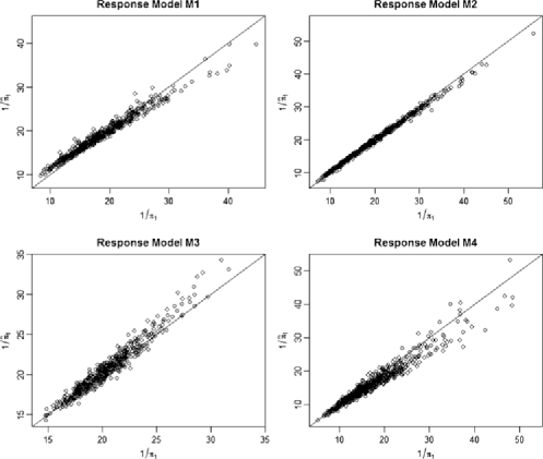
Figure 1: Plots of the fitted values on the true value of the inverse response probability under models (M1)–(M4).

5.2 Simulation two

In this simulation study, we consider only model (M5) Linear Nonignorable Measurement error. In order to test the sensitivity of model misspecification of equal coefficients for two-phase response mechanisms, we perform simulation studies by using the following response mechanisms:

$$\pi_{1i}=\frac{\exp(\phi_{0}+\phi_{1}x_{1i}+\phi_{2}z_{i})}{1+\exp(\phi_{0}+\phi_{1}x_{1i}+\phi_{2}z_{i})},\qquad\pi_{2i}=\frac{\exp(\phi^{*}_{0}+\phi_{1}x_{1i}+\phi^{*}_{2}z_{i})}{1+\exp(\phi^{*}_{0}+\phi_{1}x_{1i}+\phi^{*}_{2}z_{i})},$$

where $(\phi_{0},\phi_{1},\phi_{2},\phi^{*}_{0},\phi^{*}_{2})=(-3.4,0.3,0.1+d,0.5,0.1)$. Specifically, we consider the following three cases: [(C3)]

Small Difference: $d=0.01$.

Medium Difference: $d=0.05$.

Big Difference: $d=0.1$. Other setups of simulation two are the same as that for simulation one. The results are presented in Table 3. According to Table 3, the biases for all the proposed estimators increase when the discrepancy parameter $d$ increases, but the biases are still very modest. The variance estimators show very small relative biases, which confirms the stability of the variance estimators. Other patterns of the results are similar to that for simulation one.

Table 3: Simulation results of the point estimators and variance estimators under model (M5) for simulation two

Model	Parameter	Method	Bias	SE	RMSE	RB
(C1)	$\theta_{1}$	Naive	$0.1426$	0.0837	0.1653	N/A
		PS	$-0.0199$	0.1731	0.1742	$0.0228$
		REG	$-0.0213$	0.1627	0.1641	$0.0279$
		OPT	$-0.0194$	0.1607	0.1618	$0.0281$
	$\theta_{2}$	Naive	$0.1852$	0.0929	0.2071	N/A
		PS	$0.0066$	0.1607	0.1608	$0.0080$
		REG	$0.0059$	0.1627	0.1628	$0.0026$
		OPT1	$0.0076$	0.1605	0.1607	$-0.0099$
		OPT2	$0.0064$	0.1486	0.1487	$-0.0071$
(C2)	$\theta_{1}$	Naive	$0.2043$	0.0802	0.2194	N/A
		PS	$0.0384$	0.1726	0.1768	$-0.0213$
		REG	$0.0239$	0.1609	0.1626	$0.0157$
		OPT	$0.0295$	0.1601	0.1628	$-0.0048$
	$\theta_{2}$	Naive	$0.2457$	0.0892	0.2614	N/A
		PS	$0.0610$	0.1597	0.1709	$-0.0182$
		REG	$0.0599$	0.1611	0.1718	$-0.0168$
		OPT1	$0.0628$	0.1602	0.1720	$-0.0427$
		OPT2	$0.0529$	0.1480	0.1572	$-0.0273$
(C3)	$\theta_{1}$	Naive	$0.2992$	0.0797	0.3096	N/A
		PS	$0.1093$	0.1678	0.2002	$-0.0221$
		REG	$0.0763$	0.1605	0.1777	$-0.0131$
		OPT	$0.0887$	0.1597	0.1826	$-0.0446$
	$\theta_{2}$	Naive	$0.3533$	0.0931	0.3654	N/A
		PS	$0.1357$	0.1566	0.2072	$-0.0078$
		REG	$0.1353$	0.1587	0.2085	$-0.0115$
		OPT1	$0.1374$	0.1573	0.2089	$-0.0355$
		OPT2	$0.1158$	0.1498	0.1893	$-0.0644$

6 Empirical study

The proposed two-phase propensity score estimator is applied to the data obtained from the 2012 Iowa Caucus Survey (ICS). The Iowa political party caucuses are a significant component of the presidential candidate selection process. In 2011, two caucus polls were conducted to be implemented prior to the January 2012 Iowa Republican Caucus. In the first poll, approximately 1200 registered Republicans and Independents (no party) were interviewed in November 2011. The second poll was a follow-up conducted in December 2011 with the November 2011 respondents to identify changes in their voting preferences.

The sampling frame for the November 2011 poll was constructed from the Iowa voter registry provided by the Iowa Secretary of State. The telephone numbers on the list were reported by voters at the time of their registration and therefore included both landlines and cell phone numbers. A stratified systematic sampling design was used to select the initial sample. Five variables were used to create strata or sorting variables to ensure spread across the range of variation in age, voter activity, geography, gender and party affiliation. One indicator variable was created to differentiate voters 35 years or above from younger voters, and a second indicator variable defined whether a voter had attended one or more of the previous five primaries. Three additional variables used in designing the sample were congressional district, registered party and gender.

Strata were defined by party affiliation, congressional district, the age indicator and the prior primary attendance indicator. Within parties, sample size allocation incorporated an oversampling of primary attendees to maximize the chances of reaching likely caucus attendees. Sample allocation across the remaining strata was defined in proportion to the number of voters in each stratum. The stratified design was implemented using a systematic probability proportional to size selection scheme. The size measure was based on the relative proportion of voters in each stratum. For each party list, the systematic selection scheme was applied to a list of voters sorted by congressional district, age indicator, previous primary attendance indicator and gender.

A sample of 9000 voters was selected for the November 2011 poll, consisting of 6000 Republicans and 3000 Independents. Telephone numbers were unavailable for 836 of the sampled voters. The remaining 8164 sample households were contacted. Excluding 190 noneligible numbers, 1256 registered voters were finally interviewed from the November poll, which resulted in a 15.8 percent response rate. The November survey of registered Republicans and Independents contained questions related to anticipated caucus attendance, candidates of choice and opinions on candidate characteristics, as well as demographic and background items. In the December 2011 poll, 1256 respondents from the November poll were contacted again for a follow-up survey and 940 interviews were completed, leading to a 74.9 percent response rate. Figure 2 summarizes the two-phase sampling structure of the 2012 Iowa Caucus Survey.

Figure 2: Sample structure of 2012 Iowa Caucus Survey.

To apply our proposed method to the ICS data, let $Y$ be the reported value of the “First Choice” candidate. After preliminary analysis, we decided to use $X=(\mathrm{Party},\mathrm{Age})$ as the auxiliary variable in the propensity model. The auxiliary variable has a known total at the population level and is also related to the survey participation rate. The population size is $N={}$1,315,981. Denote $DY_{1}$ and $DY_{2}$ as the dummy variables of “First Choice” based on the first sample $A_{1}$ and the second sample $A_{2}$, and let $DX$ be the dummy variable based on $X$. Then the parameters of interest are

$$\theta_{1}=\frac{\sum_{i\in U}Z_{i}DY_{1i}}{\sum_{i\in U}Z_{i}}$$

and

$$\theta_{2}=\frac{\sum_{i\in U}Z_{i}DY_{2i}}{\sum_{i\in U}Z_{i}},$$

where $Z_{i}$ is the indicator of “Caucus Attendance” for unit $i$. That is, $Z_{i}=1$ if “Caucus Attendance${}={}$Definitely attend” or “Caucus Attendance${}={}$Likely to attend.” The outcome of the Iowa Caucus on January 3, 2012 is

$$\theta_{0}=(24.5\%,10.3\%,21.4\%,43.7\%)$$ (22)

for “First Choice” candidate: Romney, Perry, Paul, Others. Note that our parameters $\theta_{1}$ and $\theta_{2}$ are not necessarily equal to $\theta_{0}$, although they may be close for certain candidates.

The propensity model used for the proposed estimator is

$$\pi_{1i}(\phi)=\frac{\exp(\phi_{0}+\phi^{\prime}_{1}DX_{i}+\phi^{\prime}_{2}DY_{1i})}{1+\exp(\phi_{0}+\phi^{\prime}_{1}DX_{i}+\phi^{\prime}_{2}DY_{1i})}$$ (23)

and

$$\pi_{2i}\bigl{(}\phi^{*}\bigr{)}=\frac{\exp(\phi^{*}_{0}+\phi^{\prime}_{1}DX_{i}+\phi^{\prime}_{2}DY_{2i})}{1+\exp(\phi^{*}_{0}+\phi^{\prime}_{1}DX_{i}+\phi^{\prime}_{2}DY_{2i})},$$ (24)

where $DX_{i}=(DX_{1i},DX_{2i})^{\prime}$, $DY_{1i}=(DY_{11i},DY_{12i},DY_{13i},DY_{14i},DY_{15i})^{\prime}$ and $DY_{2i}=(DY_{21i},DY_{22i},DY_{23i},DY_{24i},DY_{25i})^{\prime}$. Using the proposed methods in Section 3, we obtain parameter estimates for the selection model. The estimated parameters are given in Table 4. Table 4 shows that variables $DX_{1}$, $DX_{2}$ and $DY_{11}$ have significant effects on the selection mechanisms, which supports our model for nonignorable sample selection.

Table 4: Estimated coefficients in the propensity model

Coefficient	Age	Party	Romney	Perry	Paul	Others
Est	0.588	0.782	0.991	0.454	0.866	1.307
SE	0.266	0.251	0.454	0.663	0.841	0.985
$t$-value	2.211	3.116	2.183	0.685	1.030	1.327

We consider three estimators for estimating $\theta_{t}$ for $t=1,2$: (i) the naive estimator (Naive) based on the respondents, computed by $\hat{\theta}_{tN}=\sum_{i\in A_{t}}Z_{i}DY_{ti}/\break\grave{}(\sum_{i\in A_{t}}Z_{i})$; (ii) the ignorable-response estimator (Ignorable), computed by $\hat{\theta}_{tIE}=\sum_{i\in A_{t}}\omega_{ti}Z_{i}DY_{ti}/(\sum_{i\in A_{t}}\omega_{ti}Z_{i})$, where $\omega_{ti}$ is the propensity score obtained by assuming the ignorable adjustment weight which is obtained by setting $\phi_{2}=0$ in the sample selection model; and (iii) the proposed propensity score estimator using nonignorable sample selection models in (23) and (24). The proposed propensity score estimators are computed by (5) and (6).

Table 5: Estimated parameters (s.e.) for 2012 Iowa Caucus Survey results

Survey	Method	Romney	Perry	Paul	Others
November	Naive	0.340	0.108	0.130	0.422
	Ignorable	0.316	0.103	0.146	0.435
	Proposed	0.303	0.106	0.093	0.499
		(0.062)	(0.039)	(0.107)	(0.046)
December	Naive	0.281	0.140	0.131	0.448
	Ignorable	0.270	0.144	0.148	0.437
	Proposed	0.244	0.134	0.112	0.509
		(0.043)	(0.026)	(0.046)	(0.036)

[]Standard errors are in parentheses.

The results for point estimation are given in Table 5. The proposed estimates are closer to the Iowa Caucus results in (22) than the other estimates for Romney and Perry. Furthermore, the proposed method enables us to compute the estimated standard errors of the point estimates using the theory discussed in Section 3. The estimated standard errors in the December 2011 survey estimates are smaller than those in the November 2011 survey estimates, which is consistent with our findings in Section 5. However, the estimates for Paul and Others are further away from the reported true values compared to other estimators, which are not that encouraging. It may be due to the uncontrolled time effect.

7 Concluding remarks

Estimators from self-selected samples can suffer from selection bias. Propensity score weighting using demographic variables can reduce selection bias, but the bias may remain important if survey participation depends on the study variable itself. We make assumptions about the selection mechanism that explicitly include the study variable in the selection model. To estimate the model parameters, we propose obtaining a second survey from the original self-selected sample. If the second survey has questions similar to the first one, we may assume that the regression coefficients for the explanatory variables in the propensity model are the same as for the original sample. The propensity model is then identified and the model parameters can be estimated using a generalized method of moments. The proposed method also permits estimation of the standard errors of the estimated parameters.

As mentioned in Remark 3.2, our proposed approach is equivalent to the measurement error model approach of McCaffrey, Lockwood and Setodji (2013) for propensity score weighting. Also, two limited simulation studies in Section 5 suggest that the proposed method is robust against the failure of the assumed response models and individual-level heterogeneity in the propensity to respond that persists over time. The proposed estimators have modest biases even when the equality of coefficients for the two response mechanisms violate in a certain range.

The proposed method provides a useful tool for analyzing voluntary samples as well as nonignorable nonresponse problems for survey data and, in particular, web-based panel surveys. In a panel survey, the same sample can be contacted several times and the proposed two-phase estimation approach can be extended to multiphase estimation. This is a topic of future study.

Acknowldegments

We thank two anonymous referees and the Associate Editor for their constructive comments which have helped to improve the quality of the paper. The data collection process was prepared and conducted by staff from the Center for Survey Statistics and Methodology (CSSM) and Survey and Behavioral Research Services (SBRS) at Iowa State University.

[id=suppA] Supplement Derivations Supplement Derivations for Sections 3 and 4 [doi]10.1214/14-AOAS746SUPPA .pdf aoas746_suppA.pdf Details of derivations for variances and variance estimators in Sections 3 and 4.

[id=suppB] Supplement Justifications Supplement Justifications for Remark 3.2 [doi]10.1214/14-AOAS746SUPPB .pdf aoas746_suppB.pdf Details of justifications for Remark 3.2.

References

- Baker et al. (2013) {barticle}[auto:STB—2014/06/18—12:29:53] \bauthor\bsnmBaker, \bfnmR.\binitsR., \bauthor\bsnmBrick, \bfnmJ. M.\binitsJ. M., \bauthor\bsnmBates, \bfnmN. A.\binitsN. A., \bauthor\bsnmBattaglia, \bfnmM.\binitsM., \bauthor\bsnmCouper, \bfnmM. P.\binitsM. P., \bauthor\bsnmDever, \bfnmJ. A.\binitsJ. A., \bauthor\bsnmGile, \bfnmK. J.\binitsK. J. and \bauthor\bsnmTourangeau, \bfnmR.\binitsR. (\byear2013). \btitleSummary report of the AAPOR task force on nonprobability sampling. \bjournalJ. Surv. Stat. Methodol. \bvolume1 \bpages90–143. \bptokimsref\endbibitem
- Chen and Kim (2014a) {bmisc}[auto:STB—2014/06/18—12:29:53] \bauthor\bsnmChen, \bfnmS.\binitsS. and \bauthor\bsnmKim, \bfnmJ. K.\binitsJ. K. (\byear2014a). \bhowpublishedSupplement to “Two-phase sampling experiment for propensity score estimation in self-selected samples.” DOI:\doiurl10.1214/14-AOAS746SUPPA. \bptokimsref\endbibitem
- Chen and Kim (2014b) {bmisc}[auto:STB—2014/06/18—12:29:53] \bauthor\bsnmChen, \bfnmS.\binitsS. and \bauthor\bsnmKim, \bfnmJ. K.\binitsJ. K. (\byear2014b). \bhowpublishedSupplement to “Two-phase sampling experiment for propensity score estimation in self-selected samples.” DOI:\doiurl10.1214/14-AOAS746SUPPB. \bptokimsref\endbibitem
- Deville and Särndal (1992) {barticle}[mr] \bauthor\bsnmDeville, \bfnmJean-Claude\binitsJ.-C. and \bauthor\bsnmSärndal, \bfnmCarl-Erik\binitsC.-E. (\byear1992). \btitleCalibration estimators in survey sampling. \bjournalJ. Amer. Statist. Assoc. \bvolume87 \bpages376–382. \bidissn=0162-1459, mr=1173804 \bptokimsref\endbibitem
- Duncan and Stasny (2001) {barticle}[auto:STB—2014/06/18—12:29:53] \bauthor\bsnmDuncan, \bfnmK. B.\binitsK. B. and \bauthor\bsnmStasny, \bfnmE. A.\binitsE. A. (\byear2001). \btitleUsing propensity scores to control coverages bias in telephone surveys. \bjournalSurv. Methodol. \bvolume27 \bpages121–130. \bptokimsref\endbibitem
- Durrant and Skinner (2006) {barticle}[auto:STB—2014/06/18—12:29:53] \bauthor\bsnmDurrant, \bfnmG. B.\binitsG. B. and \bauthor\bsnmSkinner, \bfnmC.\binitsC. (\byear2006). \btitleUsing missing data methods to correct for measurement error in a distribution function. \bjournalSurv. Methodol. \bvolume32 \bpages25–36. \bptokimsref\endbibitem
- Folsom and Singh (2000) {binproceedings}[auto:STB—2014/06/18—12:29:53] \bauthor\bsnmFolsom, \bfnmR. E.\binitsR. E. and \bauthor\bsnmSingh, \bfnmA. C.\binitsA. C. (\byear2000). \btitleThe generalized exponential model for sampling weight calibration for extreme values, nonresponse, and poststratification. In \bbooktitleProceedings of the Section on Survey Research Methods \bpages598–603. \bpublisherAmer. Statist. Assoc., \blocationAlexandria, VA. \bptokimsref\endbibitem
- Fuller (2002) {barticle}[auto:STB—2014/06/18—12:29:53] \bauthor\bsnmFuller, \bfnmW. A.\binitsW. A. (\byear2002). \btitleRegression estimation for sample surveys. \bjournalSurv. Methodol. \bvolume28 \bpages5–23. \bptokimsref\endbibitem
- Fuller, Loughin and Baker (1994) {barticle}[auto:STB—2014/06/18—12:29:53] \bauthor\bsnmFuller, \bfnmW. A.\binitsW. A., \bauthor\bsnmLoughin, \bfnmM. M.\binitsM. M. and \bauthor\bsnmBaker, \bfnmH. D.\binitsH. D. (\byear1994). \btitleRegression weighting for the 1987–1988 national food consumption survey. \bjournalSurv. Methodol. \bvolume20 \bpages75–85. \bptokimsref\endbibitem
- Groves, Eleanor and Amy (2000) {barticle}[auto:STB—2014/06/18—12:29:53] \bauthor\bsnmGroves, \bfnmR.\binitsR., \bauthor\bsnmEleanor, \bfnmS.\binitsS. and \bauthor\bsnmAmy, \bfnmC.\binitsC. (\byear2000). \btitleLeverage-salience theory of survey participation: Descriptiona and illustration. \bjournalPublic. Opin. Quart. \bvolume64 \bpages299–308. \bptokimsref\endbibitem
- Groves, Presser and Dipko (2004) {barticle}[auto:STB—2014/06/18—12:29:53] \bauthor\bsnmGroves, \bfnmR.\binitsR., \bauthor\bsnmPresser, \bfnmS.\binitsS. and \bauthor\bsnmDipko, \bfnmS.\binitsS. (\byear2004). \btitleThe role of topic interest in survey participation decisions. \bjournalPublic. Opin. Quart. \bvolume68 \bpages2–31. \bptokimsref\endbibitem
- Hidiroglou and Särndal (1998) {barticle}[auto:STB—2014/06/18—12:29:53] \bauthor\bsnmHidiroglou, \bfnmM. A.\binitsM. A. and \bauthor\bsnmSärndal, \bfnmC. E.\binitsC. E. (\byear1998). \btitleUse of auxiliary information for two-phase sampling. \bjournalSurv. Methodol. \bvolume24 \bpages11–20. \bptokimsref\endbibitem
- Kim and Riddles (2012) {barticle}[auto:STB—2014/06/18—12:29:53] \bauthor\bsnmKim, \bfnmJ. K.\binitsJ. K. and \bauthor\bsnmRiddles, \bfnmM.\binitsM. (\byear2012). \btitleSome theory for propensity scoring adjustment estimator. \bjournalSurv. Methodol. \bvolume38 \bpages157–165. \bptokimsref\endbibitem
- Kim and Yu (2011) {barticle}[auto:STB—2014/06/18—12:29:53] \bauthor\bsnmKim, \bfnmJ. K.\binitsJ. K. and \bauthor\bsnmYu, \bfnmC. L.\binitsC. L. (\byear2011). \btitleReplication variance estimation under two-phase sampling. \bjournalSurv. Methodol. \bvolume37 \bpages67–74. \bptokimsref\endbibitem
- Kott (2006) {barticle}[auto:STB—2014/06/18—12:29:53] \bauthor\bsnmKott, \bfnmP. S.\binitsP. S. (\byear2006). \btitleUsing calibration weighting to adjust for nonresponse and coverage errors. \bjournalSurv. Methodol. \bvolume32 \bpages133–142. \bptokimsref\endbibitem
- Kott and Chang (2010) {barticle}[mr] \bauthor\bsnmKott, \bfnmPhillip S.\binitsP. S. and \bauthor\bsnmChang, \bfnmTed\binitsT. (\byear2010). \btitleUsing calibration weighting to adjust for nonignorable unit nonresponse. \bjournalJ. Amer. Statist. Assoc. \bvolume105 \bpages1265–1275. \biddoi=10.1198/jasa.2010.tm09016, issn=0162-1459, mr=2752620 \bptokimsref\endbibitem
- Lee (2006) {barticle}[auto:STB—2014/06/18—12:29:53] \bauthor\bsnmLee, \bfnmS.\binitsS. (\byear2006). \btitlePropensity score adjustment as a weighting scheme for volunteer panel web surveys. \bjournalJ. Off. Stat. \bvolume22 \bpages329–349. \bptokimsref\endbibitem
- Lee and Valliant (2009) {barticle}[mr] \bauthor\bsnmLee, \bfnmSunghee\binitsS. and \bauthor\bsnmValliant, \bfnmRichard\binitsR. (\byear2009). \btitleEstimation for volunteer panel web surveys using propensity score adjustment and calibration adjustment. \bjournalSociol. Methods Res. \bvolume37 \bpages319–343. \biddoi=10.1177/0049124108329643, issn=0049-1241, mr=2649463 \bptokimsref\endbibitem
- Legg and Fuller (2009) {bincollection}[auto] \bauthor\bsnmLegg, \bfnmJason C.\binitsJ. C. and \bauthor\bsnmFuller, \bfnmWayne A.\binitsW. A. (\byear2009). \btitleTwo-phase sampling. In \bbooktitleSample Surveys: Theory, Methods and Inference (\beditor\bfnmD.\binitsD. \bsnmPfeffermann and \beditor\bfnmC. R.\binitsC. R. \bsnmRao, eds.). \bpublisherWiley, \blocationNew York. \bptokimsref\endbibitem
- Lundstöm and Särndal (1999) {barticle}[auto:STB—2014/06/18—12:29:53] \bauthor\bsnmLundstöm, \bfnmS.\binitsS. and \bauthor\bsnmSärndal, \bfnmC. E.\binitsC. E. (\byear1999). \btitleCalibration as a standard method for treatment of nonresponse. \bjournalJ. Off. Stat. \bvolume15 \bpages305–327. \bptokimsref\endbibitem
- McCaffrey, Lockwood and Setodji (2013) {barticle}[mr] \bauthor\bsnmMcCaffrey, \bfnmDaniel F.\binitsD. F., \bauthor\bsnmLockwood, \bfnmJ. R.\binitsJ. R. and \bauthor\bsnmSetodji, \bfnmClaude M.\binitsC. M. (\byear2013). \btitleInverse probability weighting with error-prone covariates. \bjournalBiometrika \bvolume100 \bpages671–680. \biddoi=10.1093/biomet/ast022, issn=0006-3444, mr=3094444 \bptokimsref\endbibitem
- Rao (1994) {barticle}[auto:STB—2014/06/18—12:29:53] \bauthor\bsnmRao, \bfnmJ. N. K.\binitsJ. N. K. (\byear1994). \btitleEstimation of totals and distributing functions using auxiliary information at the estimation stage. \bjournalJ. Off. Stat. \bvolume10 \bpages153–165. \bptokimsref\endbibitem
- Rosenbaum (1987) {barticle}[auto:STB—2014/06/18—12:29:53] \bauthor\bsnmRosenbaum, \bfnmP. R.\binitsP. R. (\byear1987). \btitleModel-based direct adjustment. \bjournalJ. Amer. Statist. Assoc. \bvolume82 \bpages387–394. \bptokimsref\endbibitem
- Rosenbaum and Rubin (1983) {barticle}[mr] \bauthor\bsnmRosenbaum, \bfnmPaul R.\binitsP. R. and \bauthor\bsnmRubin, \bfnmDonald B.\binitsD. B. (\byear1983). \btitleThe central role of the propensity score in observational studies for causal effects. \bjournalBiometrika \bvolume70 \bpages41–55. \biddoi=10.1093/biomet/70.1.41, issn=0006-3444, mr=0742974 \bptokimsref\endbibitem
- Rubin (1976) {barticle}[mr] \bauthor\bsnmRubin, \bfnmDonald B.\binitsD. B. (\byear1976). \btitleInference and missing data. \bjournalBiometrika \bvolume63 \bpages581–592. \bidissn=0006-3444, mr=0455196 \bptokimsref\endbibitem
- Valliant and Dever (2011) {barticle}[mr] \bauthor\bsnmValliant, \bfnmRichard\binitsR. and \bauthor\bsnmDever, \bfnmJill A.\binitsJ. A. (\byear2011). \btitleEstimating propensity adjustments for volunteer web surveys. \bjournalSociol. Methods Res. \bvolume40 \bpages105–137. \biddoi=10.1177/0049124110392533, issn=0049-1241, mr=2758301 \bptokimsref\endbibitem