Identifying a superfluid Reynolds number via dynamical similarity

Abstract

The Reynolds number provides a characterization of the transition to turbulent flow, with wide application in classical fluid dynamics. Identifying such a parameter in superfluid systems is challenging due to their fundamentally inviscid nature. Performing a systematic study of superfluid cylinder wakes in two dimensions, we observe dynamical similarity of the frequency of vortex shedding by a cylindrical obstacle. The universality of the turbulent wake dynamics is revealed by expressing shedding frequencies in terms of an appropriately defined superfluid Reynolds number, ${\rm Re}_{s}$, that accounts for the breakdown of superfluid flow through quantum vortex shedding. For large obstacles, the dimensionless shedding frequency exhibits a universal form that is well-fitted by a classical empirical relation. In this regime the transition to turbulence occurs at $\mathrm{Re}_{s}\approx 0.7$, irrespective of obstacle width.

Turbulence in classical fluid flows emerges from the competition between viscous and inertial forces. For a flow with characteristic length scale $L$, velocity $u$, and kinematic viscosity $\nu$, the dimensionless Reynolds number $\mathrm{Re}=uL/\nu$ characterizes the onset and degree of turbulent motion. A naive evaluation of the Reynolds number for an ideal superfluid is thwarted by the absence of kinematic viscosity, suggesting that the classical Reynolds number of a superfluid is formally undefined Barenghi (2008); Sasaki et al. (2010); Stagg et al. (2014). However, for sufficiently rapid flows, perfect inviscid flow breaks down and an effective viscosity emerges dynamically via the nucleation of quantized vortices Frisch et al. (1992). As noted by Onsager Onsager (1953), the quantum of circulation of a superfluid vortex, given by the ratio of Planck’s constant to the atomic mass, $h/m$, has the same dimension as $\nu$. This suggests making the replacement $\nu\rightarrow h/m$, giving a superfluid Reynolds number $\mathrm{Re}_{s}\sim uLm/h$ Volovik (2003); L’vov et al. (2014). This approach is supported by evidence that this quantity accounts for the degree of superfluid turbulence when $\mathrm{Re}_{s}\gg 1$ Nore et al. (1997); Abid et al. (1998); Nore et al. (2000); Hänninen et al. (2007), but has yet to be tested by a detailed study of the transition to turbulence.

The wake of a cylinder embedded in a uniform flow is a paradigmatic example of the transition to turbulence Williamson (1996), and has been partially explored in the context of quantum turbulence in atomic Bose-Einstein condensates (BECs) Frisch et al. (1992); Winiecki et al. (1999, 2000); Sasaki et al. (2010); Stagg et al. (2014). The classical fluid wakes are dynamically similar: for cylinder diameter $D$ and free-stream velocity $u$ their physical characteristics are parametrized entirely by $\mathrm{Re}=uD/\nu$. Above a critical Reynolds number, vortices of alternating circulation shed from the obstacle with characteristic frequency $f$. As a consequence of dynamical similarity, the associated dimensionless Strouhal number $\mathrm{St}\equiv fD/u$ takes a universal form when plotted against the Reynolds number. In the context of a superfluid, the Strouhal number is a measurable quantity that can be used to define the superfluid Reynolds number as a dimensionless combination of flow parameters that reveals dynamical similarity.

In this Letter we numerically study the Strouhal–Reynolds relation across the transition to turbulence in quantum cylinder wakes of the two-dimensional Gross-Piteaveskii equation. We develop a numerical approach to gain access to quasi-steady-state properties of the wake for a wide range of system parameters, and to accurately determine the Strouhal number $\mathrm{St}$. We find that plotting $\mathrm{St}$ against a superfluid Reynolds number defined as

$$\mathrm{Re}_{s}\equiv\frac{(u-u_{c})D}{\kappa},$$ (1)

where $u_{c}$ is the superfluid critical velocity and $\kappa\equiv\hbar/m$ , reveals dynamical similarity in the quantum cylinder wake: for obstacles larger than a few healing lengths the wakes exhibit a universal $\mathrm{St}$–$\mathrm{Re}_{s}$ relation similar to the classical form. Furthermore, for these obstacles $\mathrm{Re}_{s}$ characterises the transition to quantum turbulence, with irregularities spontaneously developing in the wake when $\mathrm{Re}_{s}\approx 0.7$, irrespective of cylinder size.

We consider a Gaussian stirring potential moving at a steady velocity $\mathbf{u}$ through a superfluid that is otherwise uniform in the $xy$-plane and subject to tight harmonic confinement in the $z$-direction. In the obstacle reference frame with coordinate $\mathbf{r}=\mathbf{r}_{L}+\mathbf{u}t$, the time evolution of the lab-frame wavefunction $\psi(\mathbf{r},t)=\psi_{L}(\mathbf{r}_{L},t)$ is governed by the Gross-Pitaevskii equation (GPE);

$$i\hbar\frac{\partial\psi(\mathbf{r},t)}{\partial t}=(\mathcal{L}-\mathbf{u}\cdot\mathbf{p}-\mu)\psi(\mathbf{r},t),$$ (2)

where $\mu$ is the chemical potential, $\mathbf{p}=-i\hbar\nabla$, and

$$\mathcal{L}\equiv\left[-\frac{\hbar^{2}\nabla^{2}}{2m}+V_{s}(\mathbf{r})+g_{\rm{2}}|\psi(\mathbf{r},t)|^{2}\right].$$ (3)

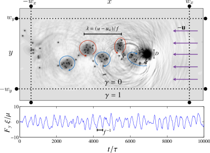
Figure 1: (color online) (Top) A quantum cylinder wake in the quasi-steady state. Same-sign vortices aggregate into clusters to form a semi-classical vortex street. Vortices within the fringe region $|x|>w_{x}$ are unwound in pairs by imprinting opposite-signed vortices on top of them, thus recycling the flow to the uniformly translating state as indicated at the right of the domain. (Bottom) Time series data of the transverse force on the obstacle. The force exhibits a well-defined frequency, which determines the Strouhal number for the flow.

Here, $g_{2}=\sqrt{8\pi}\hbar^{2}a_{s}/ml_{z}$, where $m$ is the atomic mass, $a_{s}$ is the $s$-wave scattering length, and $l_{z}=\sqrt{\hbar/m\omega_{z}}$ is the harmonic oscillator length in the $z$-direction. The trapping in the $z$-direction is assumed strong enough to suppress excitations along this direction . The stirring potential is of the form $V_{s}(\mathbf{r})=V_{0}\exp\{-[(x-x_{0})^{2}-y^{2}]/\sigma^{2}\}$, giving an effective cylinder width, $D=2a=2\sigma[\log(V_{0}/\mu)]^{1/2}$, defined by the zero-region of the density in the Thomas-Fermi approximation. In contrast to previous studies Sasaki et al. (2010); Stagg et al. (2014) employing strong potentials ($V_{0}\sim 100\mu$) to approximate a hard-walled obstacle, we use soft-walled obstacles (with $V_{0}=e\mu$, such that $D=2\sigma$): these obstacles exhibit a well-defined vanishing-density region, but have a much lower critical velocity than hard-wall obstacles Winiecki et al. (1999). A low critical velocity makes the transition to turbulence — which must occur between the critical velocity and the supersonic regime — more gradual, aiding our numerical characterization. We find that $D$ gives a good indication of the effective cylinder width for all obstacles we consider, with vortices unpinning from the obstacle at $y\approx\pm a$ (see Fig. 1).

A key innovation facilitating our study of quasi-steady-state quantum cylinder wakes is a numerical method to maintain approximately steady inflow-outflow boundary conditions in the presence of quantum vortices. This method enables us to evolve cylinder wakes for extremely long times in a smaller spatial domain, making our numerical experiment computationally feasible. In essence, we extend the sponge or fringe method Spalart (1989); Colonius (2004); Mani (2012); Nordström et al. (1999), which implements steady inflow/outflow boundary conditions by “recycling” flow in a periodic domain, to deal with quantum vortices. The spatial region of the numerical simulation is divided into a “computational domain” of interest and a “fringe domain”. Inside the fringe domain, we use a damped GPE Tsubota et al. (2002); Blakie et al. (2008) to rapidly drive the wavefunction to the lab-frame ground state with chemical potential $\mu$; a uniform state, free from excitations and moving at velocity $-\mathbf{u}$ relative to the obstacle, is thus produced at the outer boundary of the fringe regions. The modified equation of motion is thus

$$i\hbar\frac{\partial\psi(\mathbf{r},t)}{\partial t}=(\mathcal{L}-\mathbf{u}\cdot\mathbf{p}-\mu)\psi(\mathbf{r},t)-i\gamma(\mathbf{r})(\mathcal{L}_{f}-\mu)\psi(\mathbf{r},t),$$ (4)

where the free GPE evolution operator $\mathcal{L}_{f}\equiv\mathcal{L}-V_{s}(\mathbf{r})$. At the computational/fringe boundary $(x,y)=(\pm w_{x},\pm w_{y})$, $\gamma$ must ramp smoothly from zero to a large value to prevent reflections, with hyperbolic tangent functions a common choice Colonius (2004). We set $\gamma(\mathbf{r})=\max[\gamma(x),\gamma(y)],$ where $\gamma(x)=\gamma_{0}\{2+\tanh[(x-w_{x})/d]-\tanh[(x+w_{x})/d]\}/2$ and similarly for $\gamma(y)$.

Quantum vortices, as topological excitations, decay only at the fluid boundary or by annihilation with opposite-sign vortices. While damping drives opposite-signed vortices together at a rate proportional to $\gamma$ Törnkvist and Schröder (1997), relying on this mechanism to avoid vortices being “recycled” around the simulation domain requires a prohibitively large fringe domain when the wake exhibits clustering of like-sign vortices, a key feature of the transition to turbulence. Instead, we unwind vortex-antivortex pairs within the fringe domain by phase imprinting an antivortex-vortex pair on top them, using the rapidly converging expression for the phase of a vortex dipole in a periodic domain derived in Ref. Billam et al. (2014). When vortices of only one sign exist within the fringe region, the same method is used to “reset” vortices back near the start of the fringe ($x=-w_{x}$) to avoid them being recycled. The high damping in the fringe domain rapidly absorbs the energy added by this imprinting.

Working in units of the the healing length $\xi=\hbar/\sqrt{m\mu}$, the speed of sound $c=\sqrt{\mu/m}$ and time unit $\tau=\hbar/\mu$, we discretize a spatial domain of $L_{x}=512\xi$ by $L_{y}=256\xi$ on a grid of $M_{x}=1024$ by $M_{y}=512$ points. The obstacle is positioned at $x_{0}=100\xi$, and for the fringe domain we set $w_{x}=220\xi$, $w_{y}=100\xi$, $d=7\xi$ and $\gamma_{0}=1$ .

A typical result from this setup is shown in Fig. 1. We integrate Eq. (4) pseudospectrally, for sufficient time to accurately resolve the cluster shedding frequency $f$ (see Fig. 1, bottom panel). A small amount of initial noise is added to break the symmetry. Analyzing obstacles in the range $4\leq D/\xi\leq 24$ requires integration times $5000\leq T/\tau\leq 12000$, representing a significant computational challenge. To determine the Strouhal number $\mathrm{St}=fD/u$ we calculate the transverse force on the obstacle from the Ehrenfest relation, $F_{y}=\int d^{2}\mathbf{r}\;\psi^{*}(\partial_{y}V_{s})\psi$, with $f$ being defined by the dominant mode in the frequency power spectrum of $F_{y}$.

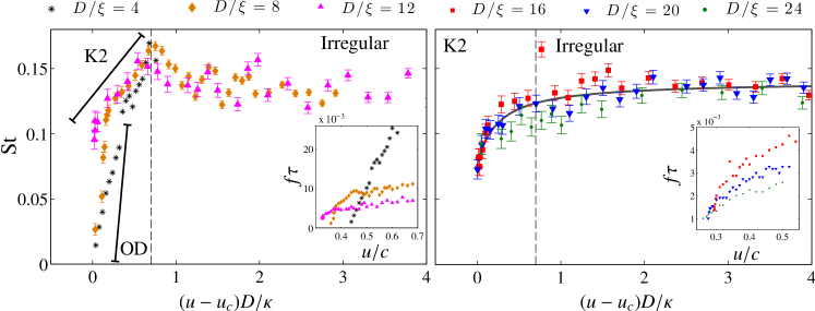
Figure 2: (color online) Strouhal number plotted as a function of the superfluid Reynolds number for obstacles of different diameters $D$. The dashed lines indicate the transition between regular and irregular wakes (see text). Solid lines in the left panel indicate regions of oblique dipole (OD) and charge-2 von Kármán (K2) shedding. The solid gray line shows the best-fit curve $\mathrm{St}=0.1402[1-0.1126/(\mathrm{Re}_{s}+0.2456)]$. Error bars give an indication of the uncertainty in $\mathrm{St}$ due to the Fourier-space resolution $\Delta f=1/T$. Insets show the original shedding frequency data as a function of velocity. The data for $D/\xi=4$ is truncated as the shedding frequency becomes poorly defined at higher velocities for this particular obstacle. In the Supplemental Material sup we provide movies showing condensate density and vortex-cluster dynamics in each shedding regime.

Our main results are shown in Fig. 2, where the Strouhal number $\mathrm{St}$ is plotted against the superfluid Reynolds number $\mathrm{Re}_{s}=(u-u_{c})D/\kappa$ for a range of obstacle diameters $D$ [insets show shedding frequency $f$ against velocity $u$]. In the Supplemental Material sup we provide movies showing condensate density and vortex-cluster dynamics for representative sets of parameters. The obstacles are broadly classified as quantum ($\sigma\leq 12\xi$, left) or semi-classical ($\sigma>12\xi$, right). For quantum obstacles the vortex core size influences the shedding dynamics, and the $\mathrm{St}$-$\mathrm{Re}_{s}$ curve exhibits three distinct regimes: At low $\mathrm{Re}_{s}$, vortex dipoles are released obliquely from the obstacle (OD regime), and St rises sharply with $\mathrm{Re}_{s}$. As $\mathrm{Re}_{s}$ is increased, the gradient of the $\mathrm{St}$-$\mathrm{Re}_{s}$ curve drops sharply when a charge-2 von Kármán vortex street Sasaki et al. (2010) appears (K2 regime). The Strouhal number peaks at $\mathrm{Re}_{s}\sim 0.7,\mathrm{St}\approx 0.16$, and beyond this point the shedding becomes irregular, and the Strouhal number gradually decreases towards $\mathrm{St}\approx 0.14$. The $\mathrm{St}$-$\mathrm{Re}_{s}$ data conform to a single curve rather well when compared against the $f$ vs. $u$ data shown in the inset, apart from variation in the OD regime at low $\mathrm{Re}_{s}$. This can be attributed to the influence of vortex core structure on shedding, which is most pronounced for $D/\xi=4$. At $D/\xi=12$ the curve becomes very steep, and dipole shedding seems to disappear.

For semi-classical obstacles (right panel of Fig. 2), the $\mathrm{St}$-$\mathrm{Re}_{s}$ curve is qualitatively different. Obstacles with $D/\xi\geq 12$ appear to lack a stable OD regime , and the most steeply-rising region of the $\mathrm{St}$-$\mathrm{Re}$ curve corresponds to the K2 regime. The peak seen in the $\mathrm{St}$-$\mathrm{Re}_{s}$ curve for quantum obstacles is generally absent (with a remnant for $D/\xi=16$), and the $\mathrm{St}$-$\mathrm{Re}_{s}$ data conform to a universal curve extremely well for $\mathrm{Re}_{s}\lesssim 0.5$ and $\mathrm{Re}_{s}\gtrsim 2$, and to a lesser extent around $\mathrm{Re}_{s}=1$. This discrepancy may be an effect of using a soft-walled obstacle, for which varying $\sigma$ for fixed $V_{0}$ leads to a slight change in the density profile near the obstacle. Remarkably, the $\mathrm{St}$-$\mathrm{Re}_{s}$ curve for the semiclassical obstacles is well-fitted by the formula $\mathrm{St}=\mathrm{St}_{\infty}[1-\alpha/(\mathrm{Re}_{s}+\beta)]$  , which is similar to the classical form $\mathrm{St}=\mathrm{St}_{\infty}(1-A/\mathrm{Re})$  Roshko (1954a).

To test whether $\mathrm{Re}_{s}$ provides an accurate indicator of the transition to quantum turbulence, in Fig. 3 we show the vortex-cluster charge probability distribution, $\mathcal{P}(\kappa_{c},\mathrm{Re}_{s})$. This indicates the probability of any vortex belonging to a cluster of charge $\kappa_{c}$, as determined by the recursive cluster algorithm of Ref. Reeves et al. (2013). The transition to turbulence manifests as an abrupt spreading in $\mathcal{P}$ at $\mathrm{Re}_{s}\approx 0.7$. The distribution $\mathcal{P}$ is similar for all obstacles except the smallest ($D/\xi=4$) where high $\mathrm{Re}_{s}$ vortex turbulence is suppressed by compressible effects due to the transsonic velocities involved. Notice that the distribution is close to independent of obstacle size for larger obstacles ($D\geq 12\xi$). We find that the K2 regime persists for a significant range of $\mathrm{Re}_{s}$ even for large $D$, in contrast to Ref. Sasaki et al. (2010). We suggest the vanishing of the K2 regime at large $D$ seen in Ref. Sasaki et al. (2010) may be due to the higher critical velocity of the hard-walled obstacle. We find no regular charge-$\kappa_{c}$ von Kármán regimes (K$\kappa_{c}$ regimes) other than K2. The lack of a K1 regime, the focus of von Kármán’s original analysis of vortex streets Saffman (1995), suggests that the additional degree of freedom provided by the internal length scale of the charge-2 cluster is what enables stable vortex shedding in the K2 regime. The lack of K$\kappa_{c}$ regimes for $\kappa_{c}>2$ appears to be due to instabilities; although regimes do exist where $\mathcal{P}$ is strongly peaked around $|\kappa_{c}|>2$, such regimes do not appear to be stable.

The superfluid Reynolds number $\mathrm{Re}_{s}$ introduced in Eq. (1) serves as a good control parameter for the transition to turbulence, which occurs at $\mathrm{Re}_{s}\approx 0.7$ for all obstacle sizes investigated except $D/\xi=4$ (it is expected to fail for $D\rightarrow\xi$, where dynamical similarity is lost). The definition of $\mathrm{Re}_{s}$ in terms of $u-u_{c}$ is intuitively appealing: the subtraction of $u_{c}$ becomes unimportant in the classical limit (where $u_{c}$ vanishes) and when $\mathrm{Re}_{s}\gg 1$, consistent with previous observations Nore et al. (1997); Abid et al. (1998); Nore et al. (2000). Subtracting $u_{c}$ is consistent with previous arguments that corrections to the Reynolds number formula are necessary for quantum obstacles Hänninen et al. (2007), and reflects the fact that in a pure superfluid an effective viscosity due to quantum vortices is only “activated” once vortices are nucleated.

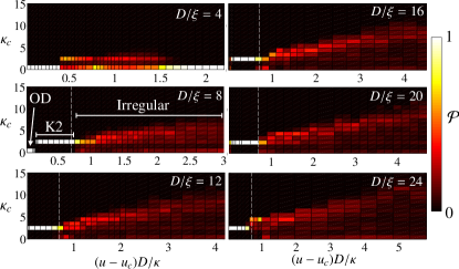
Figure 3: Cluster charge probability distribution $\mathcal{P}(\kappa_{c},\mathrm{Re}_{s})$, which shows the probability that a vortex belongs to a cluster of charge magnitude $\kappa_{c}$. Note that $\kappa_{c}=0$ corresponds to a dipole and $\kappa_{c}=1$ corresponds to a free vortex. The vertical dashed line shows the value $\mathrm{Re}_{s}=0.7$ at which the probability distribution suddenly spreads, indicating that the wake has developed irregularities. The three different shedding regimes observed are labelled for the case $D/\xi=8$.

Although $\mathrm{Re}_{s}$ takes on small values here compared to the Reynolds number of classical cylinder wakes, we note the close correspondence between the $\mathrm{St}$-$\mathrm{Re}_{s}$ curve obtained here and the classical $\mathrm{St}$-$\mathrm{Re}$ curve. The latter rises steeply when the shedding is regular, and reaches a plateau as the shedding becomes irregular Roshko (1954a). This correspondence suggests that $\mathrm{Re}_{s}\sim 0.7$ may be roughly equivalent to $\mathrm{Re}\sim 200$. The fact that the $\mathrm{St}$-$\mathrm{Re}_{s}$ curves approach a universal form for different obstacle sizes suggests that the wake structure is insensitive to considerable changes in Mach number, which occur between different obstacle widths at fixed $\mathrm{Re}_{s}$, consistent with the observation that the wake is dominated by vortex shedding even into the transonic regime Winiecki et al. (2000). The discrepancy between the asymptotic values of $\mathrm{St}$ found here and in the classical case appears to be mainly due to the use of soft-walled obstacles: we have confirmed that simulations with $V_{0}/\mu=10\exp(1)$ and $D/\xi=20$ produce a qualitatively similar $\mathrm{St}$-$\mathrm{Re}_{s}$ curve to Fig. 2 but with higher asymptote $\mathrm{St}_{\infty}\approx 0.16$. For the hard-wall obstacle of Ref. Sasaki et al. (2010) we find $\mathrm{St}\approx 0.18$ for velocities that give a vortex street, in reasonable agreement with classical observations where $\mathrm{St}_{\infty}\approx 0.2$ Ahlborn et al. (2002); Roshko (1954b). The lower Strouhal number of the soft-walled obstacle suggests that it is “bluffer” than the hard-walled one, in the sense that it produces a wider wake for a given obstacle dimension $D$ Roshko (1954b).

The K2 regime should be accessible to current BEC experiments Sasaki et al. (2010), since the wake is stable and easily identified. Accessing the high $\mathrm{Re}_{s}$ regime with fine resolution may be experimentally challenging, however, the low $\mathrm{Re}_{s}$ turbulent regime, particularly near the transition, should be accessible in current BEC experiments. In this regime the Strouhal number should be measurable, since the induced wake velocity $u_{w}\rightarrow 0$ Roshko (1954a) and thus the average streamwise cluster spacing $\lambda=(u-u_{w})/f\rightarrow u/f$ determines $\mathrm{St}=D/\lambda$.

In conclusion, we have developed a vortex-unwinding fringe method to study quasi-steady-state quantum cylinder wakes, revealing a superfluid Reynolds number $\mathrm{Re}_{s}$ that controls the transition to turbulence in the wake of an obstacle in a planar quantum fluid. The expression for $\mathrm{Re}_{s}$ resembles the classical form, modified to account for the critical velocity at which effective superfluid viscosity emerges. As the critical velocity encodes details of geometry and the microscopic nature of the superfluid, the general form of $\mathrm{Re}_{s}$ suggests that it may apply to a broad range of systems, much like the classical Reynolds number. We thus conjecture that our work may provide a useful characterisation of turbulence in any superfluid, such as liquid helium Bewley et al. (2008), polariton condensates Tosi et al. (2011), and BEC-BCS superfluidity in Fermi gases Zwierlein et al. (2005).