Minimization of Transformed $L_{1}$ Penalty: Theory, Difference of Convex Function Algorithm, and Robust Application in Compressed Sensing

Abstract

We study the minimization problem of a non-convex sparsity promoting penalty function, the transformed $l_{1}$ (TL1), and its application in compressed sensing (CS). The TL1 penalty interpolates $l_{0}$ and $l_{1}$ norms through a nonnegative parameter $a\in(0,+\infty)$, similar to $l_{p}$ with $p\in(0,1]$, and is known to satisfy unbiasedness, sparsity and Lipschitz continuity properties. We first consider the constrained minimization problem, and discuss the exact recovery of $l_{0}$ norm minimal solution based on the null space property (NSP). We then prove the stable recovery of $l_{0}$ norm minimal solution if the sensing matrix $A$ satisfies a restricted isometry property (RIP). We formulated a normalized problem to overcome the lack of scaling property of the TL1 penalty function. For a general sensing matrix $A$, we show that the support set of a local minimizer corresponds to linearly independent columns of $A$. Next, we present difference of convex algorithms for TL1 (DCATL1) in computing TL1-regularized constrained and unconstrained problems in CS. The DCATL1 algorithm involves outer and inner loops of iterations, one time matrix inversion, repeated shrinkage operations and matrix-vector multiplications. The inner loop concerns an $l_{1}$ minimization problem on which we employ the Alternating Direction Method of Multipliers (ADMM). For the unconstrained problem, we prove convergence of DCATL1 to a stationary point satisfying the first order optimality condition. In numerical experiments, we identify the optimal value $a=1$, and compare DCATL1 with other CS algorithms on two classes of sensing matrices: Gaussian random matrices and over-sampled discrete cosine transform matrices (DCT). Among existing algorithms, the iterated reweighted least squares method based on $l_{1/2}$ norm is the best in sparse recovery for Gaussian matrices, and the DCA algorithm based on $l_{1}$ minus $l_{2}$ penalty is the best for over-sampled DCT matrices. We find that for both classes of sensing matrices, the performance of DCATL1 algorithm (initiated with $l_{1}$ minimization) always ranks near the top (if not the top), and is the most robust choice insensitive to the conditioning of the sensing matrix $A$. DCATL1 is also competitive in comparison with DCA on other non-convex penalty functions commonly used in statistics with two hyperparameters.

AMS Subject Classifications: 90C26, 65K10, 90C90

1 Introduction

Compressed sensing [6, 12] has generated enormous interest and research activities in mathematics, statistics, information science and elsewhere. A basic problem is to reconstruct a sparse signal under a few linear measurements (linear constraints) far less than the dimension of the ambient space of the signal. Consider a sparse signal $x\in\Re^{N}$, an $M\times N$ sensing matrix $A$ and an observation $y\in\Re^{M}$, $M\ll N$, such that: $y=A\,x+\epsilon,$ where $\epsilon$ is an $N$-dimensional observation error. The main objective is to recover $x$ from $y$.

The direct approach is $l_{0}$ optimization in either a constrained formulation:

$$\min\limits_{x\in\Re^{N}}\|x\|_{0},\;\;s.t.\;\;\ Ax=y,$$ (1.1)

or an unconstrained $l_{0}$ regularized optimization:

$$\min\limits_{x\in\Re^{N}}\{\|y-A\,x\|_{2}^{2}+\lambda\|x\|_{0}\}$$ (1.2)

with a positive regularization parameter $\lambda$. Since minimizing $l_{0}$ norm is NP-hard [28], many viable alternatives have been sought. Greedy methods (matching pursuit [26], othogonal matching pursuits (OMP) [38], and regularized OMP (ROMP) [29]) work well if the dimension $N$ is not too large. For the unconstrained problem (1.2), the penalty decomposition method [24] replaces the term $\lambda\|x\|_{0}$ by $\rho_{k}\|x-z\|_{2}^{2}+\lambda\|z\|_{0}$, and minimizes over $(x,z)$ for a diverging sequence $\rho_{k}$. The variable $z$ allows the iterative hard thresholding procedure.

The relaxation approach is to replace $l_{0}$ norm by a continuous sparsity promoting penalty function $P(x)$. Convex relaxation uniquely selects $P(\cdot)$ as the $l_{1}$ norm. The resulting problem is known as basis pursuit (LASSO in the over-determined regime [36]). The $l_{1}$ algorithms include $l_{1}$-magic [6], Bregman and split Bregman methods [17, 44] and yall1 [41]. Theoretically, Candès, Tao and coauthors introduced the restricted isometry property (RIP) on $A$ to establish the equivalent and unique global solution to $l_{0}$ minimization and stable sparse recovery results [3, 4, 6].

There are many choices of $P(\cdot)$ for non-convex relaxation, almost all of them are known in statistics [15, 27]. One is the $l_{p}$ norm (a.k.a. bridge penalty) ($p\in(0,1)$) with known $l_{0}$ equivalence under RIP [9]. The $l_{1/2}$ norm is representative of this class of penlty functions, with the associated reweighted least squares and half-thresholding algorithms for computation [18, 40, 39]. Near the RIP regime, $l_{1/2}$ penalty tends to have higher success rate of sparse reconstruction than $l_{1}$. However, it is not as good as $l_{1}$ if the sensing matrix $A$ is far from RIP [23, 42] as we shall see later as well. In the highly non-RIP (coherent) regime, it is recently found that the difference of $l_{1}$ and $l_{2}$ norm minimization gives the best sparse recovery results [42, 23]. It is therefore of both theoretical and practical interest to find a non-convex penalty that is consistently better than $l_{1}$ and always ranks among the top in sparse recovery whether the sensing matrix satisfies RIP or not.

The $l_{p}$ penalty functions are however known to bias towards large peaks. In the statistics literature of variable selection, Fan and Li [15] advocated for classes of penalty functions with three desired properties: unbiasedness, sparsity and continuity. To help identify such a penalty function denoted by $\rho(\cdot)$, Fan and Lv [25] proposed the following condition for characterizing unbiasedness and sparsity promoting properties.

Condition 1

The penalty function $\rho(\cdot)$ satisfies:

1. $\rho(t)$ is increasing and concave in $t\in[0,\infty)$,

2. $\rho^{\prime}(t)$ is continuous with $\rho^{\prime}(0+)\in(0,\infty)$.

It follows that $\rho^{\prime}(t)$ is positive and decreasing, and $\rho^{\prime}(0+)$ is the upper bound of $\rho^{\prime}(t)$. The penalties satisfying Condition 1 and $\lim_{t\to\infty}\rho^{{}^{\prime}}(t)=0$ enjoy both unbiasedness and sparsity [25]. Though continuity does not generally hold for this class of penalty functions, a special one parameter family of Lipschitz continuous functions, the so called transformed $l_{1}$ functions [31], satisfy all three desired properties above [25].

In this paper, we show that minimizing the non-convex transformed $l_{1}$ functions (TL1) by the difference of convex (DC) function algorithm provides a robust CS solution insensitive to the conditioning of $A$. Since verifying the incoherence condition like RIP or null space property [11] on a specific matrix is NP hard, such robustness is a significant attribute of an algorithm. Let us consider TL1 function of the form [25]:

$$\rho_{a}(t)=\dfrac{(a+1)|t|}{a+|t|},\ \ \;\;\forall t\in\Re,$$ (1.3)

with parameter $a\in(0,+\infty)$, see [31, 19] for alternative forms and the $l_{0}$ approximation property [19]. Another nice property of TL1 is that the TL1 proximal operator has closed form analytical solutions for all values of parameter $a$. Fast TL1 iterative theresholding algorithms have been devised and studied for both sparse vector and low rank matrix recovery problems lately [47, 48].

The rest of the paper is organized as follows. In section 2, we study theoretical properties of TL1 penalty and TL1 regularized models in exact and stable recovery of $\ell_{0}$ minimal solutions. We show the advantage of TL1 over $\ell_{1}$ in exact recovery under linear constraint using the generalized null space property [37] and explicit examples. We analyze stable recovery for linear constraint with observation error based on a RIP condition. We overcome the lack of scaling property of TL1 by introducing a normalized TL1 regularized problem. Though the RIP condition is not sharp, our analysis is the first of such kind for stable recovery by TL1. We also prove that the local minimizers of the TL1 constrained model extract independent columns from the sensing matrix. In section 3, we present two DC algorithms for TL1 optimization (DCATL1). In section 4, we compare the performance of DCATL1 with some state-of-the-art methods using two classes of matrices: the Gaussian and the over-sampled discrete cosine transform (DCT) matrices. Numerical experiments indicate that DCATL1 is robust and consistently top ranked while maintaining high sparse recovery rates across sensing matrices of varying coherence. In section 5, we compare DCATL1 with DCA on other non-convex penalties such as PiE [30], MCP [46], and SCAD [15], and found DCATL1 to be competitive as well. Concluding remarks are in section 6.

2 Transformed $l_{1}$ (TL1) and its regularization models

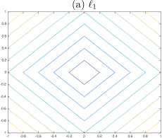
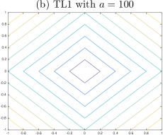
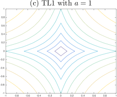
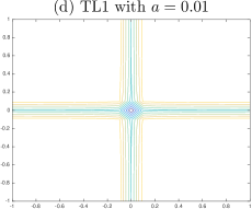
Figure 1: Level lines of TL1 with different parameters: $a=100$ (figure b), $a=1$ (figure c), $a=0.01$ (figure d). For large parameter ‘$a$’, the graph looks almost the same as $l_{1}$ (figure a). While for small value of ‘$a$’, it tends to the axis.

The TL1 penalty function $\rho_{a}(t)$ of (1.3) interpolates the $l_{0}$ and $l_{1}$ norms as

$$\lim_{a\to 0^{+}}\rho_{a}(t)=\chi_{\{t\neq 0\}}\;\;\rm{and}\;\;\lim_{a\to\infty}\rho_{a}(t)=|t|.$$

In Fig. (1), we compare level lines of $l_{1}$ and TL1 with different parameter values of ‘$a$’. With the adjustment of parameter ‘$a$’, the TL1 can approximate both $l_{1}$ and $l_{0}$ well. Let us define TL1 regularization term $P_{a}(\cdot)$ as

$$P_{a}(x)=\sum\limits_{i=1,...N}\rho_{a}(x_{i}).$$ (2.1)

In the following, we consider the constrained TL1 minimization model

$$\min\limits_{x\in\Re^{N}}f(x)=\min\limits_{x\in\Re^{N}}P_{a}(x)\;\;s.t.\;\;\ Ax=y,$$ (2.2)

and the unconstrained TL1-regularized model

$$\min\limits_{x\in\Re^{N}}f(x)=\min\limits_{x\in\Re^{N}}\frac{1}{2}\|Ax-y\|^{2}_{2}+\lambda P_{a}(x).$$ (2.3)

The following inequalities of $\rho_{a}$ will be used in the proof of TL1 theories.

Lemma 2.1

For $a\geq 0$, any $x_{i}$ and $x_{j}$ in $\Re$, the following inequalities hold:

$$\rho_{a}(|x_{i}+x_{j}|)\leq\rho_{a}(|x_{i}|+|x_{j}|)\leq\rho_{a}(|x_{i}|)+\rho_{a}(|x_{j}|)\leq 2\rho_{a}(\frac{|x_{i}|+|x_{j}|}{2}).$$ (2.4)

Proof 2.1.

Let us prove these inequalities one by one, starting from the left.

• Note that $\rho_{a}(|t|)$ is increasing in the variable $|t|$. By triangle inequality $|x_{i}+x_{j}|\leq|x_{i}|+|x_{j}|$, we have:

  $$\rho_{a}(|x_{i}+x_{j}|)\leq\rho_{a}(|x_{i}|+|x_{j}|).$$

• $$\begin{array}[c]{lll}\vspace{2mm}\rho_{a}(|x_{i}|)+\rho_{a}(|x_{j}|)&=&\dfrac{(a+1)|x_{i}|}{a+|x_{i}|}+\dfrac{(a+1)|x_{j}|}{a+|x_{j}|}\\ \vspace{2mm}&=&\dfrac{a(a+1)(|x_{i}|+|x_{j}|+2|x_{i}x_{j}|/a)}{a(a+|x_{i}|+|x_{j}|+|x_{i}x_{j}|/a)}\\ \vspace{2mm}&\geq&\dfrac{(a+1)(|x_{i}|+|x_{j}|+|x_{i}x_{j}|/a)}{(a+|x_{i}|+|x_{j}|+|x_{i}x_{j}|/a)}\\ \vspace{2mm}&=&\rho_{a}(|x_{i}|+|x_{j}|+|x_{i}x_{j}|/a)\\ \vspace{2mm}&\geq&\rho_{a}(|x_{i}|+|x_{j}|).\\ \end{array}$$

• By concavity of the function $\rho_{a}(\cdot)$,

  $$\dfrac{\rho_{a}(|x_{i}|)+\rho_{a}(|x_{j}|)}{2}\leq\rho_{a}\left(\dfrac{|x_{i}|+|x_{j}|}{2}\right).$$

Remark 2.1

It follows from Lemma 2.1 that the triangular inequality holds for the function $\rho(x)\equiv\rho_{a}(|x|)$: $\rho(x_{i}+x_{j})=\rho_{a}(|x_{i}+x_{j}|)\leq\rho_{a}(|x_{i}|)+\rho_{a}(|x_{j}|)=\rho(x_{i})+\rho(x_{j})$.
Also we have: $\rho(x)\geq 0$, and $\rho(x)=0\Leftrightarrow x=0$. Our penalty function $\rho$ acts almost like a norm. However, it lacks absolute scalability, or $\rho(cx)\neq|c|\rho(x)$ in general. The next lemma further analyzes this in terms of inequalities.

Lemma 1.

For scalar $t\in\Re$,

$$\rho_{a}(|ct|)=\left\{\begin{array}[]{ll}\leq|c|\rho_{a}(|t|)&\mbox{if $|c|>1$};\\ \geq|c|\rho_{a}(|t|)&\mbox{if $|c|\leq 1$}.\end{array}\right.$$ (2.5)

Proof 2.2.

$$\begin{array}[]{lll}\rho_{a}(|ct|)&=&\dfrac{(a+1)|c||t|}{a+|c||t|}\\ &=&|c|\rho_{a}(|t|)\ \dfrac{a+|t|}{a+|ct|}.\\ \end{array}$$

So if $|c|\leq 1$, the factor $\frac{a+|t|}{a+|ct|}\geq 1$. Then $\rho_{a}(|ct|)\geq|c|\rho_{a}(|t|)$. Similarly when $|c|>1$, we have $\rho_{a}(|ct|)\leq|c|\rho_{a}(|t|)$.

2.1 Exact and Stable Sparse Recovery for Constrained Model

For the constrained TL1 model (2.2), we discuss the theoretical issue of exact and stable recovery of $l_{0}$ minimal solution. Specifically, let $x=\beta^{0}$ be the unique sparsest solution of $Ax=y$ with $s$ nonzero components, we address whether it is possible to construct it by minimizing $P_{a}$.

Let $A$ be an $M\times N$ matrix, $T\subset\{1,...,N\}$, $A_{T}$ the matrix consisting of the columns $a_{j}$ of $A$, $j\in T$. Similarly for vector $x$, $x_{T}$ is a sub-vector consisting of components with indices in $T$. Let vector $\beta$ be:

$$\beta={\rm arg}\min\limits_{x\in\Re^{N}}\{P_{a}(x)|\ \ Ax=y\}.$$ (2.6)

The necessary and sufficient condition of exact recovery, namely $\beta=\beta^{0}$, is the generalized null space property (gNSP, [37]):

$${\rm Ker}(A)\backslash\{0\}\subset{\rm gNS}:=\{v\in\Re^{N}:\,P_{a}(v_{T})<P_{a}(v_{T^{c}}),\,\forall T,\,|T|\leq s\},$$ (2.7)

where $|T|$ is the cardinality (the number of elements) of the set $T$, and $T^{c}$ is the complement of $T$. The gNSP generalizes the well-known NSP for $\ell_{1}$ exact recovery [11]:

$${\rm Ker}(A)\backslash\{0\}\subset{\rm NS}:=\{v\in\Re^{N}:\,\|v_{T}\|_{1}<\|v_{T^{c}}\|_{1},\,\forall T,\,|T|\leq s\}.$$ (2.8)

For the class of separable, concave and symmetric penalties [37] including $\ell_{p}$, TL1, capped $\ell_{1}$ ($\sum_{i}\,\min\,(|x_{i}|,\theta)$, $\theta>0$), SCAD, PiE, and MCP (see Table 5.1), [37] proved that gNSP is the necessary and sufficient condition for exact sparse recovery while being no more restrictive than NSP. In fact, the inclusion ${\rm NS}\subset{\rm gNS}$ holds for this class of penalties (Proposition 3.3, [37]). It follows that if exact recovery holds for a matrix $A$ by $\ell_{1}$, it is also true for any of these concave penalties. By a scaling argument, we show that:

Theorem 2.1

NSP of $\ell_{1}$ is equivalent to gNSP of SCAD or capped $\ell_{1}$. In other words, minimizing non-convex penalties SCAD and capped $\ell_{1}$ has no gain over minimizing $\ell_{1}$ in the exact sparse recovery problem.

Proof 2.3.

Consider any $v\in{\rm Ker}(A)\backslash\{0\}$ satisfying gNSP (2.7). Let $\epsilon\in(0,1)$ be less than $\theta/\|v\|_{\infty}$ ($\beta/\|v\|_{\infty}$) in case of capped-$\ell_{1}$ (SCAD). Then $\epsilon\,v\in{\rm Ker}(A)\backslash\{0\}$ also satisfies gNSP, and:

$$P_{a}(\mbox{$\epsilon$}\,v_{T})<P_{a}(\mbox{$\epsilon$}\,v_{T^{c}}),\;\;\forall T,\;|T|\leq s,$$

which is same as:

$$\|\mbox{$\epsilon$}\,v_{T}\|_{1}<\|\mbox{$\epsilon$}v_{T^{c}}\|_{1},\;\;\forall T,\;|T|\leq s,$$

implying that $v$ satisfies NSP. Hence gNSP = NSP for SCAD and capped-$\ell_{1}$.

We give an example of a square matrix below to show that the inclusion ${\rm NS}\subset{\rm gNS}$ is strict for TL1, $\ell_{p}$, PiE, MCP, implying that the exact recovery by any one of these four penalties holds but that of $\ell_{1}$ (also SCAD, capped $\ell_{1}$) fails. Consider:

$$A=\left[\begin{array}[]{lll}2&1&0\\ 1&1&1\\ 0&1&2\end{array}\right]$$

with ${\rm Ker}(A)={\rm span}\{(1,-2,1)^{\prime}\}$. The linear constraint is $A\,x=(1,1,1)^{\prime}$. The sparsest solution is $\beta^{0}=(0,1,0)^{\prime}$, $s=1$. The set $T$ has cardinality 1. If $T=\{2\}$, for any nonzero vector $t\,(1,-2,1)$ in ${\rm Ker}(A)$, $t\not=0$, $v_{T}=-2\,t$, $v_{T^{c}}=t\,(1,1)^{\prime}$. So $\|v_{T}\|_{1}=2\,|t|=\|v_{T^{c}}\|_{1}$, NSP fails. To verify gNSP at $T=\{2\}$ for TL1, we have:

$$P_{a}(v_{T})=(a+1)2|t|/(a+2|t|)<2(a+1)|t|/(a+|t|)=P_{a}(v_{T^{c}}).$$

At $T=\{1\}$, $v_{T}=t$, $v_{T^{c}}=t[-2,1]$, we have:

$$P_{a}(v_{T})=(a+1)|t|/(a+|t|)<P_{a}(v_{T^{c}})=(a+1)2|t|/(a+2|t|)+(a+1)|t|/(a+|t|).$$

The case $T=\{3\}$ is the same, and gNSP holds for TL1.

A similar verification on the validity of gNSP can be done for $\ell_{p}$, PiE and MCP. It suffices to check $T=\{2\}$ where the largest component of the null vector (in absolute value) is. For $\ell_{p}$ and PiE, $P_{a}(\cdot)$ is strictly concave on $\Re^{+}$, Jensen’s inequality gives $P_{a}(v_{T})=P_{a}(0)+P_{a}(2|t|)<2P_{a}(|t|)=P_{a}(v_{T^{c}})$. For MCP, $P_{a}$ is quadratic and strictly concave on $[0,\alpha\beta]$, hence $P_{a}(v_{T})<P_{a}(v_{T^{c}})$ if $2|t|\leq\alpha\beta$. If $|t|<\alpha\beta<2|t|$, the line connecting $(0,0)$ and $(2|t|,P_{a}(2|t|))$ is still strictly below the $P_{a}$ curve, hence $P_{a}(v_{T})<P_{a}(v_{T^{c}})$ holds. If $|t|\geq\alpha\beta$, $P_{a}(v_{T})=P_{a}(2|t|)=\alpha\beta^{2}<2\alpha\beta^{2}=2P_{a}(|t|)=P_{a}(v_{T^{c}})$.

The example can be extended to a block diagonal $M\times M$ matrix ($M>3$) of the form ${\rm diag}(A,B)$, where $B$ is any invertible $M-3$ square matrix, with the right hand side vector of the linear constraint being $(1,1,1,0,\cdots,0)^{\prime}$. The following is a rectangular $3\times 4$ matrix (in the class of fat sensing matrices of CS) where NSP fails and gNSP prevails:

$$A_{f}=\left[\begin{array}[]{llll}2&1&0&1\\ 1&1&1&0\\ 0&1&2&0\end{array}\right]$$

for the linear constraint $A_{f}\,x=(1,1,1)^{\prime}$, $x\in\Re^{4}$. The sparsest solution is $\beta^{0}=(0,1,0,0)^{\prime}$, $s=1$. The ${\rm Ker}(A_{f})={\rm span}\{(1,-2,1,0)^{\prime}\}$, ${\rm rank}(A_{f})=3$. Since the last component of any null vector is zero, NSP fails at $T=\{2\}$ as in the $3\times 3$ example while gNSP inequalities remain valid at $T\not=\{4\}$. Clearly, the gNSP inequality holds at $T=\{4\}$. To summarize, we state:

Remark 2.2

The set of matrices satisfying gNSP of concave penalties ($\ell_{p}$, TL1, PiE, MCP) can be larger than that of NSP. Since matrices satisfying NSP or gNSP tend to be incoherent, we expect that the exact recovery by ($\ell_{p}$, TL1, PiE, MCP) is better than ($\ell_{1}$, capped $\ell_{1}$, SCAD) in this regime. This phenomenon is partly observed in our numerical experiments later.

Checking NSP or gNSP is NP hard in general. The restricted isometry property (RIP) provides a sufficient condition for $\ell_{1}$ exact recovery or NSP, and is satisfied with overwhelming probability by Gaussian random matrices with i.i.d. entries [4]. By the inclusion relation $NS\subset gNS$, the minimization on any one of the concave penalties above in the setting of (2.6) recovers exactly the minimal $\ell_{0}$ solution $\beta^{0}$ for Gaussian random matrices with i.i.d. entries with overwhelming probability.

Though gNSP (2.7) is sharp for exact recovery, it is only applicable for precise measurement or when the linear constraint holds exactly. If there is any measurement error, can one recover the $\ell_{0}$ solution up to certain tolerance (error bound) ? To answer such stable recovery question for TL1, we carry out a RIP analysis below to show that a stable recovery of $\beta^{0}$ is possible based on a normalized TL1 minimization problem. Naturally, RIP analysis also gives an exact recovery result when the measurement is error free. Though sub-optimal, it is the first step towards a stable recovery theory. To begin, we recall:

Definition 2.1

(Restricted Isometry Constant) For each number $s$, define the $s$-restricted isometry constant of matrix $A$ as the smallest number $\delta_{s}\in(0,1)$ such that for all column index subset $T$ with $|T|\leq s$ and all $x\in\Re^{|T|}$, the inequality

$$(1-\delta_{s})\|x\|_{2}^{2}\leq\|A_{T}x\|_{2}^{2}\leq(1+\delta_{s})\|x\|_{2}^{2}$$

holds. The matrix $A$ is said to satisfy the s-RIP with $\delta_{s}$.

Due to lack of scaling property of TL1, we introduce a normalization procedure to recover $\beta^{0}$. For a fixed $y$, the under-determined linear constraint has infinitely many solutions. Let $x^{0}$ be a solution of $Ax^{0}=y$, not necessarily the $l_{0}$ or $\rho_{a}$ minimizer. If $P_{a}(x^{0})>1$, we scale $y$ by a positive scalar $C$ as:

$$y_{C}=\frac{y}{C};\ \ \ x_{C}=\frac{x^{0}}{C}.$$ (2.9)

Now $x_{C}$ is a solution to the equivalent scaled constraint: $Ax_{C}=y_{C}$. When $C$ becomes larger, the number $P_{a}(x_{C})$ is smaller and tends to $0$ in the limit $C\rightarrow\infty$. Thus, we can find a constant $C\geq 1$, such that $P_{a}(x_{C})\leq 1$. That is to say, for scaled vector $x_{C}$, we always have: $P_{a}(x_{C})\leq 1$. Since the penalty $\rho_{a}(t)$ is increasing in positive variable $t$, we have:

$$P_{a}(x_{C})\leq|T^{0}|\rho_{a}(|x_{C}|_{\infty})=|T^{0}|\rho_{a}(\frac{|x^{0}|_{\infty}}{C})=\dfrac{|T^{0}|(a+1)|x^{0}|_{\infty}}{aC+|x^{0}|_{\infty}},$$

where $|T^{0}|$ is the cardinality of the support set $T^{0}$ of vector $x^{0}$. For $P_{a}(x_{C})\leq 1$,

$$\dfrac{|T^{0}|(a+1)|x^{0}|_{\infty}}{a\,C+|x^{0}|_{\infty}}\leq 1$$

suffices, or:

$$C\geq\dfrac{|x^{0}|_{\infty}}{a}\left(a\,|T^{0}|+|T^{0}|-1\right).$$ (2.10)

Let $\beta^{0}$ be the $l_{0}$ minimizer for the constrained $l_{0}$ optimization problem (1.1) with support set $T$. Due to the scale-invariance of $l_{0}$, $\beta^{0}_{C}$ (defined similarly as above) is a global $l_{0}$ minimizer for the normalized problem:

$$\min\limits_{x}\ \ \|x\|_{0},\;\;s.t.\;\;\ y_{C}=Ax,$$ (2.11)

with the same support set $T$. The exact recovery is stated below with proof in the appendix A for the normalized $\rho_{a}$ minimization problem:

$$\min\limits_{x}\ \ P_{a}(x),\;\;s.t.\;\;\ y_{C}=Ax.$$ (2.12)

Theorem 2.2

(Exact TL1 Sparse Recovery)

For a given sensing matrix $A$, let $\beta^{0}_{C}$ be a minimizer of (2.11), with $C$ satisfying (2.10). Let T be the support set of $\beta^{0}_{C}$, with cardinality $|T|$. Suppose there is a number $R>|T|$ such that $b=(\frac{a}{a+1})^{2}\frac{R}{|T|}>1$ and

$$\delta_{R}+b\;\delta_{R+|T|}\;<\;b-1,$$ (2.13)

then the minimizer $\beta_{C}$ of (2.12) is unique and equal to the minimizer $\beta^{0}_{C}$ in (2.11). Moreover, $C\,\beta_{C}$ is the unique minimizer of the $l_{0}$ minimization problem (1.1).

Remark 2.3

In Theorem 2.2, if we choose $R=3|T|$, the RIP condition (2.13) is

$$\delta_{3|T|}+3\frac{a^{2}}{(a+1)^{2}}\delta_{4|T|}<3\frac{a^{2}}{(a+1)^{2}}-1.$$

This inequality will approach $\delta_{3|T|}+3\delta_{4|T|}<2$ as parameter $a$ goes to $+\infty$, which is the RIP condition in [4] satisfied by Gaussian random matrices with i.i.d. entries. The RIP condition (2.13) is satisfied by the same class of Gaussian matrices when ‘a’ is sufficiently large, though it is more stringent when ‘a’ gets smaller. This is due to the lack of scaling property of the TL1 penalty and the sub-optimal treatment in the RIP analysis. Hence the true advantage of TL1 penalty for CS problems, to be seen in our numerical results later, is not reflected in the RIP condition. Theoretically, it is an open question to find random matrices that satisfy gNSP of TL1 but not NSP.

The RIP analysis of exact TL1 recovery allows a stable recovery analysis stated below with proof in the appendix B. For a positive number $\tau$, we consider the problem:

$$\min\limits_{x}\ \ P_{a}(x),\;\;s.t.\;\;\ \|y_{C}-Ax\|_{2}\leq\tau.$$ (2.14)

Theorem 2.3

(Stable TL1 Sparse Recovery) Under the same RIP condition (2.13) in Theorem 2.2, the solution $\beta^{n}_{C}$ of the problem (2.14) satisfies the inequality

$$\|\beta^{n}_{C}-\beta^{0}_{C}\|_{2}\leq D\tau,$$

for a positive constant $D$ depending only on $\delta_{R}$ and $\delta_{R+|T|}$.

2.2 Sparsity of Local Minimizer

We study properties of local minimizers of both the constrained problem (2.2) and the unconstrained model (2.3). As in $l_{p}$ and $l_{1-2}$ minimization [42, 23], a local minimizer of TL1 minimization extracts linearly independent columns from the sensing matrix $A$, without requiring $A$ to satisfy NSP.

Theorem 2.4

(Local minimizer of constrained model)

Suppose $x^{*}$ is a local minimizer of the constrained problem (2.2) and $T^{*}=supp(x^{*})$, then $A_{T^{*}}$ is of full column rank, i.e. columns of $A_{T^{*}}$ are linearly independent.

Proof 2.4.

Here we argue by contradiction. Suppose that the column vectors of $A_{T^{*}}$ are not linearly independent, then there exists non-zero vector $v\in ker(A)$, such that $supp(v)\subseteq T^{*}$. For any neighbourhood of $x^{*}$, $N(x^{*},r)$, we can scale $v$ so that:

$$\|v\|_{2}\leq\min\{r;\ \ |x_{i}^{*}|,\;i\in T^{*}\}.$$ (2.15)

Next we define:

$$\xi_{1}=x^{*}+v,\;\;\xi_{2}=x^{*}-v,$$

so $\xi_{1},\xi_{2}\in\mathscr{B}(x^{*},r)$, and $x^{*}=\frac{1}{2}(\xi_{1}+\xi_{2})$. On the other hand, from $supp(v)\subseteq T^{*}$, we have that $supp(\xi_{1}),supp(\xi_{2})\subseteq T^{*}$. Moreover, due to the inequality (2.15), vectors $x^{*}$, $\xi_{1}$, and $\xi_{2}$ are located in the same orthant, i.e. $sign(x^{*}_{i})=sign(\xi_{1,i})=sign(\xi_{2,i})$, for any index $i$. It means that $\frac{1}{2}|\xi_{1}|+\frac{1}{2}|\xi_{2}|=\frac{1}{2}|\xi_{1}+\xi_{2}|$. Since the penalty function $P_{a}(t)$ is strictly concave for non-negative variable $t$,

$$\begin{array}[]{lll}\frac{1}{2}P_{a}(\xi_{1})+\frac{1}{2}P_{a}(\xi_{2})&=&\frac{1}{2}P_{a}(|\xi_{1}|)+\frac{1}{2}P_{a}(|\xi_{2}|)\\ &<&P_{a}(\frac{1}{2}|\xi_{1}|+\frac{1}{2}|\xi_{2}|)=P_{a}(\frac{1}{2}|\xi_{1}+\xi_{2}|)=P_{a}(x^{*}).\end{array}$$

So for any fixed $r$, we can find two vectors $\xi_{1}$ and $\xi_{2}$ in the neighbourhood $\mathscr{B}(x^{*},r)$, such that $\min\{P_{a}(\xi_{1}),P_{a}(\xi_{2})\}\leq\frac{1}{2}P_{a}(\xi_{1})+\frac{1}{2}P_{a}(\xi_{2})<P_{a}(x^{*})$. Both vectors are in the feasible set of the constrained problem (2.2), in contradiction with the assumption that $x^{*}$ is a local minimizer.

The same property also holds for the local minimizers of unconstrained model (2.3), because a local minimizer of the unconstrained problem is also a local minimizer for a constrained optimization model [4, 42]. We skip the details and state the result below.

Theorem 2.5

(Local minimizer of unconstrained model)

Suppose $x^{*}$ is a local minimizer of the unconstrained problem (2.3) and $T^{*}=supp(x^{*})$, then columns of $A_{T^{*}}$ are linearly independent.

Remark 2.4

From the two theorems above, we conclude the following:

• For any local minimizer of (2.2) or (2.3), e.g. $x^{*}$, the sparsity of $x^{*}$ is at most rank(A);

• The number of local minimizers is finite, for both problem (2.2) and (2.3).

3 DC Algorithm for Transformed $l_{1}$ Penalty

DC (Difference of Convex functions) programming and DCA (DC Algorithms) were introduced in 1985 by Pham Dinh Tao, and extensively developed by Le Thi Hoai An, Pham Dinh Tao and their coworkers to become a useful tool for non-convex optimization and sparse signal recovery ([32, 19, 20, 21] and references therein). A standard DC program is of the form

$$\alpha=\inf\{f(x)=g(x)-h(x):x\in\Re^{N}\}\ \ \ \ \ \ \ \ \ \ (P_{dc}),$$

where $g$, $h$ are lower semicontinuous proper convex functions on $\Re^{n}$. Here $f$ is called a DC function, while $g-h$ is a DC decomposition of $f$.

The DCA is an iterative method and generates a sequence $\{x^{k}\}$. At the current point $x^{l}$ of iteration, function $h(x)$ is approximated by its affine minorization $h_{l}(x)$, defined by

$$h_{l}(x)=h(x^{l})+\langle x-x^{l},y^{l}\rangle,\ \ \ y^{l}\in\partial h(x^{l}),$$

where the subdifferential $\partial h(x)$ at $x\in dom\,(h)$ is the closed convex set:

$$\partial h(x):=\{y\in\Re^{N}:h(z)\geq h(x)+\langle z-x,y\rangle,\ \ \forall z\in\Re^{N}\},$$ (3.1)

which generalizes the derivative in the sense that $h$ is differentiable at $x$ if and only if $\partial h(x)$ is a singleton or $\{\nabla h(x)\}$. The minorization gives a convex program of the form:

$$\inf\{g(x)-h_{l}(x):x\in\Re^{N}\}\Leftrightarrow\inf\{g(x)-\langle x,y^{l}\rangle:x\in\Re^{N}\},$$

where the optimal solution is denoted as $x^{l+1}$.

In the following, we present DCAs for TL1 regularized problems, see related DCAs in [19, 20]. We refer to [21] for DCAs on general sparse penalty regularized problems and the consistency analysis (convergence of global minimizers of the regularized problems to the $l_{0}$ minimizers).

3.1 DC Form of TL1

The TL1 penalty function $p_{a}(\cdot)$ is written as a difference of two convex functions:

$$\begin{array}[c]{lll}\vspace{1mm}\rho_{a}(t)&=&\dfrac{(a+1)|t|}{a+|t|}\\ \vspace{1mm}&=&\dfrac{(a+1)|t|}{a}-\left(\ \dfrac{(a+1)|t|}{a}-\dfrac{(a+1)|t|}{a+|t|}\ \right)\\ \vspace{1mm}&=&\dfrac{(a+1)|t|}{a}-\dfrac{(a+1)t^{2}}{a(a+|t|)},\end{array}$$ (3.2)

where the second term is $C^{1}$. The general derivative of function $P_{a}(\cdot)$ is:

$$\partial P_{a}(x)=\frac{a+1}{a}\partial\,\|x\|_{1}-\nabla\,\varphi_{a}(x),$$ (3.3)

where:

$$\varphi_{a}(x)=\sum_{i=1}^{N}\frac{(a+1)|x_{i}|^{2}}{a(a+|x_{i}|)}$$ (3.4)

is a $C^{1}$ function with regular gradient, and $\partial\|x\|_{1}$ is the subdifferential of $\|x\|_{1}$, i.e. $\partial\|x\|_{1}=\{sgn(x_{i})\}_{i=1,...,N}$, where

$$sgn(t)=\begin{cases}sign(t),&\mathrm{if}\ \ t\neq 0,\\ [-1,1],&\mathrm{otherwise}.\\ \end{cases}$$ (3.5)

3.2 Algorithm for Unconstrained Model — DCATL1

For the unconstrained optimization problem (2.3):

$$\min\limits_{x\in\Re^{N}}f(x)=\min\limits_{x\in\Re^{N}}\frac{1}{2}\|Ax-y\|^{2}_{2}+\lambda P_{a}(x),$$

a DC decomposition is $f(x)=g(x)-h(x)$, where

$$\left\{\begin{array}[]{lll}g(x)&=&\dfrac{1}{2}\|Ax-y\|^{2}_{2}+c\|x\|_{2}^{2}+\lambda\dfrac{(a+1)}{a}\|x\|_{1};\\ h(x)&=&\lambda\varphi_{a}(x)+c\|x\|_{2}^{2}.\\ \end{array}\right.$$ (3.6)

Here the function $\varphi_{a}(x)$ is defined in equation (3.4). Additional factor $c\|x\|_{2}^{2}$ with positive hyperparameter $c>0$ is used to improve the convexity of these two functions, and will be used in the convergence theorem.

  Define:   $\epsilon_{outer}>0$

  Initialize:   $x^{0}=0,n=0$

  while $|x^{n+1}-x^{n}|>\epsilon_{outer}$ do

     $v^{n}\in\partial h(x^{n})=\lambda\,\nabla\varphi_{a}(x^{n})+2cx^{n}$

     $x^{n+1}=arg\min\limits_{x\in\Re^{N}}\{\frac{1}{2}\|Ax-y\|^{2}_{2}+c\|x\|^{2}+\lambda\dfrac{(a+1)}{a}\|x\|_{1}-\langle x,v^{n}\rangle\}$

     then $n+1\rightarrow n$

  end while

Algorithm 1 DCA for unconstrained transformed $l1$ penalty minimization

At each step, we solve a strongly convex $l_{1}$-regularized sub-problem:

$$\begin{array}[]{lll}x^{n+1}&=&arg\min\limits_{x\in\Re^{N}}\{\frac{1}{2}\|Ax-y\|^{2}_{2}+c\|x\|^{2}+\lambda\dfrac{(a+1)}{a}\|x\|_{1}-\langle x,v^{n}\rangle\}\\ &=&arg\min\limits_{x\in\Re^{N}}\{\frac{1}{2}x^{t}(A^{t}A+2cI)x-\langle x,v^{n}+A^{t}y\rangle\ +\lambda\dfrac{(a+1)}{a}\|x\|_{1}\}.\end{array}$$ (3.7)

We now employ the Alternating Direction Method of Multipliers (ADMM), [2]. After introducing a new variable $z$, the sub-problem is recast as:

$$\begin{array}[]{r}\min\limits_{x,z\in\Re^{N}}\{\ \ \frac{1}{2}x^{t}(A^{t}A+2cI)x-\langle x,v^{n}+A^{t}y\rangle\ +\lambda\dfrac{(a+1)}{a}\|z\|_{1}\}\\ s.t.\ x-z=0.\end{array}$$ (3.8)

Define the augmented Lagrangian function as:

$$L(x,z,u)=\frac{1}{2}x^{t}(A^{t}A+2cI)x-\langle x,v^{n}+A^{t}y\rangle\ +\lambda\dfrac{(a+1)}{a}\|z\|_{1}+\frac{\delta}{2}\|x-z\|_{2}^{2}+u^{t}(x-z),$$

where $u$ is the Lagrange multiplier, and $\delta>0$ is a penalty parameter. The ADMM consists of three iterations:

$$\left\{\begin{array}[]{rrl}x^{k+1}&=&arg\min\limits_{x}\ \ L(x,z^{k},u^{k});\\ z^{k+1}&=&arg\min\limits_{z}\ \ L(x^{k+1},z,u^{k});\\ u^{k+1}&=&u^{k}+\delta(x^{k+1}-z^{k+1}).\end{array}\right.$$

The first two steps have closed-form solutions and are described in Algorithm 2, where $shrink(\cdot,\cdot)$ is a soft-thresholding operator given by:

$$shrink(x,r)_{i}=sgn(x_{i})\max\{|x_{i}|-r,0\}.$$

  Initial guess: $x^{0}$, $z^{0}$, $u^{0}$ and iterative index $k=0$

  while  not converged do

     $x^{k+1}:=(A^{t}A+2cI+\delta I)^{-1}(A^{t}y-v^{n}+\delta z^{k}-u^{k})$

     $z^{k+1}:=shrink(\ \ x^{k+1}+u^{k},\frac{a+1}{a\delta}\lambda\ \ )$

     $u^{k+1}:=u^{k}+\delta(x^{k+1}-z^{k+1})$

     then $k+1\rightarrow k$

  end while

Algorithm 2 ADMM for subproblem (3.7)

3.3 Convergence Theory for Unconstrained DCATL1

We present a convergence theory for the Algorithm 1 (DCATL1). We prove that the sequence $\{f(x^{n})\}$ is decreasing and convergent, while the sequence $\{x^{n}\}$ is bounded under some requirement on $\lambda$. Its subsequential limit vector $x^{*}$ is a stationary point satisfying the first order optimality condition. Our proof is based on the convergence theory of $l_{1}-l_{2}$ penalty function [42] besides the general DCA results [33, 34].

Definition 3.1

(Modulus of strong convexity) For a convex function $f(x)$ , the modulus of strong convexity of $f$ on $\Re^{N}$, denoted as $m(f)$, is defined by

$$m(f):=\sup\{\rho>0:f-\frac{\rho}{2}\|\cdot\|_{2}^{2}\text{ is convex on }\Re^{N}\}.$$

Let us recall an inequality from Proposition A.1 in [34] concerning the sequence $f(x^{n})$.

Lemma 2.

Suppose that $f(x)=g(x)-h(x)$ is a D.C. decomposition, and the sequence $\{x^{n}\}$ is generated by (3.7), then

$$f(x^{n})-f(x^{n+1})\geq\dfrac{m(g)+m(h)}{2}\|x^{n+1}-x^{n}\|_{2}^{2}.$$

The convergence theory is below for our unconstrained Algorithm 1 — DCATL1. The objective function is : $f(x)=\frac{1}{2}\|Ax-y\|^{2}_{2}+\lambda P_{a}(x)$.

Theorem 3.1

The sequences $\{x^{n}\}$ and $\{f(x^{n})\}$ in Algorithm 1 satisfy:

1. Sequence $\{f(x^{n})\}$ is decreasing and convergent.

2. $\|x^{n+1}-x^{n}\|_{2}\rightarrow 0$ as $n\rightarrow\infty$. If $\lambda>\dfrac{\|y\|_{2}^{2}}{2(a+1)}$, $\{x^{n}\}_{n=1}^{\infty}$ is bounded.

3. Any subsequential limit vector $x^{*}$ of $\{x^{n}\}$ satisfies the first order optimality condition:

   $$0\in A^{T}(Ax^{*}-y)+\lambda\partial P_{a}(x^{*}),$$ (3.9)

   implying that $x^{*}$ is a stationary point of (2.3).

Proof 3.1.

1. By the definition of $g(x)$ and $h(x)$ in equation (3.6), it is easy to see that:

   $$\begin{array}[c]{lll}m(g)&\geq&2c;\\ m(h)&\geq&2c.\end{array}$$

   By Lemma 2, we have:

   $$\begin{array}[c]{lll}f(x^{n})-f(x^{n+1})&\geq&\dfrac{m(g)+m(h)}{2}\|x^{n+1}-x^{n}\|_{2}^{2}\\ &\geq&2c\|x^{n+1}-x^{n}\|_{2}^{2}.\end{array}$$

   So the sequence $\{f(x^{n})\}$ is decreasing and non-negative, thus convergent.

2. It follows from the convergence of $\{f(x^{n})\}$ that:

   $$\|x^{n+1}-x^{n}\|_{2}^{2}\leq\frac{f(x^{n})-f(x^{n+1})}{2c}\rightarrow 0,\ \ as\ n\rightarrow\infty.$$

   If $y=0$, since the initial vector $x^{0}=0$, and the sequence $\{f(x^{n})\}$ is decreasing, we have $f(x^{n})=0$, $\forall n\geq 1$. So $x^{n}=0$, and the boundedness holds.

   Consider non-zero vector $y$. Then

   $$f(x^{n})=\frac{1}{2}\|Ax^{n}-y\|^{2}_{2}+\lambda P_{a}(x^{n})\leq f(x^{0})=\frac{1}{2}\|y\|_{2}^{2}.$$

   So $\lambda P_{a}(x^{n})\leq\frac{1}{2}\|y\|_{2}^{2}$, implying $2\lambda\rho_{a}(\|x^{n}\|_{\infty})\leq\|y\|_{2}^{2}$, or:

   $${2\lambda(a+1)||x^{n}\|_{\infty}\over a+\|x^{n}\|_{\infty}}\leq\|y\|_{2}^{2}.$$

   If $\lambda>\dfrac{\|y\|_{2}^{2}}{2(a+1)}$, then

   $$\|x^{n}\|_{\infty}\leq\dfrac{a\|y\|_{2}^{2}}{2\lambda(a+1)-\|y\|_{2}^{2}}.$$

   Thus the sequence $\{x^{n}\}_{n=1}^{\infty}$ is bounded.

3. Let $\{x^{n_{k}}\}$ be a subsequence of $\{x^{n}\}$ which converges to $x^{*}$. So the optimality condition at the $n_{k}$-th step of Algorithm 1 is expressed as:

   $$\begin{array}[]{ll}0\in&A^{T}(Ax^{n_{k}}-y)+2c(x^{n_{k}}-x^{n_{k}-1})\\ &+\lambda(\frac{a+1}{a})\partial\|x^{n_{k}}\|_{1}-\lambda\nabla\varphi_{a}(x^{n_{k}-1}).\end{array}$$ (3.10)

   Since $\|x^{n+1}-x^{n}\|_{2}\rightarrow 0$ as $n\rightarrow\infty$ and $x^{n_{k}}$ converges to $x^{*}$, as shown in Proposition 3.1 of [42], we have that for sufficiently large index $n_{k}$,

   $$\partial\|x^{n_{k}}\|_{1}\subseteq\partial\|x^{*}\|_{1}.$$

   Letting $n_{k}\rightarrow\infty$ in (3.10), we have

   $$0\in A^{T}(Ax^{*}-y)+\lambda(\frac{a+1}{a})\partial\|x^{*}\|_{1}-\lambda\nabla\varphi_{a}(x^{*}).$$

   By the definition of $\partial P_{a}(x)$ at (3.3), we have $0\in A^{T}(Ax^{*}-y)+\lambda\partial P_{a}(x^{*}).$

3.4 Algorithm for Constrained Model

Here we also give a DCA scheme to solve the constrained problem (2.2)

$$\begin{array}[]{l}\min\limits_{x\in\Re^{N}}P_{a}(x)\;\;s.t.\;\;\ Ax=y.\\ \Leftrightarrow\\ \min\limits_{x\in\Re^{N}}\dfrac{a+1}{a}\|x\|_{1}-\varphi_{a}(x)\;\;s.t.\;\;\ Ax=y.\end{array}$$

We can rewrite the above optimization as

$$\min\limits_{x\in\Re^{N}}\dfrac{a+1}{a}\|x\|_{1}+\chi(x)_{\{Ax=y\}}-\varphi_{a}(x)=g(x)-h(x),$$ (3.11)

where $g(x)=\dfrac{a+1}{a}\|x\|_{1}+\chi(x)_{\{Ax=y\}}$ is a polyhedral convex function [33].

Let $z=\nabla\varphi_{a}(x)$, then the convex sub-problem is:

$$\min\limits_{x\in\Re^{N}}\frac{a+1}{a}\|x\|_{1}-\langle z,x\rangle\;\;s.t.\;\;\ Ax=y.$$ (3.12)

To solve (3.12), we introduce two Lagrange multipliers $u,v$ and define an augmented Lagrangian:

$$L_{\delta}(x,w,u,v)=\frac{a+1}{a}\|w\|_{1}-z^{t}x+u^{t}(x-w)+v^{t}(Ax-y)+\frac{\delta}{2}\|x-w\|^{2}+\frac{\delta}{2}\|Ax-y\|^{2},$$

where $\delta>0$. ADMM finds a saddle point $(x^{*},w^{*},u^{*},v^{*})$, such that:

$$L_{\delta}(x^{*},w^{*},u,v)\leq L_{\delta}(x^{*},w^{*},u^{*},v^{*})\leq L_{\delta}(x,w,u^{*},v^{*})\ \ \ \forall x,w,u,v$$

by alternately minimizing $L_{\delta}$ with respect to $x$, minimizing with respect to $y$ and updating the dual variables $u$ and $v$. The saddle point $x^{*}$ will be a solution to (3.12). The overall algorithm for solving the constrained TL1 is described in Algorithm (3).

  Define $\epsilon_{outer}>0$, $\epsilon_{inner}>0$. Initialize $x^{0}=0$ and outer loop index $n=0$

  while  $\|x^{n}-x^{n+1}\|\geq\epsilon_{outer}$ do

     $z=\nabla\varphi_{a}(x^{n})$

Initialization of inner loop: $x^{0}_{in}=w^{0}=x^{n}$, $v^{0}=0$ and $u^{0}=0$.

Set inner index $j=0$.

     while $\|x^{j}_{in}-x^{j+1}\|\geq\epsilon_{inner}$ do

        $x^{j+1}_{in}:=(A^{t}A+I)^{-1}(w^{j}+A^{t}y+\frac{z-u^{j}-A^{t}v^{j}}{\delta})$

        $w^{j}=shrink(\ \ x^{j+1}_{in}+\frac{u^{j}}{\delta},\frac{a+1}{a\delta}\ \ )$

        $u^{j+1}:=u^{j}+\delta(x^{j+1}-w^{j})$

        $v^{j+1}:=v^{j}+\delta(Ax^{j+1}-y)$

     end while

     $x^{n}=x^{j}_{in}$ and $n=n+1$.

  end while

Algorithm 3 DCA method for constrained TL1 minimization

According to DC decomposition scheme (3.11), Algorithm 3 is a polyhedral DC program. Similar convergence theorem as the unconstrained model in the last section can be proved. Furthermore, due to property of polyhedral DC programs, this constrained DCA also has a finite convergence. It means that if the inner subproblem (3.12) is exactly solved, $\{x^{n}\}$, the sequence generated by this iterative DC algorithm, has finite subsequential limit points [33].

4 Numerical Results

In this section, we use two classes of randomly generated matrices to illustrate the effectiveness of our Algorithms: DCATL1 (difference convex algorithm for transformed $l_{1}$ penalty) and its constrained version. We compare them separately with several state-of-the-art solvers on recovering sparse vectors:

• unconstrained algorithms:

  1. Reweighted $l_{1/2}$ [18];

  2. DCA $l_{1-2}$ algorithm [42, 23];

  3. CEL0 [35]

• constrained algorithms:

  1. Bregman algorithm [44];

  2. Yall1;

  3. $Lp-RLS$ [10].

All our tests were performed on a $Lenovo$ desktop with 16 GB of RAM and Intel Core processor $i7-4770$ with CPU at $3.40GHz\times 8$ under 64-bit Ubuntu system.

The two classes of random matrices are:

• Gaussian matrix.

• Over-sampled DCT with factor $F$.

We did not use prior information of the true sparsity of the original signal $x^{*}$. Also, for all the tests, the computation is initialized with zero vectors. In fact, the DCATL1 does not guarantee a global minimum in general, due to nonconvexity of the problem. Indeed we observe that DCATL1 with random starts often gets stuck at local minima especially when the matrix $A$ is ill-conditioned (e.g. $A$ has a large condition number or is highly coherent). In the numerical experiments, by setting $x_{0}=0$, we find that DCATL1 usually produces an optimal solution, exactly or almost equal to the ground truth vector. The intuition behind our choice is that by using zero vector as initial guess, the first step of our algorithm reduces to solving an unconstrained weighted $l_{1}$ problem. So basically we are minimizing TL1 on the basis of $l_{1}$, which is why minimization of TL1 initialized by $x_{0}=0$ always outperforms $l_{1}$, see [43] for a rigorous analysis.

4.1 Choice of Parameter: ‘$a$’

In DCATL1, parameter $a$ is also very important. When $a$ tends to zero, the penalty function approaches the $l_{0}$ norm. If $a$ goes to $+\infty$, objective function will be more convex and act like the $l_{1}$ optimization. So choosing a better $a$ will improve the effectiveness and success rate for our algorithm.

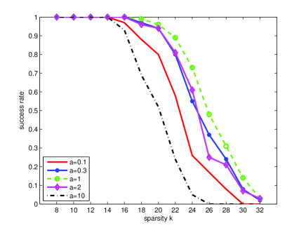
Figure 2: Numerical tests on parameter $a$ with $M=64$, $N=256$ by the unconstrained DCATL1 method.

We tested DCATL1 on recovering sparse vectors with different parameter $a$, varying among $\{0.1\ \ 0.3\ \ 1\ \ 2\ \ 10\}$. In this test, $A$ is a $64\times 256$ random matrix generated by normal Gaussian distribution. The true vector $x^{*}$ is also a randomly generated sparse vector with sparsity $k$ in the set $\{8\ \ 10\ \ 12\ ...\ \ 32\}$. Here the regularization parameter $\lambda$ was set to be $10^{-5}$ for all tests. Although the best $\lambda$ may be $k$-dependent in general, we considered the noiseless case and chose $\lambda=10^{-5}$ (small and fixed) to approximately enforce $Ax=Ax^{*}$. For each $a$, we sampled 100 times with different $A$ and $x^{*}$. The recovered vector $x_{r}$ is accepted and recorded as one success if the relative error: $\frac{\|x_{r}-x^{*}\|_{2}}{\|x^{*}\|_{2}}\leq 10^{-3}$.

Fig. 2 shows the success rate using DCATL1 over 100 independent trials for various values of parameter $a$ and sparsity $k$. From the figure, we see that DCATL1 with $a=1$ is the best among all tested values. Also numerical results for $a=0.3$ and $a=2$ (near 1), are better than those with 0.1 and 10. This is because the objective function is more non-convex at a smaller $a$ and thus more difficult to solve. On the other hand, iterations are more likely to stop at a local $\ell_{1}$ minima far from $\ell_{0}$ solution if $a$ is too large. Thus in all the following tests, we set the parameter $a=1$.

4.2 Numerical Experiment for Unconstrained Algorithm

The stopping conditions for outer loops are relative iteration error $\frac{\|x^{n+1}-x^{n}\|_{2}}{\|x^{n+1}\|_{2}}<10^{-5}$ and maximum iteration steps $20$. While, for the inner loop, the stopping condition are relative iteration error $10^{-8}$ and maximum iteration steps $5000$. The methods in comparison methods are applied with default parameters.

4.2.1 Gaussian matrix

We use $\mathcal{N}(0,\Sigma)$, the multi-variable normal distribution to generate Gaussian matrix $A$. Here covariance matrix is $\Sigma=\{(1-r)*\chi_{(i=j)}+r\}_{i,j}$, where the value of ‘$r$’ varies from 0 to 0.8. In theory, the larger the $r$ is, the more difficult it is to recover true sparse vector. For matrix $A$, the row number and column number are set to be $M=64$ and $N=1024$. The sparsity $k$ varies among $\{5\ \ 7\ \ 9\ ...\ \ 25\}$.

We compare four algorithms in terms of success rate. Denote $x_{r}$ as a reconstructed solution by a certain algorithm. We consider one algorithm to be successful, if the relative error of $x_{r}$ to the truth solution $x$ is less that 0.001, $i.e.$, $\frac{\|x_{r}-x\|_{2}}{\|x\|_{2}}<10^{-3}$. In order to improve success rates for all compared algorithms, we set tolerance parameter to be smaller or maximum cycle number to be higher inside each algorithm.

The success rate of each algorithm is plotted in Figure 3 with parameter $r$ from the set: $\{0\ \ 0.2\ \ 0.6\ \ 0.8\}$. For all cases, DCATL1 and reweighted $l_{1/2}$ algorithms (IRucLq-v) performed almost the same and both were much better than the other two, while the CEL0 has the lowest success rate.

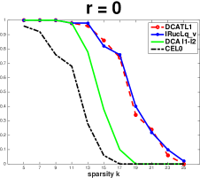
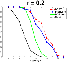
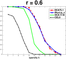
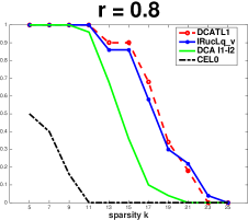
Figure 3: Numerical tests for unconstrained algorithms under Gaussian generated matrices: $M=64$, $N=1024$ with different coherence $r$.

4.2.2 Over-sampled DCT

The over-sampled DCT matrices [16, 23, 42] are:

$$\begin{array}[c]{l}A=[a_{1},...,a_{N}]\in\Re^{M\times N},\\ \ \ a_{j}=\dfrac{1}{\sqrt{M}}\cos(\dfrac{2\pi\omega(j-1)}{F}),\ \ j=1,...,N,\\ \text{ and $\omega$ is a random vector, drawn uniformly from $(0,1)^{M}$}.\end{array}$$ (4.1)

Such matrices appear as the real part of the complex discrete Fourier matrices in spectral estimation [16]. An important property is their high coherence: for a $100\times 1000$ matrix with $F=10$, the coherence is 0.9981, while the coherence of the same size matrix with $F=20$, is typically 0.9999.

The sparse recovery under such matrices is possible only if the non-zero elements of solution $x$ are sufficiently separated. This phenomenon is characterized as $minimum$ $separation$ in [7], and this minimum length is referred as the Rayleigh length (RL). The value of RL for matrix $A$ is equal to the factor $F$. It is closely related to the coherence in the sense that larger $F$ corresponds to larger coherence of a matrix. We find empirically that at least 2RL is necessary to ensure optimal sparse recovery with spikes further apart for more coherent matrices.

Under the assumption of sparse signal with 2RL separated spikes, we compare those four algorithms in terms of success rate. Denote $x_{r}$ as a reconstructed solution by a certain algorithm. We consider one algorithm successful, if the relative error of $x_{r}$ to the truth solution $x$ is less that $10^{-3}$, $i.e.$, $\frac{\|x_{r}-x\|_{2}}{\|x\|_{2}}<10^{-3}$. The success rate is averaged over 50 random realizations.

Fig. 4 shows success rates for those algorithms with increasing factor $F$ from 2 to 20. The sensing matrix is of size $100\times 1500$. It is interesting to see that along with the increasing of value $F$, DCA of $l_{1}-l_{2}$ algorithm performs better and better, especially after $F\geq 10$, and it has the highest success rate among all. Meanwhile, reweighted $l_{1/2}$ is better for low coherent matrices. When $F\geq 10$, it is almost impossible for it to recover sparse solution for the highly coherent matrix. Our DCATL1, however, is more robust and consistently performed near the top, sometimes even the best. So it is a valuable choice for solving sparse optimization problems where coherence of sensing matrix is unknown.

We further look at the success rates of DCATL1 with different combinations of sparsity and separation lengths for the over-sampled DCT matrix $A$. The rates are recorded in Table 1, which shows that when the separation is above with the minimum length, the sparsity relative to $M$ plays more important role in determining the success rates of recovery.

Table 1: The success rates (%) of DCATL1 for different combination of sparsity and minimum separation lengths.

sparsity	5	8	11	14	17	20
1RL	100	100	95	70	22	0
2RL	100	100	98	74	19	5
3RL	100	100	97	71	19	3
4RL	100	100	100	71	20	1
5RL	100	100	96	70	28	1

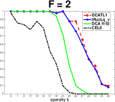
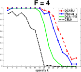
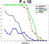
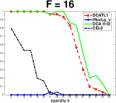
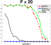
Figure 4: Numerical test for unconstrained algorithms under over-sampled DCT matrices: $M=100$, $N=1500$ with different $F$, and peaks of solutions separated by $2RL=2F$.

4.3 Numerical Experiment for Constrained Algorithm

For constrained algorithms, we performed similar numerical experiments. An algorithm is considered successful if the relative error of the numerical result $x_{r}$ from the ground truth $x$ is less than $10^{-3}$, or $\frac{\|x_{r}-x\|_{2}}{\|x\|_{2}}<10^{-3}$. We did 50 trials to compute average success rates for all the numerical experiments as for the unconstrained algorithms.

The stopping conditions for outer loop are relative iteration error $\frac{\|x^{n+1}-x^{n}\|_{2}}{\|x^{n+1}\|_{2}}<10^{-5}$ and maximum iteration steps $20$. While, for the inner loop, the stopping condition are relative iteration error $10^{-5}$ and maximum iteration steps $1000$. For other comparison methods, they are applied with default parameters.

4.3.1 Gaussian Random Matrices

We fix parameters $(M,N)=(64,1024)$, while covariance parameter $r$ is varied from 0 to 0.8. Comparison is with the reweighted $l_{1/2}$ and two $l_{1}$ algorithms (Bregman and yall1). In Fig. (5), we see that $Lp-RLS$ is the best among the four algorthms with DCATL1 trailing not much behind.

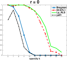
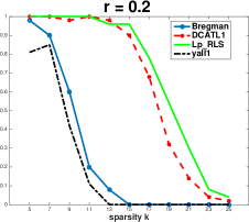
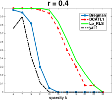
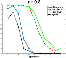
Figure 5: Comparison of constrained algorithms for $64\times 1024$ Gaussian random matrices with different coherence parameter $r$. The data points are averaged over 50 trials.

4.3.2 Over-sampled DCT

We fix $(M,N)=(100,1500)$, and vary parameter $F$ from 2 to 20, so the coherence of there matrices has a wider range and almost reaches 1 at the high end. In Fig. (6), when $F$ is small, say $F=2,4$, $Lp-RLS$ still performs the best, similar to the case of Gaussian matrices. However, with increasing $F$, the success rates for $Lp-RLS$ declines quickly, worse than the Bregman $l_{1}$ algorithm at $F=6,10$. The performance for DCATL1 is very stable and maintains a high level consistently even at the very high end of coherence ($F=20$).

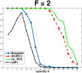
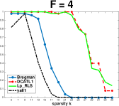
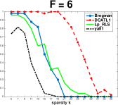
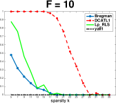
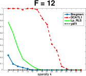
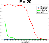
Figure 6: Comparison of success rates of constrained algorithms for the over-sampled DCT random matrices: $(M,N)=(100,1500)$ with different $F$ values, peak separation by $2RL=2F$.

Remark 4.1

In view of evaluation results in this section (Fig. 3, Fig. 4, Fig. 5, Fig. 6), we see that DCATL1 algorithms offer robust solutions in CS problems for random sensing matrices with a broad range of coherence. In applications where sensing hardwares cannot be modified or upgraded, a robust recovery algorithm is a valuable tool for information retrieval. An example is super-resolution where sparse signals are recovered from low frequency measurements within the hardware resolution limit [7, 22].

5 Comparison of DCA on Different Non-convex Penalties

In this section, we compare DCA on other non-convex penalty functions such as PiE [30], MCP [46], and SCAD [15]. The computation is based on our DCA-ADMM scheme, which uses Algorithm 1 to solve unconstrained optimization and Algorithm 2 to solve subproblems. The DCA schemes of these penalty functions are same as in [1, 30].

Among the three penalties, PiE has one hyperparameter while MCP and SCAD have two hyperparameters. We used $64\times 256$ Gaussian random matries to select best parameters for these penalties.

	Formula	Parameters
PiE	$\phi(t)=1-e^{-\beta|t|}$	$\beta=10$
MCP	$\phi(t)=\alpha\beta^{2}-\dfrac{[(\alpha\beta-|t|)_{+}]^{2}}{\alpha}$	$\alpha=5$, $\beta=0.1$
SCAD	$\phi(t)=\begin{cases}\beta|t|,&\mathrm{if}\ \ |t|\leq\beta;\\ -\dfrac{t^{2}-2\alpha\beta|t|+\beta^{2}}{2(\alpha-1)},&\mathrm{if}\ \ \beta<|t|\leq\alpha\beta;\\ \dfrac{(\alpha+1)\beta^{2}}{2},&\mathrm{if}\ \ |t|>\alpha\beta.\end{cases}$	$\alpha=5$, $\beta=0.1$

Table 2: Three non-convex penalty functions and their parameter values in the numerical experiments.

All other parameters for DCA algorithms during the numerical experiments are same as DCA-TL1. The success rate curves are shown in Fig. 7. DCA-MCP algorithm has very good performance on all Gaussian and over-sampled DCT matrices. In all the experiments, DCA-TL1 achieves almost the same level of success rates as DCA-MCP. Consistent with remark 2.2 and that the set of SCAD gNSP satisfying matrices is smaller than those of (PiE,TL1,MCP), SCAD is behind in the two plots of the first column of Fig. 7 where the sensing matrices are in the incoherent regime. Interestingly in the highly coherent regime (for over-sampled DCT matrices at $F=20$), DCA-SCAD fares well. From PiE behind MCP, TL1 in Fig. 7, and $\ell_{p}$ (in view of Fig. 3), the gNSP of PiE is likely to be more restrictive than those of MCP, TL1 and $\ell_{p}$, while the gNSP’s of the latter three are rather close. A precise characterization of these gNSP’s will be interesting for a future work.

It is worth pointing out that DCA-TL1 has only one hyperparameter and so is easier to adjust and adapt to different tasks. Two hyperparameters give more parameter space for improvement, but also require more efforts to search for optimal values.

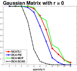
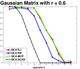
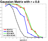
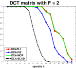
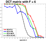
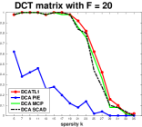
Figure 7: Numerical tests for DCA-ADMM scheme with different non-convex penalties using $64\times 1024$ random Gaussian matrices and $100\times 1500$ over-sampled DCT matrices of varying $(r,F)$ values.

6 Concluding Remarks

We have studied compressed sensing problems with the transformed $\ell_{1}$ penalty function (TL1) for both unconstrained and constrained models with random sensing matrices of a broad range of coherence. We discussed exact and stable recovery properties of TL1 using null space property and restricted isometry property of sensing matrices. We showed two DC algorithms along with a convergence theory.

In numerical experiments, DCATL1 with ADMM solving the convex sub-problems is on par with the best method reweighted $l_{1/2}$ ($Lp-RLS$) in the unconstrained (constrained) model, in case of incoherent Gaussian sensing matrices. For highly coherent over-sampled DCT random matrices, DCATL1 with ADMM solving the convex sub-problems is also comparable with the best method DCA $\ell_{1}-\ell_{2}$ algorithm. For random matrices of varying degree of coherence, the DCATL1 algorithm is the most robust for constrained and unconstrained models alike. We tested DCA with ADMM inner solver on other non-convex penalties (PiE, SCAD, MCP) with one and two hyperparameters, and found DCATL1 to be competitive as well.

In future work, we plan to develop TL1 algorithms for image processing and machine learning applications.

Appendix A Proof of Exact TL1 Sparse Recovery (Theorem 2.1)

Proof A.1.

The proof is along the lines of arguments in [4] and [9], while using special properties of the penalty function $\rho_{a}$. For simplicity, we denote $\beta_{C}$ by $\beta$ and $\beta^{0}_{C}$ by $\beta^{0}$.

Let $e=\beta-\beta^{0}$, and we want to prove that the vector $e=0$. It is clear that, $e_{T^{c}}=\beta_{T^{c}}$, since $T$ is the support set of $\beta^{0}$. By the triangular inequality of $\rho_{a}$, we have:

$$P_{a}(\beta^{0})-P_{a}(e_{T})=P_{a}(\beta^{0})-P_{a}(-e_{T})\leq P_{a}(\beta_{T}).$$

Then

$$\begin{array}[]{lll}P_{a}(\beta^{0})-P_{a}(e_{T})+P_{a}(e_{T^{c}})&\leq&P_{a}(\beta_{T})+P_{a}(\beta_{T^{c}})\\ &=&P_{a}(\beta)\\ &\leq&P_{a}(\beta^{0})\\ \end{array}$$

It follows that:

$$P_{a}(\beta_{T^{c}})=P_{a}(e_{T^{c}})\leq P_{a}(e_{T}).$$ (1.2)

Now let us arrange the components at $T^{c}$ in the order of decreasing magnitude of $|e|$ and partition into $L$ parts: $T^{c}=T_{1}\cup T_{2}\cup...\cup T_{L}$, where each $T_{j}$ has $R$ elements (except possibly $T_{L}$ with less). Also denote $T=T_{0}$ and $T_{01}=T\cup T_{1}$. Since $Ae=A(\beta-\beta^{0})=0$, it follows that

$$\begin{array}[]{lll}0&=&\|Ae\|_{2}\\ &=&\|A_{T_{01}}e_{T_{01}}+\sum\limits_{j=2}^{L}A_{T_{j}}e_{T_{j}}\|_{2}\\ &\geq&\|A_{T_{01}}e_{T_{01}}\|_{2}-\sum\limits_{j=2}^{L}\|A_{T_{j}}e_{T_{j}}\|_{2}\\ &\geq&\sqrt{1-\delta_{|T|+R}}\|e_{T_{01}}\|_{2}-\sqrt{1+\delta_{R}}\sum\limits_{j=2}^{L}\|e_{T_{j}}\|_{2}\end{array}$$ (1.3)

At the next step, we derive two inequalities between the $l_{2}$ norm and function $P_{a}$, in order to use the inequality (1.2). Since

$$\begin{array}[]{lll}\rho_{a}(|t|)=\dfrac{(a+1)|t|}{a+|t|}&\leq&(\dfrac{a+1}{a})|t|\\ &=&(1+\dfrac{1}{a})|t|\\ \end{array}$$

we have:

$$\begin{array}[]{lll}P_{a}(e_{T_{0}})&=&\sum\limits_{i\in T_{0}}\rho_{a}(|e_{i}|)\\ &\leq&(1+\frac{1}{a})\|e_{T_{0}}\|_{1}\\ &\leq&(1+\frac{1}{a})\sqrt{|T|}\ \ \|e_{T_{0}}\|_{2}\\ &\leq&(1+\frac{1}{a})\sqrt{|T|}\ \ \|e_{T_{01}}\|_{2}.\\ \end{array}$$ (1.4)

Now we estimate the $l_{2}$ norm of $e_{T_{j}}$ from above in terms of $P_{a}$. It follows from $\beta$ being the minimizer of the problem (2.12) and the definition of $x_{C}$ (2.9) that

$$P_{a}(\beta_{T^{c}})\leq P_{a}(\beta)\leq P_{a}(x_{C})\leq 1.$$

For each $i\in T^{c},\ \ \rho_{a}(\beta_{i})\leq P_{a}(\beta_{T^{c}})\leq 1$. Also since

$$\begin{array}[]{ll}&\dfrac{(a+1)|\beta_{i}|}{a+|\beta_{i}|}\leq 1\\ \Leftrightarrow&(a+1)|\beta_{i}|\leq a+|\beta_{i}|\\ \Leftrightarrow&|\beta_{i}|\leq 1\\ \end{array}$$ (1.5)

we have

$$|e_{i}|=|\beta_{i}|\leq\dfrac{(a+1)|\beta_{i}|}{a+|\beta_{i}|}=\rho_{a}(|\beta_{i}|)\ \ \ \mbox{for every $i\in T^{c}$}.$$

It is known that function $\rho_{a}(t)$ is increasing for non-negative variable $t\geq 0$, and

$$|e_{i}|\leq|e_{k}|\ \textit{ for }\ \forall\ i\in T_{j}\ \textit{ and }\ \forall\ k\in T_{j-1},$$

where $j=2,3,...,L$. Thus we have

$$\begin{array}[]{ll}\vspace{2mm}&|e_{i}|\leq\rho_{a}(|e_{i}|)\leq P_{a}(e_{T_{j-1}})/R\\ \vspace{2mm}\Rightarrow&\|e_{T_{j}}\|_{2}^{2}\leq\dfrac{P_{a}(e_{T_{j-1}})^{2}}{R}\\ \vspace{2mm}\Rightarrow&\|e_{T_{j}}\|_{2}\leq\dfrac{P_{a}(e_{T_{j-1}})}{R^{1/2}}\\ \vspace{2mm}\Rightarrow&\sum\limits_{j=2}^{L}\|e_{T_{j}}\|_{2}\leq\sum\limits_{j=1}^{L}\dfrac{P_{a}(e_{T_{j}})}{R^{1/2}}\\ \end{array}$$ (1.6)

Finally, plug (1.4) and (1.6) into inequality (1.3) to get:

$$\begin{array}[]{lll}\vspace{2mm}0&\geq&\sqrt{1-\delta_{|T|+R}}\dfrac{a}{(a+1)|T|^{1/2}}P_{a}(e_{T})-\sqrt{1+\delta_{R}}\dfrac{1}{R^{1/2}}P_{a}(e_{T})\\ \vspace{2mm}&\geq&\dfrac{P_{a}(e_{T})}{R^{1/2}}\left(\sqrt{1-\delta_{R+|T|}}\dfrac{a}{a+1}\sqrt{\dfrac{R}{|T|}}-\sqrt{1+\delta_{R}}\right)\end{array}$$ (1.7)

By the RIP condition (2.13), the factor $\sqrt{1-\delta_{R+|T|}}\dfrac{a}{a+1}\sqrt{\dfrac{R}{|T|}}-\sqrt{1+\delta_{R}}$ is strictly positive, hence $P_{a}(e_{T})=0$, and $e_{T}=0$. Also by inequality (1.2), $e_{T^{c}}=0$. We have proved that $\beta_{C}=\beta^{0}_{C}$. The equivalence of (2.12) and (2.11) holds. If another vector $\beta$ is the optimal solution of (2.12), we can prove that it is also equal to $\beta^{0}_{C}$, using the same procedure. Hence $\beta_{C}$ is unique.

Appendix B Proof of Stable TL1 Sparse Recovery (Theorem 2.2)

Proof B.1.

Set $n=A\beta-y_{C}$. We use three notations below:

• $\beta_{C}^{n}\Rightarrow$ optimal solution for the constrained problem (2.14);

• $\beta_{C}\Rightarrow$ optimal solution for the constrained problem (2.12);

• $\beta_{C}^{0}\Rightarrow$ optimal solution for the $l_{0}$ problem (2.11).

Let $T$ be the support set of $\beta_{C}^{0}$, i.e., $T=supp(\beta_{C}^{0})$, and vector $e=\beta_{C}^{n}-\beta_{C}^{0}$. Following the proof of Theorem 2.2, we obtain:

$$\sum\limits_{j=2}^{L}\|e_{T_{j}}\|_{2}\leq\sum\limits_{j=1}^{L}\frac{P_{a}(e_{T_{j}})}{R^{1/2}}=\frac{P_{a}(e_{T^{c}})}{R^{1/2}}$$

and

$$\|e_{T_{01}}\|_{2}\geq\frac{a}{(a+1)\sqrt{|T|}}P_{a}(e_{T}).$$

Further, due to the inequality $P_{a}(\beta_{T^{c}}^{n})=P_{a}(e_{T^{c}})\leq P_{a}(e_{T})$ from (1.2) and inequalities in (1.3), we get

$$\|Ae\|_{2}\geq\frac{P_{a}(e_{T})}{R^{1/2}}C_{\delta},$$

where $C_{\delta}=\sqrt{1-\delta_{R+|T|}}\dfrac{a}{a+1}\sqrt{\dfrac{R}{|T|}}-\sqrt{1+\delta_{R}}$.

By the initial assumption on the size of observation noise, we have

$$\|Ae\|_{2}=\|A\beta_{C}^{n}-A\beta_{C}^{0}\|_{2}=\|n\|_{2}\leq\tau,$$ (2.8)

so we have: $P_{a}(e_{T})\leq\dfrac{\tau R_{1/2}}{C_{\delta}}$.

On the other hand, we know that $P_{a}(\beta_{C})\leq 1$ and $\beta_{C}$ is in the feasible set of the problem (2.14). Thus we have the inequality: $P_{a}(\beta_{C}^{n})\leq P_{a}(\beta_{C})\leq 1$. By (1.5), $\beta_{C,i}^{n}\leq 1$ for each $i$. So, we have

$$|\beta_{C,i}^{n}|\leq\rho_{a}(|\beta_{C,i}^{n}|).$$ (2.9)

It follows that

$$\begin{array}[]{lll}\vspace{1mm}\|e\|_{2}&\leq&\|e_{T}\|_{2}+\|e_{T^{c}}\|_{2}=\|e_{T}\|_{2}+\|\beta_{C,T^{c}}^{n}\|_{2}\\ \vspace{1mm}&\leq&\dfrac{\|A_{T}e_{T}\|_{2}}{\sqrt{1-\delta_{T}}}+\|\beta_{C,T^{c}}^{n}\|_{1}\\ \vspace{1mm}&\leq&\dfrac{\|A_{T}e_{T}\|_{2}}{\sqrt{1-\delta_{T}}}+P_{a}(\beta_{C,T^{c}}^{n})=\dfrac{\|A_{T}e_{T}\|_{2}}{\sqrt{1-\delta_{T}}}+P_{a}(e_{T^{c}})\\ &\leq&\dfrac{\tau}{\sqrt{1-\delta_{R}}}+P_{a}(e_{T})\leq D\tau,\end{array}$$

for a positive constant $D$ depending only on $\delta_{R}$ and $\delta_{R+|T|}$. The second inequality uses the definition of RIP, while the first inequality in the last row comes from (2.8) and (1.2).

References

- [1] M. Ahn, J-S. Pang, and J. Xin, Difference-of-convex learning: directional stationarity, optimality, and sparsity SIAM Journal on Optimization 27 (3), 1637-1665, 2017
- [2] S. Boyd, N. Parikh, E. Chu, B. Peleato, and J. Eckstein, Distributed Optimization and Statistical Learning via the Alternating Direction Method of Multipliers, Foundations and Trends in Machine Learning, 3(1):1-122, 2011.
- [3] E. Candès, T. Tao, Decoding by linear programming, IEEE Trans. Info. Theory, 51(12):4203-4215, 2005.
- [4] E. Candès, M. Rudelson, T. Tao, R. Vershynin, Error correction via linear programming, in 46th Annual IEEE Symposium on Foundations of Computer Science, pp. 668-681, 2005.
- [5] E. Candès, J. Romberg, T. Tao, Robust uncertainty principles: Exact signal reconstruction from highly incomplete Fourier information, IEEE Trans. Info. Theory, 52(2), 489-509, 2006.
- [6] E. Candès, J. Romberg, T. Tao, Stable signal recovery from incomplete and inaccurate measurements, Comm. Pure Applied Mathematics, 59(8):1207-1223, 2006.
- [7] E. Candès, C. Fernandez-Granda, Super-resolution from noisy data, Journal of Fourier Analysis and Applications, 19(6):1229-1254, 2013.
- [8] W. Cao, J. Sun, and Z. Xu, Fast image deconvolution using closed-form thresholding formulas of regularization, Journal of Visual Communication and Image Representation, 24(1):31-41, 2013.
- [9] R. Chartrand, Nonconvex compressed sensing and error correction, ICASSP 2007, vol. 3, p. III 889.
- [10] R. Chartrand, W. Yin, Iteratively reweighted algorithms for compressive sensing, ICASSP 2008, pp. 3869-3872.
- [11] A. Cohen, W. Dahmen, R. DeVore, Compressed sensing and the best k-term approximation, J. Amer. Math. Soc., 22, pp. 211-231, 2009.
- [12] D. Donoho, Compressed sensing, IEEE Trans. Info. Theory, 52(4), 1289-1306, 2006.
- [13] D. Donoho, M. Elad, Optimally sparse representation in general (nonorthogonal) dictionaries via minimization, Proc. Nat. Acad. Scien. USA, vol. 100, pp. 2197-2202, 2003.
- [14] E. Esser, Y. Lou and J. Xin, A Method for Finding Structured Sparse Solutions to Non-negative Least Squares Problems with Applications, SIAM J. Imaging Sciences, 6(2013), pp. 2010-2046.
- [15] J. Fan, and R. Li, Variable selection via nonconcave penalized likelihood and its oracle properties, Journal of the American Statistical Association, 96(456):1348-1360, 2001.
- [16] A. Fannjiang, W. Liao, Coherence Pattern-Guided Compressive Sensing with Unresolved Grids, SIAM J. Imaging Sciences, Vol. 5, No. 1, pp. 179–202, 2012.
- [17] T. Goldstein and S. Osher, The Split Bregman Method for -regularized Problems, SIAM Journal on Imaging Sciences, 2(1):323-343, 2009.
- [18] M. Lai, Y. Xu, and W. Yin, Improved Iteratively Reweighted Least Squares for Unconstrained Smoothed Minimization, SIAM Journal on Numerical Analysis, 51(2):927-957, 2013.
- [19] H.A. Le Thi, B.T.A. Thi, and H.M. Le, Sparse signal recovery by difference of convex functions algorithms, Intelligent Information and Database Systems, pp. 387-397. Springer, 2013.
- [20] H.A. Le Thi, V. Ngai Huynh and T. Pham Dinh, DC programming and DCA for general DC programs, Advanced Computational Methods for Knowledge Engineering. Springer International Publishing, 2014. 15-35.
- [21] H.A. Le Thi, T. Pham Dinh, H.M. Le, and X.T. Vo, DC approximation approaches for sparse optimization, European Journal of Operational Research, 244.1 (2015): 26-46.
- [22] Y. Lou, P. Yin, and J. Xin, Point Source Super-resolution via Non-convex L1 Based Methods, J. Sci. Computing, 68(3), pp. 1082-1100, 2016.
- [23] Y. Lou, P. Yin, Q. He, and J. Xin, Computing Sparse Representation in a Highly Coherent Dictionary Based on Difference of L1 and L2, J. Scientific Computing, 64, 178–196, 2015.
- [24] Z. Lu and Y. Zhang, Sparse approximation via penalty decomposition methods, SIAM J. Optimization, 23(4):2448-2478, 2013.
- [25] J. Lv, and Y. Fan, A unified approach to model selection and sparse recovery using regularized least squares, Annals of Statistics, 37(6A), pp. 3498-3528, 2009.
- [26] S. Mallat and Z. Zhang, Matching pursuits with time-frequency dictionaries, IEEE Trans. Signal Processing, 41(12):3397-3415, 1993.
- [27] R. Mazumder, J. Friedman, and T. Hastie, SparseNet: Coordinate descent with nonconvex penalties, J. Amer. Stat. Assoc., 106(495):1125 1138, 2011.
- [28] B. Natarajan, Sparse approximate solutions to linear systems, SIAM Journal on Computing, 24(2):227-234, 1995.
- [29] D. Needell and R. Vershynin, Signal recovery from incomplete and inaccurate measurements via regularized orthogonal matching pursuit, IEEE Journal of Selected Topics in Signal Processing, 4(2):310-316, 2010.
- [30] T.B.T. Nguyen, H.A. Le Thi, H.M. Le and X.T. Vo, DC Approximation Approach for -minimization in Compressed Sensing, Advanced Computational Methods for Knowledge Engineering, 37-48, Springer, 2015.
- [31] M. Nikolova, Local strong homogeneity of a regularized estimator, SIAM Journal on Applied Mathematics 61(2), (2000): 633-658.
- [32] C.S. Ong, H.A. Le Thi, Learning sparse classifiers with difference of convex functions algorithms, Optimization Methods and Software, 28(4):830-854, 2013.
- [33] T. Pham Dinh and H.A. Le Thi, Convex analysis approach to d.c. programming: Theory, algorithms and applications, Acta Mathematica Vietnamica, vol. 22, no. 1, pp. 289-355, 1997.
- [34] T. Pham Dinh and H.A. Le Thi, A DC optimization algorithm for solving the trust-region subproblem, SIAM Journal on Optimization, 8(2), pp. 476–505, 1998.
- [35] E. Soubies, L. Blanc-Féraud, and G. Aubert, A Continuous Exact Penalty (CEL0) for Least Squares Regularized Problem, SIAM Journal on Imaging Sciences, 8.3 (2015): 1607-1639.
- [36] R. Tibshirani, Regression shrinkage and selection via the lasso, J. Royal. Statist. Soc, 58(1):267-288, 1996.
- [37] H. Tran, and C. Webster, Unified sufficient conditions for uniform recovery of sparse signals via nonconvex minimizations, arXiv:1701.07348, Oct. 19, 2017.
- [38] J. Tropp and A. Gilbert, Signal recovery from partial information via orthogonal matching pursuit, IEEE Trans. Inform. Theory, 53(12):4655-4666, 2007
- [39] F. Xu and S. Wang, A hybrid simulated annealing thresholding algorithm for compressed sensing, Signal Processing, 93:1577-1585, 2013.
- [40] Z. Xu, X. Chang, F. Xu, and H. Zhang, regularization: A thresholding representation theory and a fast solver, IEEE Transactions on Neural Networks and Learning Systems, 23(7):1013-1027, 2012.
- [41] J. Yang and Y. Zhang, Alternating direction algorithms for problems in compressive sensing, SIAM Journal on Scientific Computing, 33(1):250-278, 2011.
- [42] P. Yin, Y. Lou, Q. He, and J. Xin, Minimization of for compressed sensing, SIAM Journal on Scientific Computing, 37(1): A536 –A563, 2015.
- [43] P. Yin, and J. Xin, Iterative minimization for non-convex compressed sensing, J. Computational Mathematics, 35(4), 2017, pp. 437–449.
- [44] W. Yin, S. Osher, D. Goldfarb, and J. Darbon, Bregman iterative algorithms for -minimization with applications to compressed sensing, SIAM Journal on Imaging Sciences, 1(1):143-168, 2008.
- [45] J. Zeng, S. Lin, Y. Wang, and Z. Xu, regularization: Convergence of iterative half thresholding algorithm, IEEE Transactions on Signal Processing, 62(9):2317-2329, 2014.
- [46] C. Zhang, Nearly unbiased variable selection under minimax concave penalty, Ann. Statist., 38 (2010), pp. 894-942.
- [47] S. Zhang and J. Xin, Minimization of Transformed Penalty: Closed Form Representation and Iterative Thresholding Algorithms, Comm. Math Sci, 15(2), pp. 511–537, 2017.
- [48] S. Zhang, P. Yin, and J. Xin, Transformed Schatten-1 Iterative Thresholding Algorithms for Low Rank Matrix Completion, Comm. Math Sci, 15(3), pp. 839–862, 2017.