Forrelation: A Problem that Optimally Separates Quantum from Classical Computing

Abstract

We achieve essentially the largest possible separation between quantum and classical query complexities.  We do so using a property-testing problem called Forrelation, where one needs to decide whether one Boolean function is highly correlated with the Fourier transform of a second function.  This problem can be solved using $1$ quantum query, yet we show that any randomized algorithm needs $\Omega(\sqrt{N}/\log N)$ queries (improving an $\Omega(N^{1/4})$ lower bound of Aaronson).  Conversely, we show that this $1$ versus $\widetilde{\Omega}(\sqrt{N})$ separation is optimal: indeed, any $t$-query quantum algorithm whatsoever can be simulated by an $O\left(N^{1-1/2t}\right)$-query randomized algorithm.  Thus, resolving an open question of Buhrman et al. from 2002, there is no partial Boolean function whose quantum query complexity is constant and whose randomized query complexity is linear.  We conjecture that a natural generalization of Forrelation achieves the optimal $t$ versus $\Omega\left(N^{1-1/2t}\right)$ separation for all $t$.  As a bonus, we show that this generalization is $\mathsf{BQP}$-complete.  This yields what’s arguably the simplest $\mathsf{BQP}$-complete problem yet known, and gives a second sense in which Forrelation “captures the maximum power of quantum computation.”

1 Introduction

Since the work of Simon [23] and Shor [22] two decades ago, we have had powerful evidence that quantum computers can achieve exponential speedups over classical computers.  Of course, for problems like Factoring, these speedups are conjectural at present: we cannot rule out that a fast classical factoring algorithm might exist.  But in the black-box model, which captures most known quantum algorithms, exponential and even larger speedups can be proved.  We know, for example, that Period-Finding (a natural abstraction of the problem solved by Shor’s algorithm) is solvable with only $O\left(1\right)$ quantum queries, but requires $N^{\Omega\left(1\right)}$ classical randomized queries, where $N$ is the number of input elements [12, 10, 17].  We also know that Simon’s Problem is solvable with $O\left(\log N\right)$ quantum queries, but requires $\Omega(\sqrt{N})$ classical queries; and that a similar separation holds for the Glued-Trees problem introduced by Childs et al. [11, 16].

To us, these results raise an extremely interesting question:

• “The Speedup Question.”  Within the black-box model, just how large of a quantum speedup is possible?  For example, could there be a function of $N$ bits with a quantum query complexity of $1$, but a classical randomized query complexity of $\Omega\left(N\right)$?

One may object: once we know that exponential and even larger quantum speedups are possible in the black-box model, who cares about the exact limit?  In our view, the central reason to study the Speedup Question is that doing so can help us better understand the nature of quantum speedups themselves.  For example, can all exponential quantum speedups be seen as originating from a common cause?  Is there a single problem or technique that captures the advantages of quantum over classical query complexity, in much the same way that random sampling could be said to capture the advantages of randomized over deterministic query complexity?

As far as we know, the Speedup Question was first posed by Buhrman et al. [8] around 2002, in their study of quantum property-testing.  Specifically, Buhrman et al. asked whether there is any property of $N$-bit strings that exhibits a “maximal” separation: that is, one that requires $\Omega(N)$ queries to test classically, but only $O\left(1\right)$ quantumly.  The best separation they could find, based on Simon’s problem, was “deficient” on both ends: it required $\Omega(\sqrt{N})$ queries to test classically, and $O(\log N\log\log N)$ quantumly.

Since then, there has been only sporadic progress on the Speedup Question.  In 2009, Aaronson [1] introduced the Forrelation problem—a problem that we will revisit in this paper—and showed that it was solvable with only $1$ quantum query, but required $\Omega(N^{1/4})$ classical randomized queries.  In 2010, Chakraborty et al. [10] argued that Period-Finding gives a different example of an $O(1)$ versus $\widetilde{\Omega}(N^{1/4})$ quantum/classical gap; there, however, we only get an $O(1)$-query quantum algorithm if we allow non-Boolean queries.

Earlier, in 2001, de Beaudrap, Cleve, and Watrous [6] had given what they described as a black-box problem that was solvable with $1$ quantum query, but that required $\Omega(N^{1/4})$ or $\Omega(\sqrt{N})$ classical randomized queries (depending on how one defines the “input size” $N$).  However, de Beaudrap et al. were not working within the usual model of quantum query complexity.  Normally, one provides “black-box access” to a function $f$, meaning that the quantum algorithm can apply a unitary transformation that maps basis states of the form $\left|x,y\right\rangle$ to basis states of the form $\left|x,y\oplus f(x)\right\rangle$ (or $\left|x\right\rangle$ to $\left(-1\right)^{f\left(x\right)}\left|x\right\rangle$, if $f$ is Boolean).  By contrast, for their separation, de Beaudrap et al. had to assume the ability to map basis states of the form $\left|x,y\right\rangle$ to basis states of the form $\left|x,\pi(y+sx)\right\rangle$, for some unknown permutation $\pi$ and hidden shift $s$.

1.1 Our Results

This paper has two main contributions—the largest quantum black-box speedup yet known, and a proof that that speedup is essentially optimal—as well as many smaller related contributions.

1.1.1 Maximal Quantum/Classical Separation

In Section 4, we undertake a detailed study of the Forrelation problem, which Aaronson [1] introduced for a different purpose than the one that concerns us here (he was interested in an oracle separation between $\mathsf{BQP}$ and the polynomial hierarchy).  In Forrelation, we are given access to two Boolean functions $f,g:\left\{0,1\right\}^{n}\rightarrow\left\{-1,1\right\}$.  We want to estimate the amount of correlation between $f$ and the Fourier transform of $g$—that is, the quantity

$$\Phi_{f,g}:=\frac{1}{2^{3n/2}}\sum_{x,y\in\left\{0,1\right\}^{n}}f\left(x\right)\left(-1\right)^{x\cdot y}g\left(y\right).$$

It is not hard to see that $\left|\Phi_{f,g}\right|\leq 1$ for all $f,g$.  The problem is to decide, say, whether $\left|\Phi_{f,g}\right|\leq\frac{1}{100}$ or $\Phi_{f,g}\geq\frac{3}{5}$, promised that one of these is the case.  Here and throughout this paper, the “input size” is taken to be $N:=2^{n}$.

One can give (see Section 3) a quantum algorithm that solves Forrelation, with bounded probability of error, using only $1$ quantum query.  Intuitively, however, the property of $f$ and $g$ being “forrelated” (that is, having large $\Phi_{f,g}$ value) is an extremely global property, which should not be apparent to a classical algorithm until it has queried a significant fraction of the entire truth tables of $f$ and $g$.  And indeed, improving an $\Omega\left(N^{1/4}\right)$ lower bound of Aaronson [1], in Section 4 we show the following:

Theorem 1

Any classical randomized algorithm for Forrelation must make $\Omega(\frac{\sqrt{N}}{\log N})$ queries.

Theorem 1 yields the largest quantum versus classical separation yet known in the black-box model.  As we will show in Appendix 10, Theorem 1 also implies the largest property-testing separation yet known—for with some work, one can recast Forrelation (or rather, its negation) as a property that is testable with only $1$ query quantumly, but that requires $\Omega(\frac{\sqrt{N}}{\log N})$ queries to test classically.

We deduce Theorem 1 as a consequence of a more general result: namely, a lower bound on the classical query complexity of a problem called Gaussian Distinguishing.  Here we are given oracle access to a collection of $\mathcal{N}\left(0,1\right)$ real Gaussian random variables, $x_{1},\ldots,x_{M}$.  We are asked to decide whether the variables are all independent, or alternatively, whether they lie in a known low-dimensional subspace of $\mathbb{R}^{M}$: one that induces a covariance of at most $\varepsilon$ between each pair of variables, while keeping each variable an $\mathcal{N}\left(0,1\right)$ Gaussian individually.  We show the following:

Theorem 2

Gaussian Distinguishing requires $\Omega\left(\frac{1/\varepsilon}{\log(M/\varepsilon)}\right)$ classical randomized queries.

Theorem 1 is then simply a (discretized) special case of Theorem 2, with $M=2N$ and $\varepsilon=1/\sqrt{N}$.  Beyond that, it seems to us that Theorem 2 could have independent applications in statistics and machine learning.

1.1.2 Proof of Optimality

In Section 5, we show that the quantum/classical query complexity separation achieved by the Forrelation problem is close to the best possible.  More generally:

Theorem 3

Let $Q$ be any quantum algorithm that makes $t=O\left(1\right)$ queries to an $N$-bit string $X\in\left\{0,1\right\}^{N}$.  Then we can estimate $\Pr\left[Q\text{ accepts }X\right]$, to constant additive error and with high probability, by making only $O(N^{1-1/2t})$ classical randomized queries to $X$.  Moreover, the randomized queries are nonadaptive.

So for example, every $1$-query quantum algorithm can be simulated by an $O(\sqrt{N})$-query classical randomized algorithm, every $2$-query quantum algorithm can be simulated by an $O(N^{3/4})$-query randomized algorithm, and so on.  Theorem 3 resolves the open problem of Buhrman et al. [8] in the negative: it shows that there is no problem (property-testing or otherwise) with a constant versus linear quantum/classical query complexity gap.  Theorem 3 does not rule out the possibility of an $O\left(\log N\right)$ versus $\widetilde{\Omega}\left(N\right)$ gap, and indeed, we conjecture that such a gap is possible.

Once again, we deduce Theorem 3 as a consequence of a more general result, which might have independent applications to classical sublinear algorithms.  Namely:

Theorem 4

Every degree-$k$ real polynomial $p:\left\{-1,1\right\}^{N}\rightarrow\mathbb{R}$ that is

1. bounded in $\left[-1,1\right]$ at every Boolean point, and

2. “block-multilinear” (that is, the variables can be partitioned into $k$ blocks, such that every monomial is the product of one variable from each block),

can be approximated to within $\pm\varepsilon$, with high probability, by nonadaptively querying only $O(\left(N/\varepsilon^{2}\right)^{1-1/k})$ of the variables.

In the statement of Theorem 4, we strongly conjecture that condition (ii) can be removed.  If so, then we would obtain a sublinear algorithm to estimate any bounded, constant-degree real polynomial.  In Appendix 8, we show that condition (ii) can indeed be removed in the special case $k=2$.

1.1.3 $k$-fold Forrelation

In Section 6, we study a natural generalization of Forrelation.  In $k$-fold Forrelation, we are given access to $k$ Boolean functions $f_{1},\ldots,f_{k}:\left\{0,1\right\}^{n}\rightarrow\left\{-1,1\right\}$.  We want to estimate the “twisted sum”

$$\Phi_{f_{1},\ldots,f_{k}}:=\frac{1}{2^{\left(k+1\right)n/2}}\sum_{x_{1},\ldots,x_{k}\in\left\{0,1\right\}^{n}}f_{1}\left(x_{1}\right)\left(-1\right)^{x_{1}\cdot x_{2}}f_{2}\left(x_{2}\right)\left(-1\right)^{x_{2}\cdot x_{3}}\cdots\left(-1\right)^{x_{k-1}\cdot x_{k}}f_{k}\left(x_{k}\right).$$

It is not hard to show that $\left|\Phi_{f_{1},\ldots,f_{k}}\right|\leq 1$ for all $f_{1},\ldots,f_{k}$.  The problem is to decide, say, whether $\left|\Phi_{f_{1},\ldots,f_{k}}\right|\leq\frac{1}{100}$ or $\Phi_{f_{1},\ldots,f_{k}}\geq\frac{3}{5}$, promised that one of these is the case.

One can give (see Section 3) a quantum algorithm that solves $k$-fold Forrelation, with bounded error probability, using only $\left\lceil k/2\right\rceil$ quantum queries.  In Section 6, we show, conversely, that $k$-fold Forrelation “captures the full power of quantum computation”:

Theorem 5

If $f_{1},\ldots,f_{k}$ are described explicitly (say, by circuits to compute them), and $k=\operatorname*{poly}\left(n\right)$, then $k$-fold Forrelation is a $\mathsf{BQP}$-complete promise problem.

We do not know of any complete problem for quantum computation that is more self-contained than this.  Not only can one state the $k$-fold Forrelation problem without any notions from quantum mechanics, one does not need any nontrivial mathematical notions, like the condition number of a matrix or the Jones polynomial of a knot.

We conjecture, moreover, that $k$-fold Forrelation achieves the optimal $k/2$ versus $\widetilde{\Omega}(N^{1-1/k})$ quantum/classical query complexity separation for all even $k$.  If so, then there are two senses in which $k$-fold Forrelation captures the power of quantum computation.

1.1.4 Other Results

The paper also includes several other results.

In Appendix 7, we study the largest possible quantum/classical separations that are achievable for approximate sampling and relation problems.  We show that there exists a sampling problem—namely, Fourier Sampling of a Boolean function—that is solvable with $1$ quantum query, but requires $\Omega(N/\log N)$ classical queries.  By our previous results, this exceeds the largest quantum/classical gap that is possible for decision problems.

In Appendix 8, we generalize our result that every $1$-query quantum algorithm can be simulated using $O(\sqrt{N})$ randomized queries, to show that every bounded degree-$2$ real polynomial $p:\left\{-1,1\right\}^{N}\rightarrow\left[-1,1\right]$ can be estimated using $O(\sqrt{N})$ randomized queries.  We conjecture that this can be generalized, to show that every bounded degree-$k$ real polynomial can be estimated using $O(N^{1-1/k})$ randomized queries.

In Appendix 9, we extend our $\Omega(\frac{\sqrt{N}}{\log N})$ randomized lower bound for the Forrelation problem, to show a $\Omega(\frac{\sqrt{N}}{\log^{7/2}N})$ lower bound for $k$-fold Forrelation for any $k\geq 2$.  We conjecture that the right lower bound is $\widetilde{\Omega}(N^{1-1/k})$, but even generalizing our $\widetilde{\Omega}(\sqrt{N})$ lower bound to the $k$-fold case is nontrivial.

1.2 Techniques

1.2.1 Randomized Lower Bound

Proving that any randomized algorithm for Forrelation requires $\Omega(\frac{\sqrt{N}}{\log N})$ queries is surprisingly involved.  As we mentioned in Section 1.1.1, the first step, following the work of Aaronson [1], is to convert Forrelation into an analogous problem involving real Gaussian variables.  In Real Forrelation, we are given oracle access to two real functions $f,g:\left\{0,1\right\}^{n}\rightarrow\mathbb{R}$, and are promised either that (i) every $f\left(x\right)$ and $g\left(y\right)$ value is an independent $\mathcal{N}\left(0,1\right)$ Gaussian, or else (ii) every $f\left(x\right)$ value is an independent $\mathcal{N}\left(0,1\right)$ Gaussian, while every $g\left(y\right)$ value equals $\hat{f}\left(y\right)$ (i.e., the Fourier transform of $f$ evaluated at $y$).  The problem is to decide which holds.  Using a rounding reduction, we show that any query complexity lower bound for Real Forrelation implies the same lower bound for Forrelation itself.

Making the problem continuous allows us to adopt a geometric perspective.  In this perspective, we are given oracle access to a real vector $v\in\mathbb{R}^{2N}$, whose $2N$ coordinates consist of all values $f\left(x\right)$ and all values $g\left(y\right)$ (recall that $N=2^{n}$).  We are trying to distinguish the case where $v$ is simply an $\mathcal{N}\left(0,1\right)^{2N}$ Gaussian, from the case where $v$ is confined to an $N$-dimensional subspace of $\mathbb{R}^{2N}$—namely, the subspace defined by $g=\hat{f}$.  Now, suppose that values $f\left(x_{1}\right),\ldots,f\left(x_{t}\right)$ and $g\left(y_{1}\right),\ldots,g\left(y_{u}\right)$ have already been queried.  Then we can straightforwardly calculate the Bayesian posterior probabilities for being in case (i) or case (ii).  For case (i), the probability turns out to depend solely on the squared $2$-norm of the vector of empirical data seen so far:

$$\Pr\left[\text{case (i)}\right]\propto\exp\left(-\frac{\Delta_{\text{i}}}{2}\right),$$

where

$$\Delta_{\text{i}}=f\left(x_{1}\right)^{2}+\cdots+f\left(x_{t}\right)^{2}+g\left(y_{1}\right)^{2}+\cdots+g\left(y_{u}\right)^{2}.$$

For case (ii), by contrast, the probability is proportional to $\exp(-\Delta_{\text{ii}}/2)$, where $\Delta_{\text{ii}}$ is the minimum squared $2$-norm of any point $f\in\mathbb{R}^{N}$ compatible with all the data seen so far, as well as with the linear constraint $g=\hat{f}$.  Let $\mathcal{V}=\left\{\left|1\right\rangle,\ldots,\left|N\right\rangle,|\hat{1}\rangle,\ldots,|\hat{N}\rangle\right\}$ be the set of $2N$ unit vectors in $\mathbb{R}^{N}$ that consists of all $N$ elements of the standard basis, together with all $N$ elements of the Fourier basis.  Then $\Delta_{\text{ii}}$, in turn, can be calculated using a process of Gram-Schmidt orthogonalization, on the vectors in $\mathcal{V}$ corresponding to the $f$-values and $g$-values that have been queried so far.

Our goal is to show that, with high probability, $\Delta_{\text{i}}$ and $\Delta_{\text{ii}}$ remain close to each other, even after a large number of queries have been made—meaning that the algorithm has not yet succeeded in distinguishing case (i) from case (ii) with non-negligible bias.  To show this, the central fact we rely on is that the vectors in $\mathcal{V}$ are nearly-orthogonal: that is, for all $\left|v\right\rangle,\left|w\right\rangle\in\mathcal{V}$, we have $\left|\left\langle v|w\right\rangle\right|\leq\frac{1}{\sqrt{N}}$.  Intuitively, this means that, if we restrict attention to any small subset $S$ of  $f$-values and $g$-values, then while correlations exist among those values, the correlations are weak: “to a first approximation,” we have simply asked for the projections of a Gaussian vector onto $\left|S\right|$ orthogonal directions, and have therefore received $\left|S\right|$ uncorrelated answers.

From this perspective, the key question is: how many values can we query until the “orthogonal approximation” breaks down (meaning that we notice the correlations)?  In his previous work, Aaronson [1] showed that the approximation holds until $\Omega\left(N^{1/4}\right)$ queries are made.  Indeed, he proved a stronger statement: even if the $x$’s and $y$’s are chosen nondeterministically, still $\Omega\left(N^{1/4}\right)$ values must be revealed until we have a certificate showing that we are in case (i) or case (ii) with high probability.

To improve the lower bound from $\Omega\left(N^{1/4}\right)$ to the optimal $\widetilde{\Omega}(\sqrt{N})$, there are several hurdles to overcome.

Aaronson had assumed, conservatively, that the deviations from orthogonality all “pull in the same direction.”  As a first step, we notice instead that the deviations follow an unbiased random walk, with some positive and others negative—the martingale property arising from the fact that the algorithm can control which $x$’s and $y$’s to query, but not the values of $f\left(x\right)$ and $g\left(y\right)$.  We then use a Gaussian generalization of Azuma’s inequality to upper-bound the sum of the deviations.  Doing this improves the lower bound from $\Omega\left(N^{1/4}\right)$ to $\widetilde{\Omega}\left(N^{1/3}\right)$, but we then hit an apparent barrier.

In this work, we explain the $\Omega\left(N^{1/3}\right)$ barrier, by exhibiting a “model problem” that is extremely similar to Real Forrelation (in particular, has exactly the same near-orthogonality property), yet is solvable with only $O\left(N^{1/3}\right)$ queries, by exploiting adaptivity.  However, we then break the barrier, by using the fact that, for Real Forrelation (but not for the model problem), the total number of vectors in $\mathcal{V}$ is only $N^{O\left(1\right)}$.  This fact lets us use the Gaussian Azuma’s inequality a second time, to upper-bound not only the sum of all the deviations from orthogonality, but the individual deviations themselves.  Implementing this yields a lower bound of $\widetilde{\Omega}\left(N^{2/5}\right)$: better than $\widetilde{\Omega}\left(N^{1/3}\right)$, but still not all the way up to $\widetilde{\Omega}(\sqrt{N})$.  However, we then notice that we can apply Azuma’s inequality recursively—once for each layer of the Gram-Schmidt orthogonalization process—to get better and better upper bounds on the deviations from orthogonality.  Doing so gives us a sequence of lower bounds $\widetilde{\Omega}\left(N^{3/7}\right)$, $\widetilde{\Omega}\left(N^{4/9}\right)$, $\widetilde{\Omega}\left(N^{5/11}\right)$, etc., with the ultimate limit of the process being $\Omega(\frac{\sqrt{N}}{\log N})$.

1.2.2 Randomized Upper Bound

Why did we have to work so hard to prove a $\widetilde{\Omega}(\sqrt{N})$ lower bound on the randomized query complexity of Forrelation?  Our other main result provides one possible explanation: namely, we are here scraping up against the “ceiling” of the possible separations between randomized and quantum query complexity.  In particular, any quantum algorithm that makes $1$ query to a Boolean input $X\in\left\{0,1\right\}^{N}$, can be simulated by a randomized algorithm (in fact, a nonadaptive randomized algorithm) that makes $O(\sqrt{N})$ queries to $X$.  More generally, any quantum algorithm that makes $t=O\left(1\right)$ queries to $X$, can be simulated by a nonadaptive randomized algorithm that makes $O(N^{1-1/2t})$ queries to $X$.

The proof of this result consists of three steps.  The first involves the simulation of quantum algorithms by low-degree polynomials.  In 1998, Beals et al. [5] famously observed that, if a quantum algorithm makes $t$ queries to a Boolean input $X\in\left\{-1,1\right\}^{N}$, then $p\left(X\right)$, the probability that the algorithm accepts $X$, can be written as a multilinear polynomial in $X$ of degree at most $2t$.  We extend this result of Beals et al., in a way that might be of independent interest for quantum lower bounds.  Namely, we observe that every $t$-query quantum algorithm gives rise, not merely to a multilinear polynomial, but to a block-multilinear polynomial.  By this, we mean a degree-$2t$ polynomial $q$ that takes as input $2t$ blocks of $N$ variables each, and whose every monomial contains exactly one variable from each block.  If we repeat the input $X\in\left\{-1,1\right\}^{N}$ across all $2t$ blocks, then $q\left(X,\ldots,X\right)$ represents the quantum algorithm’s acceptance probability on $X$.  However, the key point is that $q\left(Y\right)$ is bounded in $\left[-1,1\right]$ for any Boolean input $Y\in\left\{-1,1\right\}^{2tN}$.

This leads to a new complexity measure for Boolean functions $f$: the block-multilinear approximate degree $\widetilde{\operatorname*{bmdeg}}\left(f\right)$, which lower-bounds the quantum query complexity $\operatorname*{Q}\left(f\right)$ just as $\widetilde{\deg}\left(f\right)$ does, but which might provide a tighter lower bound in some cases.  (Indeed, we do not even know whether there is any asymptotic separation between $\operatorname*{Q}\left(f\right)$ and $\widetilde{\operatorname*{bmdeg}}\left(f\right)$, whereas Ambainis [4] showed an asymptotic separation between $\operatorname*{Q}\left(f\right)$ and $\widetilde{\deg}\left(f\right)$.)

Once we have our quantum algorithm’s acceptance probability in the form of a block-multilinear polynomial $q$, the second step is to preprocess $q$, to make it easier to estimate using random sampling.  The basic problem is that $q$ might be highly “unbalanced”: certain variables might be hugely influential. Such variables are essential to query, but examining the form of $q$ does not make it obvious which variables these are.  To deal with this, we repeatedly perform an operation called “variable-splitting,” which consists of identifying an influential variable $x_{i}$, then replacing every occurrence of $x_{i}$ in $q$ by $\frac{1}{m}\left(x_{i,1}+\cdots+x_{i,m}\right)$, where $x_{i,1},\ldots,x_{i,m}$ are newly-created variables set equal to $x_{i}$.  The point of doing this is that each $x_{i,j}$ will be less influential in $q$ than $x_{i}$ itself was, thereby yielding a more balanced polynomial.  We show that variable-splitting can achieve the desired balance by introducing at most $\exp\left(t\right)\cdot O\left(N\right)$ new variables, which is linear in $N$ for constant $t$.

Once we have a balanced polynomial $q$, the last step is to give a query-efficient randomized algorithm to estimate its value.  Our algorithm is the simplest one imaginable: we simply choose $O(N^{1-1/2t})$ variables uniformly at random, query them, then form an estimate $\widetilde{q}$ of $q$ by summing only those monomials all of whose variables were queried.  The hard part is to prove that this estimator works—i.e., that its variance is bounded.  The proof of this makes heavy use of the balancedness property that was ensured by the preprocessing step.

Examining our estimation algorithm, an obvious question is whether it was essential that $q$ be block-multilinear, or whether the algorithm could be extended to all bounded low-degree polynomials.  In Appendix 8, we take a first step toward answering that question, by giving an $O(\sqrt{N})$-query randomized algorithm to estimate any bounded degree-$2$ polynomial in $N$ Boolean variables.  Once we drop block-multilinearity, our variable-splitting procedure no longer works, so we rely instead on Fourier-analytic results of Dinur et al. [14] to identify influential variables which we then split.

1.2.3 Other Results

$\mathsf{BQP}$-Completeness.  The proof that the $k$-fold Forrelation problem is $\mathsf{P{}romiseBQP}$-complete is simple, once one has the main idea.  The sum that defines $k$-fold Forrelation is, itself, an output amplitude for a particular kind of quantum circuit, which consists entirely of Hadamard and $f$-phase gates (i.e., gates that map $\left|x\right\rangle$ to $\left(-1\right)^{f\left(x\right)}\left|x\right\rangle$ for some Boolean function $f$).  Since the Hadamard and CCPHASE gates (corresponding to $f\left(x,y,z\right)=xyz$) are known to be universal for quantum computation, one might think that our work is done.  The difficulty is that the quantum circuit for $k$-fold Forrelation contains a Hadamard gate on every qubit, between every pair of $f$-phase gates, whether we wanted Hadamards there or not.  Thus, if we want to encode an arbitrary quantum circuit, then we need some way of canceling unwanted Hadamards, while leaving the wanted ones.  We achieve this via a gadget construction.

Separation for Sampling Problems.  To achieve a $1$ versus $\Omega(N/\log N)$ quantum/classical query complexity separation for a sampling problem, we consider Fourier Sampling: the problem, given oracle access to a Boolean function $f:\left\{0,1\right\}^{n}\rightarrow\left\{-1,1\right\}$, of outputting a string $y\in\left\{0,1\right\}^{n}$ with probability approximately equal to $\hat{f}\left(y\right)^{2}$.  This problem is trivially solvable with $1$ quantum query, but proving a $\Omega(N/\log N)$ classical lower bound takes a few pages of work.  The basic idea is to concentrate on the probability of a single string—say, $y=0^{n}$—being output.  Using a binomial calculation, we show that this probability cannot depend on $f$’s truth table in the appropriate way unless $\Omega(N/\log N)$ function values are queried.

Lower Bound for $\mathbf{k}$-Fold Forrelation.  Once we have a $\Omega(\frac{\sqrt{N}}{\log N})$ randomized lower bound for Forrelation, one might think it would be trivial to prove the same lower bound for $k$-fold Forrelation: just reduce one to the other!  However, Forrelation does not embed in any clear way as a subproblem of $k$-fold Forrelation.  On the other hand, given an instance of $k$-fold Forrelation, suppose we “give away for free” the complete truth tables of all but two of the functions.  In that case, we show that the induced subproblem on the remaining two functions is an instance of Gaussian Distinguishing to which, with high probability, our lower bound techniques can be applied.  Pursuing this idea leads to our $\Omega(\frac{\sqrt{N}}{\log^{7/2}N})$ lower bound on the randomized query complexity of $k$-fold Forrelation, for all $k\geq 2$.

Property-Testing Separation.  To turn our quantum versus classical separation for the Forrelation problem into a property-testing separation, we need to prove two interesting statements.  The first is that function pairs $\left\langle f,g\right\rangle$ that are far in Hamming distance from the set of all pairs with low forrelation, actually have high forrelation.  The second is that “generic” function pairs $\left\langle f,g\right\rangle$ and $\left\langle f^{\prime},g^{\prime}\right\rangle$ that have small Hamming distance from one another, are close in their forrelation values as well.  In fact, we will prove both of these statements for the general case of $k$-fold Forrelation.

1.3 Discussion

To summarize, this paper proves the largest separation between classical and quantum query complexities yet known, and it also proves that that separation is in some sense optimal. These results put us in a position to pose an intriguing open question:

Among all the problems that admit a superpolynomial quantum speedup, is there any whose classical randomized query complexity is $\gg\sqrt{N}$?

Strikingly, if we look at the known problems with superpolynomial quantum speedups, for every one of them the classical randomized lower bound seems to hit a “ceiling” at $\sqrt{N}$.  Thus, Simon’s Problem has quantum query complexity $O\left(\log N\right)$ and randomized query complexity $\widetilde{\Theta}(\sqrt{N})$; the Glued-Trees problem of Childs et al. [11] has quantum query complexity $\log^{O\left(1\right)}(N)$ and randomized query complexity $\widetilde{\Theta}(\sqrt{N})$; and Forrelation has quantum query complexity $1$ and randomized query complexity $\widetilde{\Theta}(\sqrt{N})$.

If we insist on making the randomized query complexity $\Omega(N^{1/2+c})$, for some $c>0$, and then try to minimize the quantum query complexity, then the best thing we know how to do is to take the OR of $N^{2c}$ independent instances of Forrelation, each of size $N^{1-2c}$.  This gives us a problem whose quantum query complexity is $\Theta(N^{c})$, and whose classical randomized query complexity is $\widetilde{\Theta}(N^{1/2+c})$.  Of course, this is not an exponential separation.

In this paper, we gave a candidate for a problem that breaks the “$\sqrt{N}$ barrier”: namely, $k$-fold Forrelation.  Indeed, we conjecture that $k$-fold Forrelation achieves the optimal separation for all $k=O\left(1\right)$, requiring $\widetilde{\Omega}\left(N^{1-1/k}\right)$ classical randomized queries but only $\left\lceil k/2\right\rceil$ quantum queries.  Proving this conjecture is an enticing problem.  Unfortunately, $k$-fold Forrelation becomes extremely hard to analyze when $k>2$, because we can no longer view the functions $f_{1},\ldots,f_{k}$ as confined to a low-dimensional subspace: now we have to view them as confined to a low-dimensional manifold, which is defined by degree-$\left(k-1\right)$ polynomials.  As such, we can no longer compute posterior probabilities by simply appealing to the rotational invariance of the Gaussian measure, which made our lives easier in the $k=2$ case.  Instead we need to calculate integrals over a nonlinear manifold.

Short of proving our conjecture about $k$-fold Forrelation, it would of course be nice to find any partial Boolean function whose quantum query complexity is $\operatorname*{polylog}N$, and whose randomized query complexity is $N^{1/2+\Omega\left(1\right)}$.

Another problem we leave is to generalize our $O\left(N^{1-1/k}\right)$ randomized estimation algorithm from block-multilinear polynomials to arbitrary bounded polynomials of degree $k$.  As we said, Appendix 8 achieves this in the special case $k=2$.  Achieving it for arbitrary $k$ seems likely to require generalizing the machinery of Dinur et al. [14].

A third problem concerns the notion of block-multilinear approximate degree, $\widetilde{\operatorname*{bmdeg}}\left(f\right)$, that we introduced to prove Theorem 4.  Is there any asymptotic separation between $\widetilde{\operatorname*{bmdeg}}\left(f\right)$ and ordinary approximate degree?  What about a separation between $\widetilde{\operatorname*{bmdeg}}\left(f\right)$ and quantum query complexity?

A fourth, more open-ended problem is whether there are any applications of Forrelation, in the same sense that factoring and discrete log provide “applications” of Shor’s period-finding problem.  Concretely, are there any situations where one has two efficiently-computable Boolean functions $f,g:\left\{0,1\right\}^{n}\rightarrow\left\{-1,1\right\}$ (described, for example, by circuits), one wants to estimate how forrelated they are, and the structure of $f$ and $g$ does not provide a fast classical way to do this?

Here are five other open problems:

1. Can we tighten the lower bound on the randomized query complexity of Forrelation from $\Omega(\frac{\sqrt{N}}{\log N})$ to $\Omega(\sqrt{N})$, or give an $O(\frac{\sqrt{N}}{\log N})$ upper bound?

2. Can we generalize our results from Boolean to non-Boolean functions?

3. What are the largest possible quantum versus classical query complexity separations for sampling problems?  Is an $O\left(1\right)$ versus $\Omega(N)$ separation possible in this case?  Also, what separations are possible for search or relation problems?  (For our results on these questions, see Appendix 7.)

4. While there exists a $1$-query quantum algorithm that solves Forrelation with bounded error probability, the error probability we are able to achieve is about $0.4$—more than the customary $1/3$.  If we want (say) a $1$ versus $N^{\Omega\left(1\right)}$ quantum versus classical query complexity separation, then how small can the quantum algorithm’s error be?

5. While we show in Appendix 10 that being “unforrelated”—that is, having $\Phi_{f,g}\leq\frac{1}{100}$—behaves nicely as a property-testing problem, it would be interesting to show the same for being forrelated.

2 Acknowledgments

We are grateful to Ronald de Wolf for early discussions, Andy Drucker for discussions about the randomized query complexity of $\operatorname*{OR}\left(f,\ldots,f\right)$, Shalev Ben-David and Sean Hallgren for discussions about the glued-trees problem, and Saeed Mehraban for a numerical calculation.

3 Preliminaries

We assume familiarity with basic concepts of quantum computing, as covered (for example) in Nielsen and Chuang [18].  We also assume some familiarity with the model of query or decision-tree complexity; see Buhrman and de Wolf [9] for a good survey.  In this section, we first give a brief recap of query complexity (in Section 3.1), then observe some properties of the $k$-fold Forrelation problem (in Section 3.2), and finally collect some lemmas about Gram-Schmidt orthogonalization (in Section 3.3) and Gaussian martingales (in Section 3.4) that will be important for our randomized lower bound in Section 4.

3.1 Query Complexity

Briefly, by the query complexity of an algorithm $\mathcal{A}$, we mean the number of queries that $\mathcal{A}$ makes to its input $z=\left(z_{1},\ldots,z_{N}\right)$, maximized over all valid inputs $z$.  The query complexity of a function $F$ is then the minimum query complexity of any algorithm $\mathcal{A}$ (of a specified type—classical, quantum, etc.) that outputs $F\left(z\right)$, with bounded probability of error, given any valid input $z$.

One slightly unconventional choice that we make is to define “bounded probability of error” to mean “error probability at most $1/2-\varepsilon$, for some constant $\varepsilon>0$” rather than “error probability at most $1/3$.”  The reason is that we will be able to design a $1$-query quantum algorithm that solves the Forrelation problem with error probability $2/5$, but not one that solves it with error probability $1/3$.  Of course, one can make the error probability as small as one likes using amplification, but doing so increases the query complexity by a constant factor.

We assume throughout this paper that the input $z\in\left\{-1,1\right\}^{N}$ is Boolean, and we typically work in the $\left\{-1,1\right\}$ basis for convenience.  In the classical setting, each query returns a single bit $z_{i}$, for some index $i\in\left[N\right]$ specified by $\mathcal{A}$.  In the quantum setting, each query performs a diagonal unitary transformation

$$\left|i,w\right\rangle\rightarrow z_{i}\left|i,w\right\rangle,$$

where $w$ represents “workspace qubits” that do not participate in the query.  Between two queries, $\mathcal{A}$ can apply any unitary transformation it likes that does not depend on $z$.

In this paper, the input $z=\left(z_{1},\ldots,z_{N}\right)$ will typically consist of the truth tables of one or more Boolean functions: for example, $f,g:\left\{0,1\right\}^{n}\rightarrow\left\{-1,1\right\}$, or $f_{1},\ldots,f_{k}:\left\{0,1\right\}^{n}\rightarrow\left\{-1,1\right\}$.  Throughout, we use $n$ for the number of input bits that these Boolean functions take (which roughly corresponds to the number of qubits in a quantum algorithm), and we use $N=2^{n}$ for the number of bits being queried in superposition.  (Strictly speaking, we should set $N=k\cdot 2^{n}$, where $k$ is the number of Boolean functions.  But this constant-factor difference will not matter for us.)  Thus, for the purposes of query complexity, $N$ is the “input size,” in terms of which we state our upper and lower bounds.

3.2 Forrelation

The Forrelation and $k$-fold Forrelation problems were defined in Sections 1.1.1 and 1.1.3 respectively.  Informally, though, one could define $k$-fold Forrelation simply as the problem of simulating the quantum circuit shown in Figure 1—and in particular, of estimating the amplitude, call it $\alpha_{0\cdots 0}$, with which this circuit returns $\left|0\right\rangle^{\otimes n}$ as its output.

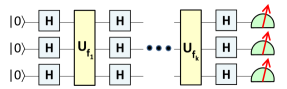
Figure 1: A quantum circuit that can be taken to define the $k$-fold Forrelation problem.  The circuit consists of $k$ query transformations $U_{f_{1}},\ldots,U_{f_{k}}$, which map each basis state $\left|x\right\rangle$ to $f_{i}\left(x\right)\left|x\right\rangle$, sandwiched between rounds of Hadamard gates.

Observe that $\alpha_{0\cdots 0}$ is precisely the quantity

$$\Phi_{f_{1},\ldots,f_{k}}:=\frac{1}{2^{\left(k+1\right)n/2}}\sum_{x_{1},\ldots,x_{k}\in\left\{0,1\right\}^{n}}f_{1}\left(x_{1}\right)\left(-1\right)^{x_{1}\cdot x_{2}}f_{2}\left(x_{2}\right)\left(-1\right)^{x_{2}\cdot x_{3}}\cdots\left(-1\right)^{x_{k-1}\cdot x_{k}}f_{k}\left(x_{k}\right)$$

defined in Section 1.1.3.  From this, it follows that we can decide whether $\left|\Phi_{f_{1},\ldots,f_{k}}\right|\leq\frac{1}{100}$ or $\Phi_{f_{1},\ldots,f_{k}}\geq\frac{3}{5}$ with bounded probability of error, and thereby solve the $k$-fold Forrelation problem, by making only $k$ quantum queries to $f_{1},\ldots,f_{k}$.

Slightly more interesting is that we can improve the quantum query complexity further, to $\left\lceil k/2\right\rceil$:

Proposition 6

The $k$-fold Forrelation problem is solvable, with error probability $0.4$, using $\left\lceil k/2\right\rceil$ quantum queries to the functions $f_{1},\ldots,f_{k}:\left\{0,1\right\}^{n}\rightarrow\left\{-1,1\right\}$, as well as $O\left(nk\right)$ quantum gates.

Proof. Let $\operatorname*{H}$ be the Hadamard gate, and let $U_{f_{i}}$ be the query transformation that maps each computational basis state $\left|x\right\rangle$ to $f_{i}\left(x\right)\left|x\right\rangle$.  Then to improve from $k$ to $\left\lceil k/2\right\rceil$ queries, we modify the circuit of Figure 1 in the following way.

In addition to the initial state $\left|0\right\rangle^{\otimes n}$, we prepare a control qubit in the state $\left|+\right\rangle=\frac{\left|0\right\rangle+\left|1\right\rangle}{\sqrt{2}}$.  Then, conditioned on the control qubit being $\left|0\right\rangle$, we apply the following sequence of operations to the initial state:

$$\operatorname*{H}\nolimits^{\otimes n}\rightarrow U_{f_{1}}\rightarrow\operatorname*{H}\nolimits^{\otimes n}\rightarrow U_{f_{2}}\rightarrow\cdots\rightarrow\operatorname*{H}\nolimits^{\otimes n}\rightarrow U_{f_{\left\lceil k/2\right\rceil}}\rightarrow\operatorname*{H}\nolimits^{\otimes n}.$$

Meanwhile, conditioned on the control qubit being $\left|1\right\rangle$, we apply the following sequence of operations:

$$\operatorname*{H}\nolimits^{\otimes n}\rightarrow U_{f_{k}}\rightarrow\operatorname*{H}\nolimits^{\otimes n}\rightarrow U_{f_{k-1}}\rightarrow\cdots\rightarrow\operatorname*{H}\nolimits^{\otimes n}\rightarrow U_{f_{\left\lceil k/2\right\rceil+1}}.$$

Finally, we measure the control qubit in the $\left\{\left|+\right\rangle,\left|-\right\rangle\right\}$ basis, and “accept” (i.e., say that $\Phi_{f_{1},\ldots,f_{k}}$ is large) if and only if we find it in the state $\left|+\right\rangle$.

It is not hard to see that the probability that this circuit accepts is exactly

$$\frac{1+\Phi_{f_{1},\ldots,f_{k}}}{2}.$$

Thus, consider an algorithm $\mathcal{A}$ that rejects with probability $1/4$, and runs the circuit with probability $3/4$.  We have

$$\Pr\left[\mathcal{A}\text{ accepts}\right]=\frac{3}{4}\left(\frac{1+\Phi_{f_{1},\ldots,f_{k}}}{2}\right).$$

If $\left|\Phi_{f_{1},\ldots,f_{k}}\right|\leq\frac{1}{100}$ then the above is less than $0.4$, while if $\Phi_{f_{1},\ldots,f_{k}}\geq\frac{3}{5}$ then it is at least $0.6$.   

Purely from the unitarity of the quantum algorithm to compute $\Phi_{f_{1},\ldots,f_{k}}$, we can derive some interesting facts about $\Phi_{f_{1},\ldots,f_{k}}$ itself.  Most obviously, we have $\left|\Phi_{f_{1},\ldots,f_{k}}\right|\leq 1$.  But beyond that, let $f_{k}^{\left(x\right)}\left(x_{k}\right):=f_{k}\left(x_{k}\right)\left(-1\right)^{x_{k}\cdot x}$.  Then

$$\sum_{x\in\left\{0,1\right\}^{n}}\Phi_{f_{1},\ldots,f_{k-1},f_{k}^{\left(x\right)}}^{2}=1;$$ (1)

this is just saying that the sum of the squares of the final amplitudes in the Forrelation algorithm must be $1$.  Since there is nothing “special” about the outcome $\left|0\cdots 0\right\rangle$, it follows by symmetry that

$$\operatorname*{E}\left[\Phi_{f_{1},\ldots,f_{k}}^{2}\right]=\frac{1}{N}$$

if $f_{1},\ldots,f_{k}$ are chosen are uniformly at random.

3.3 Gram-Schmidt Orthogonalization

Given an arbitrary collection of linearly-independent unit vectors $\left|v_{1}\right\rangle,\left|v_{2}\right\rangle\ldots$, the Gram-Schmidt process produces orthonormal vectors by recursively projecting each $\left|v_{i}\right\rangle$ onto the orthogonal complement of the subspace spanned by $\left|v_{1}\right\rangle,\ldots,\left|v_{i-1}\right\rangle$, and then normalizing the result.  That is:

$$\left|z_{i}\right\rangle =\left|v_{i}\right\rangle-\sum_{j=1}^{i-1}\left\langle v_{i}|w_{j}\right\rangle\left|w_{j}\right\rangle,$$

$$\left|w_{i}\right\rangle =\beta_{i}\left|z_{i}\right\rangle$$

where $\beta_{i}=\frac{1}{\sqrt{\left\langle z_{i}|z_{i}\right\rangle}}$ is a normalizing constant.  Note that $\left\langle z_{i}|z_{i}\right\rangle\leq 1$ (since $\left|z_{i}\right\rangle$ is the projection of a unit vector onto a subspace), and hence $\beta_{i}\geq 1$.

We will be interested in the behavior of this process when the $\left|v_{i}\right\rangle$’s are already very close to orthogonal.  We can control that behavior with the help of the following lemma.

Lemma 7 (Gram-Schmidt Lemma)

Let $\left|v_{1}\right\rangle,\ldots,\left|v_{t}\right\rangle$ be unit vectors with $\left|\left\langle v_{i}|v_{j}\right\rangle\right|\leq\varepsilon$ for all $i\neq j$, and suppose $t\leq 0.1/\varepsilon$ (so in particular, $\varepsilon\leq 0.1$).  Let $\left|w_{i}\right\rangle$ and $\beta_{i}$ be as above.  Then for all $i>j$, we have

$$\left|\left\langle v_{i}|w_{j}\right\rangle\right| \leq\varepsilon+2j\varepsilon^{2},$$

$$\beta_{i} \leq 1+2i\varepsilon^{2}.$$

So in particular, under the stated hypothesis, $\left|\left\langle v_{i}|w_{j}\right\rangle\right|\leq 1.2\varepsilon$ and $\beta_{i}\leq 1+0.2\varepsilon$.

Proof. We will do an induction on ordered pairs $\left(i,j\right)$, in the order $\left(2,1\right),\left(3,1\right),\left(3,2\right),\left(4,1\right),\ldots$, with two induction hypotheses.  Here are the hypotheses: for all $i>j$,

$$\left|\left\langle v_{i}|w_{j}\right\rangle\right| \leq\varepsilon+Aj\varepsilon^{2},$$

$$1-\left\langle z_{i}|z_{i}\right\rangle \leq Bi\varepsilon^{2}.$$

for some constants $A,B$ to be determined later.

For the base case ($i=2$ and $j=1$), we have $\left|\left\langle v_{2}|w_{1}\right\rangle\right|=\left|\left\langle v_{2}|v_{1}\right\rangle\right|\leq\varepsilon$ and

$$\left\langle z_{2}|z_{2}\right\rangle =\left(\left\langle v_{2}\right|-\left\langle v_{1}|v_{2}\right\rangle\left\langle v_{1}\right|\right)\left(\left|v_{2}\right\rangle-\left\langle v_{1}|v_{2}\right\rangle\left|v_{1}\right\rangle\right)$$

$$=1-\left\langle v_{1}|v_{2}\right\rangle^{2}$$

$$\geq 1-\varepsilon^{2}.$$

For the induction step: first,

$$\left\langle v_{i}|w_{j}\right\rangle =\left\langle v_{i}\right|\beta_{j}\left(\left|v_{j}\right\rangle-\sum_{k=1}^{j-1}\left\langle v_{j}|w_{k}\right\rangle\left|w_{k}\right\rangle\right)$$

$$=\frac{1}{\sqrt{\left\langle z_{j}|z_{j}\right\rangle}}\left(\left\langle v_{i}|v_{j}\right\rangle+\sum_{k=1}^{j-1}\left\langle v_{i}|w_{k}\right\rangle\left\langle v_{j}|w_{k}\right\rangle\right).$$

So

$$\left|\left\langle v_{i}|w_{j}\right\rangle\right| \leq\frac{1}{\sqrt{1-Bj\varepsilon^{2}}}\left(\varepsilon+\sum_{k=1}^{j-1}\left(\varepsilon+Ak\varepsilon^{2}\right)^{2}\right)$$

$$\leq\frac{1}{1-Bj\varepsilon^{2}}\left(\varepsilon+j\varepsilon^{2}+Aj^{2}\varepsilon^{3}+\frac{A^{2}j^{3}\varepsilon^{4}}{3}\right)$$

$$\leq\left(1+\frac{B}{1-0.01B}j\varepsilon^{2}\right)\left(\varepsilon+\left(1+0.1A+\frac{0.01A^{2}}{3}\right)j\varepsilon^{2}\right)$$

$$\leq\varepsilon+\left[\left(1+0.1A+\frac{0.01A^{2}}{3}\right)\left(1+\frac{0.01B}{1-0.01B}\right)+\frac{0.1B}{1-0.01B}\right]j\varepsilon^{2},$$

where we repeatedly made the substitutions $\varepsilon\leq 0.1$ and $j\varepsilon\leq 0.1$ to produce multiples of $j\varepsilon^{2}$ in the numerator, and get rid of $j$ and $\varepsilon$ in the denominator.  Second,

$$\left\langle z_{i}|z_{i}\right\rangle =\left(\left\langle v_{i}\right|-\sum_{j=1}^{i-1}\left\langle v_{i}|w_{j}\right\rangle\left\langle w_{j}\right|\right)\left(\left|v_{i}\right\rangle-\sum_{j=1}^{i-1}\left\langle v_{i}|w_{j}\right\rangle\left|w_{j}\right\rangle\right)$$

$$=\left\langle v_{i}|v_{i}\right\rangle-\sum_{j=1}^{i-1}\left\langle v_{i}|w_{j}\right\rangle^{2}+\sum_{j\neq k\in\left[i-1\right]}\left\langle v_{i}|w_{j}\right\rangle\left\langle v_{i}|w_{k}\right\rangle\left\langle w_{j}|w_{k}\right\rangle$$

$$=1-\sum_{j=1}^{i-1}\left\langle v_{i}|w_{j}\right\rangle^{2}$$

where we used the fact that $\left\langle w_{j}|w_{k}\right\rangle=0$.  So

$$1-\left\langle z_{i}|z_{i}\right\rangle \leq\sum_{j=1}^{i-1}\left(\varepsilon+Aj\varepsilon^{2}\right)^{2}$$

$$\leq i\varepsilon^{2}+Ai^{2}\varepsilon^{3}+\frac{A^{2}i^{3}\varepsilon^{4}}{3}$$

$$\leq\left(1+0.1A+\frac{0.01A^{2}}{3}\right)i\varepsilon^{2}.$$

If we now make the choice (say) $A=2$ and $B=1.5$, we find that both parts of the induction are satisfied:

$$\left|\left\langle v_{i}|w_{j}\right\rangle\right| \leq\varepsilon+1.39j\varepsilon^{2}\leq\varepsilon+Aj\varepsilon^{2},$$

$$1-\left\langle z_{i}|z_{i}\right\rangle \leq 1.22i\varepsilon^{2}\leq Bi\varepsilon^{2}.$$

Furthermore, we now have the lemma, since

$$\beta_{i}=\frac{1}{\sqrt{\left\langle z_{i}|z_{i}\right\rangle}}\leq\frac{1}{\left\langle z_{i}|z_{i}\right\rangle}=1+\frac{1-\left\langle z_{i}|z_{i}\right\rangle}{\left\langle z_{i}|z_{i}\right\rangle}\leq 1+\frac{Bi\varepsilon^{2}}{1-Bi\varepsilon^{2}}\leq 1+\frac{Bi\varepsilon^{2}}{1-0.01B}\leq 1+2i\varepsilon^{2}.$$

 

3.4 Gaussian Azuma’s Inequality

Azuma’s inequality is a well-known generalization of the Chernoff/Hoeffing tail bound to the case of martingales with bounded differences.  We will need a generalization of Azuma’s inequality to martingale difference sequences in which each term is Gaussian (and therefore, unbounded).  Fortunately, Shamir [20, Theorem 2] recently proved a useful such generalization.  We now state Shamir’s bound, in a slightly different form than in [20] (but easily seen to be equivalent).

Lemma 8 (Gaussian Azuma’s Inequality [20])

Suppose $x_{1},x_{2},\ldots$ form a martingale difference sequence, in the sense that $\operatorname{E}\left[x_{i}|x_{1},\ldots,x_{i-1}\right]=0$.  Suppose further that, conditioned on its predecessors, $x_{i}$ is always “dominated by an $\mathcal{N}\left(0,\sigma^{2}\right)$ Gaussian,” in the sense that $\Pr\left[\left|x_{i}\right|>\sigma B\right]<\exp\left(-B^{2}/2\right)$ for all $B$.  Then

$$\Pr\left[\left|x_{1}+\cdots+x_{t}\right|>c\sigma\sqrt{t}\right]<2\exp\left(-\frac{c^{2}}{56}\right).$$

Note, in particular, that if the $x_{i}$’s themselves are $\mathcal{N}\left(0,\tau_{i}^{2}\right)$ Gaussians for some (possibly-differing) variances $\tau_{i}<\sigma$, then the $x_{i}$’s are dominated by $\mathcal{N}\left(0,\sigma^{2}\right)$ Gaussians, so Lemma 8 can be applied.

4 Maximal Quantum/Classical Query Complexity Gap

In this section, we prove that the randomized query complexity of Forrelation is $\Omega(\frac{\sqrt{N}}{\log N})$.  Previously, Aaronson [1] proved an $\Omega(N^{1/4})$ randomized lower bound for this problem.  We will need a further idea to improve the lower bound to $\widetilde{\Omega}(N^{1/3})$, a still further idea to improve it to $\widetilde{\Omega}(N^{2/5})$, and then yet another idea to get all the way up to $\widetilde{\Omega}(\sqrt{N})$.

Following [1], the first step is to replace Forrelation by a “continuous relaxation” of the problem: a version that is strictly easier (and thus, for which proving a lower bound is harder), but which has rotational symmetry that will be extremely convenient for us.  Thus, in Real Forrelation, we are given oracle access to two real functions $f,g:\left\{0,1\right\}^{n}\rightarrow\mathbb{R}$.  As usual, the “input size” is $N=2^{n}$.  We are promised that the pair $\left\langle f,g\right\rangle$ was drawn from one of two probability measures:

1. In the uniform measure $\mathcal{U}$, every $f\left(x\right)$ and $g\left(y\right)$ value is an independent $\mathcal{N}\left(0,1\right)$ Gaussian.

2. In the forrelated measure $\mathcal{F}$, every $f\left(x\right)$ value is an independent $\mathcal{N}\left(0,1\right)$ Gaussian, while every $g\left(y\right)$ value is fixed to

   $$\hat{f}\left(y\right)=\frac{1}{\sqrt{N}}\sum_{x\in\left\{0,1\right\}^{n}}\left(-1\right)^{x\cdot y}f\left(x\right).$$

The problem is to decide, with constant bias, whether (i) or (ii) holds (i.e., whether $\left\langle f,g\right\rangle$ was drawn from $\mathcal{U}$ or from $\mathcal{F}$).

We will often treat (the truth tables of) $f$ and $g$ as vectors in $\mathbb{R}^{N}$.  Then another way to think about Real Forrelation is this: in case (i), $f$ and $g$ are drawn independently from $\mathcal{N}\left(0,1\right)^{N}$.  In case (ii), $f$ and $g$ are also both distributed according to $\mathcal{N}\left(0,1\right)^{N}$, by the rotational symmetry of the Gaussian measure and the unitarity of the Hadamard transform.  But they are no longer independent: they are related by $g=Hf$, where $H$ is the $N\times N$ Hadamard matrix, given by $H_{x,y}=\left(-1\right)^{x\cdot y}/\sqrt{N}$.  The problem is to detect whether this correlation is present.

An algorithm for Real Forrelation proceeds by querying $f\left(x\right)$ and $g\left(y\right)$ values one at a time, deciding which $x$ or $y$ to query next based on the values seen so far.  We are interested in the expected number of queries needed by the best algorithm.

4.1 Discrete Versus Continuous

As a first step, we need to show that a lower bound for Real Forrelation really does imply the same lower bound for the original, Boolean Forrelation problem.  The key to doing so is the following result, which calculates the expected value of $\Phi_{F,G}$, for Boolean Forrelation instances $\left\langle F,G\right\rangle$ that are produced by “rounding” real instances $\left\langle f,g\right\rangle$ in a natural way.

Theorem 9

Suppose $\left\langle f,g\right\rangle$ are drawn from the forrelated measure $\mathcal{F}$.  Define Boolean functions $F,G:\left\{0,1\right\}^{n}\rightarrow\left\{-1,1\right\}$ by $F\left(x\right):=\operatorname*{sgn}\left(f\left(x\right)\right)$ and $G\left(y\right):=\operatorname*{sgn}\left(g\left(y\right)\right)$.  Then

$$\operatorname{E}_{f,g\sim\mathcal{F}}\left[\Phi_{F,G}\right]=\frac{2}{\pi}\pm O\left(\frac{\log N}{N}\right).$$

Proof. By linearity of expectation, it suffices to calculate $\operatorname{E}\left[F\left(x\right)\left(-1\right)^{x\cdot y}G\left(y\right)\right]$ for some specific $x,y$ pair.  Let $v\in\mathbb{R}^{N}$ be a vector of independent $\mathcal{N}\left(0,1\right)$ Gaussians, and let $H$ be the $N\times N$ Hadamard matrix (without normalization), with entries $H_{x,y}=\left(-1\right)^{x\cdot y}$.  Then we can consider $\left\langle F,G\right\rangle$ to have been generated as follows:

$$F\left(x\right) =\operatorname*{sgn}\left(v_{x}\right),$$

$$G\left(y\right) =\operatorname*{sgn}(\left(Hv\right)_{y}).$$

Now, $\left(Hv\right)_{y}$ can be expressed as the sum of $H_{x,y}v_{x}$ with the independent Gaussian random variable

$$Z:=\sum_{x^{\prime}\neq x}H_{x^{\prime},y}v_{x^{\prime}}.$$

Let $G^{\prime}\left(y\right):=\operatorname*{sgn}\left(Z\right)$.  Then

$$\operatorname{E}\left[F\left(x\right)\left(-1\right)^{x\cdot y}G^{\prime}\left(y\right)\right]=\operatorname{E}\left[\operatorname*{sgn}\left(v_{x}\right)\left(-1\right)^{x\cdot y}\operatorname*{sgn}\left(Z\right)\right]=0,$$

since $v_{x}$ and $Z$ are independent Gaussians both with mean $0$.  Note that adding $H_{x,y}v_{x}$ back to $Z$ can only flip $Z$ to having the same sign as $\operatorname*{sgn}\left(v_{x}\right)\left(-1\right)^{x\cdot y}$, not the opposite sign—and hence can only increase $F\left(x\right)\left(-1\right)^{x\cdot y}G\left(y\right)$.  It follows that

$$\operatorname{E}\left[F\left(x\right)\left(-1\right)^{x\cdot y}G\left(y\right)\right]=2\Pr\left[G\left(y\right)\neq G^{\prime}\left(y\right)\right].$$

The event $G\left(y\right)\neq G^{\prime}\left(y\right)$ occurs if and only if the following two events both occur:

$$\left|H_{x,y}v_{x}\right| >\left|Z\right|,$$

$$\operatorname*{sgn}\left(H_{x,y}v_{x}\right) \neq\operatorname*{sgn}\left(Z\right).$$

Since $H_{x,y}\in\left\{-1,1\right\}$ and the distribution of $v_{x}$ is symmetric about $0$, we can assume without loss of generality that $H_{x,y}=1$.

Let $Z\left(t\right)$ be the probability density function of $Z$.  Then

$$\Pr\left[\left|H_{x,y}v_{x}\right|>\left|Z\right|\text{ \ and \ }\operatorname*{sgn}\left(H_{x,y}v_{x}\right)\neq\operatorname*{sgn}\left(Z\right)\right] =2\int_{t=0}^{\infty}Z\left(t\right)\Pr\left[H_{x,y}v_{x}>t\right]dt$$

$$=2\int_{t=0}^{\infty}Z\left(t\right)\Pr\left[v_{x}>t\right]dt.$$

(Here the factor of $2$ appears because we are restricting to the case $Z>0$, and there is an equal probability coming from the $Z<0$ case.)

As a linear combination of $N-1$ independent $\mathcal{N}\left(0,1\right)$ Gaussians, with $\pm 1$ coefficients, $Z$ has the $\mathcal{N}\left(0,N-1\right)$ Gaussian distribution.  Therefore

$$2\int_{t=0}^{\infty}Z\left(t\right)\Pr\left[v_{x}>t\right]dt =\frac{2}{\sqrt{2\pi\left(N-1\right)}}\int_{t=0}^{\infty}\exp\left(-\frac{t^{2}}{2\left(N-1\right)}\right)\Pr\left[v_{x}>t\right]dt$$

$$\leq\frac{2}{\sqrt{2\pi\left(N-1\right)}}\int_{t=0}^{\infty}\Pr\left[v_{x}>t\right]dt$$

$$=\frac{2}{\sqrt{2\pi\left(N-1\right)}}\operatorname{E}\left[\left|v_{x}\right|\right]$$

$$=\frac{2}{\pi\sqrt{N-1}}$$

$$\leq\frac{2}{\pi\sqrt{N}}+O\left(\frac{1}{N^{3/2}}\right).$$

Here the fourth line follows from $\operatorname{E}\left[\left|X\right|\right]=\sqrt{2/\pi}$ when $X$ is an $\mathcal{N}\left(0,1\right)$ Gaussian.  In the other direction, for all $C>0$ we have

$$2\int_{t=0}^{\infty}Z\left(t\right)\Pr\left[v_{x}>t\right]dt =\frac{2}{\sqrt{2\pi\left(N-1\right)}}\int_{t=0}^{\infty}\exp\left(-\frac{t^{2}}{2\left(N-1\right)}\right)\Pr\left[v_{x}>t\right]dt$$

$$\geq\frac{2}{\sqrt{2\pi N}}\int_{t=0}^{C}\exp\left(-\frac{t^{2}}{2\left(N-1\right)}\right)\Pr\left[v_{x}>t\right]dt$$

$$\geq\frac{2}{\sqrt{2\pi N}}\exp\left(-\frac{C^{2}}{2\left(N-1\right)}\right)\int_{t=0}^{C}\Pr\left[v_{x}>t\right]dt$$

$$=\frac{2}{\sqrt{2\pi N}}\exp\left(-\frac{C^{2}}{2\left(N-1\right)}\right)\left(\operatorname{E}\left[\left|v_{x}\right|\right]-\frac{1}{\sqrt{2\pi}}\int_{t=C}^{\infty}te^{-t^{2}/2}dt\right)$$

$$=\frac{2}{\sqrt{2\pi N}}\exp\left(-\frac{C^{2}}{2\left(N-1\right)}\right)\left(\sqrt{\frac{2}{\pi}}-\frac{e^{-C^{2}/2}}{\sqrt{2\pi}}\right).$$

If we set $C:=\sqrt{\log N}$, then the above is

$$\frac{2}{\sqrt{2\pi N}}\left(1-O\left(\frac{\log N}{N}\right)\right)\left(\sqrt{\frac{2}{\pi}}-\frac{1}{\sqrt{2\pi}N}\right)\geq\frac{2}{\pi\sqrt{N}}-O\left(\frac{\log N}{N^{3/2}}\right).$$

Therefore

$$\operatorname{E}\left[\Phi_{F,G}\right] =\frac{1}{2^{3n/2}}\sum_{x,y\in\left\{0,1\right\}^{n}}\operatorname{E}\left[F\left(x\right)\left(-1\right)^{x\cdot y}G\left(y\right)\right]$$

$$=\frac{N^{2}}{N^{3/2}}\cdot\left(\frac{2}{\pi\sqrt{N}}\pm O\left(\frac{\log N}{N^{3/2}}\right)\right)$$

$$=\frac{2}{\pi}\pm O\left(\frac{\log N}{N}\right).$$

 

Earlier, Aaronson [1, Theorem 9] proved a variant of Theorem 9, but with a badly suboptimal constant: he was only able to show that

$$\operatorname{E}\left[\Phi_{F,G}\right]\geq\cos\left(2\arccos\sqrt{\frac{2}{\pi}}\right)-o\left(1\right)\approx 0.273,$$

compared to the exact value of $2/\pi\approx 0.637$ that we get here.  As a result, if we used [1], we would only be able to show hardness for distinguishing $\Phi_{F,G}\approx 0$ from (say) $\Phi_{F,G}\geq\frac{1}{4}$, rather than $\Phi_{F,G}\approx 0$ from $\Phi_{F,G}\geq\frac{3}{5}$.

We now use Theorem 9 to give the desired reduction from Real Forrelation to Forrelation.

Corollary 10

Suppose there exists a $T$-query algorithm that solves Forrelation with bounded error.  Then there also exists an $O\left(T\right)$-query algorithm that solves Real Forrelation with bounded error.

Proof. Let $\left\langle f,g\right\rangle$ be an instance of Real Forrelation.  Then we will produce an instance $\left\langle F,G\right\rangle$ of Boolean Forrelation exactly as in Theorem 9: that is, we set $F\left(x\right):=\operatorname*{sgn}\left(f\left(x\right)\right)$ for all $x$ and $G\left(y\right):=\operatorname*{sgn}\left(g\left(y\right)\right)$ for all $y$.  If $\left\langle f,g\right\rangle$ was drawn from the uniform measure $\mathcal{U}$, then $\operatorname{E}\left[\Phi_{F,G}^{2}\right]=\frac{1}{N}$ by symmetry.  So by Markov’s inequality,

$$\Pr\left[\left|\Phi_{F,G}\right|>\frac{1}{100}\right]<\frac{10000}{N}.$$

By contrast, if $\left\langle f,g\right\rangle$ was drawn from the forrelated measure $\mathcal{F}$, then

$$\operatorname{E}\left[\Phi_{F,G}\right]\geq\frac{2}{\pi}-o\left(1\right)$$

by Theorem 9.  By Markov’s inequality (and the fact that $\Phi_{F,G}\leq 1$), it follows that for all constants $\varepsilon\in\left(0,1/2\right)$,

$$\Pr\left[\Phi_{F,G}\geq\frac{2}{\pi}-\varepsilon\right]>\varepsilon.$$

So in particular,

$$\Pr\left[\Phi_{F,G}\geq\frac{3}{5}\right]>\frac{1}{30}.$$

Using a constant amount of amplification, we can clearly produce an $O\left(T\right)$-query algorithm for Forrelation that errs with probability at most (say) $\frac{1}{100}$ on all $\left\langle F,G\right\rangle$.  By the union bound, such an algorithm distinguishes the case that $\left\langle f,g\right\rangle$ was drawn from $\mathcal{U}$ from the case that $\left\langle f,g\right\rangle$ was drawn from $\mathcal{F}$ with bias at least

$$\frac{1}{30}-\frac{10000}{N}-2\left(\frac{1}{100}\right)=\Omega\left(1\right).$$

 

Because of Corollary 10, we see that, to prove a lower bound for Forrelation, it suffices to prove the same lower bound for Real Forrelation.  Furthermore, because the Real Forrelation problem is to distinguish two probability distributions, we can assume without loss of generality that any algorithm for the latter is deterministic.

4.2 Lower Bound for Real Forrelation

We now proceed to a lower bound on the query complexity of Real Forrelation.  As a first step, let us recast our problem more abstractly.  For convenience, we will use ket notation ($\left|v\right\rangle$, $\left|w\right\rangle$, etc.) for vectors in $\mathbb{R}^{N}$, even if the vectors do not represent quantum states and are not even normalized.  Let $\left|1\right\rangle,\ldots,\left|N\right\rangle$ be an orthonormal basis for $\mathbb{R}^{N}$, and let $\left|\hat{\imath}\right\rangle=H\left|i\right\rangle$ be the Hadamard transform of $\left|i\right\rangle$ (so that $|\hat{1}\rangle,\ldots,|\hat{N}\rangle$ is also an orthonormal basis).

Then consider the following generalization of Real Forrelation, which we call Gaussian Distinguishing.  We are given a finite set $\mathcal{V}$ of unit vectors in $\mathbb{R}^{N}$, called “test vectors.”  (In our case, $\mathcal{V}$ happens to equal $\left\{\left|1\right\rangle,\ldots,\left|N\right\rangle,|\hat{1}\rangle,\ldots,|\hat{N}\rangle\right\}$.)  In each step, we are allowed to pick any test vector $\left|v\right\rangle\in\mathcal{V}$ that hasn’t been picked in previous steps.  We then “query” $\left|v\right\rangle$, getting back a real-valued response $a_{v}\in\mathbb{R}$.  The problem is to distinguish the following two cases, with constant bias:

1. Each $a_{v}$ is drawn independently from $\mathcal{N}\left(0,1\right)$.

2. Each $a_{v}$ equals $\left\langle\Psi|v\right\rangle$, where $\left|\Psi\right\rangle\in\mathbb{R}^{N}$ is a vector drawn from $\mathcal{N}\left(0,1\right)^{N}$ that is fixed throughout the algorithm.

We will actually prove a general lower bound for Gaussian Distinguishing, which works whenever $\left|\mathcal{V}\right|$ is not too large, and every pair of vectors in $\mathcal{V}$ is sufficiently close to orthogonal.  Here is our general result:

Theorem 11

Suppose $\left|\mathcal{V}\right|\leq M$, and $\left|\left\langle v|w\right\rangle\right|\leq\varepsilon$ for all distinct vectors $\left|v\right\rangle,\left|w\right\rangle\in\mathcal{V}$.  Then any classical algorithm for Gaussian Distinguishing must make $\Omega\left(\frac{1/\varepsilon}{\log(M/\varepsilon)}\right)$ queries.

In our case (Real Forrelation), we have $M=2N$ and $\varepsilon=1/\sqrt{N}$, so the lower bound we get is $\Omega\left(\frac{\sqrt{N}}{\log N}\right)$.  As a remark, the example of Real Forrelation shows that Theorem 11 is tight in its dependence on $1/\varepsilon$.  One can also construct an example to show that the theorem’s dependence on $M$ is in some sense needed (if possibly not tight).  That is, one does not have a $\widetilde{\Omega}\left(1/\varepsilon\right)$ lower bound on query complexity for arbitrarily large $M$, but at best a $\Omega(\left(1/\varepsilon\right)^{2/3})$ lower bound.  In the context of Real Forrelation, this means that, if the only thing we knew about $\mathcal{V}$ was that $\left|\left\langle v|w\right\rangle\right|\leq 1/\sqrt{N}$ for all distinct $\left|v\right\rangle,\left|w\right\rangle\in\mathcal{V}$ (so in particular, we had no upper bound on $\mathcal{V}$’s cardinality), then we could not hope to prove any lower bound better than $\Omega(N^{1/3})$.

For the remainder of the proof, we will fix $\varepsilon=1/\sqrt{N}$ for concreteness; but will leave $M$ unfixed.  Note that $N$ will only enter into the proof through its relation with $\varepsilon$; the fact that $N$ is also the dimensionality of the vectors will be irrelevant for us.

The first question we need to answer is this: suppose an algorithm has queried test vectors $\left|v_{1}\right\rangle,\ldots,\left|v_{t}\right\rangle\in\mathcal{V}$, and has gotten back responses $a_{1},\ldots,a_{t}\in\mathbb{R}$.  Let $D=\left\{\left(\left|v_{i}\right\rangle,a_{i}\right)\right\}_{i}$ represent the data that the algorithm has seen.  Then conditioned on $D$, how likely are we to be in case (i) or case (ii)?  How much probability measure do $\mathcal{U}$ and $\mathcal{F}$ respectively assign to $D$?

For case (i), the question is easy to answer: the probability measure that $\mathcal{U}$ assigns to $D$ is just the Gaussian one,

$$\mu_{\mathcal{U}}\left(D\right)=\frac{e^{-\Delta_{\mathcal{U}}\left(D\right)/2}}{\left(2\pi\right)^{t/2}},$$

where

$$\Delta_{\mathcal{U}}\left(D\right):=a_{1}^{2}+\cdots+a_{t}^{2}$$

is the squared $2$-norm of the vector of responses seen so far.  For case (ii), by contrast, we start with $\left|\Psi\right\rangle$ drawn from $\mathcal{N}\left(0,1\right)^{N}$; then each data point restricts $\left|\Psi\right\rangle$ to the affine subspace $S_{i}$ defined by $\left\langle\Psi|v_{i}\right\rangle=a_{i}$.  Let $S\left(D\right)=S_{1}\cap\cdots\cap S_{t}$ be the intersection of all these affine subspaces.  Then the probability measure that $\mathcal{F}$ assigns to $D$ is simply the measure that $\mathcal{N}\left(0,1\right)^{N}$ assigns to $S\left(D\right)$, which in turn (by rotational symmetry) is just the minimum squared $2$-norm of any point in $S\left(D\right)$, scaled by a dimension factor.  That is,

$$\mu_{\mathcal{F}}\left(D\right)=\frac{e^{-\Delta_{\mathcal{F}}\left(D\right)/2}}{\left(2\pi\right)^{t/2}},$$

where

$$\Delta_{\mathcal{F}}\left(D\right):=\min_{\left|\Phi\right\rangle\in S\left(D\right)}\left\langle\Phi|\Phi\right\rangle.$$

Putting the two things together, we have

$$\frac{\mu_{\mathcal{F}}\left(D\right)}{\mu_{\mathcal{U}}\left(D\right)}=\exp\left(\frac{\Delta_{\mathcal{U}}\left(D\right)-\Delta_{\mathcal{F}}\left(D\right)}{2}\right).$$

Thus, let

$$\Delta\left(D\right):=\Delta_{\mathcal{U}}\left(D\right)-\Delta_{\mathcal{F}}\left(D\right).$$

Then if we can just show that $\left|\Delta\left(D\right)\right|$ remains $o\left(1\right)$ after $t$ queries, we will have shown that the algorithm cannot have distinguished case (i) from case (ii) with constant bias after $t$ queries.  Thus, upper-bounding $\left|\Delta\left(D\right)\right|$ will be our focus for the rest of the proof.

4.3 Upper-Bounding $\left|\Delta\left(D\right)\right|$

As a first observation, we cannot hope to show that $\left|\Delta\left(D\right)\right|$ remains small with certainty.  Indeed, even after just $2$ queries, $\left|\Delta\left(D\right)\right|$ could be unboundedly large, if the responses $a_{1}$ and $a_{2}$ were far out in the tails of $\mathcal{N}\left(0,1\right)$.  Thus, our only hope is to show that, after few enough queries, $\left|\Delta\left(D\right)\right|$ remains small with high probability.  But do we mean high probability with respect to $\mathcal{U}$ or $\mathcal{F}$?  Crucially, we claim that the answer doesn’t matter.  To see this, suppose (for example) that we have $\left|\Delta\left(D\right)\right|=o\left(1\right)$ with probability $1-o\left(1\right)$ over data $D$ drawn according to $\mathcal{U}$.  Then with probability $1-o\left(1\right)$ over $\mathcal{U}$, we have

$$\frac{\mu_{\mathcal{F}}\left(D\right)}{\mu_{\mathcal{U}}\left(D\right)}=\exp\left(\frac{\Delta\left(D\right)}{2}\right)=\exp\left(\pm o\left(1\right)\right)=1\pm o\left(1\right).$$

It follows that we also have $\left|\Delta\left(D\right)\right|=o\left(1\right)$ with probability $1-o\left(1\right)$ over data $D$ drawn according to $\mathcal{F}$.  So for simplicity, we will assume the data to be drawn according to $\mathcal{U}$.

Let us look more closely at the difference $\Delta\left(D\right)=\Delta_{\mathcal{U}}\left(D\right)-\Delta_{\mathcal{F}}\left(D\right)$.  The $\Delta_{\mathcal{U}}\left(D\right)$ component is easy to compute, since it is just $a_{1}^{2}+\cdots+a_{t}^{2}$.  For the $\Delta_{\mathcal{F}}\left(D\right)$ component, on the other hand, we need to solve the linear-algebra problem of finding the distance between the affine subspace $S\left(D\right)$ and the origin.  We can do this using Gram-Schmidt orthogonalization (see Section 3.3).  That is, for each $i\in\left[t\right]$, we define $\left|w_{i}\right\rangle$ recursively as the normalized projection of $\left|v_{i}\right\rangle$ onto the orthogonal complement of the subspace spanned by $\left|w_{1}\right\rangle,\ldots,\left|w_{i-1}\right\rangle$.  We can express $\left|w_{i}\right\rangle$ recursively as

$$\left|w_{i}\right\rangle=\beta_{i}\left(\left|v_{i}\right\rangle-\sum_{j=1}^{i-1}\left\langle v_{i}|w_{j}\right\rangle\left|w_{j}\right\rangle\right),$$

where $\beta_{i}$ is a normalizing constant.  Let us also define

$$b_{i} =\left\langle\Psi|w_{i}\right\rangle$$

$$=\beta_{i}\left(\left\langle\Psi|v_{i}\right\rangle-\sum_{j=1}^{i-1}\left\langle v_{i}|w_{j}\right\rangle\left\langle\Psi|w_{j}\right\rangle\right)$$

$$=\beta_{i}\left(a_{i}-\sum_{j=1}^{i-1}\left\langle v_{i}|w_{j}\right\rangle b_{j}\right).$$

Then we have:

$$\Delta_{\mathcal{F}}\left(D\right) =\min_{\left|\Phi\right\rangle\in S\left(D\right)}\left\langle\Phi|\Phi\right\rangle$$

$$=\min_{\left|\Phi\right\rangle\in S\left(D\right)}\sum_{i=1}^{t}\left\langle\Phi|w_{i}\right\rangle^{2}$$

$$=\sum_{i=1}^{t}\left\langle\Psi|w_{i}\right\rangle^{2}$$

$$=b_{1}^{2}+\cdots+b_{t}^{2}$$

where the third line used the orthogonality of the $\left|w_{i}\right\rangle$’s.

To simplify matters, let us define a variant of $b_{i}$ where we omit all the normalization factors $\beta_{i}$:

$$c_{i}:=a_{i}-\sum_{j=1}^{i-1}\left\langle v_{i}|w_{j}\right\rangle c_{j}.$$ (2)

Also, call the data $D$ well-behaved if $\left|a_{i}\right|\leq\sqrt{2\ln 100t}$ for all $i\in\left[t\right]$.

Proposition 12

$D$ is well-behaved with probability at least $0.99$ over $\mathcal{U}$.

Proof. Follows from the union bound, together with the fact that each $a_{i}$ is an independent $\mathcal{N}\left(0,1\right)$ Gaussian, so

$$\Pr\left[\left|a_{i}\right|>\sqrt{2\ln 100t}\right]<\frac{1}{100t}.$$

 

Then we have the following useful lemma.

Lemma 13

Let $t\leq\sqrt{N}/10$, and suppose $D$ is well-behaved.  Then $\left|c_{i}-b_{i}\right|=O\left(i\frac{\sqrt{\log N}}{N}\right)$ for all $i\in\left[t\right]$.

Proof. If $\left|a_{i}\right|\leq\sqrt{2\ln 100t}$ for all $i\in\left[t\right]$, then certainly $\left|b_{i}\right|=O(\sqrt{\log t})=O(\sqrt{\log N})$ for all $i\in\left[t\right]$ as well, since

$$\left|b_{i}\right| \leq\beta_{i}\left(\left|a_{i}\right|+\sum_{j=1}^{i-1}\left|\left\langle v_{i}|w_{j}\right\rangle\right|\left|b_{j}\right|\right)$$

$$\leq\left(1+\frac{0.2}{\sqrt{N}}\right)\left(\left|a_{i}\right|+\frac{0.2}{\sqrt{N}}\sum_{j=1}^{i-1}\left|b_{j}\right|\right)$$

$$=O\left(\max_{j\in\left[i\right]}\left|a_{j}\right|\right),$$

where the second line used Lemma 7 and the third used $i\leq t\leq\sqrt{N}/10$, together with induction on $j$.  Now,

$$c_{i}-b_{i} =a_{i}-\sum_{j=1}^{i-1}\left\langle v_{i}|w_{j}\right\rangle c_{j}-\beta_{i}\left(a_{i}-\sum_{j=1}^{i-1}\left\langle v_{i}|w_{j}\right\rangle b_{j}\right)$$

$$=\left(1-\beta_{i}\right)a_{i}-\sum_{j=1}^{i-1}\left\langle v_{i}|w_{j}\right\rangle\left(c_{j}-\beta_{i}b_{j}\right).$$

So

$$\left|c_{i}-b_{i}\right| \leq\left(\beta_{i}-1\right)\left|a_{i}\right|+\sum_{j=1}^{i-1}\left|\left\langle v_{i}|w_{j}\right\rangle\right|\left(\left|c_{j}-b_{j}\right|+\left(\beta_{i}-1\right)\left|b_{j}\right|\right)$$

$$\leq\frac{2i\left|a_{i}\right|}{N}+\frac{0.2}{\sqrt{N}}\sum_{j=1}^{i-1}\left(\frac{2i\left|b_{j}\right|}{N}+\left|c_{j}-b_{j}\right|\right)$$

$$=O\left(\frac{i\sqrt{\log N}}{N}+\frac{i^{2}\sqrt{\log N}}{N^{3/2}}\right)+\frac{1}{\sqrt{N}}\sum_{j=1}^{i-1}\left|c_{j}-b_{j}\right|$$

$$=O\left(\frac{i\sqrt{\log N}}{N}\right)+\frac{1}{\sqrt{N}}\sum_{j=1}^{i-1}\left|c_{j}-b_{j}\right|$$

where the second line used Lemma 7 and the last used $i\leq t\leq\sqrt{N}/10$.  So, letting $\varepsilon_{i}$ be an upper bound on $\left|c_{j}-b_{j}\right|$ for all $j\leq i$, we have

$$\varepsilon_{i} =O\left(\frac{i\sqrt{\log N}}{N}\right)+\frac{i}{\sqrt{N}}\varepsilon_{i-1}$$

$$=O\left(\frac{i\sqrt{\log N}}{N}\right)+\frac{i}{\sqrt{N}}\varepsilon_{i}.$$

Rearranging, we have

$$0.9\varepsilon_{i}=O\left(\frac{i\sqrt{\log N}}{N}\right)$$

and are done.   

As a first consequence of Lemma 13, if $D$ is well-behaved, then

$$\left|c_{i}\right|=O\left(\sqrt{\log t}+i\frac{\sqrt{\log N}}{N}\right)=O(\sqrt{\log t})$$

for all $i\in\left[t\right]$.  As a more important consequence, let

$$\Delta_{\mathcal{F}}^{\prime}\left(D\right):=c_{1}^{2}+\cdots+c_{t}^{2},$$

and let

$$\Delta^{\prime}\left(D\right):=\Delta_{\mathcal{U}}\left(D\right)-\Delta_{\mathcal{F}}^{\prime}\left(D\right).$$

Then we can restrict our attention to upper-bounding $\left|\Delta^{\prime}\left(D\right)\right|$, rather than the more complicated $\left|\Delta\left(D\right)\right|$.  For by Lemma 13, if $D$ is well-behaved, then

$$\left|\Delta_{\mathcal{F}}\left(D\right)-\Delta_{\mathcal{F}}^{\prime}\left(D\right)\right| =\left|\sum_{i=1}^{t}\left(b_{i}^{2}-c_{i}^{2}\right)\right|$$

$$\leq\sum_{i=1}^{t}\left(\left|b_{i}\right|+\left|c_{i}\right|\right)\left|c_{i}-b_{i}\right|$$

$$=\sum_{i=1}^{t}O\left(\sqrt{\log N}\cdot i\frac{\sqrt{\log N}}{N}\right)$$

$$=O\left(t^{2}\frac{\log N}{N}\right).$$

So if $\left|\Delta^{\prime}\left(D\right)\right|=o\left(1\right)$ and $t=o\left(\sqrt{\frac{N}{\log N}}\right)$, then by the triangle inequality,

$$\left|\Delta\left(D\right)\right|\leq\left|\Delta^{\prime}\left(D\right)\right|+\left|\Delta_{\mathcal{F}}\left(D\right)-\Delta_{\mathcal{F}}^{\prime}\left(D\right)\right|$$

is $o\left(1\right)$ as well.  Thus, from now on our goal is to upper-bound $\left|\Delta^{\prime}\left(D\right)\right|$.

Let

$$r_{i}:=a_{i}-c_{i}=\sum_{j=1}^{i-1}\left\langle v_{i}|w_{j}\right\rangle c_{j}.$$ (3)

Notice that, if we unravel the recursive definition of $c_{j}$, we find that $r_{i}$ is a linear combination of $a_{1},\ldots,a_{i-1}$, with no dependence on $a_{i}$.  Though we will not need this for the proof, $r_{i}$ has an interesting interpretation, as the expected value of $a_{i}$ after $a_{1},\ldots,a_{i-1}$ have been queried but before $a_{i}$ has been queried, assuming the data were drawn from the forrelated distribution $\mathcal{F}$.  Now,

$$\Delta^{\prime}\left(D\right) =\Delta_{\mathcal{U}}\left(D\right)-\Delta_{\mathcal{F}}^{\prime}\left(D\right)$$

$$=\sum_{i=1}^{t}\left(a_{i}^{2}-c_{i}^{2}\right)$$

$$=\sum_{i=1}^{t}r_{i}\left(2a_{i}-r_{i}\right).$$ (4)

As we show in the next lemma, the above means that our problem can in turn be reduced to upper-bounding the $r_{i}$’s.

Lemma 14

Suppose $\left|r_{i}\right|\leq\frac{1}{1750\sqrt{t}}$ for all $i\in\left[t\right]$.  Then

$$\left|\sum_{i=1}^{t}r_{i}a_{i}\right|\leq 0.01$$

with probability at least $0.99$ over the data $D$.

Proof. Notice that each $r_{i}a_{i}$ has an expectation of $0$, even after conditioning on $a_{1},\ldots,a_{i-1}$.  This is because, according to the measure $\mathcal{U}$, each $a_{i}$ is a “fresh” $\mathcal{N}\left(0,1\right)$ Gaussian, uncorrelated with $a_{1},\ldots,a_{i-1}$, whereas $r_{i}$ is a linear combination of $a_{1},\ldots,a_{i-1}$ that does not depend on $a_{i}$.  Thus, $r_{1}a_{1},\ldots,r_{t}a_{t}$ forms a martingale difference sequence, in which, conditioned on its predecessors, each $r_{i}a_{i}$ is an $\mathcal{N}\left(0,r_{i}^{2}\right)$ Gaussian, for some $\left|r_{i}\right|\leq\frac{1}{1750\sqrt{t}}$.  Set $\epsilon:=1/1750$.  Then by Lemma 8,

$$\Pr\left[\left|\sum_{i=1}^{t}r_{i}a_{i}\right|>0.01\right] \leq\Pr\left[\left|\sum_{i=1}^{t}r_{i}a_{i}\right|>\sqrt{56\ln 200}\frac{\epsilon}{\sqrt{t}}\sqrt{t}\right]$$

$$<2\exp\left(-\frac{(\sqrt{56\ln 200})^{2}}{56}\right)$$

$$=0.01.$$

 

Thus, suppose $\left|r_{i}\right|\leq\frac{1}{1750\sqrt{t}}$ for all $i\in\left[t\right]$.  Then by Lemma 14 and equation (4), we have

$$\left|\Delta^{\prime}\left(D\right)\right| =\left|\sum_{i=1}^{t}r_{i}\left(2a_{i}-r_{i}\right)\right|$$

$$\leq 2\left|\sum_{i=1}^{t}r_{i}a_{i}\right|+\sum_{i=1}^{t}r_{i}^{2}$$

$$\leq 0.02+\frac{1}{1750^{2}}$$

with probability at least $0.99$ over $D$.  This implies that the algorithm has not yet succeeded at distinguishing $\mathcal{F}$ from $\mathcal{U}$ with bias (say) $1/2$.  So in summary, if we can show that with high probability, $\left|r_{i}\right|=O(1/\sqrt{t})$ for all $i\in\left[t\right]$, then we have shown that the algorithm must make $\Omega\left(t\right)$ queries.

4.4 Upper-Bounding $\left|r_{i}\right|$

We now turn to the problem of upper-bounding $\left|r_{i}\right|$ (with high probability over $D$), for all $i\in\left[t\right]$.  The better the upper bound on $\left|r_{i}\right|$ we can achieve, the better will be our lower bound on $t$.  To illustrate, it is easy to prove the following crude bound:

Proposition 15

If $D$ is well-behaved and $t<\sqrt{N}/10$, then $\left|r_{i}\right|=O\left(i\sqrt{\frac{\log N}{N}}\right)$ for all $i\in\left[t\right]$.

Proof. We noted before that if $D$ is well-behaved then $\left|c_{i}\right|=O(\sqrt{\log t})=O(\sqrt{\log N})$ for all $i$.  So by Lemma 7,

$$\left|r_{i}\right| \leq\sum_{j=1}^{i-1}\left|\left\langle v_{i}|w_{j}\right\rangle\right|\left|c_{j}\right|$$

$$\leq i\cdot\frac{2}{\sqrt{N}}\cdot O(\sqrt{\log N}).$$

 

Setting $t\sqrt{\frac{\log N}{N}}=1/\sqrt{t}$ and solving, Proposition 15 yields a lower bound of $t=\Omega\left(\left(\frac{N}{\log N}\right)^{1/3}\right)$ queries.

With some more work, one can prove a bound of $\left|r_{i}\right|=O\left(\sqrt{\frac{i\log Mt}{N}}+\frac{i^{2}}{N}\right)$, which yields a lower bound of $t=\Omega\left(N^{2/5}\right)$ queries whenever $M\leq\exp\left(O\left(N^{1/5}\right)\right)$.  In this section, however, we will go for the bound $\left|r_{i}\right|=O\left(\sqrt{\frac{i\log Mt}{N}}\right)$, which yields a lower bound of $t=\Omega\left(\frac{\sqrt{N}}{\log MN}\right)$ queries.  For Real Forrelation, of course, we have $M=2N$, and therefore $t=\Omega\left(\frac{\sqrt{N}}{\log N}\right)$ as desired.

Our strategy will be to make repeated use of the following lemma.

Lemma 16 (Central Martingale Lemma)

Suppose $200\leq t<\sqrt{N}/10$.  Then with probability at least $0.99$ over data $D$ drawn from $\mathcal{U}$, we have

$$\left|\sum_{j=1}^{i-1}\left\langle v|w_{j}\right\rangle a_{j}\right|\leq 30\sqrt{\frac{i\ln Mt}{N}}$$

for all $i\in\left[t\right]$ and for all test vectors $\left|v\right\rangle\in\mathcal{V}$.

Proof. Fix any $\left|v\right\rangle\in\mathcal{V}$.  By Lemma 7, we have $\left|\left\langle v|w_{j}\right\rangle\right|\leq 2/\sqrt{N}$ for all $\left|v\right\rangle$ and $\left|w_{j}\right\rangle$. Also, recall that each $a_{j}$ is a “fresh” $\mathcal{N}\left(0,1\right)$ Gaussian, and that $\left\langle v|w_{j}\right\rangle$ does not depend on $a_{j}$.  Thus, $\left\langle v|w_{1}\right\rangle a_{1},\ldots,\left\langle v|w_{i-1}\right\rangle a_{i-1}$ forms a martingale difference sequence, in which, conditioned on its predecessors, each $\left\langle v|w_{j}\right\rangle a_{j}$ is an $\mathcal{N}(0,\left\langle v|w_{j}\right\rangle^{2})$ Gaussian.  So by Lemma 8,

$$\Pr\left[\left|\sum_{j=1}^{i-1}\left\langle v|w_{j}\right\rangle a_{j}\right|>30\sqrt{\frac{i\ln Mt}{N}}\right] <\Pr\left[\left|\sum_{j=1}^{i-1}\left\langle v|w_{j}\right\rangle a_{j}\right|>\sqrt{56\ln(200Mt)}\frac{2}{\sqrt{N}}\sqrt{i}\right]$$

$$<2\exp\left(-\frac{(\sqrt{56\ln(200Mt)})^{2}}{56}\right)$$

$$=\frac{1}{100Mt}.$$

The result now follows by taking the union bound over all $\left|v\right\rangle\in\mathcal{V}$ and $i\in\left[t\right]$.   

We can now prove the desired upper bound on $\left|r_{i}\right|$.

Lemma 17

Suppose $t<\sqrt{N}/10$.  Then with probability at least $0.99$ over $D$, we have $\left|r_{i}\right|=O\left(\sqrt{\frac{i\log Mt}{N}}\right)$ for all $i\in\left[t\right]$.

Proof. Taking the equation for $r_{i}$ (equation (3)), and unraveling the recursive definition of $c_{j}$ (equation (2)), we get

$$r_{i} =\sum_{j=1}^{i-1}\left\langle v_{i}|w_{j}\right\rangle c_{j}$$

$$=\sum_{j=1}^{i-1}\left\langle v_{i}|w_{j}\right\rangle\left(a_{j}-\sum_{k=1}^{j-1}\left\langle v_{j}|w_{k}\right\rangle c_{k}\right)$$

$$=\sum_{j=1}^{i-1}\left\langle v_{i}|w_{j}\right\rangle\left(a_{j}-\sum_{k=1}^{j-1}\left\langle v_{j}|w_{k}\right\rangle\left(a_{k}-\sum_{\ell=1}^{k-1}\left\langle v_{k}|w_{\ell}\right\rangle c_{\ell}\right)\right)$$

$$\vdots$$

Thus,

$$\left|r_{i}\right| \leq\left|\sum_{j=1}^{i-1}\left\langle v_{i}|w_{j}\right\rangle a_{j}\right|+\sum_{j=1}^{i-1}\left|\left\langle v_{i}|w_{j}\right\rangle\right|\left|\sum_{k=1}^{j-1}\left\langle v_{j}|w_{k}\right\rangle a_{k}\right|+\sum_{j=1}^{i-1}\left|\left\langle v_{i}|w_{j}\right\rangle\right|\sum_{k=1}^{j-1}\left|\left\langle v_{j}|w_{k}\right\rangle\right|\left|\sum_{\ell=1}^{k-1}\left\langle v_{k}|w_{\ell}\right\rangle a_{\ell}\right|+\cdots$$

$$\leq 30\sqrt{\frac{i\ln Mt}{N}}+\sum_{j=1}^{i-1}\frac{2}{\sqrt{N}}30\sqrt{\frac{j\ln Mt}{N}}+\sum_{j=1}^{i-1}\sum_{k=1}^{j-1}\left(\frac{2}{\sqrt{N}}\right)^{2}30\sqrt{\frac{k\ln Mt}{N}}+\cdots$$

$$\leq 30\sqrt{\frac{\ln Mt}{N}}\left[\sqrt{i}+\frac{2}{\sqrt{N}}i^{3/2}+\left(\frac{2}{\sqrt{N}}\right)^{2}i^{5/2}+\cdots\right]$$

$$=30\sqrt{\frac{i\ln Mt}{N}}\left[1+\frac{2i}{\sqrt{N}}+\left(\frac{2i}{\sqrt{N}}\right)^{2}+\cdots\right]$$

$$=O\left(\sqrt{\frac{i\log Mt}{N}}\right)$$

where the second line used Lemmas 7 and 16.   

5 Simulation of $t$-Query Quantum Algorithms

Let $\mathcal{A}$ be a quantum algorithm that makes $t=O\left(1\right)$ queries to a Boolean input $x\in\left\{-1,1\right\}^{N}$, and then either accepts or rejects.  In this section, we show how to estimate $\mathcal{A}$’s acceptance probability, on all inputs $x$, by a classical, nonadaptive randomized algorithm that makes only $O(N^{1-1/2t})$ queries to $x$.

So for example, we can simulate any $1$-query quantum algorithm using $O(\sqrt{N})$ classical queries—thereby showing that the $1$ versus $\Omega(\frac{\sqrt{N}}{\log N})$ separation of Section 4 is nearly tight.  More generally, resolving an open problem of Buhrman et al. [8], we find that there is no partial Boolean function whose quantum query complexity is constant but whose randomized query complexity is linear.

We obtain our simulation of quantum algorithms as a consequence of a much more general result: namely, that any bounded, degree-$k$ polynomial $p:\left\{-1,1\right\}^{N}\rightarrow\mathbb{R}$, which satisfies a technical condition called “block-multilinearity,” can be estimated by querying only $O(N^{1-1/k})$ of its variables.  This result makes no direct reference to quantum computing, and seems likely to have independent applications—for example, to the design of classical sublinear algorithms.  We strongly conjecture that the block-multilinearity condition can be removed, which would further heighten the non-quantum interest of this result.  In Appendix 8, we prove that conjecture in the special case $k=2$.

More formally, let $p:\mathbb{R}^{N}\rightarrow\mathbb{R}$ be a real polynomial of degree $k$.  Since we will only care about $p$’s behavior on the Boolean hypercube $\left\{-1,1\right\}^{N}$, we can assume without loss of generality that $p$ is multilinear (that is, that no variable is raised to a higher power than $1$).  We call $p$ bounded if $p\left(x\right)\in\left[-1,1\right]$ for all $x\in\left\{-1,1\right\}^{N}$.  Now, we call $p$ block-multilinear if its $N$ variables $x_{1},\ldots,x_{N}$ can be partitioned into $k$ blocks, $R_{1},\ldots,R_{k}$, so that every monomial of $p$ contains exactly one variable from each block.  Note that block-multilinearity implies, in particular, that $p$ is homogeneous.  Also, by introducing at most $O\left(N\right)$ dummy variables, we can assume without loss of generality that every block has the same size, $\left|R_{1}\right|=\cdots=\left|R_{k}\right|=n=N/k$.

We can now state the main result of this section.

Theorem 18

Let $p:\left\{-1,1\right\}^{N}\rightarrow\left[-1,1\right]$ be any bounded block-multilinear polynomial of degree $k$.  Then there exists a classical randomized algorithm that, on input $x\in\left\{-1,1\right\}^{N}$, nonadaptively queries $O(\left(N/\varepsilon^{2}\right)^{1-1/k})$ bits of $x$, and then outputs an estimate $\tilde{p}$ such that with high probability,

$$\left|\tilde{p}-p(x_{1},\ldots,x_{N})\right|\leq\varepsilon.$$

(Here the big-O hides a multiplicative constant that is exponential in $k$.)

Before plunging into the proof of Theorem 18, let us explain why it implies the desired conclusion about quantum algorithms.  The key observation relating quantum query complexity to low-degree polynomials was made by Beals et al. [5] in 1998:

Lemma 19 (Beals et al. [5])

Given any quantum algorithm $\mathcal{A}$ that makes $t$ queries to a Boolean input $x\in\left\{-1,1\right\}^{N}$, the probability that $\mathcal{A}$ accepts can be expressed as a real multilinear polynomial $p\left(x\right)$, of degree at most $2t$.  (Thus, in particular, $p\left(x\right)\in\left[0,1\right]$ for all $x\in\left\{-1,1\right\}^{N}$.)

Note that, if Theorem 18 worked for arbitrary polynomials (rather than only block-multilinear ones), then combining it with Lemma 19 would immediately give the simulation of quantum algorithms that we want.

Fortunately, one can strengthen Lemma 19, to show that a $t$-query quantum algorithm gives rise, not just to any bounded degree-$2t$ polynomial, but to a block-multilinear one.

Lemma 20

Let $\mathcal{A}$ be a quantum algorithm that makes $t$ queries to a Boolean input $x\in\left\{-1,1\right\}^{N}$.  Then there exists a degree-$2t$ block-multilinear polynomial $p:\mathbb{R}^{2tN}\rightarrow\mathbb{R}$, with $2t$ blocks of $N$ variables each, such that

1. the probability that $\mathcal{A}$ accepts $x$ equals $p\left(x,\ldots,x\right)$ (with $x$ repeated $2t$ times), and

2. $p\left(z\right)\in\left[-1,1\right]$ for all $z\in\left\{-1,1\right\}^{2tN}$.

Proof. Assume for simplicity (and without loss of generality) that $\mathcal{A}$ involves real amplitudes only.

For all $j\in\left[t\right]$ and $i\in\left[N\right]$, let $x_{j,i}$ be the value of $x_{i}$ that $\mathcal{A}$’s oracle returns in response to its $j^{th}$ query.  Of course, in any “normal” run of $\mathcal{A}$, we will have $x_{j,i}=x_{j^{\prime},i}$ for all $j,j^{\prime}$: that is, the value of $x_{i}$ will be consistent across all $t$ queries.  But it is perfectly legitimate to ask what happens if $x$ changes from one query to the next.  In any case, $\mathcal{A}$ will have some normalized final state, of the form

$$\sum_{i,w}\alpha_{i,w}\left(x_{1,1},\ldots,x_{t,N}\right)\left|i,w\right\rangle.$$

Furthermore, following Beals et al. [5], it is easy to see that each amplitude $\alpha_{i,w}$ can be written as a degree-$t$ block-multilinear polynomial in the $tN$ variables $x_{1,1},\ldots,x_{t,N}$, with one block of $N$ variables, $R_{j}=\left\{x_{j,1},\ldots,x_{j,N}\right\}$, corresponding to each of the $t$ queries.  (If $\mathcal{A}$ has basis states that do not participate in queries, then we can deal with that by introducing dummy variables, $x_{1,0},\ldots,x_{t,0}$, which are set to $1$ in any “normal” run of $\mathcal{A}$.)

Next, for all $j\in\left[t\right]$ and $i\in\left[N\right]$, we create a second variable $x_{t+j,i}$, which just like $x_{j,i}$, represents the value of $x_{i}$ that $\mathcal{A}$’s oracle returns in response to its $j^{th}$ query.  Let $\operatorname*{Acc}$ be the set of all accepting basis states, and consider the polynomial

$$p\left(x_{1,1},\ldots,x_{2t,N}\right):=\sum_{\left(i,w\right)\in\operatorname*{Acc}}\alpha_{i,w}\left(x_{1,1},\ldots,x_{t,N}\right)\alpha_{i,w}\left(x_{t+1,1},\ldots,x_{2t,N}\right).$$

By construction, $p$ is a degree-$2t$ block-multilinear polynomial in the $2tN$ variables $x_{1,1},\ldots,x_{2t,N}$, with one block of $N$ variables, $R_{j}=\left\{x_{j,1},\ldots,x_{j,N}\right\}$, for each $j\in\left[2t\right]$.  Furthermore, if we repeat the same input $x\in\left\{-1,1\right\}^{N}$ across all $2t$ blocks, then

$$p\left(x,\ldots,x\right)=\sum_{\left(i,w\right)\in\operatorname*{Acc}}\alpha_{i,w}^{2}\left(x,\ldots,x\right)$$

is simply the probability that $\mathcal{A}$ accepts $x$.  Finally, even if $x_{1,1},\ldots,x_{2t,N}\in\left\{-1,1\right\}^{2tN}$ is completely arbitrary, $p\left(x_{1,1},\ldots,x_{2t,N}\right)$ still represents an inner product between two vectors,

$$\sum_{\left(i,w\right)\in\operatorname*{Acc}}\alpha_{i,w}\left(x_{1,1},\ldots,x_{t,N}\right)\left|i,w\right\rangle\text{ \ \ \ \ and \ \ \ \ }\sum_{\left(i,w\right)\in\operatorname*{Acc}}\alpha_{i,w}\left(x_{t+1,1},\ldots,x_{2t,N}\right)\left|i,w\right\rangle.$$

Since both of these vectors have norm at most $1$, their inner product is bounded in $\left[-1,1\right]$.   

As a side note, given any Boolean function $f:\left\{-1,1\right\}^{N}\rightarrow\left\{0,1\right\}$, one can consider the minimum degree of any block-multilinear polynomial $p$ that approximates $f$.  More formally, let the block-multilinear approximate degree of $f$, or $\widetilde{\operatorname*{bmdeg}}\left(f\right)$, be the minimum degree of any block-multilinear polynomial $p:\mathbb{R}^{kN}\rightarrow\mathbb{R}$, with $k$ blocks of $N$ variables each, such that

1. $\left|p\left(x,\ldots,x\right)-f\left(x\right)\right|\leq\frac{1}{3}$ for all $x\in\left\{-1,1\right\}^{N}$ (or alternatively, for all $x$ satisfying some promise), and

2. $p\left(x_{1,1},\ldots,x_{k,N}\right)\in\left[-1,1\right]$ for all $x_{1,1},\ldots,x_{k,N}\in\left\{-1,1\right\}^{kN}$.

Recall that $\widetilde{\deg}\left(f\right)$, the “ordinary” approximate degree of $f$, is the minimum degree of any polynomial $p:\mathbb{R}^{N}\rightarrow\mathbb{R}$ such that $\left|p\left(x\right)-f\left(x\right)\right|\leq\frac{1}{3}$ for all $x$.  Lemma 19 of Beals et al. [5] implies that $\widetilde{\deg}\left(f\right)\leq 2\operatorname*{Q}\left(f\right)$ for all $f$, where $\operatorname*{Q}\left(f\right)$ is the bounded-error quantum query complexity of $f$.

Clearly $\widetilde{\deg}\left(f\right)\leq\widetilde{\operatorname*{bmdeg}}\left(f\right)$ for all $f$, by identifying variables across the $k$ blocks.  Also, Lemma 20 implies that $\widetilde{\operatorname*{bmdeg}}\left(f\right)\leq 2\operatorname*{Q}\left(f\right)$.  Putting these facts together, we find that $\widetilde{\operatorname*{bmdeg}}\left(f\right)$ is a lower bound on quantum query complexity that is at least as good as $\widetilde{\deg}\left(f\right)$, and might sometimes be better.  We do not currently know whether there is any asymptotic separation between $\widetilde{\deg}\left(f\right)$ and $\widetilde{\operatorname*{bmdeg}}\left(f\right)$, nor do we know whether there is an asymptotic separation between $\widetilde{\operatorname*{bmdeg}}\left(f\right)$ and $\operatorname*{Q}\left(f\right)$.  Note that Ambainis [4] exhibited a Boolean function $f$ such that $\widetilde{\deg}\left(f\right)=O\left(\operatorname*{Q}\left(f\right)^{0.76}\right)$.  By contrast, we do not know any techniques for upper-bounding $\widetilde{\operatorname*{bmdeg}}\left(f\right)$, that do not also upper-bound $\operatorname*{Q}\left(f\right)$.

5.1 Preprocessing the Polynomial

We are now ready to prove Theorem 18.  Thus, suppose

$$p\left(x_{1,1},\ldots,x_{k,N}\right)=\sum_{i_{1},\ldots,i_{k}\in\left[N\right]}a_{i_{1},\ldots,i_{k}}x_{1,i_{1}}\cdots x_{k,i_{k}}$$

is a bounded block-multilinear polynomial of degree $k$.  Then in our estimation procedure, the first step is to preprocess $p$, in order to “balance” it, and get rid of any variables that are “too influential.”  More formally, set $\delta:=\varepsilon^{2}/N$.  Then we wish to achieve the following requirement: for every nonempty set $S\subseteq\left[k\right]$,

$$\Lambda_{S}:=\sum_{(i_{j})_{j\in S}}\left(\sum_{(i_{j})_{j\notin S}}a_{i_{1},\ldots,i_{k}}\right)^{2}\leq\delta.$$ (5)

The basic operation that we use to achieve this requirement is variable-splitting.  The operation consists of taking a variable $x_{j,l}$ and replacing it by $m$ variables, in the following way.  We introduce $m$ new variables $x_{j,l_{1}},\ldots,x_{j,l_{m}}$, and define $p^{\prime}$ as the polynomial obtained by substituting $\frac{x_{j,l_{1}}+\cdots+x_{j,l_{m}}}{m}$ in the polynomial $p$ instead of $x_{j,l}$.  We refer to this as splitting $x_{j,l}$ into $m$ variables.  Observe that variable-splitting preserves the property that $p$ is bounded in $\left[-1,1\right]$ at all Boolean points—for, regardless of how we set $x_{j,l_{1}},\ldots,x_{j,l_{m}}$, the value of $p^{\prime}$ will simply equal the value of $p$ with $x_{j,l}$ set to $\frac{x_{j,l_{1}}+\cdots+x_{j,l_{m}}}{m}$, which in turn is a convex combination of $p$ with $x_{j,l}$ set to $-1$ and $p$ with $x_{j,l}$ set to $1$.

Lemma 21

Let $S\subseteq\left[k\right]$ be nonempty.  Then there is a sequence of variable-splittings that introduces at most $1/\delta$ new variables, and that produces a polynomial $p^{\prime}$ that satisfies $\Lambda_{S}\leq\delta$.

Proof. We start with the case $S=\left[k\right]$.  Then we have to ensure

$$\sum_{i_{1},\ldots,i_{k}\in\left[N\right]}a_{i_{1},\ldots,i_{k}}^{2}\leq\delta,$$ (6)

where $a_{i_{1},\ldots,i_{k}}^{2}$ is the coefficient of $x_{1,i_{1}}\ldots x_{k,i_{k}}$.  Let

$$V_{i}:=\sum_{i_{2},\ldots,i_{k}\in\left[N\right]}a_{i_{1},i_{2},\ldots,i_{k}}^{2}.$$

We now randomly set each $x_{j,i_{j}}$ for $j\geq 2$, to be $1$ or $-1$ with independent probability $1/2$.  Let

$$X_{i}:=\sum_{i_{2},\ldots,i_{k}\in\left[N\right]}a_{i_{1},i_{2}\ldots,i_{k}}x_{2,i_{2}}\cdots x_{k,i_{k}}.$$

Then $\operatorname*{E}[X_{i}^{2}]=V_{i}$.  By the concavity of the square root function, this means $\operatorname*{E}[\left|X_{i}\right|]\geq\sqrt{V_{i}}$.  Hence

$$E[\left|X_{1}\right|+\cdots+\left|X_{N}\right|]\geq\sqrt{V_{1}}+\cdots+\sqrt{V_{N}}.$$

If we set $x_{1,i}=1$ whenever $X_{i}\geq 0$ and $x_{1,i}=-1$ otherwise, we get

$$p(x_{1,1},\ldots,x_{k,N})=\sum_{i=1}^{N}x_{1,i}X_{i}=\sum_{i=1}^{N}\left|X_{i}\right|.$$

Since $p(x_{1,1},\ldots,x_{k,N})$ is bounded in $\left[-1,1\right]$ at all Boolean points, this means that

$$\sqrt{V_{1}}+\cdots+\sqrt{V_{N}}\leq 1.$$

We now perform a sequence of variable-splittings.  For each $i\in\left[N\right]$, let $m_{i}:=\left\lfloor\sqrt{V_{i}}/\delta\right\rfloor$, so that

$$\delta m_{i}\leq\sqrt{V_{i}}<\delta\left(m_{i}+1\right).$$

Then we split $x_{1,i}$ into $m_{i}+1$ variables.  This replaces each term $a_{i_{1},\ldots,i_{k}}x_{1,i_{1}}\cdots x_{k,i_{k}}$ with $m_{i}+1$ terms that each equal $\frac{1}{m_{i}+1}a_{i_{1},\ldots,i_{k}}x_{1,i_{1}}\cdots x_{k,i_{k}}$.  Therefore, this variable-splitting reduces $V_{i}$ to $V_{i}/\left(m_{i}+1\right)$, and decreases the sum (6) by $\frac{m_{i}}{m_{i}+1}V_{i}$.

After we have performed such variable-splittings for each $i$, the sum (6) becomes

$$\sum_{i=1}^{N}\frac{V_{i}}{m_{i}+1} \leq\sum_{i=1}^{N}\frac{V_{i}}{\sqrt{V_{i}}/\delta}$$

$$=\delta\left(\sqrt{V_{1}}+\cdots+\sqrt{V_{N}}\right)$$

$$\leq\delta.$$

The number of new variables that get introduced equals

$$\sum_{i=1}^{N}m_{i}\leq\sum_{i=1}^{N}\frac{\sqrt{V_{i}}}{\delta}\leq\frac{1}{\delta}.$$

The case $S\subset\left[k\right]$ reduces to the case $S=\left[k\right]$ in the following way.  For typographical convenience, assume that $S=\left[\ell\right]$ for some $\ell$.  Then substituting $x_{i,j}=1$ for $i>\ell$ transforms the polynomial $p(x_{1,1},\ldots,x_{k,N})$ into the polynomial

$$p^{\prime}(x_{1,1},\ldots,x_{\ell,N})=\sum_{i_{1},\ldots,i_{\ell}\in\left[N\right]}\bar{a}_{i_{1},\ldots,i_{\ell}}x_{1,i_{1}}\cdots x_{\ell,i_{\ell}}$$

where

$$\bar{a}_{i_{1},\ldots,i_{\ell}}:=\sum_{i_{\ell+1},\ldots,i_{k}\in\left[N\right]}a_{i_{1},\ldots,i_{k}}.$$

The statement of Lemma 21 now becomes

$$\sum_{i_{1},\ldots,i_{\ell}\in\left[N\right]}\bar{a}_{i_{1},\ldots,i_{\ell}}^{2}\leq\delta$$

which can be achieved similarly to the previous case.   

Lemma 21 has the following consequence.

Corollary 22

There is a sequence of variable-splittings that introduces at most $2^{k}/\delta$ new variables, and that produces a polynomial $p^{\prime}$ that satisfies $\Lambda_{S}\leq\delta$ for every nonempty subset $S\subseteq\left[k\right]$.

Proof. We simply apply the procedure of Lemma 21 once for each nonempty $S\subseteq\left[k\right]$, in any order.  Since there are $2^{k}-1$ possible choices for $S$, and since each iteration adds at most $1/\delta$ variables, the total number of added variables is at most $2^{k}/\delta$.  Furthermore, we claim that later iterations can never “undo” the effects of previous iterations.  This is because, if we consider how the quantity

$$\Lambda_{S}=\sum_{(i_{j})_{j\in S}}\left(\sum_{(i_{j})_{j\notin S}}a_{i_{1},\ldots,i_{k}}\right)^{2}$$

is affected by variable-splittings applied to the variables in $R_{j}$, there are only two possibilities: if $j\in S$ then $\Lambda_{S}$ can decrease, while if $j\notin S$ then $\Lambda_{S}$ remains unchanged.   

We now apply Corollary 22 with the choice $\delta=\varepsilon^{2}/N$.  This introduces at most $2^{k}N/\varepsilon^{2}=O\left(N/\varepsilon^{2}\right)$ new variables, and achieves $\Lambda_{S}\leq\varepsilon^{2}/N$ for every $S$.

From now on, we will use $n$ to denote the “new” number of variables per block, which is a constant factor greater than the “old” number $N$.

5.2 The Estimator

Let

$$b_{i_{1},\ldots,i_{k}}:=a_{i_{1},\ldots,i_{k}}x_{1,i_{1}}\cdots x_{k,i_{k}}.$$

Then

$$p(x_{1,1},\ldots,x_{k,n})=\sum_{i_{1},\ldots,i_{k}}b_{i_{1},\ldots,i_{k}}.$$

We can estimate this sum in the following way.  For each $i,j_{i}$ independently, let $y_{i,j_{i}}$ be a $\left\{0,1\right\}$-valued random variable with $\Pr[y_{i,j_{i}}=1]=\frac{1}{n^{1/k}}$.  We then take

$$P:=b_{i_{1},\ldots,i_{k}}y_{1,i_{1}}\cdots y_{k,i_{k}}$$

as our estimator.

Clearly, this is an unbiased estimator of $p(x_{1,1},\ldots,x_{k,n})$, with expectation

$$\operatorname*{E}[P]=\frac{p(x_{1},\ldots,x_{n})}{n}.$$

The result we would like to prove is that $\operatorname*{Var}[P]=O(\delta/n)$.  If this is true, then performing $O\left(1\right)$ repetitions of $P$ allows us to estimate $p(x_{1,1},\ldots,x_{k,n})$ with precision $\sqrt{\delta n}=\sqrt{\left(\varepsilon^{2}/n\right)\cdot n}=\varepsilon$.  This estimation can be carried out with $O(n^{1-1/k})$ queries because, to calculate $P$, we only need the values of $x_{i,j}$ with $y_{i,j}=1$, and the number of such variables is $O(n^{1-1/k})$, with a very high probability.  Note that

$$O(n^{1-1/k})=O\left(\left(\frac{N}{\delta}\right)^{1-1/k}\right)=O\left(\left(\frac{N}{\varepsilon^{2}}\right)^{1-1/k}\right),$$

in terms of the number of variables $N$ of our original polynomial.  Here the big-$O$ hides a factor of $\exp\left(k\right)$.

5.3 Warmup

As a warmup, consider the following simpler estimator.  For each $i_{1},\ldots,i_{k}$ independently, let $y_{i_{1},\ldots,i_{k}}$ be a $\left\{0,1\right\}$-valued random variable with

$$\Pr[y_{i_{1},\ldots,i_{k}}=1]=\frac{1}{n}.$$

Then let

$$P^{\prime}:=\sum_{i_{1},\ldots,i_{k}\in\left[n\right]}b_{i_{1},\ldots,i_{k}}y_{i_{1},\ldots,i_{k}}.$$

Once again, $P^{\prime}$ is clearly an unbiased estimator for $p$, with expectation $\operatorname*{E}[P^{\prime}]=p/n$.

Let us start by proving that $\operatorname*{Var}[P^{\prime}]=O(\delta/n)$.  Let

$$B=\sum_{i_{1},\ldots,i_{k}\in\left[n\right]}b_{i_{1},\ldots,i_{k}}^{2}.$$

Then

$$\operatorname*{Var}[P^{\prime}] =\sum_{i_{1},\ldots,i_{k}\in\left[n\right]}b_{i_{1},\ldots,i_{k}}^{2}\operatorname*{Var}[y_{i_{1},\ldots,i_{k}}]$$

$$=\sum_{i_{1},\ldots,i_{k}\in\left[n\right]}b_{i_{1},\ldots,i_{k}}^{2}\left(\frac{1}{n}-\frac{1}{n^{2}}\right)$$

$$\leq\frac{1}{n}\sum_{i_{1},\ldots,i_{k}\in\left[n\right]}b_{i_{1},\ldots,i_{k}}^{2}$$

$$=\frac{B}{n}.$$

Taking $S=\left[k\right]$ in equation (5) implies that $B\leq\delta$ and hence $\operatorname*{Var}[P^{\prime}]\leq\delta/n$.

5.4 Second Estimator

The variance of the original estimator $P$ is

$$\operatorname*{Var}[P] =\sum_{i_{1},\ldots,i_{k}\in\left[n\right]}b_{i_{1},\ldots,i_{k}}^{2}\operatorname*{Var}\left[y_{1,i_{1}}\cdots y_{k,i_{k}}\right]$$

$$+\sum_{(i_{1},\ldots,i_{k})\neq(i_{1}^{\prime},\ldots,i_{k}^{\prime})}b_{i_{1},\ldots,i_{k}}b_{i_{1}^{\prime},\ldots,i_{k}^{\prime}}\operatorname*{Cov}\left[y_{1,i_{1}}\cdots y_{k,i_{k}},y_{1,i_{1}^{\prime}}\cdots y_{k,i_{k}^{\prime}}\right]$$

$$=\operatorname*{Var}[P^{\prime}]+\sum_{(i_{1},\ldots,i_{k})\neq(i_{1}^{\prime},\ldots,i_{k}^{\prime})}b_{i_{1},\ldots,i_{k}}b_{i_{1}^{\prime},\ldots,i_{k}^{\prime}}\operatorname*{Cov}\left[y_{1,i_{1}}\cdots y_{k,i_{k}},y_{1,i_{1}^{\prime}}\cdots y_{k,i_{k}^{\prime}}\right].$$

If $i_{j}\neq i_{j}^{\prime}$ for all $j$, then $\prod_{j}y_{j,i_{j}}$ and $\prod_{j}y_{j,i_{j}^{\prime}}$ are independent random variables and the covariance between them is zero.  If $i_{j}=i_{j}^{\prime}$ for $\ell$ values of $j$, then

$$\operatorname*{Cov}\left[\prod_{j}y_{j,i_{j}},\prod_{j}y_{j,i_{j}^{\prime}}\right] =\Pr\left[\prod_{j}y_{j,i_{j}}=\prod_{j}y_{j,i_{j}^{\prime}}=1\right]-\Pr\left[\prod_{j}y_{j,i_{j}}=1\right]\Pr\left[\prod_{j}y_{j,i_{j}^{\prime}}=1\right]$$

$$=\frac{1}{\left(n^{1/k}\right)^{2k-\ell}}-\left(\frac{1}{\left(n^{1/k}\right)^{k}}\right)^{2}$$

$$=\frac{1}{n^{2-\ell/k}}-\frac{1}{n^{2}}.$$

Let $S_{\ell}$ consist of all pairs $(i_{1},\ldots,i_{k}),(i_{1}^{\prime},\ldots,i_{k}^{\prime})$ such that $i_{j}=i_{j}^{\prime}$ for exactly $\ell$ values of $j$.  Let $T_{\ell}$ be the multiset consisting of the elements of $S_{\ell},\ldots,S_{k-1}$, with each element of $S_{\ell^{\prime}}$ occurring ${\binom{\ell^{\prime}}{\ell}}$ times.  Then by inclusion-exclusion, we have

$$S_{\ell}=T_{\ell}-{\binom{\ell+1}{\ell}}T_{\ell+1}+{\binom{\ell+2}{\ell}}T_{\ell+2}-\cdots$$

where ${\binom{\ell^{\prime}}{\ell}}T_{\ell^{\prime}}$ denotes the union of $\ell^{\prime}$ copies of $T_{\ell^{\prime}}$.  Hence,

$$\operatorname*{Var}[P] =\operatorname*{Var}[P^{\prime}]+\sum_{\ell=1}^{k-1}\left(\frac{1}{n^{2-\ell/k}}-\frac{1}{n^{2}}\right)\sum_{(i_{1},\ldots,i_{k}),(i_{1}^{\prime},\ldots,i_{k}^{\prime})\in S_{\ell}}b_{i_{1},\ldots,i_{k}}b_{i_{1}^{\prime},\ldots,i_{k}^{\prime}}$$

$$=\operatorname*{Var}[P^{\prime}]+\sum_{\ell=1}^{k-1}p_{\ell}\sum_{(i_{1},\ldots,i_{k}),(i_{1}^{\prime},\ldots,i_{k}^{\prime})\in T_{\ell}}b_{i_{1},\ldots,i_{k}}b_{i_{1}^{\prime},\ldots,i_{k}^{\prime}}$$ (7)

where

$$p_{\ell}:=\sum_{j=1}^{\ell}(-1)^{\ell-j}{\binom{\ell}{j}}\left(\frac{1}{n^{2-j/k}}-\frac{1}{n^{2}}\right).$$

For large $n$, we have $p_{\ell}=(1\pm o(1))\frac{1}{n^{2-\ell/k}}$.  To complete the proof, we just need one more lemma.

Lemma 23

$$\sum_{(i_{1},\ldots,i_{k}),(i_{1}^{\prime},\ldots,i_{k}^{\prime})\in T_{\ell}}b_{i_{1},\ldots,i_{k}}b_{i_{1}^{\prime},\ldots,i_{k}^{\prime}}\leq\delta{\binom{k}{\ell}}.$$

Proof. Let $S\subseteq\left[k\right]$ with $\left|S\right|=\ell$.  We define $T_{S}$ as the set consisting of all pairs $(i_{1},\ldots,i_{k}),(i_{1}^{\prime},\ldots,i_{k}^{\prime})$ such that $i_{j}=i_{j}^{\prime}$ for all $j\in S$ and $(i_{1},\ldots,i_{k})\neq(i_{1}^{\prime},\ldots,i_{k}^{\prime})$.  Then

$$T_{\ell}=\sum_{S~{}:~{}\left|S\right|=\ell}T_{S},$$

and

$$\sum_{\left((i_{1},\ldots,i_{k}),(i_{1}^{\prime},\ldots,i_{k}^{\prime})\right)\in T_{\ell}}b_{i_{1},\ldots,i_{k}}b_{i_{1}^{\prime},\ldots,i_{k}^{\prime}}=\sum_{S~{}:~{}\left|S\right|=\ell}\sum_{\left((i_{1},\ldots,i_{k}),(i_{1}^{\prime},\ldots,i_{k}^{\prime})\right)\in T_{S}}b_{i_{1},\ldots,i_{k}}b_{i_{1}^{\prime},\ldots,i_{k}^{\prime}}.$$

The lemma now follows by showing that, for each $S$, the inner sum is at most $\delta$.  To show that, we first add all pairs $\left((i_{1},\ldots,i_{k}),(i_{1},\ldots,i_{k})\right)$ to $T_{S}$.  This may only increase the sum because $a_{i_{1},\ldots,i_{k}}^{2}$ is always at least $0$.  Then, we group together all terms with the same values of $i_{j}=i_{j}^{\prime}$ for $j\in S$.  The sum of those is equal to

$$\sum_{(i_{j},i_{j}^{\prime})_{j\notin S}}b_{i_{1},\ldots,i_{k}}b_{i_{1}^{\prime},\ldots,i_{k}^{\prime}}=\left(\sum_{(i_{j})_{j\notin S}}b_{i_{1},\ldots,i_{k}}\right)^{2}.$$

Because of (5), the sum of all such squares, over all $i_{j},j\in S$ is at most $\delta$.   

Combining Lemma 23 with (7), we obtain

$$\operatorname*{Var}[P] =\operatorname*{Var}[P^{\prime}]+\sum_{\ell=1}^{k-1}p_{\ell}\cdot O\left(\delta\right)$$

$$=\operatorname*{Var}[P^{\prime}]+\sum_{\ell=1}^{k-1}O\left(\frac{\delta}{n^{2-\ell/k}}\right)$$

$$=\operatorname*{Var}[P^{\prime}]+O\left(\frac{\delta}{n^{1+1/k}}\right)$$

$$=O\left(\frac{\delta}{n}\right).$$

6 BQP-Completeness

In this section, we prove that (an explicit version of) the $k$-fold Forrelation problem, with $k=\operatorname*{poly}\left(n\right)$, is complete for the complexity class $\mathsf{P{}romiseBQP}$.  More generally, for any $k$, we will show how explicit $k$-fold Forrelation captures the power of quantum circuits of depth $O\left(k\right)$.

Recall that, in explicit $k$-fold Forrelation, we are given as input $k$ Boolean circuits $C_{1},\ldots,C_{k}$, which compute the Boolean functions $f_{1},\ldots,f_{k}:\left\{0,1\right\}^{n}\rightarrow\left\{-1,1\right\}$ respectively.  The problem is to decide whether the “twisted sum”

$$\Phi_{f_{1},\ldots,f_{k}}:=\frac{1}{2^{\left(k+1\right)n/2}}\sum_{x_{1},\ldots,x_{k}\in\left\{0,1\right\}^{n}}f_{1}\left(x_{1}\right)\left(-1\right)^{x_{1}\cdot x_{2}}f_{2}\left(x_{2}\right)\left(-1\right)^{x_{2}\cdot x_{3}}\cdots\left(-1\right)^{x_{k-1}\cdot x_{k}}f_{k}\left(x_{k}\right)$$

satisfies $\left|\Phi_{f_{1},\ldots,f_{k}}\right|\leq\frac{1}{100}$ or $\Phi_{f_{1},\ldots,f_{k}}\geq\frac{3}{5}$, promised that one of those is the case.  As we observed in Proposition 6, this problem is clearly in $\mathsf{P{}romiseBQP}$, so our task reduces to showing that it’s $\mathsf{P{}romiseBQP}$-hard—i.e., that any quantum circuit can be encoded into it.

For this task, it will suffice to consider an extremely restricted version of $k$-fold Forrelation, in which each function $f_{i}$ depends on at most $3$ of its input bits.

We will appeal to a well-known result of Shi [21], who showed that the gate set $\left\{\operatorname*{H},\operatorname*{Toffoli}\right\}$ is already universal for quantum computation.  Recall here that

$$\operatorname*{H}=\frac{1}{\sqrt{2}}\left(\begin{array}[c]{cc}1&1\\ 1&-1\end{array}\right)$$

is the Hadamard gate, while the Toffoli gate is the $3$-qubit gate that maps each basis vector $\left|x,y,z\right\rangle$ to $\left|x,y,z\oplus xy\right\rangle$.  The Toffoli gate is equivalent, under conjugating the third qubit by Hadamards, to the controlled-controlled-sign or CCSIGN gate, which maps each $\left|x,y,z\right\rangle$ to $\left(-1\right)^{xyz}\left|x,y,z\right\rangle$.  Thus, we deduce that the set $\left\{\operatorname*{H},\operatorname*{CCSIGN}\right\}$ is also universal for quantum computation.

In a bit more detail, given a quantum circuit $Q$ composed of Hadamard and CCSIGN gates, acting on $n$ qubits, define

$$A_{Q}:=\left\langle 0\right|^{\otimes n}Q\left|0\right\rangle^{\otimes n},$$

so that $A_{Q}^{2}$ is the probability that $Q$ returns the all-$0$ state to itself.  Then let QSim be the problem of deciding whether $\left|A_{Q}\right|\leq\frac{1}{100}$ or $A_{Q}\geq\frac{3}{5}$, promised that one of those is the case.

Lemma 24 (follows from Shi [21])

QSim is $\mathsf{P{}romiseBQP}$-complete.

Proof. Besides what was said above, together with standard amplification, we just need two further observations.  First, by using uncomputing, we can modify any quantum circuit so that it “accepts” by returning all its qubits to the initial state, $\left|0\right\rangle^{\otimes n}$, and “rejects” by ending in any state orthogonal to $\left|0\right\rangle^{\otimes n}$.  Second, we can handle the case that $A_{Q}$ is negative by running both $Q$ and $-Q$ (i.e., $Q$ with a $-1$ global phase), and checking whether our QSim oracle returns $A_{Q}\geq\frac{3}{5}$ for either of them.   

Now, the outline of a reduction from QSim to $k$-fold Forrelation suggests itself almost immediately.  Given an $n$-qubit quantum circuit $Q$ over the basis $\left\{\operatorname*{H},\operatorname*{CCSIGN}\right\}$, we want to construct Boolean functions $f_{1},\ldots,f_{k}$ with the property that $\Phi_{f_{1},\ldots,f_{k}}=A_{Q}$.  To do so, we should exploit the fact that, as we have seen, $\Phi_{f_{1},\ldots,f_{k}}$ is a transition amplitude for a particular kind of quantum circuit: namely, a circuit that consists of rounds of Hadamards applied to all $n$ qubits, interleaved with diagonal matrices $U_{f_{i}}$ that map each basis state $\left|x\right\rangle$ to $f_{i}\left(x\right)\left|x\right\rangle$. Thus, we should use suitably-placed $f_{i}$’s to simulate each of the CCSIGN gates in $Q$ (exploiting the fact that CCSIGN is diagonal in the computational basis), while using the $\left(-1\right)^{x_{i}\cdot x_{i+1}}$ terms in the expression for $\Phi_{f_{1},\ldots,f_{k}}$ to simulate the Hadamard gates in $Q$.

However, there is a technical problem in implementing the above plan.  Namely, while $\Phi_{f_{1},\ldots,f_{k}}$ will equal the transition amplitude $\left\langle 0\right|^{\otimes n}Q^{\prime}\left|0\right\rangle^{\otimes n}$, for some quantum circuit $Q^{\prime}$ that consists of Hadamard and CCSIGN gates, the circuit $Q^{\prime}$ will contain $n$ Hadamard gates between every CCSIGN gate and the succeeding one, whether we want Hadamards there or not.  This suggests that, in order to encode an arbitrary sequence of Hadamard and $\operatorname*{CCSIGN}$ gates, we need some gadget that “cancels” unwanted Hadamard gates against each other, leaving only the Hadamard gates that actually appear in the original circuit $Q$.  Of course, we can exploit the fact that $\operatorname*{H}^{2}$ is the identity.  So for example, if we wanted to remove the $n$ Hadamard gates that “automatically appear” between $U_{f_{i-1}}$ and $U_{f_{i}}$, then we could simply set $f_{i}$ to be the constant $1$ function, so that $U_{f_{i}}$ was the identity.  Then every $\operatorname*{H}$ between $U_{f_{i-1}}$ and $U_{f_{i}}$ would cancel with a corresponding $\operatorname*{H}$ between $U_{f_{i}}$ and $U_{f_{i+1}}$.  Alas, this still doesn’t tell us how to cancel some $\operatorname*{H}$’s: that is, how to Hadamard certain desired qubits, but not other qubits.  We do this in the following theorem.

Theorem 25

Explicit $k$-fold Forrelation, for $k=\operatorname*{poly}\left(n\right)$, is $\mathsf{P{}romiseBQP}$-hard.  (Moreover, the functions $f_{1},\ldots,f_{k}$ produced by the reduction all have the form $f_{i}\left(x\right)=\left(-1\right)^{C\left(x\right)}$, where $C$ is a product of at most $3$ input bits.)

Proof. Given what we said above, the only additional ingredient we need is a gadget that lets us Hadamard some desired subset of the qubits, $S\subset\left[n\right]$, and not the qubits outside $S$.

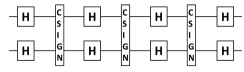
Figure 2: A $2$-qubit gadget for converting an even number of layers of Hadamard gates into an odd number.

For simplicity, suppose that $\left|S\right|=2$, and let $a$ and $b$ be $S$’s elements.  Our gadget, shown in Figure 2, consists of three CSIGN gates (i.e., gates that map $\left|x,y\right\rangle$ to $\left(-1\right)^{xy}\left|x,y\right\rangle$) on $a$ and $b$, sandwiched between Hadamard gates.  Note that we can implement a CSIGN on $a$ and $b$ as $U_{f_{i}}$, where $f_{i}\left(z_{1},\ldots,z_{n}\right):=\left(-1\right)^{z_{a}z_{b}}$.  Meanwhile, the Hadamard gates are just those that are automatically applied between each $U_{f_{i}}$ and $U_{f_{i+1}}$ in a quantum circuit for Forrelation.

To see why the gadget works, consider the following identity:

$$\left(\frac{1}{2}\left(\begin{array}[c]{cccc}1&1&1&1\\ 1&-1&1&-1\\ 1&1&-1&-1\\ 1&-1&-1&1\end{array}\right)\left(\begin{array}[c]{cccc}1&0&0&0\\ 0&1&0&0\\ 0&0&1&0\\ 0&0&0&-1\end{array}\right)\right)^{3}=\left(\begin{array}[c]{cccc}1&0&0&0\\ 0&0&1&0\\ 0&1&0&0\\ 0&0&0&1\end{array}\right).$$

In particular, if we let $\operatorname*{C}$ stand for CSIGN, $\operatorname*{H}^{\otimes 2}$ for Hadamards on two qubits, and $\operatorname*{S}$ for the $2$-qubit SWAP gate, then

$$\operatorname*{H}\nolimits^{\otimes 2}\operatorname*{C}\operatorname*{H}\nolimits^{\otimes 2}\operatorname*{C}\operatorname*{H}\nolimits^{\otimes 2}\operatorname*{C}\operatorname*{H}\nolimits^{\otimes 2}=\operatorname*{S}\operatorname*{H}\nolimits^{\otimes 2}.$$

Contrast this with what happens if we apply the $2$-qubit identity, $\operatorname*{I}$, rather than $\operatorname*{C}$, in the inner layers:

$$\operatorname*{H}\nolimits^{\otimes 2}\operatorname*{I}\operatorname*{H}\nolimits^{\otimes 2}\operatorname*{I}\operatorname*{H}\nolimits^{\otimes 2}\operatorname*{I}\operatorname*{H}\nolimits^{\otimes 2}=\operatorname*{I}.$$

Thus, Hadamards get applied if $\operatorname*{C}$ is chosen for the inner layers, but not if $\operatorname*{I}$ is chosen.  So this gadget has the effect of Hadamarding $a$ and $b$, while not Hadamarding the other qubits in the circuit.  Now, the gadget also has the unintended side effect of swapping $a$ and $b$.  But since we know this is going to happen, we can keep track of it by simply swapping the labels of $a$ and $b$ whenever the gadget is applied.

To generalize to arbitrary subsets $S\subset\left[n\right]$: if $\left|S\right|>2$ is even, then we simply partition $S$ into pairs, and apply the $2$-qubit Hadamard gadget once in succession to each pair.  If $\left|S\right|$ is odd, then the odd qubit in $S$ can be paired with a “dummy qubit,” which is introduced into the circuit for this sole purpose.

Notice that each CSIGN gate is simulated by a single $f_{i}$, while each pair of Hadamards is simulated by three $f_{i}$’s together with the Hadamards that sandwich them.  Thus, we can place a pair of Hadamards after a CSIGN gate, or vice versa, with no difficulty.  To place one CSIGN gate after another, or one pair of Hadamards after another, we insert an $f_{i}=1$ (i.e., a constant $1$ function) in between them, in order to cancel the unwanted Hadamards.

Given a quantum circuit $Q$ on $n$ qubits, consisting of $m$ Hadamard and CCSIGN gates, the end result of our reduction will be a list of Boolean functions $f_{1},\ldots,f_{k}:\left\{0,1\right\}^{n+1}\rightarrow\left\{-1,1\right\}$, with $k=O\left(m\right)$, such that $\Phi_{f_{1},\ldots,f_{k}}=A_{Q}$.  (The $n+1$ comes from the addition of the dummy qubit.)  Furthermore, each $f_{i}\left(z_{1},\ldots,z_{n}\right)$ in the list will have the form $1$ or $\left(-1\right)^{z_{a}z_{b}}$ or $\left(-1\right)^{z_{a}z_{b}z_{c}}$, so will be easy to specify using a Boolean circuit.   

As a side note, suppose we required the functions $f_{1},\ldots,f_{k}$ to depend on at most $2$ input bits, rather than $3$ bits.  In that case, we claim that $k$-fold Forrelation would be in $\mathsf{P}$.  The reason is just that in this case, our quantum circuit for Forrelation would be a stabilizer circuit, so the Gottesman-Knill Theorem would apply.

Examining the proof of Theorem 25, we can derive a stronger consequence.  Define a depth-$d$ quantum circuit as one where the gates are organized into $d$ sequential layers, with the gates within each layer all commuting with one another.  Now, given a depth-$d$ quantum circuit $Q$ over the basis $\left\{\operatorname*{H},\operatorname*{CCSIGN}\right\}$, let QSim_d be the problem of deciding whether $A_{Q}:=\left\langle 0\right|^{\otimes n}Q\left|0\right\rangle^{\otimes n}$ satisfies $A_{Q}\geq\frac{1}{4}$ or $\left|A_{Q}\right|\leq\frac{1}{100}$, promised that one of those is the case.  Then we have the following:

Theorem 26

QSim_d is polynomial-time reducible to explicit $\left(2d+1\right)$-fold Forrelation.  (Moreover, the functions $f_{1},\ldots,f_{2d+1}$ produced by the reduction all have the form $f_{i}\left(x\right)=\left(-1\right)^{p\left(x\right)}$, where $p$ is a degree-$3$ polynomial in the input bits.)

Proof. The only change we need to make to the proof of Theorem 25 is to be a bit more frugal with $f_{i}$’s—using at most two $f_{i}$’s for each layer of $Q$, rather than separate $f_{i}$’s for each gate.

In more detail, a given layer $L$ of $Q$ consists of Hadamard gates on some subset of qubits $S\subseteq\left[n\right]$, as well as CCSIGN gates (which might overlap each other) on some other subset of qubits $T\subseteq\left[n\right]$ satisfying $S\cap T=\varnothing$.  Suppose we want to simulate $L$ using the three functions $f_{i},f_{i+1},f_{i+2}$, together with the Hadamards that sandwich them.  Then we build up the functions as follows: initially $f_{i}=f_{i+1}=f_{i+2}=1$.  For each CCSIGN gate, acting on qubits $a,b,c\in T$, we multiply $f_{i+1}$ by $\left(-1\right)^{z_{a}z_{b}z_{c}}$, leaving $f_{i}$ and $f_{i+2}$ unchanged.  For each pair of Hadamard gates, acting on qubits $a,b\in S$, we multiply $f_{i}$, $f_{i+1}$, and $f_{i+2}$ by $\left(-1\right)^{z_{a}z_{b}}$.  One can check that the end result is

$$\operatorname*{H}\nolimits^{\otimes n}U_{f_{i+2}}\operatorname*{H}\nolimits^{\otimes n}U_{f_{i+1}}\operatorname*{H}\nolimits^{\otimes n}U_{f_{i}}\operatorname*{H}\nolimits^{\otimes n}=\sigma L,$$

where $\sigma$ represents a SWAP gate applied to each pair $a,b\in S$ (something that, as before, we can easily keep track of).

To separate two successive layers of the circuit, we could simply insert a constant function, $f_{i}=1$.  This would yield a $4d$-fold Forrelation instance, $d$ being the number of layers.  If we want to decrease the number of $f_{i}$’s from $4d$ to $2d+1$, then we can eliminate each constant $f_{i}$, together with the Hadamard layers surrounding it (which simply cancel each other out), and then merge $f_{i-1}$ and $f_{i+1}$ into a single $f_{i}$ by multiplying them: $f_{i}\left(x\right)=f_{i-1}\left(x\right)f_{i+1}\left(x\right)$, or $f_{i}\left(x\right)=\left(-1\right)^{p\left(x\right)+q\left(x\right)}$ if $f_{i-1}\left(x\right)=\left(-1\right)^{p\left(x\right)}$ and $f_{i+1}\left(x\right)=\left(-1\right)^{q\left(x\right)}$.

Note that, at the end, each $f_{i}$ is a degree-$3$ polynomial in its input bits, and we again have $\Phi_{f_{1},\ldots,f_{k}}=A_{Q}$.   

So for example, we find that explicit $\log n$-fold Forrelation is a complete promise problem for $\mathsf{P{}romiseBQNC}^{1}$: the class of problems that captures what can be done using log-depth quantum circuits (and which already contains Factoring, by a result of Cleve and Watrous [13]).

7 Appendix: Separations for Sampling and Relation Problems

Let Fourier Sampling be the following problem.  Given oracle access to a Boolean function $f:\left\{0,1\right\}^{n}\rightarrow\left\{-1,1\right\}$, the task is to sample from a distribution D over $\left\{0,1\right\}^{n}$ such that $\left\|\emph{D}-\emph{D}_{f}\right\|\leq\varepsilon$, where $\emph{D}_{f}$ is the distribution defined by

$$\Pr_{\emph{D}_{f}}\left[y\right]=\hat{f}\left(y\right)^{2}=\left(\frac{1}{2^{n}}\sum_{x\in\left\{0,1\right\}^{n}}f\left(x\right)\left(-1\right)^{x\cdot y}\right)^{2}.$$

It is clear that Fourier Sampling is solvable—indeed, with $\varepsilon=0$—by a quantum algorithm that makes just a single query to $f$.  The algorithm consists of a round of Hadamard gates, then a query to $f$, then another round of Hadamard gates, then a measurement in the computational basis.

By contrast, we show in this appendix that any classical randomized algorithm for Fourier Sampling requires $\Omega\left(N/\log N\right)$ queries, where $N=2^{n}$ is the size of $f$’s truth table.  In other words, a much larger quantum versus classical separation can be achieved for sampling problems than for decision problems.

Theorem 27

Fix (say) $\varepsilon=0.01$.  Then the randomized query complexity of Fourier Sampling is $\Omega\left(N/\log N\right)$.

Proof. Let $A$ be a classical algorithm, and let $\mathcal{E}_{f}=\left\{p_{f,y}\right\}_{y\in\left\{0,1\right\}^{n}}$ be the probability distribution output by $A$ when given $f$ as an oracle.  The success condition is that, for all $f$,

$$\frac{1}{2}\sum_{y\in\left\{0,1\right\}^{n}}\left|p_{f,y}-\hat{f}\left(y\right)^{2}\right|\leq\varepsilon.$$

By an averaging argument, this implies that there exists a $y^{\ast}\in\left\{0,1\right\}^{n}$ such that

$$\operatorname*{E}_{f}\left[\left|p_{f,y^{\ast}}-\hat{f}\left(y^{\ast}\right)^{2}\right|\right]\leq\frac{2\varepsilon}{N}.$$

So by Markov’s inequality,

$$\left|p_{f,y^{\ast}}-\hat{f}\left(y^{\ast}\right)^{2}\right|\leq\frac{20\varepsilon}{N}$$

for at least a $9/10$ fraction of $f$’s.  Now assume by symmetry, and without loss of generality, that $y^{\ast}=0^{n}$.  Let $z_{i}:=\frac{1+f\left(x_{i}\right)}{2}$ (where $x_{1},\ldots,x_{N}$ is a lexicographic ordering of inputs), let $Z:=\left(z_{1},\ldots,z_{N}\right)$, and let

$$\left|Z\right|:=z_{1}+\cdots+z_{N}.$$

Then $\hat{f}\left(0^{n}\right)=\left(2\left|Z\right|-N\right)/N$.  The question before us is how many $z_{i}$’s the algorithm $A$ needs to query, in order to output $0^{n}$ (or, as we’ll say, “accept”) with a probability $p_{Z}:=p_{f,0^{n}}$ that satisfies

$$\left|p_{Z}-\left(\frac{2\left|Z\right|}{N}-1\right)^{2}\right|\leq\frac{20\varepsilon}{N}$$ (8)

with probability at least $9/10$ over $Z\in\left\{0,1\right\}^{N}$.

Observe that, without loss of generality, $A$ just nonadaptively queries $t$ randomly-chosen inputs $z_{i_{1}},\ldots,z_{i_{t}}$, and then accepts with a probability $q_{k}$ that depends solely on $k:=z_{i_{1}}+\cdots+z_{i_{t}}$.  For, if $A$ did anything other than this, then by averaging over all $N!$ possible permutations of $Z$, we would obtain an algorithm of this restricted form that made the same number of queries and that was just as likely to satisfy (8).  In particular, this means that the probability $p_{\left|Z\right|}=p_{Z}$ that $A$ accepts $Z$ depends only on $\left|Z\right|$.  Explicitly,

$$p_{w}=\sum_{k=0}^{t}q_{k}r_{k,w},$$ (9)

where

$$r_{k,w}=\frac{1}{2^{N}}\binom{t}{k}\binom{N-t}{w-k}$$

is the probability that $z_{i_{1}}+\cdots+z_{i_{t}}=k$ conditioned on $\left|Z\right|=w$.

Let

$$U :=\left\{Z:\left|\left|Z\right|-\frac{N}{2}\right|\leq\frac{\sqrt{N}}{4}\right\},$$

$$V :=\left\{Z:\left|\left|Z\right|-\frac{N}{2}\right|\in\left[\frac{\sqrt{N}}{2},2\sqrt{N}\right]\right\}.$$

Then note that for sufficiently large $N$,

$$\Pr_{Z}\left[Z\in U\right] \geq\operatorname{erf}\left(\frac{1}{2\sqrt{2}}\right)-o\left(1\right)>0.38,$$

$$\Pr_{Z}\left[Z\in V\right] \geq\operatorname{erf}\left(2\sqrt{2}\right)-\operatorname{erf}\left(\frac{1}{\sqrt{2}}\right)-o\left(1\right)>0.31.$$

This implies that, conditioned on $Z\in U$, we must have

$$p_{Z} \leq\left(\frac{2\left|Z\right|}{N}-1\right)^{2}+\frac{20\varepsilon}{N}$$

$$\leq\left(\frac{2\sqrt{N}/4}{N}\right)^{2}+\frac{20\varepsilon}{N}$$

$$=\frac{0.25+20\varepsilon}{N}$$

$$=\frac{0.45}{N}$$

with probability at least $1-\frac{0.1}{0.38}>2/3$ over $Z$.  Likewise, conditioned on $Z\in V$, we must have

$$p_{Z} \geq\left(\frac{2\left|Z\right|}{N}-1\right)^{2}-\frac{20\varepsilon}{N}$$

$$\geq\frac{1-20\varepsilon}{N}$$

$$=\frac{0.8}{N}$$

with probability at least $1-\frac{0.1}{0.31}>2/3$ over $Z$.

Thus, it suffices to prove a lower bound for the following restricted problem: for at least $2/3$ of strings $Z\in U$, accept with some probability $p_{Z}\leq 0.45/N$, while for at least $2/3$ of strings $Z\in V$, accept with some probability $p_{Z}\geq 0.8/N$.  Indeed, let us assume without loss of generality that if $Z$ is drawn from $U$ then $\left|Z\right|=N/2$ exactly, while if $Z$ is drawn from $V$ then $\left|Z\right|=N/2+2\sqrt{N}$ exactly.  This can only make the distinguishing task easier, and therefore the lower bound stronger.  Note that, because $p_{\left|Z\right|}=p_{Z}$ depends only on $\left|Z\right|$, any algorithm that achieves $p_{Z}\leq 0.45/N$ for at least a $2/3$ fraction of $\left|Z\right|=N/2$ actually achieves that for all $\left|Z\right|=N/2$, while any algorithm that achieves $p_{Z}\geq 0.8/N$ for at least a $2/3$ fraction of $\left|Z\right|=N/2+2\sqrt{N}$ achieves that for all $\left|Z\right|=N/2+2\sqrt{N}$.

Recall from (9) that $p_{\left|Z\right|}=p_{Z}$ is a linear combination of $r_{k,\left|Z\right|}$’s, which are the probabilities for various numbers $k$ of ‘1’ bits to be observed among the $t$ bits queried, conditioned on $\left|Z\right|$ having the value that it does.  Moreover, the coefficients $q_{k}$ in this linear combination are all in $\left[0,1\right]$.  We want to show that, if $t=o\left(N/\log N\right)$, then either $p_{N/2+2\sqrt{N}}=o\left(1/N\right)$ or else $p_{N/2+2\sqrt{N}}-p_{N/2}=o\left(1/N\right)$—either of which suffices to show $A$’s failure.

We deduce this from two probabilistic claims.  First, by a Chernoff bound,

$$\sum_{k=t/2+c\sqrt{t}}^{t}r_{k,N/2+2\sqrt{N}} =\Pr\left[z_{i_{1}}+\cdots+z_{i_{t}}\geq\frac{t}{2}+c\sqrt{t}:\left|Z\right|=\frac{N}{2}+2\sqrt{N}\right]$$

$$\leq\exp\left\{-\frac{1}{3}\frac{\left(\frac{t}{2}+c\sqrt{t}-\left(\frac{t}{2}+\frac{2t}{\sqrt{N}}\right)\right)^{2}}{\frac{t}{2}+\frac{2t}{\sqrt{N}}}\right\}$$

$$\leq\exp\left\{-\frac{1}{3t}\left(c^{2}t-\frac{4ct^{3/2}}{\sqrt{N}}+\frac{4t^{2}}{N}\right)\right\}$$

$$\leq\exp\left\{-\frac{c^{2}}{3}+\frac{4c}{3}\sqrt{\frac{t}{N}}\right\}$$

$$\leq\exp\left\{-\Omega\left(c^{2}\right)\right\}$$

for large $c$.  So in particular, if $c=\omega(\sqrt{\log N})$, then all the events involving observing $k$ ‘1’ bits, for $k\geq t/2+c\sqrt{t}$, have total probability $o\left(1/N\right)$.  This means that, if $A$ worked, then we could set $q_{k}=0$ for all $k\geq t/2+c\sqrt{t}$ without affecting $A$’s success: we would still have $p_{N/2+2\sqrt{N}}-p_{N/2}=\Omega\left(1/N\right)$ and $p_{N/2}=O(1/N)$.

Thus, let us concentrate next on $r_{k,N/2+2\sqrt{N}}$ and $r_{k,N/2}$ for $k\leq t/2+O(\sqrt{t\log N})$.  Here, we look at their ratio:

$$\frac{r_{k,N/2+2\sqrt{N}}}{r_{k,N/2}} =\frac{\binom{N-t}{N/2+2\sqrt{N}-k}}{\binom{N-t}{N/2-k}}$$

$$=\frac{\left(N/2-t+k-2\sqrt{N}+1\right)\cdots\left(N/2-t+k\right)}{\left(N/2-k+1\right)\cdots\left(N/2-k+2\sqrt{N}\right)}$$

$$\leq\left(1+\frac{2k-t-2\sqrt{N}}{N/2-k+1}\right)^{2\sqrt{N}}$$

$$\leq\left(1+\frac{2k-t}{N/4}\right)^{2\sqrt{N}}$$

$$\leq\left(1+O\left(\frac{\sqrt{t\log N}}{N}\right)\right)^{2\sqrt{N}}$$

$$=\exp\left\{O\left(\sqrt{\frac{t\log N}{N}}\right)\right\}.$$

Notice that, if $t=o\left(N/\log N\right)$, then the above ratio is $1+o\left(1\right)$.  This means that taking a nonnegative linear combination of $r_{k,\left|Z\right|}$’s cannot possibly suffice to achieve $p_{N/2}=O(1/N)$ and $p_{N/2+2\sqrt{N}}-p_{N/2}=\Omega\left(1/N\right)$ at the same time.   

We conjecture that Theorem 27 is tight: that is, that there exists a randomized algorithm for Fourier Sampling making $O\left(N/\log N\right)$ queries.  More generally, we conjecture that any approximate sampling problem solvable with $1$ quantum query is also solvable with $O\left(N/\log N\right)$ classical randomized queries.  Still more generally, we conjecture that any approximate sampling problem solvable with $k=O\left(1\right)$ quantum queries is also solvable with $O(N/\left(\log N\right)^{1/k})$ classical randomized queries; and that this is tight, being achieved by a $k$-fold generalization of Fourier Sampling.  In the $k$-fold generalization, we are given oracle access to $k$ Boolean functions $f_{1},\ldots,f_{k}:\left\{0,1\right\}^{n}\rightarrow\left\{-1,1\right\}$.  The task is to sample from a distribution D over $\left\{0,1\right\}^{n}$ such that $\left\|\emph{D}-\emph{D}_{f_{1},\ldots,f_{k}}\right\|\leq\varepsilon$, where $\emph{D}_{f_{1},\ldots,f_{k}}$ is the distribution defined by

$$\Pr_{\emph{D}_{f_{1},\ldots,f_{k}}}\left[y\right]=\left(\frac{1}{2^{n\left(k+1\right)/2}}\sum_{x_{1},\ldots,x_{k}\in\left\{0,1\right\}^{n}}f_{1}\left(x_{1}\right)\left(-1\right)^{x_{1}\cdot x_{2}}f_{2}\left(x_{2}\right)\left(-1\right)^{x_{2}\cdot x_{3}}\cdots f_{k}\left(x_{k}\right)\left(-1\right)^{x_{k}\cdot y}\right)^{2}.$$

So far, we have discussed separations for approximate sampling problems.  But it is also possible to modify Fourier Sampling to produce a relation problem—that is, a problem of outputting any element of a set $S$ of “valid solutions”—with a large quantum/classical separation.  One way to do this would be to use the construction of Aaronson [2], which, given any approximate sampling problem, uses Kolmogorov complexity to produce a relation problem of roughly equivalent difficulty.  Unfortunately, that construction will blow up the quantum query complexity from $1$ to $O\left(\log N\right)$, weakening the result.  A more direct approach would be to consider the following relation problem: given oracle access to a Boolean function $f:\left\{0,1\right\}^{n}\rightarrow\left\{-1,1\right\}$, output any string $y\in\left\{0,1\right\}^{n}$ such that $\left|\hat{f}\left(y\right)\right|\geq c$.  If we use the obvious Fourier sampling algorithm, this problem is solvable with $1$ quantum query, with success probability asymptotically equal to

$$\frac{2}{\sqrt{2\pi}}\int_{c}^{\infty}e^{-x^{2}/2}x^{2}dx.$$

On the other hand, it is a plausible conjecture that any classical randomized algorithm that makes $o\left(N/\log N\right)$ queries to $f$, can solve the relation problem with probability at most about

$$\frac{2}{\sqrt{2\pi}}\int_{c}^{\infty}e^{-x^{2}/2}dx.$$

If (say) $c=1$, this would give us an $0.8$ versus $0.317$ gap in success probabilities.  That gap could be boosted further using amplification (which, however, would increase the quantum query complexity, from $1$ to some larger constant).

8 Appendix: Estimator for Arbitrary Bounded Quadratics

Assume that we have an arbitrary degree-$k$ polynomial

$$p\left(x_{1},\ldots,x_{N}\right)=\sum_{I\subseteq\left[N\right]:\left|I\right|\leq k}a_{I}\prod_{i\in I}x_{i},$$

with $p\left(x\right)\in[-1,1]$ whenever $x\in\left\{-1,1\right\}^{N}$.  We would like to show that $p\left(x\right)$ can be estimated by a randomized algorithm that makes $O\left(N^{1-1/k}\right)$ queries, using a sampling procedure similar to what we used in Section 5 for the special case of block-multilinear polynomials.  For our previous proof to work, we need there to exist a sequence of variable-splittings that introduces $O(N)$ new variables, and that transforms $p(x_{1},\ldots,x_{N})$ into a polynomial

$$q(x_{1},\ldots,x_{M})=\sum_{I\subseteq[M]:|I|\leq k}b_{I}\prod_{i\in I}x_{i}$$

that satisfies the following two requirements:

1. $\sum_{I}b_{I}^{2}=O(\frac{1}{N})$;

2. for all $l\in\left[k-1\right]$, we have

   $$\sum_{I,J:,I\neq J,|I\cap J|=l}b_{I}b_{J}=O\left(\frac{1}{N^{l/k}}\right).$$ (10)

Requirement (i) is for the bound on the variance of the “warmup estimator,” in Section 5.3.  Requirement (ii) is for the “real estimator,” in Section 5.4.  Below, we will be able to prove requirement (i) for any $k$, and requirement (ii) in the special case $k=2$.

8.1 Fourier Basics

Given a real polynomial $p:\left\{-1,1\right\}^{N}\rightarrow\mathbb{R}$, we consider the following notions:

$$\operatorname{Var}\left[p\right] :=\operatorname{E}\left[\left(p\left(x\right)-\operatorname{E}\left[p\left(x\right)\right]\right)^{2}\right],$$

$$\operatorname{Inf}_{i}\left[p\right] :=\operatorname{E}\left[\left(p\left(x^{i}\right)-p\left(x\right)\right)^{2}\right],$$

$$\left\|p\right\|_{\infty} :=\max_{x\in\left\{-1,1\right\}^{N}}\left|p\left(x\right)\right|$$

(where $x^{i}$ means $x$ with the $i^{th}$ bit flipped).  Also, let $\hat{p}\left(S\right)$ be the Fourier coefficient corresponding to the subset $S\subseteq\left[N\right]$—or equivalently, the coefficient in $p$ of the monomial $\prod_{i\in S}x_{i}$.

Note that, since $\sum_{I}b_{I}^{2}=\operatorname{Var}[q]$, requirement (i) is equivalent to $\operatorname{Var}[q]=O(\frac{1}{N})$.

From elementary Fourier analysis, we have the following useful lemma.

Lemma 28

If $p:\left\{-1,1\right\}^{N}\rightarrow\mathbb{R}$ is a real polynomial of degree $k$, then

$$\sum_{i\in\left[N\right]}\operatorname{Inf}_{i}\left[p\right]\leq k\operatorname{Var}\left[p\right].$$

Proof. We have

$$\operatorname{Inf}_{i}\left[p\right]=\sum_{S\ni i}\hat{p}\left(S\right)^{2},$$

and hence

$$\sum_{i\in\left[N\right]}\operatorname{Inf}_{i}\left[p\right]=\sum_{\left|S\right|\leq k}\left|S\right|\hat{p}\left(S\right)^{2}\leq k\sum_{\left|S\right|\leq k}\hat{p}\left(S\right)^{2}=k\operatorname{Var}\left[p\right].$$

 

8.2 Requirement (i)

Our goal is to find variables $x_{i}$ in $p$ with large influences (that is, large values of $\operatorname{Inf}_{i}\left[p\right]$).  To do so, we will use the following result of Dinur et al. [14, Theorem 3].

Theorem 29 ([14], Theorem 3)

There exists a constant $C$ for which the following holds.  Suppose $p:\left\{-1,1\right\}^{N}\rightarrow\mathbb{R}$ is a real polynomial of degree $k$, which satisfies $\operatorname{Var}[p]=1$ and $\operatorname{Inf}_{i}\left[p\right]\leq t^{2}C^{-k}$ for all $i\in\left[N\right]$.  Then

$$\Pr_{x\in\left\{-1,1\right\}^{N}}\left[\left|p\left(x\right)\right|\geq t\right]\geq\exp(-Ct^{2}k^{2}\log k).$$

Theorem 29 means, in particular, that if $\operatorname{Var}\left[p\right]=1$ and $\operatorname{Inf}_{i}\left[p\right]\leq t^{-2}C^{-k}$ for all $i\in\left[N\right]$, then $\left\|p\right\|_{\infty}\geq t$: in other words, there exists an $x\in\left\{-1,1\right\}^{N}$ such that $\left|p\left(x\right)\right|\geq t$.  By rescaling, we can turn this into the following.

Corollary 30

There exists a constant $C$ for which the following holds.  Suppose $p:\left\{-1,1\right\}^{N}\rightarrow\mathbb{R}$ is a real polynomial of degree $k$, which satisfies $\left\|p\right\|_{\infty}\leq 1$ and $\operatorname{Var}\left[p\right]\geq\frac{C}{N}$.  Then there exists an $i\in\left[N\right]$ such that $\operatorname{Inf}_{i}\left[p\right]\geq\frac{1}{C^{k}}\operatorname{Var}\left[p\right]^{2}$.

Proof. We can reword Theorem 29 as follows: if $\left\|p\right\|_{\infty}\leq t$ and $\operatorname{Var}\left[p\right]=1$, then there exists an $i\in\left[N\right]$ such that $\operatorname{Inf}_{i}[p]\geq\frac{t^{2}}{C^{k}}$.  Now suppose $\left\|p\right\|_{\infty}\leq 1$.  Then define a new polynomial $q:=\frac{p}{\sqrt{\operatorname{Var}\left[p\right]}}$.  We have $\operatorname{Var}[q]=1$ and $\left\|q\right\|_{\infty}\leq\frac{1}{\sqrt{\operatorname{Var}\left[p\right]}}$, which implies that there exists an $i\in\left[N\right]$ such that $\operatorname{Inf}_{i}\left[q\right]\geq\frac{\operatorname{Var}\left[p\right]}{C^{k}}$, or equivalently $\operatorname{Inf}_{i}\left[p\right]\geq\frac{\operatorname{Var}\left[p\right]^{2}}{C^{k}}$.   

We now consider the following algorithm for variable-splitting.  We start with $p_{0}:=p$.  We then repeat the following, for $j\in\{0,1,2,\ldots\}$:

1. If $\operatorname{Var}\left[p_{j}\right]<\frac{C}{N}$, then halt and output $p_{j}$.

2. Otherwise, choose some variable $x_{i}$ such that $\operatorname{Inf}_{i}\left[p\right]\geq\frac{1}{C^{k}}\operatorname{Var}\left[p\right]^{2}$ (which is guaranteed to exist by Corollary 30).  Let $p_{j+1}$ be the polynomial obtained from $p_{j}$ by splitting $x_{i}$ into two variables.  (In other words, by defining new variables $x_{i,1}$ and $x_{i,2}$, and then replacing every occurrence of $x_{i}$ in $p_{j}$ by $\frac{x_{i,1}+x_{i,2}}{2}$.)

When the algorithm halts (say at step $J$), we must have $\operatorname{Var}\left[p_{J}\right]<\frac{C}{N}$.  Furthermore, observe that for every $j$,

$$\operatorname{Var}[p_{j+1}] =\operatorname{Var}[p_{j}]-\frac{\operatorname{Inf}_{i}\left[p_{j}\right]}{2}$$

$$\leq\operatorname{Var}\left[p_{j}\right]-\frac{\operatorname{Var}\left[p_{j}\right]^{2}}{2C^{k}}.$$

Solving this recurrence (together with the initial condition $\operatorname{Var}\left[p_{0}\right]\leq 1$) implies that the algorithm can continue for at most $O\left(N\right)$ steps until $\operatorname{Var}\left[p_{J}\right]=O(1/N)$.  Therefore, the algorithm introduces at most $O\left(N\right)$ new variables.

8.3 Requirement (ii)

We now show how to satisfy requirement (ii) in the special case $k=2$.  To do so, we will need another result from Dinur et al. [14].

Lemma 31 ([14], Lemma 1.3)

There exists a constant $C$ such that the following holds.  Let $p:\left\{-1,1\right\}^{N}\rightarrow\mathbb{R}$ be a polynomial of degree $k$, and suppose that

$$\sum_{i\in\left[N\right]}\hat{p}\left(\left\{i\right\}\right)^{2}\geq 1$$

whereas $\left|\hat{p}\left(\left\{i\right\}\right)\right|\leq\frac{1}{Ckt}$ for all $i\in\left[N\right]$.  Then

$$\Pr_{x\in\left\{-1,1\right\}^{N}}\left[\left|p\left(x\right)\right|\geq t\right]\geq\exp(-Ct^{2}k^{2}).$$

By rescaling $p$ (similarly to Corollary 30), we can transform Lemma 31 into the following.

Corollary 32

There exists a constant $C$ such that the following holds.  For any bounded real polynomial $p:\{-1,1\}^{N}\rightarrow\left[-1,1\right]$ of degree $k$ that satisfies

$$\sum_{i\in\left[N\right]}\hat{p}\left(\left\{i\right\}\right)^{2}=v,$$

there exists an $i\in\left[N\right]$ such that $\left|\hat{p}\left(\left\{i\right\}\right)\right|\geq\frac{v}{Ck}$.

Proof. Let us define a new polynomial $q\left(x\right):=\frac{p\left(x\right)}{\sqrt{v}}$.  Then $q\left(x\right)\in\left[-\frac{1}{\sqrt{v}},\frac{1}{\sqrt{v}}\right]$ for all $x\in\left\{-1,1\right\}^{N}$, and

$$\sum_{i\in\left[N\right]}\hat{q}\left(\left\{i\right\}\right)^{2}=1.$$

So by Lemma 31, there must exist an index $i\in\left[N\right]$ such that

$$\left|\hat{q}\left(\left\{i\right\}\right)\right|>\frac{\sqrt{v}}{Ck}$$

and hence

$$\left|\hat{p}\left(\left\{i\right\}\right)\right|>\frac{v}{Ck}.$$

 

We now specialize to the case $k=2$.  Observe that, given a bounded quadratic polynomial $p:\left\{-1,1\right\}^{N}\rightarrow\left[-1,1\right]$ that we are trying to estimate, we can assume without loss of generality that $p$ is homogeneous: in other words, is a quadratic form.  First of all, if $p$ contains a degree-$0$ term (i.e., an additive constant) $c$, then we can replace it by the degree-$2$ term $cx_{1}^{2}$.  Next, suppose we decompose $p$ as a sum of its quadratic part $p_{2}$ and its linear part $p_{1}$:

$$p\left(x\right)=p_{2}\left(x\right)+p_{1}\left(x\right).$$

Then

$$p\left(-x\right)=p_{2}\left(x\right)-p_{1}\left(x\right)$$

is also bounded in $\left[-1,1\right]$ for all $x\in\left\{-1,1\right\}^{N}$.  So

$$p_{1}\left(x\right)=\frac{p\left(x\right)-p\left(-x\right)}{2}\in\left[-1,1\right],$$

and likewise $p_{2}\left(x\right)\in\left[-1,1\right]$, for all $x\in\left\{-1,1\right\}^{N}$.  Hence we can simply estimate $p_{2}\left(x\right)$ and $p_{1}\left(x\right)$ separately and then sum them.  Furthermore, $p_{1}$ has the form

$$p_{1}\left(x\right)=a_{1}x_{1}+\cdots+a_{n}x_{n}$$

for some coefficients satisfying $\left|a_{1}\right|+\cdots+\left|a_{n}\right|\leq 1$.  By standard tail bounds, such a linear form is easy to estimate to within $\pm\varepsilon$ by querying only $O\left(1\right)$ variables $x_{i}$.

So our problem reduces to estimating the bounded quadratic form $p_{2}\left(x\right)$.  To do this, the first step is to apply the variable-splitting algorithm described in Section 8.2.  This produces a new bounded quadratic form, which we denote $P$:

$$P(x_{1},\ldots,x_{N})=\sum_{i,j\in\left[N\right]}a_{i,j}x_{i}x_{j}.$$

(Abusing notation, we continue to call the number of variables $N$, even though $O\left(N\right)$ new variables have been introduced.)  We have $\operatorname{Var}[P]=O(\frac{1}{N})$.  Now, our goal is to perform another sequence of variable-splittings, which should introduce $O(N)$ new variables and achieve requirement (ii).

Observe that, to achieve requirement (ii), it suffices to ensure

$$\sum_{i\in\left[N\right]}\left(\sum_{i\neq j}a_{ij}\right)^{2}=O\left(\frac{1}{\sqrt{N}}\right).$$ (11)

For if we achieve (11), then we can obtain the original requirement (ii) by removing all squares $a_{ij}^{2}$ from the left hand side (which only decreases it) and dividing it by $2$.

Let

$$\operatorname{I}_{i}\left[P\right] :=\left(\sum_{i\neq j}a_{ij}\right)^{2},$$

$$\operatorname{V}\left[P\right] :=\sum_{i\in[N]}\operatorname{I}_{i}\left[P\right].$$

We show the following counterpart of Corollary 30.

Lemma 33

There exists a constant $C$ for which the following holds.  If $\operatorname{V}\left[P\right]\geq\frac{C\log N}{N}$, then there exists an $i\in\left[N\right]$ such that $\operatorname{I}_{i}\left[P\right]=\Omega(\operatorname{V}\left[P\right]^{2})$.

Proof. We take $P(x_{1},\ldots,x_{N})$ and, for each $i\in[N]$, substitute $x_{i}=1$ with probability $1/2$ (with choices for different $i$ made independently).  Let $q$ be the resulting polynomial.

The key claim is the following: let $x_{i}$ be a variable for which we do not substitute $x_{i}=1$.  Then

$$\left|\hat{q}\left(\left\{i\right\}\right)-\frac{1}{2}\sum_{i\neq j}a_{ij}\right|=O\left(\sqrt{\operatorname{Inf}_{i}[P]\log\frac{1}{\epsilon}}\right)$$ (12)

with probability at least $1-\epsilon$.

To prove the claim: since each term $x_{i}x_{j}$ is transformed into $x_{i}$ with probability $1/2$ by substituting $x_{i}=1$, the expectation of $\hat{q}\left(\left\{i\right\}\right)$ is equal to $\frac{1}{2}\sum_{j\neq i}a_{ij}$.  Since the decision to substitute or not substitute $x_{i}=1$ changes the value of $\hat{q}\left(\left\{i\right\}\right)$ by the amount $a_{ij}$, Azuma’s inequality implies

$$\Pr\left[\left|\hat{q}\left(\left\{i\right\}\right)-\frac{1}{2}\sum_{i\neq j}a_{ij}\right|\geq t\right]\leq\exp\left(-\frac{t^{2}}{2\sum_{j\in\left[N\right]}a_{ij}^{2}}\right).$$

Using $\operatorname{Inf}_{i}[P]=\sum_{j\in\left[N\right]}a_{ij}^{2}$ and taking $t=\sqrt{2\operatorname{Inf}_{i}[P]\log\frac{1}{\epsilon}}$ completes the proof.

We now show how the claim implies the lemma.  Let $\epsilon=\frac{1}{2N}$.  Then we can make the substitutions so that (12) holds for all $i\in[N]$.  By substituting $\epsilon=\frac{1}{2N}$ into (12), we have

$$\left|\hat{q}\left(\left\{i\right\}\right)\right|\in\left[\frac{\sqrt{\operatorname{I}_{i}\left[P\right]}}{2}-O\left(\sqrt{\operatorname{Inf}_{i}\left[P\right]\log N}\right),\frac{\sqrt{\operatorname{I}_{i}\left[P\right]}}{2}+O\left(\sqrt{\operatorname{Inf}_{i}\left[P\right]\log N}\right)\right]$$ (13)

By squaring (13) and summing over all $i\in\left[N\right]$, we obtain

$$\left|\sum_{i\in\left[N\right]}\hat{q}\left(\left\{i\right\}\right)^{2}-\frac{1}{4}\sum_{i\in\left[N\right]}\operatorname{I}_{i}\left[P\right]\right| =O\left(\sqrt{\log N}\right)\sum_{i\in\left[N\right]}\sqrt{\operatorname{I}_{i}\left[P\right]\operatorname{Inf}_{i}\left[P\right]}+O\left(\log N\right)\sum_{i\in\left[N\right]}\operatorname{Inf}_{i}\left[P\right]$$

$$\leq O\left(\sqrt{\log N}\right)\sqrt{\sum_{i\in\left[N\right]}\operatorname{I}_{i}\left[P\right]\cdot\sum_{i\in\left[N\right]}\operatorname{Inf}_{i}\left[P\right]}+O\left(\log N\right)\sum_{i\in\left[N\right]}\operatorname{Inf}_{i}\left[P\right]$$

$$\leq O\left(\sqrt{\log N}\right)\sqrt{\operatorname{V}\left[P\right]\cdot 2\operatorname{Var}\left[P\right]}+O\left(\log N\right)\cdot 2\operatorname{Var}\left[P\right]$$

$$=O\left(\sqrt{\operatorname{V}\left[P\right]\frac{\log N}{N}}+\frac{\log N}{N}\right),$$

where the second line used Cauchy-Schwarz and the third used Lemma 28.

Now, if $\operatorname{V}\left[P\right]\geq C\frac{\log N}{N}$ for a sufficiently large constant $C$, then the above implies that

$$\sum_{i\in\left[N\right]}\hat{q}\left(\left\{i\right\}\right)^{2} \geq\frac{1}{4}\operatorname{V}\left[P\right]-O\left(\sqrt{\operatorname{V}\left[P\right]\frac{\log N}{N}}+\frac{\log N}{N}\right)$$

$$=\Omega\left(\operatorname{V}\left[P\right]\right).$$

By Corollary 32, this means that there exists an index $i\in\left[N\right]$ such that $\left|\hat{q}\left(\left\{i\right\}\right)\right|=\Omega(\operatorname{V}\left[P\right])$.  From equation (13), we get that $\sqrt{\operatorname{I}_{i}\left[P\right]}=\Omega(\operatorname{V}\left[P\right])$ and $\operatorname{I}_{i}\left[P\right]=\Omega(\operatorname{V}\left[P\right]^{2})$.   

Given Lemma 33, we can use the same algorithm as in the previous section.  That is, we repeatedly choose a variable $i\in\left[N\right]$ that maximizes $\operatorname{I}_{i}\left[P\right]$ and split the variable $x_{i}$.  Let $p_{0},p_{1},\ldots$ be the resulting sequence of polynomials.  Initially, we have

$$\operatorname{V}\left[p_{0}\right]=\sum_{i}\left(\sum_{j\neq i}a_{ij}\right)^{2}\leq N\sum_{i}\sum_{j}a_{ij}^{2}=O(1),$$

with the last equality following from $\operatorname{Var}[P]=O(\frac{1}{N})$, which was achieved by the previous sequence of variable-splittings.  We also have

$$\operatorname{V}[p_{j+1}]\leq\operatorname{V}[p_{j}]-\Omega(\operatorname{V}[p_{j}]^{2}),$$

as long as $\operatorname{V}[p_{j}]\geq\frac{C\log N}{N}$.  This means that after $O(N/\log N)$ variable-splittings, we achieve $\operatorname{V}[p_{j}]<\frac{C\log N}{N}$, which is substantially stronger than the requirement (11) that we needed.

9 Appendix: Lower Bound for $k$-fold Forrelation

In this appendix, we use the machinery developed in Section 4 to prove a $\widetilde{\Omega}(\sqrt{N})$ lower bound on the randomized query complexity of $k$-fold Forrelation, for all $k\geq 2$.  Ideally, of course, we would like to prove a lower bound that gets better as $k$ gets larger, but even proving the same kind of lower bound that we had in the $k=2$ case will take some work.

In $k$-fold Forrelation, recall that we are given oracle access to Boolean functions $f_{1},\ldots,f_{k}:\left\{0,1\right\}^{n}\rightarrow\left\{-1,1\right\}$, and are interested in the quantity

$$\Phi_{f_{1},\ldots,f_{k}}:=\frac{1}{2^{\left(k+1\right)n/2}}\sum_{x_{1},\ldots,x_{k}\in\left\{0,1\right\}^{n}}f_{1}\left(x_{1}\right)\left(-1\right)^{x_{1}\cdot x_{2}}f_{2}\left(x_{2}\right)\left(-1\right)^{x_{2}\cdot x_{3}}\cdots\left(-1\right)^{x_{k-1}\cdot x_{k}}f_{k}\left(x_{k}\right).$$

The problem is to decide whether $\left|\Phi_{f_{1},\ldots,f_{k}}\right|\leq\frac{1}{100}$ or $\Phi_{f_{1},\ldots,f_{k}}\geq\frac{3}{5}$, promised that one of these is the case.

We will prove a lower bound for $k$-fold Forrelation by reducing the Gaussian Distinguishing problem to it, and then applying Theorem 11—thereby illustrating the usefulness of formulating a general lower bound for Gaussian Distinguishing.

9.1 Concentration Inequalities

The first step is to prove some concentration inequalities for $k$-fold Forrelation.  In what follows, recall that $f_{\ell}^{\left(x\right)}\left(x_{\ell}\right)$ is defined as $f_{\ell}\left(x_{\ell}\right)\left(-1\right)^{x_{\ell}\cdot x}$, for all $\ell\in\left[k\right]$ and $x_{\ell},x\in\left\{0,1\right\}^{n}$.

Lemma 34

Suppose $f_{1},\ldots,f_{k}:\left\{0,1\right\}^{n}\rightarrow\left\{-1,1\right\}$ are chosen uniformly at random.  Then

$$\Pr_{f_{1},\ldots,f_{k}}\left[\left|\Phi_{f_{1},\ldots,f_{k}}\right|\geq\frac{t}{\sqrt{N}}\right]=O\left(\frac{1}{t^{t}}\right).$$

Proof. Imagine that $f_{1},\ldots,f_{k-1}$ are fixed, so that we are considering $\Phi_{f_{1},\ldots,f_{k}}$ solely as a function of $f_{k}$.  We have

$$\Phi_{f_{1},\ldots,f_{k}}=\frac{1}{\sqrt{N}}\sum_{x\in\left\{0,1\right\}^{n}}\alpha_{x}f_{k}\left(x\right)$$

where

$$\alpha_{x}=\Phi_{f_{1},\ldots,f_{k-2},f_{k-1}^{\left(x\right)}}=\frac{1}{2^{kn/2}}\sum_{x_{1},\ldots,x_{k-1}\in\left\{0,1\right\}^{n}}f_{1}\left(x_{1}\right)\left(-1\right)^{x_{1}\cdot x_{2}}\cdots\left(-1\right)^{x_{k-2}\cdot x_{k-1}}f_{k-1}\left(x_{k-1}\right)\left(-1\right)^{x_{k-1}\cdot x}.$$

Thus, by equation (1),

$$\sum_{x\in\left\{0,1\right\}^{n}}\alpha_{x}^{2}=\sum_{x\in\left\{0,1\right\}^{n}}\Phi_{f_{1},\ldots,f_{k-2},f_{k-1}^{\left(x\right)}}^{2}=1.$$

So in particular, $\left|\alpha_{x}\right|\leq 1$ for all $x$.  We now appeal to Bennett’s inequality, which tells us that

$$\Pr_{f_{k}:\left\{0,1\right\}^{n}\rightarrow\left\{-1,1\right\}}\left[\left|\sum_{x\in\left\{0,1\right\}^{n}}\alpha_{x}f_{k}\left(x\right)\right|\geq t\right]\leq 2\exp\left(-h\left(t\right)\right)$$

where

$$h\left(t\right):=\left(1+t\right)\ln\left(1+t\right)-t.$$

 

The following is also useful.

Lemma 35

Suppose $f_{1},\ldots,f_{k}:\left\{0,1\right\}^{n}\rightarrow\left\{-1,1\right\}$ are chosen uniformly at random.  Then with probability $1-O\left(1/N\right)$, we have

$$\left|\sum_{z~{}:~{}z\cdot y=0}\Phi_{f_{1},\ldots,f_{k-1},f_{k}^{\left(z\right)}}^{2}-\frac{1}{2}\right|\leq\frac{\log^{5/2}N}{\sqrt{N}}$$

for all $y\in\left\{0,1\right\}^{n}$.

Proof. By symmetry, we can assume without loss of generality that $y=10\cdots 0$, so that the sum is over all $z$ that start with $0$.

As in the proof of Lemma 34, imagine that $f_{1},\ldots,f_{k-1}$ are fixed, so that we are considering

$$\Phi_{f_{1},\ldots,f_{k-1},f_{k}^{\left(z\right)}}=\frac{1}{\sqrt{N}}\sum_{x\in\left\{0,1\right\}^{n}}\alpha_{x}f_{k}\left(x\right)\left(-1\right)^{x\cdot z}$$

solely as a function of $f_{k}$.  Then it is not hard to see that

$$\sum_{z~{}:~{}z\cdot y=0}\Phi_{f_{1},\ldots,f_{k-1},f_{k}^{\left(z\right)}}^{2}$$

is just the probability of measuring an output string that starts with $0$ when the Forrelation algorithm is run on $f_{1},\ldots,f_{k}$, which also equals

$$\sum_{x\in\left\{0,1\right\}^{n-1}}\left(\frac{\alpha_{0x}f_{k}\left(0x\right)+\alpha_{1x}f_{k}\left(1x\right)}{\sqrt{2}}\right)^{2} =\frac{1}{2}\sum_{x\in\left\{0,1\right\}^{n-1}}\left(\alpha_{0x}f_{k}\left(0x\right)+\alpha_{1x}f_{k}\left(1x\right)\right)^{2}$$

$$=\frac{1}{2}\sum_{x\in\left\{0,1\right\}^{n-1}}\left(\alpha_{0x}^{2}+\alpha_{1x}^{2}+2\alpha_{0x}\alpha_{1x}f_{k}\left(0x\right)f_{k}\left(1x\right)\right)$$

$$=\frac{1}{2}+\sum_{x\in\left\{0,1\right\}^{n-1}}\alpha_{0x}\alpha_{1x}f_{k}\left(0x\right)f_{k}\left(1x\right).$$

Now, each $f_{k}\left(0x\right)f_{k}\left(1x\right)$ is an independent, uniform $\left\{-1,1\right\}$ random variable.  Furthermore, by Lemma 34, with $1-o\left(1/N\right)$ probability we have $\left|\alpha_{x}\right|\leq\frac{\log N}{\sqrt{N}}$ for all $x\in\left\{0,1\right\}^{n}$, in which case

$$\left|\alpha_{0x}\alpha_{1x}\right|\leq\frac{\log^{2}N}{N}$$

for all $x\in\left\{0,1\right\}^{n-1}$.  By Hoeffding’s inequality, it follows that

$$\Pr\left[\left|\sum_{z~{}:~{}z\cdot y=0}\Phi_{f_{1},\ldots,f_{k-1},f_{k}^{\left(z\right)}}^{2}-\frac{1}{2}\right|\geq\frac{t}{\sqrt{N}}\right] \leq 2\exp\left(-\frac{2(t/\sqrt{N})^{2}}{\left(N/2\right)\left(\frac{2\log^{2}N}{N}\right)^{2}}\right)$$

$$=2\exp\left(-\frac{t^{2}}{4\log^{4}N}\right).$$

Setting $t=C\log^{5/2}N$ for some constant $C$, this probability is at most $1/N^{2}$.  So by the union bound, the probability is at most $1/N$ when summed over all $y$.   

9.2 Continuous/Discrete Hybrid

Just like we did in the $k=2$ case, it is convenient to define a continuous analogue of the $k$-fold Forrelation problem—though in this case, the problem will be a hybrid of continuous and discrete.  In $k$-fold Real Forrelation, we are given oracle access to functions $f_{1},\ldots,f_{k-2}:\left\{0,1\right\}^{n}\rightarrow\left\{-1,1\right\}$ as well as $f_{k-1},f_{k}:\left\{0,1\right\}^{n}\rightarrow\mathbb{R}$.  We are promised that each $f_{i}\left(x_{i}\right)$ (for $i\in\left[k-2\right]$) is chosen uniformly and independently from $\left\{-1,1\right\}$, and also that one of the following holds:

1. Uniform measure $\mathcal{U}$: Each $f_{k-1}\left(x_{k-1}\right)$ and $f_{k}\left(x_{k}\right)$ is an independent $\mathcal{N}\left(0,1\right)$ Gaussian.

2. Forrelated measure $\mathcal{F}$: Each $f_{k-1}\left(x_{k-1}\right)$ is an independent $\mathcal{N}\left(0,1\right)$ Gaussian, and each $f_{k}\left(x_{k}\right)$ is set equal to

   $$\frac{1}{2^{\left(k-1\right)n/2}}\sum_{x_{1},\ldots,x_{k-1}\in\left\{0,1\right\}^{n}}f_{1}\left(x_{1}\right)\left(-1\right)^{x_{1}\cdot x_{2}}\cdots\left(-1\right)^{x_{k-2}\cdot x_{k-1}}f_{k-1}\left(x_{k-1}\right)\left(-1\right)^{x_{k-1}\cdot x_{k}}.$$

The problem is to decide whether (i) or (ii) holds.

Here is another way to think about $k$-fold Real Forrelation: let

$$f\left(x_{k-1}\right):=c_{x_{k-1}}f_{k-1}\left(x_{k-1}\right),~{}~{}~{}~{}~{}~{}~{}~{}~{}~{}g\left(x_{k}\right):=f_{k}\left(x_{k}\right),$$

where

$$c_{x_{k-1}} =\sqrt{N}\Phi_{f_{1},\ldots,f_{k-3},f_{k-2}^{\left(x_{k-1}\right)}}$$

$$=\frac{1}{2^{\left(k-2\right)n/2}}\sum_{x_{1},\ldots,x_{k-2}\in\left\{0,1\right\}^{n}}f_{1}\left(x_{1}\right)\left(-1\right)^{x_{1}\cdot x_{2}}\cdots f_{1}\left(x_{k-2}\right)\left(-1\right)^{x_{k-2}\cdot x_{k-1}}.$$

Then

$$\Phi_{f_{1},\ldots,f_{k}}=\Phi_{f,g}=\frac{1}{2^{3n/2}}\sum_{x,y\in\left\{0,1\right\}^{n}}f\left(x\right)\left(-1\right)^{x\cdot y}g\left(y\right).$$

In other words, we can think of $k$-fold Real Forrelation as equivalent to ordinary, $2$-fold Real Forrelation on the functions $f_{k-1}\left(x\right)$ and $f_{k}\left(y\right)$, except that each $f_{k-1}\left(x\right)$ is “twisted” by a multiplicative factor $c_{x}$ depending on $f_{1},\ldots,f_{k-2}$.  We have the following useful fact.

Proposition 36

With $1-o\left(1/N\right)$ probability over $f_{1},\ldots,f_{k-2}$, we have $\left|c_{x}\right|\leq\log N$ for all $x\in\left\{0,1\right\}^{n}$.

Proof. By Lemma 34,

$$\Pr_{f_{1},\ldots,f_{k-2}}\left[\left|c_{x}\right|\geq\log N\right]=O\left(\frac{1}{\left(\log N\right)^{\log N}}\right)=o\left(\frac{1}{N^{2}}\right).$$

The proposition now follows from the union bound.   

Note also that

$$\sum_{x\in\left\{0,1\right\}^{n}}c_{x}^{2}=N.$$

Next, we prove a $k$-fold analogue of Theorem 9, showing that $k$-fold Real Forrelation can be reduced to Boolean $k$-fold Forrelation.

Theorem 37

Fix $f_{1},\ldots,f_{k-2}$ (or equivalently, the multipliers $c_{x}$).  Suppose $\left\langle f,g\right\rangle=\left\langle f_{k-1},f_{k}\right\rangle$ are drawn from the forrelated measure $\mathcal{F}$.  Define Boolean functions $F,G:\left\{0,1\right\}^{n}\rightarrow\left\{-1,1\right\}$ by $F\left(x\right):=\operatorname*{sgn}\left(f\left(x\right)\right)$ and $G\left(y\right):=\operatorname*{sgn}\left(g\left(y\right)\right)$.  Then

$$\operatorname{E}\left[\Phi_{F,G}\right]=\frac{2}{\pi}\pm O\left(\frac{\log^{3}N}{N}\right).$$

Proof. By Proposition 36, we can assume without loss of generality that $\left|c_{x}\right|\leq\log N$ for all $x\in\left\{0,1\right\}^{n}$ (the times when this assumption fails can only change $\operatorname{E}\left[\Phi_{F,G}\right]$ by $o\left(1/N\right)$).

By linearity of expectation, it suffices to calculate $\operatorname{E}\left[c_{x}F\left(x\right)\left(-1\right)^{x\cdot y}G\left(y\right)\right]$ for some specific $x,y$ pair.  Let $v\in\mathbb{R}^{N}$ be a vector of independent $\mathcal{N}\left(0,1\right)$ Gaussians.  Then we can consider $\left\langle F,G\right\rangle$ to have been generated as follows:

$$F\left(x\right) =\operatorname*{sgn}\left(v_{x}\right),$$

$$G\left(y\right) =\operatorname*{sgn}\left(\sum_{x\in\left\{0,1\right\}^{n}}c_{x}v_{x}\left(-1\right)^{x\cdot y}\right).$$

Let

$$Z:=\sum_{x^{\prime}\neq x}c_{x^{\prime}}v_{x^{\prime}}\left(-1\right)^{x^{\prime}\cdot y},$$

and let $G^{\prime}\left(y\right):=\operatorname*{sgn}\left(Z\right)$.  Then

$$\operatorname{E}\left[c_{x}F\left(x\right)\left(-1\right)^{x\cdot y}G^{\prime}\left(y\right)\right]=\operatorname{E}\left[c_{x}\operatorname*{sgn}\left(v_{x}\right)\left(-1\right)^{x\cdot y}\operatorname*{sgn}\left(Z\right)\right]=0,$$

since $v_{x}$ and $Z$ are independent Gaussians both with mean $0$.  Note that adding $c_{x}v_{x}\left(-1\right)^{x\cdot y}$ back to $Z$ can only flip $Z$ to having the same sign as $c_{x}\operatorname*{sgn}\left(v_{x}\right)\left(-1\right)^{x\cdot y}$, not the opposite sign, and hence can only increase $c_{x}F\left(x\right)\left(-1\right)^{x\cdot y}G\left(y\right)$.  It follows that

$$\operatorname{E}\left[c_{x}F\left(x\right)\left(-1\right)^{x\cdot y}G\left(y\right)\right]=2\Pr\left[G\left(y\right)\neq G^{\prime}\left(y\right)\right].$$

The event $G\left(y\right)\neq G^{\prime}\left(y\right)$ occurs if and only if the following two events both occur:

$$\left|c_{x}v_{x}\right| >\left|Z\right|,$$

$$\operatorname*{sgn}\left(c_{x}v_{x}\left(-1\right)^{x\cdot y}\right) \neq\operatorname*{sgn}\left(Z\right).$$

Since the distribution of $v_{x}$ is symmetric about $0$, we can assume without loss of generality that $c_{x}\left(-1\right)^{x\cdot y}=1$.

Let $Z\left(t\right)$ be the probability density function of $Z$.  Then

$$\Pr\left[\left|c_{x}v_{x}\right|>\left|Z\right|\text{ \ and \ }\operatorname*{sgn}\left(v_{x}\right)\neq\operatorname*{sgn}\left(Z\right)\right]=2\int_{t=0}^{\infty}Z\left(t\right)\Pr\left[c_{x}v_{x}>t\right]dt.$$

Now, $Z$ is a linear combination of $N-1$ independent $\mathcal{N}\left(0,1\right)$ Gaussians, with coefficients $\left\{c_{x^{\prime}}\right\}_{x^{\prime}\neq x}$.  This means that $Z$ has the $\mathcal{N}\left(0,N-c_{x}^{2}\right)$ Gaussian distribution.  Therefore

$$2\int_{t=0}^{\infty}Z\left(t\right)\Pr\left[c_{x}v_{x}>t\right]dt =\frac{2}{\sqrt{2\pi\left(N-c_{x}^{2}\right)}}\int_{t=0}^{\infty}\exp\left(-\frac{t^{2}}{2\left(N-c_{x}^{2}\right)}\right)\Pr\left[c_{x}v_{x}>t\right]dt$$

$$\leq\frac{2}{\sqrt{2\pi\left(N-c_{x}^{2}\right)}}\int_{t=0}^{\infty}\Pr\left[c_{x}v_{x}>t\right]dt$$

$$=\frac{2}{\sqrt{2\pi\left(N-c_{x}^{2}\right)}}\operatorname{E}\left[\left|c_{x}v_{x}\right|\right]$$

$$=\frac{2\left|c_{x}\right|}{\pi\sqrt{N-c_{x}^{2}}}$$

$$\leq\frac{2\left|c_{x}\right|}{\pi\sqrt{N}}+O\left(\frac{\left|c_{x}\right|^{3}}{N^{3/2}}\right).$$

In the other direction, for all $C>0$ we have

$$2\int_{t=0}^{\infty}Z\left(t\right)\Pr\left[c_{x}v_{x}>t\right]dt =\frac{2}{\sqrt{2\pi\left(N-c_{x}^{2}\right)}}\int_{t=0}^{\infty}\exp\left(-\frac{t^{2}}{2\left(N-c_{x}^{2}\right)}\right)\Pr\left[c_{x}v_{x}>t\right]dt$$

$$\geq\frac{2}{\sqrt{2\pi N}}\int_{t=0}^{C}\exp\left(-\frac{t^{2}}{2\left(N-c_{x}^{2}\right)}\right)\Pr\left[c_{x}v_{x}>t\right]dt$$

$$\geq\frac{2}{\sqrt{2\pi N}}\exp\left(-\frac{C^{2}}{2\left(N-c_{x}^{2}\right)}\right)\int_{t=0}^{C}\Pr\left[c_{x}v_{x}>t\right]dt$$

$$=\frac{2}{\sqrt{2\pi N}}\exp\left(-\frac{C^{2}}{2\left(N-c_{x}^{2}\right)}\right)\left(\operatorname{E}\left[\left|c_{x}v_{x}\right|\right]-\frac{1}{c_{x}\sqrt{2\pi}}\int_{t=C}^{\infty}te^{-t^{2}/\left(2c_{x}^{2}\right)}dt\right)$$

$$=\frac{2}{\sqrt{2\pi N}}\exp\left(-\frac{C^{2}}{2\left(N-c_{x}^{2}\right)}\right)\left|c_{x}\right|\left(\sqrt{\frac{2}{\pi}}-\frac{e^{-C^{2}/2}}{\sqrt{2\pi}}\right).$$

If we set $C:=\sqrt{\log N}$, then using $\left|c_{x}\right|\leq\log N$, the above is

$$\frac{2\left|c_{x}\right|}{\sqrt{2\pi N}}\left(1-O\left(\frac{\log N}{N}\right)\right)\left(\sqrt{\frac{2}{\pi}}-\frac{1}{\sqrt{2\pi}N}\right)\geq\frac{2\left|c_{x}\right|}{\pi\sqrt{N}}-O\left(\frac{\log N}{N^{3/2}}\right).$$

Therefore

$$\operatorname{E}\left[\Phi_{F,G}\right] =\frac{1}{2^{3n/2}}\sum_{x,y\in\left\{0,1\right\}^{n}}\operatorname{E}\left[c_{x}F\left(x\right)\left(-1\right)^{x\cdot y}G\left(y\right)\right]$$

$$=\frac{1}{N^{3/2}}\sum_{x,y\in\left\{0,1\right\}^{n}}\left(\frac{2\left|c_{x}\right|}{\pi\sqrt{N}}+O\left(\frac{\left|c_{x}\right|^{3}}{N^{3/2}}\right)-O\left(\frac{\log N}{N^{3/2}}\right)\right)$$

$$=\frac{2}{\pi}+\frac{1}{N^{2}}\sum_{x\in\left\{0,1\right\}^{n}}\left|c_{x}\right|^{3}-O\left(\frac{\log N}{N}\right)\backslash$$

$$=\frac{2}{\pi}\pm O\left(\frac{\log^{3}N}{N}\right).$$

 

By direct analogy to Corollary 10, Theorem 37 implies that there exists a reduction from $k$-fold Real Forrelation to $k$-fold Forrelation.

Corollary 38

Suppose there exists a $T$-query algorithm that solves $k$-fold Forrelation with bounded error.  Then there also exists an $O\left(T\right)$-query algorithm that solves $k$-fold Real Forrelation with bounded error.

9.3 Lower Bound

Finally, we apply our lower bound for Gaussian Distinguishing to obtain a lower bound on the randomized query complexity of $k$-fold Real Forrelation, which almost matches what we obtained for the $2$-fold case.

Theorem 39

$k$-fold Real Forrelation requires $\Omega(\sqrt{N}/\log^{7/2}N)$ randomized queries.

Proof. The strategy is the following: we will give the values $f_{1}\left(x_{1}\right),\ldots,f_{k-2}\left(x_{k-2}\right)$, for all $x_{1},\ldots,x_{k-2}\in\left\{0,1\right\}^{n}$, away to the algorithm “free of charge.”  This can only make our lower bound stronger.

As we saw above, after we do this, $k$-fold Real Forrelation becomes equivalent to ordinary $2$-fold Real Forrelation on the functions $f\left(x\right)=c_{x}f_{k-1}\left(x\right)$ and $g\left(y\right)=f_{k}\left(y\right)$, where the $c_{x}$’s are known multipliers.  This, in turn, can be expressed as an instance of Gaussian Distinguishing, in which our set $\mathcal{V}$ of test vectors consists of $\left|1\right\rangle,\ldots,\left|N\right\rangle$ along with the vectors $\left\{\left|\psi_{y}\right\rangle\right\}_{y\in\left\{0,1\right\}^{n}}$ defined as follows:

$$\left|\psi_{y}\right\rangle:=\frac{1}{\sqrt{N}}\sum_{x\in\left\{0,1\right\}^{n}}c_{x}\left(-1\right)^{x\cdot y}\left|x\right\rangle.$$

Note that the $\left|\psi_{y}\right\rangle$’s are unit vectors, since $\sum_{x}c_{x}^{2}=N$.  As for inner products, with $1-O\left(1/N\right)$ probability we have

$$\left|\left\langle x|\psi_{y}\right\rangle\right|=\frac{\left|c_{x}\right|}{\sqrt{N}}\leq\frac{\log N}{\sqrt{N}}$$

for all $x,y$ by Proposition 36, and

$$\left|\left\langle\psi_{y}|\psi_{z}\right\rangle\right|=\frac{1}{N}\left|\sum_{x\in\left\{0,1\right\}^{n}}c_{x}^{2}\left(-1\right)^{x\cdot\left(y\oplus z\right)}\right|=O\left(\frac{\log^{5/2}N}{\sqrt{N}}\right)$$

for all $y,z$ by Lemma 35.  So, in summary, we have $\left|\mathcal{V}\right|=2N$ and $\left|\left\langle v|w\right\rangle\right|\leq\varepsilon=O\left(\frac{\log^{5/2}N}{\sqrt{N}}\right)$ for all distinct $\left|v\right\rangle,\left|w\right\rangle\in\mathcal{V}$.  By Theorem 11, this implies that

$$\Omega\left(\frac{1/\varepsilon}{\log(2N/\varepsilon)}\right)=\Omega\left(\frac{\sqrt{N}}{\log^{7/2}N}\right)$$

queries are needed.   

10 Appendix: Property Testing

In this appendix, we show that Forrelation can be recast as a property-testing problem: that is, as a problem of deciding whether the functions $f,g:\left\{0,1\right\}^{n}\rightarrow\left\{-1,1\right\}$ satisfy a certain property, or are far in Hamming distance from any functions satisfying that property.  (For a recent survey of quantum property-testing, see Montanaro and de Wolf [17].)

In particular, we will obtain a property of $N$-bit strings that

1. can be quantumly $\varepsilon$-tested (with bounded error) using only $O\left(1/\varepsilon\right)$ queries, but

2. requires $\Omega(\frac{\sqrt{N}}{\log N})$ queries to $\varepsilon$-test classically, provided $\varepsilon$ is a sufficiently small constant.

This is the largest quantum versus classical property-testing separation yet known.

Since our analysis works for $k$-fold Forrelation just as easily as for $2$-fold, we will use the more general setting.  Let $\mathcal{Y}$ be the set of all $k$-tuples of Boolean functions $\left\langle f_{1},\ldots,f_{k}\right\rangle$ such that $\Phi_{f_{1},\ldots,f_{k}}\leq\frac{1}{100}$.  Also, let $\mathcal{N}_{\varepsilon}$ be the set of all $k$-tuples $\left\langle g_{1},\ldots,g_{k}\right\rangle$ that differ from every $\left\langle f_{1},\ldots,f_{k}\right\rangle\in\mathcal{Y}$ on at least $\varepsilon\cdot k2^{n}$ of the $k2^{n}$ positions.  Then we will be interested in the problem of deciding whether $\left\langle f_{1},\ldots,f_{k}\right\rangle\in\mathcal{Y}$ or $\left\langle f_{1},\ldots,f_{k}\right\rangle\in\mathcal{N}_{\varepsilon}$, promised that one of these is the case.

Our goal is to show that both our quantum algorithm for Forrelation, and our randomized lower bound for it, carry over to the property-testing variant.  There are two difficulties here.  First, one could imagine an $\left\langle f_{1},\ldots,f_{k}\right\rangle$ that was far from $\mathcal{Y}$ in the Hamming distance sense, yet had an $\Phi_{f_{1},\ldots,f_{k}}$ value only slightly greater than $\frac{1}{100}$—in which case, we would need many repetitions of our quantum algorithm to separate $\left\langle f_{1},\ldots,f_{k}\right\rangle$ from $\mathcal{Y}$.  Second, one could imagine an $\left\langle f_{1},\ldots,f_{k}\right\rangle$ that was close to $\mathcal{Y}$ in Hamming distance, yet had (say) $\Phi_{f_{1},\ldots,f_{k}}\geq\frac{3}{5}$—in which case, the known classical hardness of distinguishing $\left|\Phi_{f_{1},\ldots,f_{k}}\right|\leq\frac{1}{100}$ from $\Phi_{f_{1},\ldots,f_{k}}\geq\frac{3}{5}$ might not imply anything about the hardness of distinguishing $\left\langle f_{1},\ldots,f_{k}\right\rangle\in\mathcal{Y}$ from $\left\langle f_{1},\ldots,f_{k}\right\rangle\in\mathcal{N}_{\varepsilon}$, causing the classical lower bound to fail.

Fortunately, we can deal with both difficulties.  To start with the first:

Lemma 40

Let $f_{1},\ldots,f_{k}:\left\{0,1\right\}^{n}\rightarrow\left\{-1,1\right\}$ be Boolean functions satisfying $\Phi_{f_{1},\ldots,f_{k}}\geq 0$.  Then for all $\varepsilon>0$, there exist functions $g_{1},\ldots,g_{k}$ such that each $g_{i}$ differs from $f_{i}$ on at most $\varepsilon 2^{n}$ coordinates, and $\Phi_{g_{1},\ldots,g_{k}}\leq\left(1-\varepsilon\right)^{k}\Phi_{f_{1},\ldots,f_{k}}$.

Proof. We form each $g_{i}$ by simply choosing a subset $S_{i}\subset\left\{0,1\right\}^{n}$ with $\left|S_{i}\right|=\varepsilon 2^{n}$ uniformly at random, then picking $g_{i}\left(x\right)$ uniformly at random if $x\in S_{i}$, or setting $g_{i}\left(x\right):=f_{i}\left(x\right)$ if $x\notin S_{i}$.  By linearity of expectation,

$$\operatorname*{E}\left[\Phi_{g_{1},\ldots,g_{k}}\right]=\frac{1}{2^{\left(k+1\right)n/2}}\sum_{x_{1},\ldots,x_{k}\in\left\{0,1\right\}^{n}}\operatorname*{E}\left[g_{1}\left(x_{1}\right)\left(-1\right)^{x_{1}\cdot x_{2}}g_{2}\left(x_{2}\right)\left(-1\right)^{x_{2}\cdot x_{3}}\cdots\left(-1\right)^{x_{k-1}\cdot x_{k}}g_{k}\left(x_{k}\right)\right].$$

By symmetry, the expectation inside the sum is $0$ if we condition on $x_{i}\in S_{i}$ for any $i$.  Conversely, if we condition on $x_{i}\notin S_{i}$ for all $i$, then the expectation is

$$\Lambda_{x_{1},\ldots,x_{k}}:=f_{1}\left(x_{1}\right)\left(-1\right)^{x_{1}\cdot x_{2}}f_{2}\left(x_{2}\right)\left(-1\right)^{x_{2}\cdot x_{3}}\cdots\left(-1\right)^{x_{k-1}\cdot x_{k}}f_{k}\left(x_{k}\right).$$

Overall, then, the expectation is

$$\Lambda_{x_{1},\ldots,x_{k}}\cdot\prod_{i\in\left[k\right]}\Pr_{S_{i}}\left[x_{i}\notin S_{i}\right]=\Lambda_{x_{1},\ldots,x_{k}}\cdot\left(1-\varepsilon\right)^{k},$$

which yields

$$\operatorname*{E}\left[\Phi_{g_{1},\ldots,g_{k}}\right]=\left(1-\varepsilon\right)^{k}\Phi_{f_{1},\ldots,f_{k}}.$$

Clearly, then, there exists at least one choice of $g_{1},\ldots,g_{k}$ such that

$$\Phi_{g_{1},\ldots,g_{k}}\leq\left(1-\varepsilon\right)^{k}\Phi_{f_{1},\ldots,f_{k}}.$$

 

In contrapositive form, Lemma 40 implies that, if a $k$-tuple of functions $\left\langle f_{1},\ldots,f_{k}\right\rangle$ has Hamming distance at least $\varepsilon\cdot k2^{n}$ from every tuple $\left\langle g_{1},\ldots,g_{k}\right\rangle$ such that $\Phi_{g_{1},\ldots,g_{k}}\leq c$ (for some $c\geq 0$), then we must have

$$\Phi_{f_{1},\ldots,f_{k}}>\frac{c}{\left(1-\varepsilon\right)^{k}}>c\left(1+k\varepsilon\right).$$

As a side note, we conjecture that Lemma 40 also holds “in the other direction”—that is, that if $\left\langle f_{1},\ldots,f_{k}\right\rangle$ has Hamming distance at least $\varepsilon\cdot k2^{n}$ from every $\left\langle g_{1},\ldots,g_{k}\right\rangle$ such that $\Phi_{g_{1},\ldots,g_{k}}\geq c$ (for some $c>0$), then $\Phi_{f_{1},\ldots,f_{k}}$ must be significantly smaller than $c$—but we do not currently have a proof of that.

We now show how to deal with the second difficulty.  Call a $k$-tuple of Boolean functions $f_{1},\ldots,f_{k}:\left\{0,1\right\}^{n}\rightarrow\left\{-1,1\right\}$ good if

$$\left|\Phi_{f_{1},\ldots,f_{i-1},f_{i}^{\left(x\right)}}\right|\leq\frac{\log N}{\sqrt{N}}$$

for every $i\in\left[k\right]$ and $x\in\left\{0,1\right\}^{n}$; and moreover, there exists a constant $C_{k}$ such that, for every $i\in\left[k\right]$ and $t\in\left[\log N\right]$, the “partial sums” $\Phi_{f_{1},\ldots,f_{i-1},f_{i}^{\left(x\right)}}$ satisfy the following property:

$$\Pr_{x\in\left\{0,1\right\}^{n}}\left[\left|\Phi_{f_{1},\ldots,f_{i-1},f_{i}^{\left(x\right)}}\right|\geq\frac{t}{\sqrt{N}}\right]\leq\frac{C_{k}}{t^{t/2}}.$$

Then we have the following extension of Proposition 36:

Proposition 41

If $\left\langle f_{1},\ldots,f_{k}\right\rangle$ is chosen uniformly at random, then it is good with probability at least $1-\delta_{k}$, where $\delta_{k}$ can be made arbitrarily small by increasing $C_{k}$.

Proof. By Lemma 34, for all $i\in\left[k\right]$ and $x\in\left\{0,1\right\}^{n}$ we have

$$\Pr_{f_{1},\ldots,f_{i}}\left[\left|\Phi_{f_{1},\ldots,f_{i-1},f_{i}^{\left(x\right)}}\right|\geq\frac{t}{\sqrt{N}}\right]=O\left(\frac{1}{t^{t}}\right).$$

So by Markov’s inequality,

$$\Pr_{f_{1},\ldots,f_{i}}\left[\Pr_{x}\left[\left|\Phi_{f_{1},\ldots,f_{i-1},f_{i}^{\left(x\right)}}\right|\geq\frac{t}{\sqrt{N}}\right]>\frac{C_{k}}{t^{t/2}}\right]=O\left(\frac{1}{C_{k}t^{t/2}}\right).$$

So by the union bound,

$$\Pr_{f_{1},\ldots,f_{i}}\left[\exists i,t:\Pr_{x}\left[\left|\Phi_{f_{1},\ldots,f_{i-1},f_{i}^{\left(x\right)}}\right|\geq\frac{t}{\sqrt{N}}\right]>\frac{C_{k}}{t^{t/2}}\right] =O\left(\frac{k}{C_{k}}\sum_{t\in\left[\log N\right]}\frac{1}{t^{t/2}}\right)$$

$$=O\left(\frac{k}{C_{k}}\right).$$

 

Furthermore, good $k$-tuples behave as we want for property-testing purposes.

Lemma 42

Let $\left\langle f_{1},\ldots,f_{k}\right\rangle$ be a good $k$-tuple.  Then for all modifications $g_{1},\ldots,g_{k}$ such that $\Pr_{x}\left[f_{i}\left(x\right)\neq g_{i}\left(x\right)\right]\leq\varepsilon$ for all $i\in\left[k\right]$, we have

$$\left|\Phi_{f_{1},\ldots,f_{k}}-\Phi_{g_{1},\ldots,g_{k}}\right|=O\left(k\sqrt{\varepsilon}\log\frac{1}{\varepsilon}\right).$$

Proof. Recall the “standard” quantum algorithm for $k$-fold Forrelation (the one shown in Figure 1). By direct analogy to the hybrid argument of Bennett, Bernstein, Brassard, and Vazirani [7], we consider what happens if, in that algorithm, we replace the $U_{f_{i}}$ oracles by $U_{g_{i}}$ oracles one by one—starting with $U_{f_{k}}$, and working backwards towards $U_{f_{1}}$.  Let

$$\left|\psi_{i}\right\rangle=\sum_{x\in\left\{0,1\right\}^{n}}\Phi_{f_{1},\ldots,f_{i-2},f_{i-1}^{\left(x\right)}}\left|x\right\rangle$$

be the state of the quantum algorithm immediately before the $i^{th}$ oracle call.  Then by quantum-mechanical linearity, the entire sequence of oracle replacements can change the final amplitude of the all-$0$ state, $\alpha_{0\cdots 0}$, by at most

$$\sum_{i\in\left[k\right]}\left\|U_{f_{i}}\left|\psi_{i}\right\rangle-U_{g_{i}}\left|\psi_{i}\right\rangle\right\| =\sum_{i\in\left[k\right]}\sqrt{\sum_{x~{}:~{}f_{i}\left(x\right)\neq g_{i}\left(x\right)}\left(2\Phi_{f_{1},\ldots,f_{i-2},f_{i-1}^{\left(x\right)}}\right)^{2}}$$

$$\leq 2\sum_{i\in\left[k\right]}\sqrt{\varepsilon N\left(\frac{3\log 1/\varepsilon}{\sqrt{N}}\right)^{2}+\sum_{t=3\log 1/\varepsilon}^{\log N}\Pr_{x}\left[\left|\Phi_{f_{1},\ldots,f_{i-2},f_{i-1}^{\left(x\right)}}\right|\geq\frac{t}{\sqrt{N}}\right]\left(\frac{t+1}{\sqrt{N}}\right)^{2}}$$

$$\leq 2\sum_{i\in\left[k\right]}\sqrt{9\varepsilon\log^{2}\frac{1}{\varepsilon}+\sum_{t=3\log 1/\varepsilon}^{\log N}\frac{C_{k}}{t^{t/2}}\left(\frac{t+1}{\sqrt{N}}\right)^{2}}$$

$$\leq 2\sum_{i\in\left[k\right]}\sqrt{9\varepsilon\log^{2}\frac{1}{\varepsilon}+C_{k}\cdot O\left(\varepsilon\right)}$$

$$=O\left(k\sqrt{\varepsilon}\log\frac{1}{\varepsilon}\right).$$

But since $\alpha_{0\cdots 0}$ is precisely equal to $\Phi_{f_{1},\ldots,f_{k}}$, this means that $\Phi_{f_{1},\ldots,f_{k}}$ can change by at most $O\left(k\sqrt{\varepsilon}\log\frac{1}{\varepsilon}\right)$ as well.   

In contrapositive form, Lemma 42 implies that if $\Phi_{g_{1},\ldots,g_{k}}\geq\frac{3}{5}$, then for every good $k$-tuple $\left\langle f_{1},\ldots,f_{k}\right\rangle$ with $\left|\Phi_{f_{1},\ldots,f_{k}}\right|\leq\frac{1}{100}$, there must be an $i\in\left[k\right]$ such that $g_{i}$ differs from $f_{i}$ on a $\Omega\left(\frac{1}{k^{2}\log^{2}k}\right)$ fraction of points.

We now put everything together.  Recall the property-testing problem, of distinguishing $\mathcal{Y}$ (the set of all $\left\langle f_{1},\ldots,f_{k}\right\rangle$ such that $\Phi_{f_{1},\ldots,f_{k}}\leq\frac{1}{100}$) from $\mathcal{N}_{\varepsilon}$ (the set of all $\left\langle g_{1},\ldots,g_{k}\right\rangle$ that are at least $\varepsilon$ away from $\mathcal{Y}$ in the Hamming distance sense).  Lemma 40 implies that, just by taking the quantum algorithm of Proposition 6 and amplifying it a suitable number of times, we can solve this problem, with error probability at most (say) $1/3$, using only $O\left(1/\varepsilon\right)$ quantum queries.  Furthermore, if we only need to distinguish $\mathcal{Y}$ from $\mathcal{N}_{\varepsilon}$ with $\Theta\left(\varepsilon\right)$ bias, then it suffices to make just $1$ quantum query.

On the other hand, suppose we set $\varepsilon\leq\frac{C}{k^{3}\log^{2}k}$, for some suitably small constant $C$.  Then Lemma 42 implies that, if we had a randomized algorithm to distinguish $\mathcal{Y}$ from $\mathcal{N}_{\varepsilon}$ with constant bias, then we could also use that algorithm to distinguish the good tuples $\left\langle f_{1},\ldots,f_{k}\right\rangle$ with $\left|\Phi_{f_{1},\ldots,f_{k}}\right|\leq\frac{1}{100}$ from the tuples $\left\langle g_{1},\ldots,g_{k}\right\rangle$ with $\Phi_{g_{1},\ldots,g_{k}}\geq\frac{3}{5}$.  But such an algorithm would solve the distributional version of $k$-fold Forrelation, and we already showed (in Theorems 1 and 39 respectively) that any such algorithm requires $\Omega(\frac{\sqrt{N}}{\log N})$ queries for $k=2$ or $\Omega(\frac{\sqrt{N}}{\log^{7/2}N})$ queries for $k>2$.

References

- [1] S. Aaronson. BQP and the polynomial hierarchy. In Proc. ACM STOC, 2010. arXiv:0910.4698.
- [2] S. Aaronson. The equivalence of sampling and searching. In Proc. Computer Science Symposium in Russia (CSR), 2011. arXiv:1009.5104, ECCC TR10-128.
- [3] S. Aaronson and D. Gottesman. Improved simulation of stabilizer circuits. Phys. Rev. A, 70(052328), 2004. quant-ph/0406196.
- [4] A. Ambainis. Polynomial degree vs. quantum query complexity. J. Comput. Sys. Sci., 72(2):220–238, 2006. Earlier version in IEEE FOCS 2003. quant-ph/0305028.
- [5] R. Beals, H. Buhrman, R. Cleve, M. Mosca, and R. de Wolf. Quantum lower bounds by polynomials. J. ACM, 48(4):778–797, 2001. Earlier version in IEEE FOCS 1998, pp. 352-361. quant-ph/9802049.
- [6] J. N. de Beaudrap, R. Cleve, and J. Watrous. Sharp quantum versus classical query complexity separations. Algorithmica, 34(4):449–461, 2002. quant-ph/0011065.
- [7] C. Bennett, E. Bernstein, G. Brassard, and U. Vazirani. Strengths and weaknesses of quantum computing. SIAM J. Comput., 26(5):1510–1523, 1997. quant-ph/9701001.
- [8] H. Buhrman, L. Fortnow, I. Newman, and H. Röhrig. Quantum property testing. SIAM J. Comput., 37(5):1387–1400, 2008. Previous version in SODA’2003. quant-ph/0201117.
- [9] H. Buhrman and R. de Wolf. Complexity measures and decision tree complexity: a survey. Theoretical Comput. Sci., 288:21–43, 2002.
- [10] S. Chakraborty, E. Fischer, A. Matsliah, and R. de Wolf. New results on quantum property testing. In Proc. Foundations of Software Technology and Theoretical Computer Science (FSTTCS), pages 145–156, 2010. arXiv:1005.0523.
- [11] A. M. Childs, R. Cleve, E. Deotto, E. Farhi, S. Gutmann, and D. A. Spielman. Exponential algorithmic speedup by a quantum walk. In Proc. ACM STOC, pages 59–68, 2003. quant-ph/0209131.
- [12] R. Cleve. The query complexity of order-finding. Inf. Comput., 192(2):162–171, 2004. Earlier version in CCC’2000. quant-ph/9911124.
- [13] R. Cleve and J. Watrous. Fast parallel circuits for the quantum Fourier transform. In Proc. IEEE FOCS, pages 526–536, 2000. quant-ph/0006004.
- [14] I. Dinur, E. Friedgut, G. Kindler, and R. O’Donnell. On the Fourier tails of bounded functions over the discrete cube. In Proc. ACM STOC, pages 437–446, 2006.
- [15] A. Drucker. Improved direct product theorems for randomized query complexity. Computational Complexity, 21(2):197–244, 2012. Earlier version in CCC’2011. ECCC TR10-080.
- [16] S. Fenner and Y. Zhang. A note on the classical lower bound for a quantum walk algorithm. quant-ph/0312230v1, 2003.
- [17] A. Montanaro and R. de Wolf. A survey of quantum property testing. arXiv:1310.2035, 2013.
- [18] M. Nielsen and I. Chuang. Quantum Computation and Quantum Information. Cambridge University Press, 2000.
- [19] B. Reichardt. Reflections for quantum query algorithms. In Proc. ACM-SIAM Symp. on Discrete Algorithms (SODA), pages 560–569, 2011. arXiv:1005.1601.
- [20] O. Shamir. A variant of Azuma’s inequality for martingales with subgaussian tails. arXiv:1110.2392, 2011.
- [21] Y. Shi. Both Toffoli and controlled-NOT need little help to do universal quantum computation. Quantum Information and Computation, 3(1):84–92, 2002. quant-ph/0205115.
- [22] P. W. Shor. Polynomial-time algorithms for prime factorization and discrete logarithms on a quantum computer. SIAM J. Comput., 26(5):1484–1509, 1997. Earlier version in IEEE FOCS 1994. quant-ph/9508027.
- [23] D. Simon. On the power of quantum computation. In Proc. IEEE FOCS, pages 116–123, 1994.