Local Adaptive Grouped Regularization and its Oracle Properties for Varying Coefficient Regression

Abstract

Varying coefficient regression is a flexible technique for modeling data where the coefficients are functions of some effect-modifying parameter, often time or location in a certain domain. While there are a number of methods for variable selection in a varying coefficient regression model, the existing methods are mostly for global selection, which includes or excludes each covariate over the entire domain. Presented here is a new local adaptive grouped regularization (LAGR) method for local variable selection in spatially varying coefficient linear and generalized linear regression. LAGR selects the covariates that are associated with the response at any point in space, and simultaneously estimates the coefficients of those covariates by tailoring the adaptive group Lasso toward a local regression model with locally linear coefficient estimates. Oracle properties of the proposed method are established under local linear regression and local generalized linear regression. The finite sample properties of LAGR are assessed in a simulation study and for illustration, the Boston housing price data set is analyzed.

1 Introduction

Whereas the coefficients in traditional linear regression are scalar constants, the coefficients in a varying coefficient regression (VCR) model are functions - often smooth functions - of some effect-modifying parameter (Cleveland and Grosse, 1991; Hastie and Tibshirani, 1993). Here we treat the case of a VCR model on a spatial domain where the spatial location is a two-dimensional effect-modifying parameter. Current practice for VCR models relies on global model selection to decide which variables should be included in the model, meaning that covariates are selected for inclusion or exclusion over the entire domain. Various methods have been developed by using, for example, P-splines (Antoniadas et al., 2012), basis expansion (Wang et al., 2008), and local regression (Wang and Xia, 2009). Since the coefficients vary in a VCR model, in principle there is no reason that the best model must use the same set of covariates everywhere on the domain - that is, some of the coefficients may be zero in part of the domain. New methodology is developed here for guiding the decision of which covariates belong in the VCR model at any location, termed local variable selection, as the literature on how to do so is currently scarce. Such new methodology provides for more flexible variable selection in regression models with coefficients that vary in space.

Specifically, local adaptive grouped regularization (LAGR) is developed here as a novel method of local variable selection at a given location in the domain of a VCR model. The method of LAGR applies to VCR models where the coefficients are estimated using locally linear kernel smoothing. Kernel smoothing for nonparametric regression is described in detail in Fan and Gijbels (1996). The extension to estimating VCR models is made by Fan and Zhang (1999) for a VCR model with a univariate effect-modifying parameter, and by Sun et al. (2014) for a two-dimensional effect-modifying parameter in a spatial VCR with autocorrelation. These methods mitigate the boundary effect by estimating the coefficients as local polynomials of odd degree (usually locally linear) (Hastie and Loader, 1993). However, none of these authors addressed local variable selection. In this work, we focus on local variable selection with a two-dimensional effect-modifying parameter and discuss the effect of dimensionality on the results.

For standard linear regression models, the least absolute shrinkage and selection operator (Lasso) is a regularization method that simultaneously selects covariates for the regression model and shrinks the coefficient estimates toward zero (Tibshirani, 1996). However, the Lasso can be inconsistent for variable selection and inefficient for coefficient estimation (Zou, 2006). The adaptive Lasso (AL) is a refinement of the Lasso that produces consistent estimates of the coefficients and has been shown to have appealing properties for variable selection, which under suitable conditions include the “oracle” property of asymptotically including exactly the correct set of covariates and estimating their coefficients as well as if the correct covariates were known in advance (Zou, 2006). For data where the observed covariates fall into mutually exclusive groups that are known in advance, the adaptive group Lasso has similar oracle properties to the adaptive Lasso but selects groups rather than individual covariates (Yuan and Lin, 2006; Wang and Leng, 2008). An innovation here is to develop an adaptive group Lasso for local variable selection and coefficient estimation in a locally linear regression model, where each group consists of a single covariate and its interactions with the effect-modifying parameter. Further, we consider both varying coefficient linear regression for Gaussian response and varying coefficient generalized linear regression for responses that are not necessarily Gaussian. We show that the proposed LAGR method possesses the oracle properties of asymptotically selecting exactly the correct local covariates and estimating their local coefficients as accurately as would be possible if the identity of the nonzero coefficients for the local model were known in advance.

The remainder of this paper is organized as follows. The kernel-based estimation of a VCR model is described in Section 2. The proposed LAGR technique for varying coefficient linear regression and its oracle properties are presented in Section 3. In Section 4, the finite-sample properties of LAGR are evaluated in a simulation study, and in Section 5 LAGR is applied to the Boston housing price dataset. In Section 6, LAGR is extended to varying coefficient generalized linear regression and the oracle properties for this setting are established, followed by conclusions and discussion in Section 7. Technical proofs are given in the appendices.

2 Varying Coefficient Regression

2.1 Varying Coefficient Model

Consider $n$ observation locations $\bm{s}_{i}=(s_{i,1},\;s_{i,2})^{T}$ for $i=1,\dots,n$, which are distributed in a domain $\mathcal{D}\subset\mathbb{R}^{2}$ according to a density $f$. For $i=1,\dots,n$, let $Y_{i}=Y(\bm{s}_{i})$ and $\bm{X}_{i}=\bm{X}(\bm{s}_{i})$ denote, respectively, the univariate response and the $(p+1)$–vector of covariates measured at location $\bm{s}_{i}$. At location $\bm{s}_{i}$, assume that the outcome is related to the covariates by a linear regression where the coefficients $\bm{\beta}(\bm{s}_{i})$ are functions in the two dimensions and $\varepsilon_{i}$ is random error at location $\bm{s}_{i}$. That is,

$$Y_{i}=\bm{X}_{i}^{T}\bm{\beta}(\bm{s}_{i})+\varepsilon_{i}.$$ (1)

Further assume that the error term $\varepsilon_{i}$ is normally distributed with zero mean and variance $\sigma^{2}$, and that $\varepsilon_{i}$, $i=1,\dots,n$ are independent. That is, for $\bm{\varepsilon}=\left(\varepsilon_{1},\dots,\varepsilon_{n}\right)^{T}$, $\bm{\varepsilon}\sim N\left(\bm{0},\sigma^{2}\bm{I}_{n}\right)$ where $\bm{I}_{n}$ denotes the identity matrix.

In the context of nonparametric regression, the boundary-effect bias can be reduced by local polynomial modeling, usually in the form of a locally linear model (Fan and Gijbels, 1996). Here, to prepare for the estimation of locally linear coefficients, we augment the design matrix with interactions between the covariates and location in two dimensions (Wang et al., 2008). Let $\bm{X}=\left(\bm{X}_{1},\dots,\bm{X}_{n}\right)^{T}$ be the design matrix of observed covariate values. Then the augmented local design matrix at location $\bm{s}=(u,v)^{T}$ is defined to be $\bm{Z}(\bm{s})=\left(\bm{X}\ \>\bm{L}(\bm{s})\bm{X}\ \>\bm{M}(\bm{s})\bm{X}\right),$ where $\bm{L}(\bm{s})=\text{diag}\{s_{i^{\prime},1}-u\}_{i^{\prime}=1}^{n}$ and $\bm{M}(\bm{s})=\text{diag}\{s_{i^{\prime},2}-v\}_{i^{\prime}=1}^{n}$. The vector of augmented local coefficients at location $\bm{s}$ is defined to be $\bm{\zeta}(\bm{s})=\left(\bm{\beta}(\bm{s})^{T},\;\nabla_{u}\bm{\beta}(\bm{s})^{T},\;\nabla_{v}\bm{\beta}(\bm{s})^{T}\right)^{T}$, where $\nabla_{u}\bm{\beta}(\bm{s})$ and $\nabla_{v}\bm{\beta}(\bm{s})$ denote the local gradients of the coefficient surfaces.

2.2 Coefficient Estimation via Local Likelihood

Let $\bm{\zeta}=\left(\bm{\zeta}(\bm{s}_{1}),\dots,\bm{\zeta}(\bm{s}_{n})\right)^{T}$ denote a matrix of the local coefficients at all observation locations $\bm{s}_{1},\dots,\bm{s}_{n}$ and let $\left\{\bm{Z}(\bm{s})\right\}_{i}$ denote the $i$th row of the matrix $\bm{Z}(\bm{s})$ as a column vector. The total log-likelihood of the observed data is the sum of the log-likelihood of each individual observation:

$$\ell\left(\bm{\zeta}\right)= -(1/2)\sum_{i=1}^{n}\big{(}\log{\sigma^{2}}+\sigma^{-2}\left[y_{i}-\{\bm{z}(\bm{s}_{i})\}_{i}\bm{\zeta}(\bm{s}_{i})\right]^{2}\big{)}.$$ (2)

Since there are a total of $3(p+1)n+1$ parameters for $n$ observations, the model is not identifiable and it is not possible to directly maximize the total log-likelihood (2). When the coefficient functions are smooth, though, the coefficients $\bm{\zeta}(\bm{s})$ at location $\bm{s}$ can be approximated by the coefficients $\bm{\zeta}(\bm{t})$ , where $\bm{t}$ is within some neighborhood of $\bm{s}$. This intuition is formalized by the following local log-likelihood at location $\bm{s}\in\mathcal{D}$:

$$\ell\left(\bm{\zeta}(\bm{s})\right)= -(1/2)\sum_{i=1}^{n}K_{h}(\|\bm{s}-\bm{s}_{i}\|)\left[\log\sigma^{2}+\sigma^{-2}\left\{y_{i}-\bm{z}_{i}^{T}\bm{\zeta}(\bm{s})\right\}^{2}\right]$$ (3)

where $\bm{Z}_{i}=\left\{\bm{Z}(\bm{s})\right\}_{i}$, $h$ is a bandwidth parameter, $\|\cdot\|$ is the $\ell_{2}$-norm, and $K_{h}(\|\bm{s}-\bm{s}_{i}\|)$ for $i=1,\dots,n$ are local weights from a kernel function. For instance, the Epanechnikov kernel is defined as $K_{h}(\|\bm{s}_{i}-\bm{s}_{i^{\prime}}\|)=h^{-2}K\left(h^{-1}\|\bm{s}_{i}-\bm{s}_{i^{\prime}}\|\right)$ where $K(x)=(3/4)(1-x^{2})$ if $x<1$, and $0$ otherwise (Samiuddin and el Sayyad, 1990).

The local log-likelihood (3) is maximized to obtain an estimate $\tilde{\bm{\zeta}}(\bm{s})$ of the local coefficients at $\bm{s}$. Let $\bm{W}\!(\bm{s})={\rm diag}\left\{K_{h}(\|\bm{s}-\bm{s}_{i}\|)\right\}_{i^{\prime}=1}^{n}$ denote a diagonal matrix of kernel weights. The local likelihood (3) can be maximized by minimizing a locally weighted least squares:

$$\mathcal{S}\left(\bm{\zeta}(\bm{s})\right)=(1/2)\left\{\bm{Y}-\bm{Z}(\bm{s})\bm{\zeta}(\bm{s})\right\}^{T}\bm{W}\!(\bm{s})\left\{\bm{Y}-\bm{Z}(\bm{s})\bm{\zeta}(\bm{s})\right\}.$$ (4)

The minimizer of (4) is the locally weighted least squares estimate

$$\tilde{\bm{\zeta}}(\bm{s})=\left\{\bm{Z}(\bm{s})^{T}\bm{W}\!(\bm{s})\bm{Z}(\bm{s})\right\}^{-1}\bm{Z}(\bm{s})^{T}\bm{W}\!(\bm{s})\bm{Y}.$$ (5)

By Theorem 3 of Sun et al. (2014), for any given $\bm{s}$, the estimated local coefficients $\tilde{\bm{\beta}}(\bm{s})=\left(\tilde{\zeta}_{1}(\bm{s}),\dots,\tilde{\zeta}_{p}(\bm{s})\right)^{T}$ converge in probability at the optimal rate of $O\left(n^{-1/3}\right)$ and are asymptotically normally distributed. The bias of the local coefficient estimates is proportional to the second derivatives of the true coefficient functions.

3 Local Variable Selection with LAGR

3.1 LAGR Penalized Local Likelihood

Estimating the local coefficients by (5) has traditionally relied on variable selection a priori; that is, a set of covariates is pre-determined. Here we develop a new method of penalized regression to simultaneously select covariates locally and estimate the corresponding local coefficients. For this purpose, each raw covariate is grouped with its covariate-by-location interactions. That is, $\bm{\zeta}_{(j)}(\bm{s})=\left(\beta_{j}(\bm{s}),\;\;\nabla_{u}\beta_{j}(\bm{s}),\;\;\nabla_{v}\beta_{j}(\bm{s})\right)^{T}$ for $j=1,\dots,p$. The proposed penalty is akin to the adaptive group Lasso (Yuan and Lin, 2006; Wang and Leng, 2008). By the mechanism of the adaptive group Lasso, covariates within the same group are included in or dropped from the model together. The intercept group is left unpenalized.

To select and estimate the local coefficients at location $\bm{s}$, we minimize a penalized local sum of squares at location $\bm{s}$:

$$\mathcal{J}\left(\bm{\zeta}(\bm{s})\right) =\mathcal{S}\left(\bm{\zeta}(\bm{s})\right)+\mathcal{P}\left(\bm{\zeta}(\bm{s})\right),$$ (6)

where $\mathcal{S}\left(\bm{\zeta}\left(\bm{s}\right)\right)$ is the locally weighted least squares defined in (4), $\mathcal{P}\left(\bm{\zeta}(\bm{s})\right)=\sum_{j=1}^{p}\phi_{j}(\bm{s})\|\bm{\zeta}_{(j)}(\bm{s})\|$ is a local adaptive grouped regularization (LAGR) penalty. The LAGR penalty for the $j$th group of coefficients at location $\bm{s}$ is $\phi_{j}(\bm{s})=\lambda_{n}\|\tilde{\bm{\zeta}}_{(j)}(\bm{s})\|^{-\gamma}$, where $\lambda_{n}>0$ is a local tuning parameter applied to all coefficients at location $\bm{s}$, $\tilde{\bm{\zeta}}_{(j)}(\bm{s})$ is a vector of unpenalized local coefficients for the $j$th covariate and its interactions with location from (5), and $\gamma>1$.

Minimization of (6) is by blockwise coordinate descent, where each block is a covariate group (one raw covariate and its interactions with location). A companion software package for estimating $\bm{\zeta}(\bm{s})$ will be made available in R (R Core Team, 2014).

3.2 Oracle Property

At location $\bm{s}$, let there be $p_{0}(\bm{s})<p$ covariates $\bm{X}_{(a)}(\bm{s})$ with nonzero local regression coefficients, denoted $\bm{\beta}_{(a)}(\bm{s})\neq\bm{0}$. Without loss of generality, assume the indices of these covariates are $1,\dots,p_{0}(\bm{s})$. The remaining $p-p_{0}(\bm{s})$ covariates $\bm{X}_{(b)}(\bm{s})$ have coefficients equal to zero, denoted $\bm{\beta}_{(b)}(\bm{s})=\bm{0}$. Denote by $a_{n}=\max\left\{\phi_{j}(\bm{s}),j\leq p_{0}(\bm{s})\right\}$ the largest penalty applied to a covariate group whose true coefficient norm is nonzero, and by $b_{n}=\min\left\{\phi_{j}(\bm{s}),j>p_{0}(\bm{s})\right\}$ the smallest penalty applied to a covariate group whose true coefficient norm is zero. Let $\bm{Z}_{(k)}(\bm{s})$ be the augmented design matrix for covariate group $k$, and let $\bm{Z}_{(\mathchar 45\relax k)}(\bm{s})$ be the augmented design matrix for all the data except covariate group $k$. Similarly, let $\bm{\zeta}_{(k)}(\bm{s})$ be the augmented coefficients for covariate group $k$ and $\bm{\zeta}_{(\mathchar 45\relax k)}(\bm{s})$ be the augmented coefficients for all covariate groups except $k$. Let $\nabla\zeta_{j}(\bm{s})=\left(\nabla_{u}\zeta_{j}(\bm{s}),\nabla_{v}\zeta_{j}(\bm{s})\right)^{T}$ and $\nabla^{2}\zeta_{j}(\bm{s})=\left(\begin{array}[]{cc}\nabla_{uu}^{2}\zeta_{j}(\bm{s})&\nabla_{uv}^{2}\zeta_{j}(\bm{s})\\ \nabla_{vu}^{2}\zeta_{j}(\bm{s})&\nabla_{vv}^{2}\zeta_{j}(\bm{s})\end{array}\right)$. Let $\kappa_{0}=\int_{\mathbb{R}^{2}}K(\|\bm{s}\|)d\bm{s}$, $\kappa_{2}=\int_{\mathbb{R}^{2}}[(1,0)\bm{s}]^{2}K(\|\bm{s}\|)d\bm{s}=\int_{\mathbb{R}^{2}}[(0,1)\bm{s}]^{2}K(\|\bm{s}\|)d\bm{s}$, and $\nu_{0}=\int_{\mathbb{R}^{2}}K^{2}(\|\bm{s}\|)d\bm{s}$. Finally, let $\xrightarrow{p}$ and $\xrightarrow{d}$ denote convergence in probability and distribution, respectively, as $n\to\infty$.

Assume the following regularity conditions.

• The kernel function $K(\cdot)$ is bounded, positive, symmetric, and Lipschitz continuous on $\mathbb{R}$, and has a bounded support.

• The coefficient functions $\beta_{j}(\cdot)$ for $j=1,\dots,p$ have continuous second-order partial derivatives at $\bm{s}$.

• The covariates $\bm{X}(\bm{s}_{1}),\dots,\bm{X}(\bm{s}_{n})$ are random vectors that are independent of $\varepsilon_{1},\dots,\varepsilon_{n}$. Also $\bm{\Psi}(\bm{s})=E\left\{\bm{X}(\bm{s})\bm{X}(\bm{s})^{T}|\bm{s}\right\}$ and $\bm{\Psi}_{(a)}(\bm{s})=E\left\{\bm{X}_{(a)}(\bm{s})\bm{X}_{(a)}(\bm{s})^{T}|\bm{s}\right\}$ are positive-definite and differentiable at location $\bm{s}$.

• $E\left\{\left|\bm{X}(\bm{s})\right|^{3}|\bm{s}\right\}$ and $E\left\{Y(\bm{s})^{4}|\bm{X}(\bm{s}),\bm{s}\right\}$ are continuous at a given location $\bm{s}$.

• The observation locations $\{\bm{s}_{i}\}$ are a sequence of design points on a bounded compact support $\mathcal{S}$. Further, there exists a positive joint density function $f(\cdot)$ satisfying a Lipschitz condition such that

  $$\sup_{\bm{s}\text{$\in$}\mathcal{S}}\left|n^{-1}\sum_{i=1}^{n}\left[r(\bm{s}_{i})K_{h}(\|\bm{s}_{i}-\bm{s}\|)\right]-\int r(\bm{t})K_{h}(\|\bm{t}-\bm{s}\|)f(\bm{t})d\bm{t}\right|=O(h)$$

  where $f(\cdot)$ is bounded away from zero on $\mathcal{S}$, $r(\cdot)$ is any bounded continuous function, and $K_{h}(\cdot)=K(\cdot/h)/h^{2}$.

• $h=O\left(n^{-1/6}\right)$.

• $h^{-1}n^{-1/2}a_{n}\xrightarrow{p}0$ and $hn^{-1/2}b_{n}\xrightarrow{p}\infty$.

Conditions (C.1)–(C.4) are common in the literature on nonparametric estimation, for instance see conditions (1)–(3) of Sun et al. (2014) and conditions (5) and (6) of Cai et al. (2000). However, the covariates $\bm{X}(\bm{s}_{1}),\dots,\bm{X}(\bm{s}_{n})$ were assumed to be $iid$ in Sun et al. (2014), which is not required here. The existence of of $\bm{\Psi}(\cdot)$ is needed for the existence of the limiting distribution of $\hat{\bm{\beta}}(\bm{s})$; its differentiability is used in the Taylor’s expansions. Condition (C.4) is used when bounding the remainder term in the Taylor’s expansions. Condition (C.5) is the same as condition (4) of Sun et al. (2014). Under condition (C.6), the coefficient estimates attain the optimal rate of convergence for bivariate nonparametric regression. Condition (C.7) is needed for establishing the oracle properties, and is a refinement of the condition for the adaptive group Lasso (Wang and Leng, 2008).

In particular, satisfying (C.7) implies an additional restriction on $\gamma$, the unpenalized group norm exponent in the LAGR penalty. Under condition (C.7), the local penalty tends to zero on covariates with true nonzero coefficients and to infinity on covariates with true zero coefficients. By (C.7), $h^{-1}n^{-1/2}\lambda_{n}\to 0$ for all $j\leq p_{0}(\bm{s})$ and $hn^{-1/2}\lambda_{n}\|\bm{\zeta}_{(j)}(\bm{s})\|^{-\gamma}\to\infty$ for all $j>p_{0}(\bm{s})$. We require that $\lambda_{n}$ satisfy both assumptions. Suppose $\lambda_{n}=n^{\alpha}$. Since $h=O\left(n^{-1/6}\right)$ and $\|\tilde{\bm{\zeta}}_{(p)}(\bm{s})\|=O\left(h^{-1}n^{-1/2}\right)$, it follows that $h^{-1}n^{-1/2}\lambda_{n}=O\left(n^{-1/3+\alpha}\right)$ and $hn^{-1/2}\lambda_{n}\|\tilde{\bm{\zeta}}_{(p)}(\bm{s})\|^{-\gamma}=O\left(n^{-2/3+\alpha+\gamma/3}\right)$. Thus, $\left(2-\gamma\right)/3<\alpha<1/3$, which can only be satisfied for $\gamma>1$.

Theorem 1 (Asymptotic normality).

Under (C.1)–(C.8),

$$\left\{f(\bm{s})h^{2}n\right\}^{1/2}\left[\hat{\bm{\beta}}_{(a)}(\bm{s})-\bm{\beta}_{(a)}(\bm{s})-(2\kappa_{0})^{-1}\kappa_{2}h^{2}\left\{\nabla_{uu}^{2}\bm{\beta}_{(a)}(\bm{s})+\nabla_{vv}^{2}\bm{\beta}_{(a)}(\bm{s})\right\}\right]$$

$$\xrightarrow{d}N\left(0,\kappa_{0}^{-2}\nu_{0}\sigma^{2}\Psi_{(a)}(\bm{s})^{-1}\right),$$

where $\left\{\nabla_{uu}^{2}\bm{\beta}_{(a)}(\bm{s})+\nabla_{vv}^{2}\bm{\beta}_{(a)}(\bm{s})\right\}=\left(\nabla_{uu}^{2}\bm{\beta}_{1}(\bm{s})+\nabla_{vv}^{2}\bm{\beta}_{1}(\bm{s}),\dots,\nabla_{uu}^{2}\bm{\beta}_{p_{0}}(\bm{s})+\nabla_{vv}^{2}\bm{\beta}_{p_{0}}(\bm{s})\right)^{T}$.

Theorem 2 (Selection consistency).

Under (C.1)–(C.8), for $j>p_{0}(\bm{s})$,

$$P\left\{\|\hat{\bm{\zeta}}_{(j)}(\bm{s})\|=\bm{0}\right\}\to 1.$$

Theorem 1 indicates that the LAGR estimates for true nonzero coefficients have the same asymptotic distribution as a local regression model where the true nonzero coefficients are known in advance. Further, by Theorem 2, the LAGR estimates of true zero coefficients tend to zero with probability one. Together, local variable selection and local coefficient estimation by LAGR have the oracle property. The technical proofs of Theorems 1 and 2 are given in Appendix A.

3.3 Tuning Parameter Selection

In practical application, it is necessary to select the LAGR tuning parameter $\lambda_{n}$ for each local model. A popular approach in other Lasso-type problems is to select the tuning parameter that maximizes a criterion that approximates the expected log-likelihood of a new, independent data set drawn from the same distribution. This is the framework of Mallows’ ${\rm C_{p}}$, Stein’s unbiased risk estimate (SURE) and Akaike’s information criterion (AIC) (Mallows, 1973; Stein, 1981; Akaike, 1973).

These criteria use a so-called covariance penalty to estimate the bias due to using the same data set to select a model and to estimate its parameters (Efron, 2004). We adopt the approximate degrees of freedom for the adaptive group Lasso from Yuan and Lin (2006) and minimize the AIC to select the tuning parameter $\lambda_{n}$. That is, let

$$\hat{{\rm df}}(\lambda_{n};\bm{s})= \sum_{j=1}^{p}I\left(\|\hat{\bm{\zeta}}(\lambda_{n};\bm{s})\|>0\right)+d\sum_{j=1}^{p}\|\hat{\bm{\zeta}}(\lambda_{n};\bm{s})\|\|\tilde{\bm{\zeta}}(\bm{s})\|^{-1},$$

$$\text{AIC}(\lambda_{n};\bm{s})= \sum_{i=1}^{n}K_{h}(\|\bm{s}-\bm{s}_{i}\|)\sigma^{-2}\left\{y_{i}-\bm{z}_{i}^{T}\hat{\bm{\zeta}}(\lambda_{n};\bm{s})\right\}^{2}+2\hat{{\rm df}}(\lambda_{n};\bm{s}),$$

where $I\left(\cdot\right)$ is the indicator function, $d$ is the dimension of the effect-modifying parameter, and the local coefficient estimate is written $\hat{\bm{\zeta}}(\lambda_{n};\bm{s})$ to emphasize that it depends on the tuning parameter. Here, $d=2$. More general dimensionalilty is discussed in Section 7.

4 Simulation Study

4.1 Simulation Setup

A simulation study was conducted to assess the performance of the method described in Sections 2–3. Data were simulated on the domain $[0,1]^{2}$, which was divided into a $20\times 20$ grid. Each of $p=5$ covariates $X_{1},\dots,X_{5}$ was simulated by a Gaussian random field (GRF) with mean zero, nugget variance $0.2$, and exponential covariance $\text{Cov}\left(X_{ij},X_{i^{\prime}j}\right)=\sigma_{x}^{2}\exp\left(-\tau_{x}^{-1}\delta_{ii^{\prime}}\right)$ where $\sigma_{x}^{2}=1$ is the variance, $\tau_{x}=0.1$ is the range parameter, and $\delta_{ii^{\prime}}=\|\bm{s}_{i}-\bm{s}_{i^{\prime}}\|$. Correlation was induced between the covariates by multiplying the design matrix $\bm{X}$ by $\bm{R}$, where $\bm{R}$ is the Cholesky decomposition of the covariance matrix $\bm{\Sigma}=\bm{R}^{T}\bm{R}$. The covariance matrix $\bm{\Sigma}$ is a $5\times 5$ matrix that has ones on the diagonal and $\rho$ for all off-diagonal entries, where $\rho$ is the between-covariate correlation.

The simulated response was $y_{i}=\bm{x}_{i}^{T}\bm{\beta}(\bm{s}_{i})+\varepsilon_{i}$ for $i=1,\dots,n$ where $n=400$ and the $\varepsilon_{i}$’s were iid Gaussian with mean zero and variance $\sigma_{\varepsilon}^{2}$. The coefficients $\beta_{1}(\bm{s}),\dots,\beta_{3}(\bm{s})$ were generated by GRFs, and the fourth coefficient was $\beta_{4}(\bm{s})\equiv 0$. The GRFs for generating $\beta_{1}(\bm{s}),\dots,\beta_{3}(\bm{s})$ had mean zero, no nugget variance, and exponential covariance $\text{Cov}\left(\beta_{j}(\bm{s}_{i}),\beta_{j}(\bm{s}_{i^{\prime}})\right)=\sigma_{j}^{2}\exp\left(-\tau_{\beta}^{-1}\delta_{ii^{\prime}}\right)$ where $\tau_{\beta}=1$ is the range parameter. The scale of the coefficient surface $\beta_{j}(\bm{s})$ was set via the variance $\sigma_{j}^{2}$, and the values used in the simulations were $\sigma_{1}^{2}=10,\sigma_{2}^{2}=1,\sigma_{3}^{2}=0.1$. These values were chosen so that the the covariates $X_{1},X_{2},X_{3}$ would have progressively less influence on the response. The coefficient values $\beta_{1}(\bm{s}),\dots,\beta_{3}(\bm{s})$ generated in this way are plotted in Figure 1.

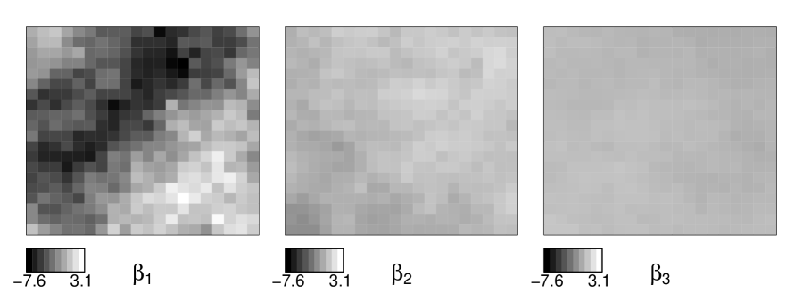
Figure 1: Left to right, the values used for coefficients $\beta_{1}(\bm{s}),\dots,\beta_{3}(\bm{s})$ in the simulation study.

Two parameters were varied to produce six simulation settings. Data were simulated with low ($\rho=0$), medium ($\rho=0.5$), or high ($\rho=0.9$) correlation between the covariates, and with low ($\sigma_{\varepsilon}=0.5$) or high ($\sigma_{\varepsilon}=1$) variance for the random error term. Each setting was used to generate five data sets consisting of 400 observations each. For each data set, estimates were made of the coefficients for three different sample sizes $N$: the full 400 observations, and subsets generated by sampling 100 or 200 unique observations uniformly from the data set. The coefficients were estimated via LAGR and via a VCR model without variable selection as in Section 3. For both estimation methods, the bandwidth parameter was $h=(3/2)N^{-1/6}-0.36$ with a nearest neighbors type bandwidth, meaning the kernel bandwidth was adjusted at each location $\bm{s}_{i}$ to achieve the ratio $\sum_{i^{\prime}=1}^{n}w_{ii^{\prime}}/n=h$.

Simulation settings			MISE $\hat{\beta}_{1}$		MISE $\hat{\beta}_{2}$		MISE $\hat{\beta}_{3}$		MISE $\hat{\beta}_{4}$
$n$	$\rho$	$\sigma_{\varepsilon}$	LAGR	VCR	LAGR	VCR	LAGR	VCR	LAGR	VCR
100	0	0.5	2.16	2.15	0.35	0.36	0.18	0.24	0.15	0.29
		1.0	2.19	2.14	0.38	0.38	0.17	0.28	0.16	0.35
	0.5	0.5	2.36	2.47	0.40	0.35	0.19	0.27	0.26	0.48
		1.0	2.25	2.48	0.44	0.39	0.18	0.34	0.24	0.58
	0.9	0.5	3.00	4.90	0.68	1.16	0.35	1.07	0.70	2.22
		1.0	2.77	5.18	0.61	1.35	0.38	1.37	0.53	2.71
200	0	0.5	1.75	1.72	0.20	0.18	0.09	0.15	0.03	0.10
		1.0	1.79	1.78	0.27	0.21	0.11	0.22	0.05	0.13
	0.5	0.5	1.80	1.75	0.25	0.22	0.12	0.23	0.05	0.15
		1.0	1.84	1.83	0.32	0.28	0.18	0.34	0.07	0.21
	0.9	0.5	2.19	2.37	0.43	0.76	0.36	0.98	0.24	0.75
		1.0	2.25	2.66	0.52	1.10	0.57	1.48	0.32	1.01
400	0	0.5	1.34	1.33	0.18	0.15	0.06	0.06	0.02	0.05
		1.0	1.37	1.35	0.22	0.17	0.08	0.08	0.02	0.05
	0.5	0.5	1.37	1.35	0.20	0.18	0.07	0.09	0.03	0.08
		1.0	1.40	1.39	0.25	0.21	0.09	0.13	0.03	0.09
	0.9	0.5	1.55	1.66	0.41	0.47	0.16	0.36	0.15	0.40
		1.0	1.57	1.84	0.44	0.64	0.17	0.54	0.14	0.46

Table 1: For each setting as a combination of sample size $n$, cross-covariate correlation $\rho$, and error standard deviation $\sigma_{\varepsilon}$, the mean integrated squared error (MISE) of the coefficient estimates, averaged over five independent data sets for each simulation setting. The MISE of $\hat{\beta}_{1},\dots,\hat{\beta}_{4}$ from estimation by local adaptive grouped regularization (LAGR) is compared to that from estimation by locally linear regression without selection (VCR). Highlighting indicates whether LAGR or VCR produced the smaller MISE for each coefficient surface under each simulation setting.

4.2 Simulation Results

The mean integrated squared error (MISE) of the coefficient surface estimates are in Table 1, where the MISE is calculated as $\text{MISE}(\beta_{j})=N^{-1}\sum_{i=1}^{N}\{\hat{\beta}_{j}(\bm{s}_{i})-\beta_{j}(\bm{s}_{i})\}^{2}$. The results in Table 1 are averaged over the five independent data sets for each simulation setting. In general, the coefficients estimated by LAGR were more accurate in terms of MISE than those estimated by VCR. Although the frequency with which MISE was smaller under LAGR than under VCR for estimating $\beta_{1}$ and $\beta_{2}$ was $8$ of $18$ cases each, the improvement by MISE for LAGR over VCR was greater for covariates with smaller influence, with LAGR producing the smaller MISE for $\beta_{3}$ and $\beta_{4}$ in every case. In no case was the MISE for LAGR more than $27\%$ greater than for VCR. The MISE for estimating $\beta_{4}$ with $\rho=0.9$, $\sigma_{\varepsilon}=1.0$, and $n=100$ setting was $5$ times greater for VCR than for LAGR, and under the other simulation settings the greatest improvement for LAGR over VCR tended to be a $2-3$ times reduction in MISE.

With other factors held constant, the MISE for estimating the coefficients tended to be smaller for less influential covariates and under larger sample sizes. On the other hand, the MISE tended to increase with high error variance or increasing correlation between covariates. In terms of MISE, the improvement from estimation by LAGR over VCR was greater for settings with smaller sample sizes, higher correlation between covariates, and greater error variance. In fact, estimation by LAGR was always more accurate than estimation by VCR under high cross-covariate correlation $(\rho=0.9)$.

The frequencies of exact zeros among the estimates of each coefficient for each simulation setting are in Table 2. The frequency of exact zeros in the coefficient estimates generally increased as covariates grew less influential. In particular, the estimates $\hat{\beta}_{1}$ were almost never exactly zero, while the estimates $\hat{\beta}_{3}$ and $\hat{\beta}_{4}$ were exactly zero more often than not. Exact zero coefficient estimates were generally more frequent under smaller sample sizes, greater error variance, and greater cross-covariate correlation. Under high cross-covariate correlation, the frequency of exact zero estimates was roughly equal (and in the neighborhood of $75\%$) for $\beta_{2}$, $\beta_{3}$, and $\beta_{4}$, which indicates that under high cross-covariate correlation, LAGR tended to include only the most influential covariate.

Simulation settings			Zero frequency
$n$	$\rho$	$\sigma_{\varepsilon}$	$\hat{\beta}_{1}$	$\hat{\beta}_{2}$	$\hat{\beta}_{3}$	$\hat{\beta}_{4}$
100	0	0.5	0.00	0.40	0.67	0.76
		1.0	0.00	0.57	0.72	0.80
	0.5	0.5	0.00	0.47	0.68	0.75
		1.0	0.01	0.65	0.77	0.79
	0.9	0.5	0.00	0.76	0.79	0.78
		1.0	0.02	0.84	0.79	0.76
200	0	0.5	0.00	0.28	0.68	0.83
		1.0	0.00	0.39	0.66	0.84
	0.5	0.5	0.00	0.36	0.66	0.81
		1.0	0.00	0.48	0.69	0.84
	0.9	0.5	0.03	0.67	0.74	0.83
		1.0	0.04	0.71	0.69	0.84
400	0	0.5	0.00	0.18	0.56	0.74
		1.0	0.00	0.31	0.64	0.82
	0.5	0.5	0.00	0.24	0.62	0.73
		1.0	0.00	0.36	0.69	0.80
	0.9	0.5	0.02	0.61	0.77	0.73
		1.0	0.02	0.68	0.75	0.80

Table 2: For each setting as a combination of sample size $n$, cross-covariate correlation $\rho$, and error standard deviation $\sigma_{\varepsilon}$, the frequency of exact zeroes in the estimates of $\hat{\beta}_{1},\dots,\hat{\beta}_{4}$ as estimated by local adaptive grouped regularizaton.

5 Data Example

The proposed LAGR estimation method was applied to estimate the coefficients in a VCR model for the price of homes in Boston based on data from the 1970 U.S. census (Harrison and Rubinfeld, 1978; Gilley and Pace, 1996; Pace and Gilley, 1997). The data are the median price of homes sold in 506 census tracts (MEDV), along with the potential covariates CRIM (the per-capita crime rate in the tract), RM (the mean number of rooms for houses sold in the tract), RAD (an index of how accessible the tract is from Boston’s radial roads), TAX (the property tax per $10,000 of property value), and LSTAT (the percentage of the tract’s residents who are considered “lower status”). With the Epanechnikov kernel, the nearest neighbors type bandwidth was set to $h=0.26$.

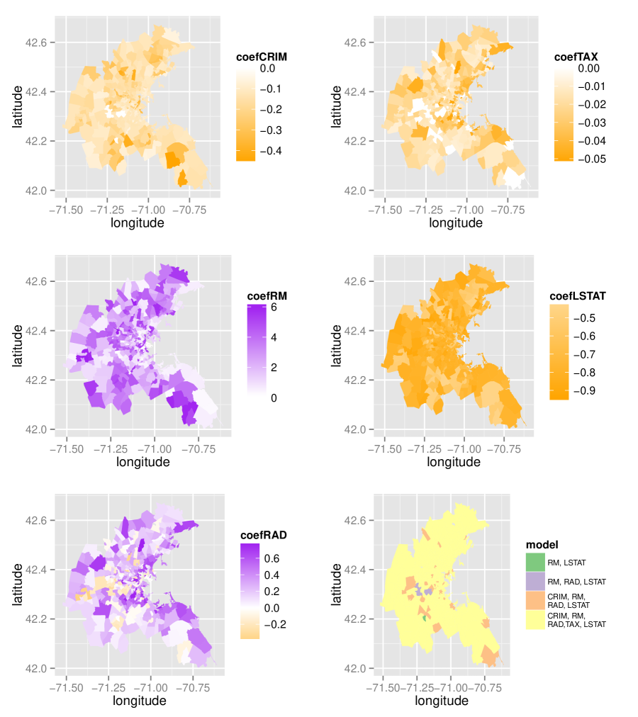
Figure 2: A varying coefficient regression model for the median house price in each census tract in Boston in 1970, estimated by local adaptive grouped regularization. In the left column are the estimated coefficients for covariates CRIM (per-capita crime rate), RM (mean number of rooms per house), and RAD (an index of access to radial roads. In the right column are the estimated coefficients for covariates TAX (property tax per $\$10,000$) and LSTAT (proportion of residents who are “lower status"), and a map indicating which covariates were estimated to have nonzero coefficients in each census tract.

The estimates of the local coefficients are plotted in the first five panels of Figure 2 and are summarized in Table 3. The estimated coefficients of CRIM and LSTAT were everywhere negative or exactly zero, suggesting that the crime rate and proportion of “lower-status" individuals were associated with a lower median house price. Meanwhile, the coefficient of RM was everywhere estimated to be positive, so the more rooms in the average house was everywhere associated with a higher median house price. The coefficient of TAX was negative in most census tracts, but was estimated to be exactly zero in 50 tracts, indicating no discernable effect of the property tax rate on house prices in those tracts. The coefficient of RAD is positive in some areas and negative in others. This indicates that there are parts of Boston where access to radial roads is associated with a greater median house price and parts where it is associated with a lesser median house price. The bottom right panel of Figure 2 shows which covariates were estimated to have a nonzero coefficient in each tract. There were 471 tracts where all LAGR estimated that all the covariates had a nonzero coefficient, 43 tracts where all covariates except for TAX were estimated to have nonzero coefficients, six tracts where the coefficients of CRIM and TAX were estimated to be zero, and one tract where the coefficients of CRIM, RAD, and LSTAT were estimated to be zero.

Covariate	Mean	Standard dev.	Zero coef. count
CRIM	-0.15	0.07	7
RM	2.56	1.68	0
RAD	0.21	0.25	1
TAX	-0.02	0.01	50
LSTAT	-0.73	0.13	0

Table 3: The mean, standard deviation, and count of zeros among the estimates of the local coefficients in a model for the median house price in 506 census tracts in Boston, with coefficients selected and fitted by local adaptive grouped regularization. The covariates are CRIM (per capita crime rate in the census tract), RM (average number of rooms per home sold in the census tract), RAD (an index of the tract’s access to radial roads), TAX (property tax per USD10,000 of property value), and LSTAT (percentage of the tract’s residents who are considered “lower status").

6 Extension to Generalized Linear Regression

6.1 Local GLM and Local Quasi-likelihood Estimation

Generalized linear models (GLMs) extend the linear regression model to a response variable following any distribution in the exponential family (McCullagh and Nelder, 1989). As is the case for the local linear regression model, we now consider local GLM coefficients as smooth functions of location (Cai et al., 2000). Suppose the response variable $Y$ is from an exponential family distribution with $E\left\{y(\bm{s})|\bm{x}(\bm{s})\right\}=\mu(\bm{s})=b^{\prime}\left(\theta(\bm{s})\right)$, $\theta(\bm{s})=(g\circ b^{\prime})^{-1}\left(\eta(\bm{s})\right)$, $\eta(\bm{s})=\bm{x}(\bm{s})^{T}\bm{\beta}(\bm{s})=g\left(\mu(\bm{s})\right)$, $\text{\text{Var}}\left\{y(\bm{s})|\bm{x}(\bm{s})\right\}=b^{\prime\prime}\left(\theta(\bm{s})\right)$, and link function $g(\cdot)$. Then the probability density is

$$f\left(y(\bm{s})|\bm{x}(\bm{s}),\theta(\bm{s})\right)=c\left(y(\bm{s})\right)\times\exp\left\{\theta(\bm{s})y(\bm{s})-b\left(\theta(\bm{s})\right)\right\}.$$

If $g^{-1}(\cdot)=b^{\prime}(\cdot)$, then the composition $(g\circ b^{\prime})(\cdot)$ is the identity function. This particular $g$ is called the canonical link. Assuming the canonical link, all that is required is to specify the mean-variance relationship via the variance function, $V\left(\mu(\bm{s})\right)$. Then the local coefficients can be estimated by maximizing the local quasi-likelihood

$$\mathcal{\ell}^{*}\left(\bm{\zeta}(\bm{s})\right) =\sum_{i=1}^{n}K_{h}\left(\|\bm{s}-\bm{s}_{i}\|\right)Q\left(g^{-1}\left(\bm{z}_{i}^{T}\bm{\zeta}(\bm{s})\right),Y_{i}\right).$$ (7)

The local quasi-likelihood (7) generalizes the local log-likelihood (3) that was used to estimate coefficients in the local linear regression. The local quasi-likelihood (7) is concave, and is defined in terms of its derivative, the local quasi-score function $\left(\partial/\partial\mu\right)Q(\mu,y)=(y-\mu)\{V(\mu)\}^{-1}$. The local quasi-likelihood is maximized by setting the local quasi-score function to zero:

$$(\partial/\partial\bm{\zeta})\mathcal{\ell}^{*}\left(\hat{\bm{\zeta}}(\bm{s})\right) =\sum_{i=1}^{n}K_{h}\left(\|\bm{s}-\bm{s}_{i}\|\right)\left(y_{i}-\hat{\mu}(\bm{s}_{i};\bm{s})\right)\left\{V\left(\hat{\mu}(\bm{s}_{i};\bm{s})\right)\right\}^{-1}\bm{z}_{i}=\bm{0}_{3p},$$ (8)

where $\hat{\mu}(\bm{s}_{i};\bm{s})=g^{-1}\left(\bm{z}_{i}^{T}\hat{\bm{\zeta}}(\bm{s})\right)$ is the mean at location $\bm{s}_{i}$ evaluated at the estimated coefficients $\hat{\bm{\zeta}}(\bm{s})$ at location $\bm{s}$. The asymptotic distribution of the local coefficients in a varying-coefficient GLM with a one-dimensional effect-modifying parameter are given in Cai et al. (2000). For coefficients that vary in the two dimensions, the arguments in the proof of Theorem 1 of Cai et al. (2000) can be extended to show that the distribution of the estimated local coefficients is:

$$\left\{nh^{2}f(\bm{s})\right\}^{1/2}\left[\tilde{\bm{\beta}}(\bm{s})-\bm{\beta}(\bm{s})-(1/2)\kappa_{0}^{-1}\kappa_{2}h^{2}\left\{\nabla_{uu}^{2}\bm{\beta}(\bm{s})+\nabla_{vv}^{2}\bm{\beta}(\bm{s})\right\}\right]$$

$$\xrightarrow{{D}}N\left(\bm{0},\kappa_{0}^{-2}\nu_{0}\bm{\Gamma}(\bm{s})^{-1}\right).$$

where $\bm{\Gamma}\left(\bm{s}\right)=E\left\{\rho\left(\bm{s},\bm{X}(\bm{s})\right)\bm{X}(\bm{s})\bm{X}(\bm{s})^{T}|\bm{s}\right\}$,
$\rho(\bm{s},\bm{z})=\left[g_{1}\left(\mu(\bm{s},\bm{z})\right)\right]^{2}Var\left\{Y(\bm{s})|\bm{X}(\bm{s}),\bm{s}\right\}$, $g_{1}(\cdot)=g^{\prime}_{0}(\cdot)/g^{\prime}(\cdot)$, and $g_{0}(\cdot)$ is the canonical link function. So when the canonical link is used, $\rho(\bm{s},\bm{z})=V\left(\mu(\bm{s},\bm{z})\right)$.

6.2 LAGR Penalized Local Likelihood and Oracle Properties

Whereas the method of LAGR for local linear regression uses a penalized local likelihood, LAGR for GLMs uses a penalized negative local quasi-likelihood:

$$\mathcal{J}\left(\bm{\zeta}(\bm{s})\right) =-\mathcal{\ell}^{*}\left(\bm{\zeta}(\bm{s})\right)+\mathcal{P}\left(\bm{\zeta}(\bm{s})\right)$$

$$=-\sum_{i=1}^{n}K_{h}\left(\|\bm{s}-\bm{s}_{i}\|\right)Q\left(g^{-1}\left(\bm{z}_{i}^{T}\bm{\zeta}(\bm{s})\right),Y_{i}\right)+\sum_{j=1}^{p}\phi_{j}(\bm{s})\|\bm{\zeta}_{(j)}(\bm{s})\|.$$

Further, let $\phi_{j}(\bm{s})=\lambda_{n}\|\tilde{\bm{\zeta}}_{(j)}(\bm{s})\|^{-\gamma}$, where $\lambda_{n}>0$ is a the local tuning parameter applied to all coefficients at location $\bm{s}$ and $\tilde{\bm{\zeta}}_{(j)}(\bm{s})$ is the vector of unpenalized local coefficients. In addition to the definitions and conditions of Section 3.2, let

$$\bm{\Gamma}_{(a)}\left(\bm{s}\right)=E\left\{\rho\left(\bm{s},\bm{X}_{(a)}(\bm{s})\right)\bm{X}_{(a)}(\bm{s})\bm{X}_{(a)}(\bm{s})^{T}|\bm{s}\right\}$$

and assume the following regularity conditions:

• The functions $g^{\prime\prime\prime}\left(\bm{s}\right)$, $\nabla\bm{\Gamma}\left(\bm{s}\right)$, $\nabla\bm{\Gamma}_{(a)}\left(\bm{s}\right)$, $V\left(\mu\left(\bm{s},\bm{z}\right)\right)$, and $V^{\prime}\left(\mu\left(\bm{s},\bm{z}\right)\right)$ are continuous at $\bm{s}$.

• The function $\left(\partial^{2}/\partial\mu^{2}\right)Q\left(g^{-1}\left(\mu\right),y\right)<0$ for $\mu\in\mathbb{R}$ and $y$ in the range of the response.

These additional conditions are not uncommon in the nonparametric regression literature (see, e.g., conditions (1) and (2) of Cai et al. (2000)). Condition (C.8) is needed for the Taylor’s expansion of the local quasi-likelihood. Condition (C.9) assures that the local quasi-likelihood is concave and has a unique maximizer.

Theorem 3 (Asymptotic normality).

Under (C.1)–(C.10),

$$\left\{nh^{2}f(\bm{s})\right\}^{1/2}\left[\hat{\bm{\beta}}_{(a)}(\bm{s})-\bm{\beta}_{(a)}(\bm{s})-\left(2\kappa_{0}\right)^{-1}\kappa_{2}h^{2}\left\{\nabla_{uu}^{2}\bm{\beta}_{\left(a\right)}(\bm{s})+\nabla_{vv}^{2}\bm{\beta}_{\left(a\right)}(\bm{s})\right\}\right]$$

$$\xrightarrow{d}N\left(0,\kappa_{0}^{-2}\nu_{0}\bm{\Gamma}_{(a)}(\bm{s})^{-1}\right)$$

Theorem 4 (Selection consistency).

Under (C.1)–(C.10), if $j>p_0(𝐬$

References

- Akaike (1973) Akaike, H. (1973). Information theory and an extension of the maximum likelihood principle. In B. Petrov and F. Csaki (Eds.), 2nd International Symposium on Information Theory, pp. 267–281.
- Antoniadas et al. (2012) Antoniadas, A., I. Gijbels, and A. Verhasselt (2012). Variable selection in varying-coefficient models using P-splines. Journal of Computational and Graphical Statistics 21, 638–661.
- Cai et al. (2000) Cai, Z., J. Fan, and R. Li (2000). Efficient estimation and inferences for varying-coefficient models. Journal of the American Statistical Association 95, 888–902.
- Cleveland and Grosse (1991) Cleveland, W. and E. Grosse (1991). Local regression models. In J. Chambers and T. Hastie (Eds.), Statistical Models in S. Wadsworth and Brooks/Cole.
- Efron (2004) Efron, B. (2004). The estimation of prediction error: covariance penalties and cross-validation. Journal of the American Statistical Association 99, 619–632.
- Fan and Gijbels (1996) Fan, J. and I. Gijbels (1996). Local Polynomial Modeling and its Applications. Chapman and Hall, London.
- Fan and Zhang (1999) Fan, J. and W. Zhang (1999). Statistical estimation in varying coefficient models. Annals of Statistics 27, 1491–1518.
- Geyer (1994) Geyer, C. J. (1994). On the asymptotics of constrained -estimation. Annals of Statistics 22, 1993–2010.
- Gilley and Pace (1996) Gilley, O. and R. K. Pace (1996). On the Harrison and Rubinfeld data. Journal of Environmental Economics and Management 31, 403–405.
- Harrison and Rubinfeld (1978) Harrison, D. and D. L. Rubinfeld (1978). Hedonic housing prices and the demand for clean air. Journal of Environmental Economics and Management 5, 81–102.
- Hastie and Loader (1993) Hastie, T. and C. Loader (1993). Local regression: automatic kernel carpentry. Statistical Science 8, 120–143.
- Hastie and Tibshirani (1993) Hastie, T. and R. Tibshirani (1993). Varying-coefficient models. Journal of the Royal Statistical Society Series B 55, 757–796.
- Hurvich et al. (1998) Hurvich, C. M., J. S. Simonoff, and C.-L. Tsai (1998). Smoothing parameter selection in nonparametric regression using an improved Akaike information criterion. Journal of the Royal Statistical Society Series B 60, 271–293.
- Knight and Fu (2000) Knight, K. and W. Fu (2000). Asymptotics for Lasso-type estimators. Annals of Statistics 28, 1356–1378.
- Mallows (1973) Mallows, C. (1973). Some comments on . Technometrics 15, 661–675.
- McCullagh and Nelder (1989) McCullagh, P. and J. Nelder (1989). Generalized Linear Models, Second Edition. Taylor and Francis.
- Pace and Gilley (1997) Pace, R. K. and O. Gilley (1997). Using the spatial configuration of the data to improve estimation. Journal of Real Estate Finance and Economics 14, 333–340.
- R Core Team (2014) R Core Team (2014). R: A Language and Environment for Statistical Computing. R Foundation for Statistical Computing, Vienna, Austria. URL http://www.R-project.org/.
- Samiuddin and el Sayyad (1990) Samiuddin, M. and G. M. el Sayyad (1990). On nonparametric kernel density estimates. Biometrika 77, 865–874.
- Stein (1981) Stein, C. (1981). Estimation of the mean of a multivariate normal distribution. Annals of Statistics 9, 1135–1151.
- Sun et al. (2014) Sun, Y., H. Yan, W. Zhang, and Z. Lu (2014). A semiparametric spatial dynamic model. Annals of Statistics 42, 700–727.
- Tibshirani (1996) Tibshirani, R. (1996). Regression shrinkage and selection via the Lasso. Journal of the Royal Statistical Society Series B 58, 267–288.
- Wang and Leng (2008) Wang, H. and C. Leng (2008). A note on adaptive group Lasso. Computational Statistics and Data Analysis 52, 5277–5286.
- Wang and Xia (2009) Wang, H. and Y. Xia (2009). Shrinkage estimation of the varying coefficient model. Journal of the American Statistical Association 104, 747–757.
- Wang et al. (2008) Wang, L., H. Li, and J. Z. Huang (2008). Variable selection in nonparametric varying-coefficient models for analysis of repeated measurements. Journal of the American Statistical Association 103, 1556–1569.
- Wang et al. (2008) Wang, N., C.-L. Mei, and X.-D. Yan (2008). Local linear estimation of spatially varying coefficient models: an improvement on the geographically weighted regression technique. Environment and Planning A 40, 986–1005.
- Yuan and Lin (2006) Yuan, M. and Y. Lin (2006). Model selection and estimation in regression with grouped variables. Journal of the Royal Statistical Society Series B 68, 49–67.
- Zou (2006) Zou, H. (2006). The adaptive Lasso and its oracle properties. Journal of the American Statistical Association 101, 1418–1429.
Appendix A Proofs of Theorems 1–2
Proof of Theorem 1
Proof.
Let and . Then, we have
The limiting behavior of the last term differs between the cases
and .
Case : If , then
and
. Thus,
Case : If , then . Since , if , then . Thus, if , then
On the other hand, if , then . Thus, the limit of is the same as the limit of where if for some , and
otherwise. It follows that is convex and has a unique minimizer, called . Let and be, respectively, the subvectors of corresponding to the true nonzero coefficients and true zero coefficients. Then
and By epiconvergence, the minimizer of the limiting function is the limit of the minimizers (Geyer, 1994; Knight and Fu, 2000). Since, by Lemma 2 of Sun et al. (2014),
the result of Theorem 1 follows. ∎
Proof of Theorem 2
Proof.
The proof is by contradiction. Without loss of generality we consider only the th covariate group. Assume . Then is differentiable w.r.t. and is minimized where
Thus,