The Role of the Magnetorotational Instability in Massive Stars

Abstract

The magnetorotational instability (MRI) is key physics in accretion disks and is widely considered to play some role in massive–star core collapse. Models of rotating massive stars naturally develop very strong shear at composition boundaries, a necessary condition for MRI instability, and the MRI is subject to triply–diffusive destabilizing effects in radiative regions. We have used the MESA stellar evolution code to compute magnetic effects due to the Spruit–Taylor mechanism and the MRI, separately and together, in a sample of massive star models. We find that the MRI can be active in the later stages of massive star evolution, leading to mixing effects that are not captured in models that neglect the MRI. The MRI and related magneto–rotational effects can move models of given ZAMS mass across “boundaries” from degenerate CO cores to degenerate O/Ne/Mg cores and from degenerate O/Ne/Mg cores to iron cores, thus affecting the final evolution and the physics of core collapse. The MRI acting alone can slow the rotation of the inner core in general agreement with the observed “initial" rotation rates of pulsars. The MRI analysis suggests that localized fields $\sim 10^{12}$ G may exist at the boundary of the iron core. With both the ST and MRI mechanisms active in the 20 M_⊙ model, we find that the helium shell mixes entirely out into the envelope. Enhanced mixing could yield a population of yellow or even blue supergiant supernova progenitors that would not be standard SN IIP.

1. Introduction

One of the major unsolved problems of stellar evolution is the effect of differential rotation on the magnetic field structure of stars and the feedback of that magnetic field on the stellar structure and evolution. The role of rotation in stars is well-studied if not fully understood (Von Zeipel, 1924; Goldreich & Schubert, 1967; Fricke, 1969; Tassoul, 1978; Endal & Sofia, 1981; Maeder, 2009; Maeder & Meynet, 2014). Some of that work includes the effects of magnetic fields (Maeder, 2009, and references therein), but this remains a major challenge requiring fully three-dimensional studies. Even the status of the solar rotation and magnetic field remains a major issue (Christensen-Dalsgaard et al., 1996; Howe, 2009). The late stages of stellar evolution where direct relevant observations are scarce is even more of a challenge. The actual amount of angular momentum and magnetic field of the iron core has obvious implications for the creation of new–born neutron stars and for black holes.

Spruit (1999, 2002) presented various magnetic instabilities that could be involved in stellar evolution and prescriptions for treating them, including the Tayler instability (Tayler, 1973) and the magneto–rotational instability (MRI; Velikhov, 1950; Chandrasekhar, 1960; Acheson, 1978; Balbus & Hawley, 1991, 1998). Spruit emphasized the nature and role of the Tayler instability in which a toroidal field could be perturbed, twisted, and sheared to produce a radial field. This is a pinch-type instability of a toroidal magnetic field in differentially rotating stellar radiative zones that is predicted to result in large-scale fluid motion in the star. Spruit gave a prescription for the equilibrium field structure, in particular the ratio of the radial and toroidal fields, and for the magnetic viscosity that would result from the drag associated with the radial component of the field interacting with shear in the star. We refer to these effects collectively as the Spruit–Tayler (ST) mechanism. Heger et al. (2005) (see also Maeder & Meynet, 2004; Petrovic et al., 2005; Cantiello et al., 2007; Suijs et al., 2008; Paxton et al., 2011, 2013; Brott et al., 2011; Ekström et al., 2012; Chatzopoulos & Wheeler, 2012; Yoon et al., 2012) incorporated the ST magnetic viscosity prescription in a one–dimensional stellar evolution code that had previously been used to explore the effect on angular momentum transport of a wide variety of classical fluid instabilities (Heger et al., 2000). Heger et al. (2005) concluded that the ST magnetic viscosity would tend to damp the rotation rate of the iron core that formed in the final stages of evolution of massive stars by a factor of 30 - 50 compared to computations that did not account for magnetic torques and that more massive stars would have more rapidly rotating iron cores. A variety of issues concerning the ST mechanism remain open. We return to that topic in §4.

Although the MRI has been thoroughly explored in the context of accretion disks, it also applies to quasi-spherical objects, e.g. stars (Balbus & Hawley, 1994). The MRI is widely considered to play some role in core collapse (Akiyama et al., 2003; Masada et al., 2006, 2007; Obergaulinger et al., 2009; Sawai & Yamada, 2014), but its role in stellar evolution has been substantially neglected. This is in part because a threshold shear is required to trigger the MRI and the MRI tends to be stabilized by strong thermal and composition gradients (Maeder, 2009). On the other hand, models of rotating massive stars naturally develop strong shear at composition boundaries, and the MRI is subject to triply-diffusive destabilizing effects in radiative regions (Acheson, 1978; Menou et al., 2004). The MRI grows exponentially rapidly when unstable and can be active in the Sun (Parfrey & Menou, 2007; Masada, 2011; Kagan & Wheeler, 2014). We argue here that the MRI should also be considered in the context of the evolution of massive stars.

Heger et al. (2005) neglect the MRI, but the resulting models tend to give very strong radial gradients in the angular velocity in the final stages of the evolution (see Figures 2 and 3 in Heger et al. for the corresponding specific angular momentum gradient distributions). These sharp gradients arise at the composition boundaries of the “onion-skin" layers that are also the boundaries between (possibly extinct) convective cores and outer radiative layers that may once themselves have been involved in convective burning. These sharp boundaries are stabilized against Kelvin–Helmholtz instabilities by the associated composition gradients, but they may be unstable to interface dynamos (Brun et al., 2005) or the MRI. One question is whether or not such sharp gradients in angular velocity would have developed in the first place had the MRI been considered as the star evolved on and after the main sequence.

Where in the geometry various instabilities occur is a major issue. As noted by Spruit (1999), the Tayler instability disappears on the equator and shows its most characteristic behavior near the rotation axis. The MRI may be most active near the equator in radiative shearing regions where the shear is strong and weaker at the poles, but in the tachocline and convective envelope of the Sun the MRI tends to be supressed at low latitudes (Parfrey & Menou, 2007; Masada, 2011; Kagan & Wheeler, 2014). In the following, we will neglect these considerations due to the restrictions of a spherically–symmetric evolution code, but return to them in §4.

In §2 we present the instability criterion for the MRI, the resulting expressions for viscosity and diffusion coefficients that transport angular momentum and mix compositions, and our treatment of the growth and saturation of the magnetic field. Section 3 describes our use of the MESA code and gives our results, and §4 presents a discussion and conclusions.

2. Physical Properties of the ST and MRI Mechanisms

We first define a number of terms that will be employed in the subsequent discussion. The angular velocity is $\Omega$ and $q=d\ln\Omega/d\ln r$ is the radial shear. The Alfvén frequency is $\omega_{A}$. Assuming the toroidal field to dominate, the Alfvén frequency and Alfvén velocity are:

$$\omega_{\rm A}=\frac{{\rm v_{A}}}{r}=\frac{B_{\phi}}{\sqrt{4\pi\rho}r}.$$ (1)

The terms $N_{T}$ and $N_{\mu}$ are the thermal and composition components of the Brunt-Väisälä frequency,

$$N_{T}^{2}=\frac{g\delta}{H_{p}}\left(\nabla_{\rm ad}-\nabla_{\rm rad}\right),$$ (2)

and

$$N_{\mu}^{2}=g\phi\left|\frac{\partial\ln\mu}{\partial r}\right|,$$ (3)

where $\nabla_{\rm ad}$ and $\nabla_{\rm rad}$ are the adiabatic and radiative gradients, $H_{P}$ is the pressure scale height, $g$ is the local gravity, $\mu$ is the mean molecular weight, $\delta=-\left(\partial\ln\rho/\partial\ln T\right)_{P,\mu}$, $\phi=\left(\partial\ln\rho/\partial\ln\mu\right)_{P,T}$, where $\rho$, T, and P are the local density, temperature and pressure, respectively. The thermal diffusivity is dominated by radiative transport, and is given by

$$\kappa=\frac{16\sigma T^{3}}{3\kappa_{R}\rho^{2}c_{P}},$$ (4)

where $\gamma$ is the ratio of specific heats and $\kappa_{R}$ is the radiative opacity. The magnetic resistivity, $\eta$, is given by

$$\eta\approx 5.2\times 10^{11}\frac{\ln\Lambda}{T^{3/2}}\,{\rm cm^{2}}\,{\rm s^{-1}},$$ (5)

(Spitzer, 2006) where $\ln\Lambda$ is the Coulomb logarithm

$$\ln\Lambda\approx\begin{cases}-17.4+1.5\ln T-0.5\ln\rho&\,T<1.1\times 10^{5}\,\rm{K},\\ -12.7+\ln T-0.5\ln\rho&\,T>1.1\times 10^{5}\,\rm{K}.\end{cases}$$ (6)

after translating into cgs units. In the current work, we assume the thermal viscosity is negligible compared to $\kappa$ and $\eta$ (Menou et al., 2004).

2.1. Instability and Growth Rate

The appropriate expressions for the instability criteria have terms that depend on radial and on lateral gradients. The latter cannot be captured in a one–dimensional code like MESA, so we address only the spherical radial components of the instability criteria.

2.1.1 ST Instability

For the ST instability, a minimum initial magnetic field is required for growth. In our calculations of the ST dynamo process, we assume that this minimum field is present. In order for the overall ST dynamo process to work, however, a significant shear is required to overcome the effects of both thermal and compositional buoyancy. Following Spruit (2002), the shear condition for the ST process to operate may be expressed in our notation as

$$|q|>q_{\rm min}\equiv\left(\frac{N_{\rm lim}}{\Omega}\right)^{3/2}\left(\frac{\eta}{r^{2}\Omega}\right)^{1/4},$$ (7)

where

$$N_{\rm lim}^{2}=\left(\frac{\eta}{\kappa}\right)\max(N_{T}^{2},0)+\max(N_{\mu}^{2},0).$$ (8)

Note that the sign of the shear is not important for the ST dynamo. This is because the only effect of the shear in the ST dynamo process is in winding up the poloidal field produced by the ST instability, and the field winding process depends only on the magnitude of the shear, not its sign.

2.1.2 MRI Instability

Following Balbus & Hawley (1991, 1998), Akiyama et al. (2003), Menou et al. (2004) and (Kagan & Wheeler, 2014), we can write the local instability criterion for the MRI in typical conditions in stars where the magnetic diffusivity $\eta$ is significantly smaller than the thermal diffusivity $\kappa$ as

$$\left(\frac{\eta}{\kappa}\right)N_{T}^{2}+N_{\mu}^{2}+2q\Omega^{2}<0.$$ (9)

In the absence of the Brunt–Väisälä terms in Equation (9), the instability criterion for the MRI is simply $2q\Omega^{2}<0$; that is, the system is unstable when $q<0$, i.e., the angular velocity decreases outward. The component of the Brunt–Väisälä frequency associated with composition gradients, $N_{\mu}^{2}$, is nearly always a stabilizing term in stars since the molecular weight almost always decreases monotonically outward. An exception arises in §3.2 where we find a composition inversion with silicon overlying oxygen in the model with ZAMS mass of 11 M_⊙. The thermal component of the Brunt–Väisälä frequency varies with the stellar structure. In convective regions, $N_{T}^{2}$ is negative and the convective overturn promotes the MRI. In radiative regions, $N_{T}^{2}$ is positive and this term will then tend to oppose the MRI instability. The thermal buoyancy term is, however, diminished by diffusive effects. For small–scale perturbations, perturbed fluid elements reach thermal equilibrium with the surroundings more quickly, thus reducing thermal buoyancy and the associated stabilizing influence. The magnetic diffusivity will tend to promote stability because the tendency to amplify the field will diminish. Note that the latter is a very subtle effect, since that is the only indirect effect of the magnetic field. As long as the magnetic field is weak compared to the effects of rotation, $\omega_{A}<<\Omega$, the instability criterion of Equation (9) does not depend on the strength of the magnetic field, one of the special properties of the MRI (Balbus & Hawley, 1998).

Note that that the precise definition of the “reduced" $N_{T}$ depends on the particular instability. In the derivation of the MRI presented in Kagan & Wheeler (2014), the term that we adopt in Equation (9), $N_{T,\rm reduced}^{2}=(\eta/\kappa)N_{T}^{2}$, corresponds to the instability criterion for the diffusive small–scale MRI. Menou et al. (2004) present other instability criteria for which the appropriate reduced value is different. Although it is reasonable in the ambiance we explore in which $\eta<<\kappa$, our expression would give unrealistically high estimates for the effects of buoyancy if $\eta>>\kappa$, giving $N_{T,\rm reduced}>>N_{T}$.

While the growth rate in the ST mechanism depends on the field strength in a manner that leads to predictions of the ratio of the resulting radial and toroidal field (§2.3), the MRI is different in a fundamental way. If the field strength is below saturation, the growth rate of the MRI depends only on the shear, not on the strength of the magnetic field. In regions unstable to the MRI, the field should grow exponentially rapidly at the rate $q\Omega$. The growth rate for the MRI is likely to be much more rapid than that for the ST instability if the initial conditions correspond to a weak magnetic field, $\omega_{A}<<\Omega$.

2.2. Viscosity and Diffusion Coefficients

In MESA, all instabilities (including ST, Eddington–Sweet (meridional circulation), Goldrich–Schubert–Fricke) and the MRI are treated as diffusive processes that diffuse angular momentum or species (mixing). The net viscosity, $\nu$, is assumed to be the linear sum of the viscous diffusion coefficients $\nu_{i}$, corresponding to estimates of the diffusion coefficient for each individual process, $i$. Whether or not the diffusive effects associated with these various instabilities can truly be added in this simple linear way deserves deeper consideration, but that is beyond the scope of this work. Following Spruit (2002), the azimuthal stress, $S$, generated by the field produced by either ST or MRI can be related to an effective magnetic viscosity, ${\nu_{\rm mag}}$, by

$$S=\frac{B_{r}B_{\phi}}{4\pi}=\rho q\Omega\nu_{\rm mag}.$$ (10)

This viscosity is explicitly an “effective magnetic viscosity" that is determined by the global magnetic structure of the star and very specifically is not in any way related to the microphysics of “molecular viscosity" in the star.

2.2.1 ST Viscosity

For the ST process, the magnetic field components are first constrained by various physical arguments. The resulting prescriptions for $B_{r}$ and $B_{\phi}$ are then incorporated in Equation (10) to evaluate the effective viscosity (Spruit, 1999, 2002). The strength of the magnetic field components can be cast in a form in which the ST viscosity, $\nu_{\rm mag,ST}$, is treated as a variable (§2.3.1).

Our calculations for the magnetic viscosity, $\nu_{\rm mag,ST}$, corresponding to the ST mechanism are identical to those in Heger et al. (2005) that are incorporated in MESA. The form of the equation for the effective ST viscosity depends on the signs of $N_{T}^{2}$ and $N_{\mu}^{2}$ and the strength of thermal diffusion, $\kappa$. In radiative regions, where both $N_{T}^{2}$ and $N_{\mu}^{2}$ are positive, we apply the effective viscosity calculated in Equations (34)-(37) of Spruit (2002). In semiconvective regions where $N_{T}^{2}<0$ and $N_{\mu}^{2}>0$, we apply Equations (6)-(9) of Heger et al. (2005). In thermohaline regions where $N_{T}^{2}>0$ and $N_{\mu}^{2}<0$, we apply Equation (36) of Spruit (2002), which corresponds to his “Case 1."

2.2.2 MRI Viscosity

Dimensionally, $B\sim q\Omega r\sqrt{4\pi\rho}$ (§2.3.2). Assuming the toroidal field to dominate, we can obtain a formal expression for the magnetic viscosity corresponding to the MRI by substituting this expression into Equation (10)

$$\nu_{\rm mag,MRI}=\frac{B_{r}B_{\phi}}{4\pi\rho|q|\Omega}=\left(\frac{B_{r}}{B_{\phi}}\right)|q|\Omega r^{2},$$ (11)

where the absolute value sign is used to ensure that $\nu$ is positive. We have not defined precisely what we mean by $B_{r}$ and $B_{\phi}$ in this context. We return to this expression in §2.3.2.

To estimate the viscosity corresponding to the MRI, we have recourse to shearing–box simulations. In accretion disks, the rotation is supersonic and the field produced by the MRI is limited to be less than the value corresponding to equipartition with the local gas pressure, $\rho(\omega_{\rm A}r)^{2}\sim P_{\rm gas}$. Because the components of the magnetic field are turbulent, temporal and spatial averaging of simulation data is needed to obtain an accurate estimate of field components and their products. The normalized total magnetic pressure in a simulation can be expressed as $<B^{2}>/(8\pi P_{0})$, where $P_{0}$ is the maximum magnetic pressure that can be produced by the MRI at saturation. We adopt $P_{0}=P_{\rm gas}$. If the radiation pressure, $P_{\rm rad}$, is significant, this expression should be replaced with $P_{0}=P_{\rm gas}+P_{\rm rad}$ to produce the correct normalization (Shi et al., 2010). In the calculations here, the gas pressure and degeneracy pressure typically exceed the radiation pressure by factors of at least several in the inner core. The addition of rotation and mixing tends to increase $P_{\rm gas}/P_{\rm rad}$. We have neglected $P_{\rm rad}$ in our estimate of $\alpha$ in the current work. We argue that the corresponding normalization in the subsonic shearing conditions relevant to stars is $P_{0}=\rho(q\Omega r)^{2}$. We then assume that the appropriately normalized magnetic field components are the same in both accretion disks and in stars.

A stress efficiency parameter, $\alpha$, can then be defined as

$$\alpha\equiv\frac{S}{P_{0}}=\frac{<B_{r}B_{\phi}>}{4\pi P_{0}},$$ (12)

where $<B_{r}B_{\phi}>$ is a suitable spatial and temporal average of the product of the field components. As just argued, the normalization is $P_{0}=P_{\rm gas}$ for an accretion disk and $P_{0}=\rho(q\Omega r)^{2}$ for stars. We assume that the normalized parameter $\alpha$ is the same in both disks and stars.

In local shearing–box simulations, the typical value of $\alpha$ is in the range 0.01 to 0.05 (Hawley et al., 2011, and references therein). Global simulations may produce slightly larger values of $\alpha$, perhaps as large as 0.1 (Hawley et al., 2011). We adopt $\alpha=0.02$ as representative. Using the right hand side of Equation (10) and the definition of $\alpha$ in the left hand side of Equation (12) yields an effective viscosity for the MRI of

$$\nu_{\rm MRI}=0.02|q|\Omega r^{2}.$$ (13)

We apply Equation (13) for all values of $N_{T}^{2}$ and $N_{\mu}^{2}$ without modification as long as the instability criterion (9) is satisfied. The issue of how the MRI works in semiconvective or thermohaline regions requires further work that is beyond the scope of this paper. The prescription for viscosity is not modified in semiconvective or thermohaline regions in the current work.

We have considered other physical conditions and associated prescriptions for the effective viscosity of the MRI. Spruit (1999) gives a prescription for the viscosity associated with the MRI (his Equation 31)

$$\nu_{\rm MRI}\sim 0.2|q|\kappa\left(\frac{\Omega}{N_{T}}\right)^{2}.$$ (14)

Spruit notes that this viscosity may be relatively small, but that his conclusion is preliminary pending numerical simulations of the non–linear development. This prescription was based on the assumption that conditions are held very near those corresponding to the onset of the linear instability. It is not clear to us that the system under consideration will maintain this marginal condition. We have, rather, invoked estimates corresponding to something like saturation as revealed by simulations. We have, however, run one 15M_⊙ model (§3.3) with the prescription of Equation (14) and find that it can be comparable to, or even exceed the prescription we adopt in Equation (13).

Another concern is that the instability criterion, Equation (9), specifically invokes the destabilizing effect of thermal diffusion. The question arises as to whether or not the effectiveness of the MRI in providing a viscosity is also limited by the constraint of significant thermal diffusion. Since the growth time of the magnetic field is given by the shear, the Maxwell stress is of order the Reynolds stress, $S\sim\rho\ell_{r}\ell_{\phi}\sigma^{2}$, where $\ell_{r}$ and $\ell_{\phi}$ are characteristic length scales in the radial and azimuthal directions and $\sigma\sim q\Omega$. If to maintain the growth of the MRI, the length scales are restricted to be sufficiently small that thermal diffusion is active, then the effectve stress and associated viscosity might be also limited. Suppose, for example, that $\ell_{\phi}\sim r$ ( or a pressure scale height), but that $\ell_{r}$ is restricted by the condition of effective thermal diffusivity. The latter could be expressed by writing $k^{2}\kappa\sim N$ where $k$ is the wavenumber of the maximally destabilized mode and $N$ is the Brunt-Väisälä frequency. The constraint on the length scale can thus be expressed as $\ell_{r}\sim\sqrt{\kappa/N}$ and the stress as $S\sim\rho q^{2}\Omega^{2}r\sqrt{\kappa/N}$. The associated viscosity would then be

$$\nu\sim|q|\Omega r\sqrt{\kappa/N},$$ (15)

smaller than we adopted in Equation (13) by a factor of roughly $\sqrt{\kappa/N}/r$. We have been somewhat loose in this discussion with the exact nature of the Brunt-Väisälä frequency, N. The relevant choice would seem to be the thermal component, $N_{T}$, since this sets the relevant buoyancy timescale and, in the absence of thermal destablizing effects, dominates the composition term. Conditions for which $N_{T}^{2}<0$ will be convective and the effective convective dynamic viscosity would then dominate other effects. We have adopted the prescription of Equation (15) in a model of a 15 M_⊙star (§3.3) in regions that are unstable to the MRI and for which $N_{T}^{2}>0$ with no other magnetic effects. We find, as expected, that the viscous mixing and transport effects of the MRI are rather small.

Given instability according to Equation (9), the question becomes whether the prescription of Equation (13) or Equation (15) best describes the effective viscosity as the field grows toward saturation. In unstable conditions, there will be a most–rapidly growing mode of wave number, $k_{mrg}{\rm v_{A}}\sim\Omega$ with a corresponding length scale

$$\ell_{mrg}\sim\frac{{\rm v_{A}}}{\Omega}\sim\rho^{-1/2}\frac{B}{\Omega},$$ (16)

neglecting factors of order unity. Suppose the MRI sets in with a small ambient field such that $\ell_{mrg}<\ell_{r}\sim\sqrt{\kappa/N}$. The field will then grow until these two length scales are comparable, corresponding to a field strength of order

$$B\sim\left(\frac{\kappa\rho}{N}\right)^{1/2}\Omega.$$ (17)

It is not clear that this condition will suppress further field growth with this characteristic wave number, and even if it does, there will be perturbation due to MRI turbulence that will be of larger wave number and smaller length scale that can continue to grow in an unstable environment, albeit at a slower rate. Similar perspectives pertain even if the most rapidly-growing mode has a characterstic length larger than the thermal diffusive length scale even at the onset of instability. As long as some mode grows on a time scale that is short compared to the evolutionary times in the star, it seems that the field should continue to grow in strength, and that the only natural limit is that of saturation with ${\rm v_{A}}\sim q\Omega$. This is basically the condition that underlies Equation (13).

In possibly analogous situations, double–diffusive instabilities that might yield sufficient perturbations to provide a torque are rendered ineffective because of associated small scale turbulence that prevents effective radial coupling in the shear flow (Denissenkov, 2010). Even at saturation, this might affect the effective viscosity of the MRI. For the reasons described here, we have presented results using Equation (13) for the MRI viscosity based on extant numerical MRI simulations but recognize that there are issues of physics here that require greater study.

2.2.3 ST and MRI Diffusion Coefficients

We now discuss the species mixing produced by each instability. The net diffusion coefficient for mixing, $D$, is determined by linearly adding the diffusion coefficients $D_{i}$ corresponding to each process weighted by an efficiency factor $f_{c,i}$ which we discuss later in this section. For all of the hydrodynamic instabilities, $\nu_{i}=D_{i}$. For the ST mechanism, the mixing is produced by the effective magnetic resistivity rather than the effective magnetic viscosity and again depends on the signs of $N_{T}^{2}$ and $N_{\mu}^{2}$ and the strength of thermal diffusion, $\kappa$. Our prescriptions are identical to those in Heger et al. (2005) that have been incorporated in MESA. In radiative regions, we apply the effective resistivity given by Equations (41)-(43) of Spruit (2002). In semiconvective regions, we apply Equations (6)-(9) of Heger et al. (2005). In thermohaline regions, we apply Equation (43) of Spruit (2002), which corresponds to his “Case 1".

In the rubric of the MRI, the quantities $D_{\rm MRI}$ and $\nu_{\rm MRI}$, are expected to be about the same amplitude, at least under conditions of marginal stability (Maeder, 2009). Models of the turbulent mixing associated with the MRI give a range of values of the ratio $D_{\rm MRI}/\nu_{\rm MRI}$. The presence of an initial vertical magnetic field may decrease $D_{\rm MRI}$ relative to $\nu_{\rm MRI}$ (Johansen et al., 2006), but the radial diffusion coefficient remains within a factor of three of $\nu$ (Armitage, 2011). In the present work we thus take $D_{\rm MRI}=\nu_{\rm MRI}$ from Equation 13 in radiative, semiconvective, and thermohaline regions. We note that the model with ZAMS mass of 11 M_⊙ forms composition inversions that might trigger thermohaline instability, but we do not consider that in this paper.

There are various efficiency factors related to the mixing process. Following Heger et al. (2000), in MESA $f_{c}$ is taken to be unity for convection and semi–convection and is taken to be a constant, $f_{c}=1/30$, for the other processes. A second parameter, $f_{\mu}=0.05$, is used to weight the $\mu$–gradients in the individual terms. Heger et al. (2000) calibrated $f_{c}$ and $f_{\mu}$ by comparing observed surface abundances of nitrogen in lower mass, solar–type stars with model results based only on hydrodynamic instabilities. It is not completely clear that this calibration also applies to higher mass stars and when invoking magnetic instabilities, but this value has also been used in other studies invoking the ST instability and comparison with surface nitrogen abundances in more massive stars (Brott et al., 2011; Ekström et al., 2012; Yoon et al., 2012). We adopt it for the ST mechanism on the grounds of consistency with other, similar work.

In contrast, there is direct evidence from MRI simulations, as described above, that the mixing and diffusion coefficients are nearly equal. Due to the small scale length of the most rapidly–growing MRI modes, adding radial stratification that would be present in stars but is not present in those simulations might then make little difference to the results. Given these considerations, the large range in $D_{\rm MRI}$, the large value of $D_{\rm MRI}$ when the MRI is active, and the intrinsic uncertainties in the formulation and implementation of the mixing of species, we set the condition $f_{\rm c,MRI}=1.0$, but adopt $f_{\mu,MRI}=0.05$. We ran one of our fiducial models of ZAMS mass of 15 M_⊙ with $f_{\rm c,MRI}=1/30$, the coefficient adopted for the ST mechanism. There were small quantitative but no qualitative differences compared to the model with $f_{\rm c,MRI}=1.0$. The most distinct difference was that the model with $f_{\rm c,MRI}=1/30$ showed a more ragged composition distribution compared to the smoother distributions found with $f_{\rm c,MRI}=1.0$.

The mixing and diffusion associated with the MRI proceed on similar timescales of order

$$\tau_{\rm mri}\sim\left(\frac{\ell^{2}}{D_{\rm mri}}\right)\sim\left(\frac{D_{\rm mri}}{{\rm v}^{2}}\right)$$ (18)

where $\ell$ and ${\rm v}$ are characteristic length and velocity scales for the mixing. For the MRI, the length scale of the mixing is plausibly less than the pressure scale height, $H_{p}$ and, because both ST and the MRI are magnetic effects, the characteristic velocity associated with either of them is likely to be restricted to ${\rm v}<{\rm v_{A}}$. With these limits and with Equation 13, Equation 18 can be recast in the form

$$\tau_{\rm mri}~{}\lower 2.15277pt\hbox{$\buildrel<\over{\sim}$}\frac{H_{p}^{2}}{0.02|q|\Omega r^{2}}=1000~{}{\rm s}\frac{H_{p,9}^{2}}{D_{15}},$$ (19)

where $H_{p,9}$ is the pressure scale height in units of $10^{9}$ cm and $D_{15}$ is the diffusion coefficient in units of $10^{15}$ cm² s^-1, a characteristic value when the MRI is active. The mixing is thus potentially very rapid. The MESA time steps are of order 100 years at the end of core helium burning in the 15M_⊙ model, so they are long compared to the diffusion timescale given in Equation (19). Our treatment of MRI mixing thus considers it to be “instantaneous" in that phase, analogous to assuming “instantaneous" mixing by convection in fully–efficient convective regions in a more traditional context. By the onset of core collapse in that model, the MESA time steps decline to be of order 1 second. The MRI mixing might thus be resolved in that limit. The mixing may change the structure in a way that mutes the mixing by altering the gradient in angular velocity. This is a complex problem. In this work we have not attempted to specifically resolve the variations of the angular momentum per unit mass, the angular velocity and the composition profile on the short timescales indicated by Equation (19) nor to determine how these functions vary as parameters are altered. Rather we have chosen to show discrete intermediate stages and the final core mass and composition structure as integral measures of all these complex effects. We leave more detailed studies for future work.

2.3. Magnetic Fields

2.3.1 ST Saturation Fields

In the range of length scales bounded below by magnetic diffusion and above by stratification, Spruit (2002) argued that the growth rate for the ST mechanism is $\omega_{A}^{2}/\Omega$. The condition for field saturation for the ST mechanism is that the growth rate is balanced by magnetic diffusion. Because the growth rate depends on the field strength, prescriptions can be written for the toroidal and radial field strengths that depend on the rotation, the shear, the buoyancy terms, and the thermal diffusivity. Spruit (2002) gives prescriptions for the radial and toroidal fields corresponding to the ST mechanism in the limits where the thermal diffusion can be ignored and where it dominates. In the former case, the appropriate expressions are

$$B_{\phi}\approx\frac{\left(4\pi\rho\right)^{1/2}qr\Omega^{2}}{N_{T}}$$ (20)

and

$$B_{r}\approx B_{\phi}q\left(\frac{\Omega}{N_{T}}\right)^{2}.$$ (21)

An effective magnetic ST viscosity, $\nu_{\rm mag,ST}$ can then be computed from the field components (§2.2.1). As a computational convenience, Heger et al. (2005) give a general prescription for the ST magnetic field components in terms of $\nu_{\rm mag,ST}$ in their Equations (11) and (12) as

$$B_{\phi}^{4}=16\pi^{2}\rho^{2}\nu_{\rm mag,ST}q^{2}\Omega^{3}r^{2},$$ (22)

$$B_{r}^{4}=16\pi^{2}\rho^{2}\nu_{\rm mag,ST}^{3}q^{2}\Omega r^{-2}.$$ (23)

We use this prescription to calculate the magnetic field from the effective viscosity. The ratio of the squares of the magnetic field componenets is then given by

$$\frac{B_{r}^{2}}{B_{\phi}^{2}}=\frac{\nu_{\rm ST}}{r^{2}\Omega}.$$ (24)

This ratio is always much smaller than unity, so the toroidal field produced by the ST mechanism is dominant and the resulting magnetic viscosity relatively modest.

2.3.2 MRI Saturation Fields

For the subsonic flow conditions present within a star, the saturation field for the MRI can be estimated to order of magnitude by using the saturation condition $\omega_{A}\sim q\Omega$ (Balbus & Hawley, 1998; Vishniac, 2009). Assuming that the toroidal field dominates, we therefore have

$$B_{\phi}\sim q\Omega r\sqrt{4\pi\rho}.$$ (25)

A somewhat more precise estimate of the toroidal field strength and an estimate of the radial field for the MRI can be based on numerical simulations of accretion disks. To avoid cancellations during the averaging, we make the identifications $\overline{B_{r}}=\sqrt{<B_{r}^{2}>}$ and $\overline{B_{\phi}}=\sqrt{<B_{\phi}^{2}>}$, where the brackets represent temporal and spatial averaging (§2.2.2). In shearing box accretion disk simulations, $\overline{B_{\phi}}^{2}/(8\pi P_{0})\approx 0.08$ (Hawley et al., 2011, and references therein), where the normalization is $P_{0}=P_{\rm gas}$ for an accretion disk and $P_{0}=\rho(q\Omega r)^{2}$ for stars (§2.2.2). The ratio of the squares of the two components from simulations is $\overline{B_{r}}^{2}/\overline{B_{\phi}}^{2}\approx 0.1$. Global simulations indicate a somewhat larger value, $\overline{B_{r}}^{2}/\overline{B_{\phi}}^{2}\approx 0.2$ (Hawley et al., 2013), but in the absence of a converged estimate from such simulations we use shearing–box estimates for the magnetic field for consistency. A possible concern is that the saturation field of the MRI and the resulting shear might have a strong dependence on the wavenumbers of the unstable modes (Davis et al., 2010), but see Vishniac (2009).

Using the above values, we adopt an estimate for the toroidal field of

$$\overline{B_{\phi}}\approx 0.40q\Omega r\sqrt{4\pi\rho},$$ (26)

and an estimate of the radial field of

$$\overline{B_{r}}\approx 0.32B_{\phi}\approx 0.13q\Omega r\sqrt{4\pi\rho}.$$ (27)

Note that in this prescription for the MRI, the ratio of the radial to toroidal field, $\approx 0.3$, is constant and much larger than the corresponding ratio for the ST mechanism. This has implications for the corresponding magnetic viscosity (§2.2.2).

Unlike the prescription for the magnetic viscosity of the ST mechanism, our assignment of the magnetic viscosity of the MRI based on simulations does not require a prescription for the ratio of $B_{r}$ to $B_{\phi}$, nor vice versa; nevertheless, these factors are generically related. Using Equation (26) for $B_{\phi}$ and Equation (27) for $B_{r}$ in Equation (10) yields an effective value of $\alpha=0.05$, a formal discrepancy of a factor of 2.5 with respect to the value we adopt for $\alpha$ in Equation (13). We ascribe this discrepancy to differences in the averaging procedure in the numerical simulations, such that $<B_{r}B_{\phi}>\neq\overline{B_{r}}\overline{B_{\phi}}$. There is probably some cancellation of opposite signs of $B_{r}$ and $B_{\phi}$ at different locations in the calculation of the stress that are not reflected in calculating the mean squared components. The value of $\nu_{\rm MRI}$ that we adopt in Equation (13) roughly corresponds to $(\overline{B_{r}}/\overline{B_{\phi}})^{2}=0.1$. Comparison to the corresponding ratio for the ST mechanism from Equation (24), shows that where it is active, the MRI has a much larger effective magnetic viscosity than the ST mechanism.

3. Results

In the present work, we have used the stellar evolution code MESA, version 5456 (Paxton et al. 2011; 2013) to evolve models of massive stars. Standard mass–loss rate prescriptions appropriate for massive stars were employed (de Jager et al., 1988; Vink et al., 2001). The effects of rotation on mass loss are treated using the approximation presented in Heger et al. (2000). For cases approaching the critical angular frequency, the mass loss rate is limited by the thermal timescale following the prescription of Yoon et al. (2010). We used the Helmholtz equation of state (Timmes & Swesty, 2000) that includes the contributions from e⁺+ e^- pairs and the “approx21" nuclear reaction network (Timmes, 1999).

Rotation in MESA is treated using the prescriptions of Heger et al. (2000) and Heger et al. (2005) that include many relevant hydrodynamical instabilities that affect the mixing of chemical species and angular momentum transport (Eddington–Sweet (ES) meridional circulation, the dynamical and secular shear instabilities and the Solberg–Hoiland and Goldreich–Schubert–Fricke (GSF) instabilities). MESA has also the capability of including the effects of magnetic fields on angular momentum transport and mixing of species based on the ST prescriptions from Spruit (1999) and Spruit (2002). MESA calculates the ratio $\eta/\kappa$. This calculation is done taking account of appropriate prescriptions for degenerate matter. Typical values in the central regions of our massive star models are $\eta/\kappa\approx 10^{-12}$, so the muting of buoyancy stability is appreciable.

We explored the effects of the MRI for a range of ZAMS masses, 7, 11, 15, and 20 M_⊙, all at solar metallicity. In the cases discussed below, “depletion" is defined as a central mass fraction of the relevant element becoming less than $10^{-4}$. All the models were run incorporating the default treatment in MESA for convection, semi-convection, dynamical and secular shear instabilities, ES circulation, and the Solberg–Hoiland and GSF instabilities. We found that the ES circulation dominated the non–magnetic, rotationally–induced processes. In the plots given below, we present only the diffusive and mixing effects of the ES circulation.

The model with 7 M_⊙ was run with only the MRI magnetic physics. The other three ZAMS masses were run for the five cases, with no rotation (“no-rot" models), rotation with all the standard mixing and diffusive instablities but no magnetic mixing or diffusion effects (“rot-none" models), rotation with the standard effects plus the ST prescription for mixing of species and transport of angular momentum (“rot-st" models), rotation with the standard effects plus the MRI prescription for mixing of species and transport of angular momentum (“rot-MRI" models), and rotation with the standard effects plus both ST and MRI prescriptions activated (“rot-mrist" models). Note that while the two magnetic effects interact in the simulation, they are invoked with separate prescriptions, viscosities, and diffusion coefficients, rather than being treated as fundamentally related in terms of common linear instability and subsequent growth of the instability.

For each ZAMS mass, we elect an initial surface equatorial velocity of 206 km s^-1 (Heger et al., 2005). For the model with ZAMS mass of 15 M_⊙, this represents one of the MESA test problems that has been verified and benchmarked against other codes. This initial value of the velocity represents a characteristic rotation velocity for massive stars and has been used as a fiducial value by many authors (Heger et al., 2000, 2005; Brott et al., 2011). In the future, a more thorough study would involve a variation of this parameter, but for this preliminary study we adopt this single representative value.

In regions where the MRI is active, the value of log $D_{\rm MRI}$ varies substantially. When log $D_{\rm MRI}$ is low, the MRI is only marginally unstable at this specific place and time. Other processes, mainly meridional circulation and regular convection, dominate mixing in the regions where log $D_{\rm MRI}$  9-12. Only at values close to log $D_{\rm MRI}$ $\sim$15-20 is the MRI prominent thanks to the strong shear, especially at core boundaries.

The model with 7 M_⊙ was chosen to explore whether or not the MRI might change the boundary between degenerate CO and ONeMg core evolution. The model with 11 M_⊙ falls in a range where the evolution is very sensitive to ZAMS mass and treatment of physics, is associated with electron–capture core collapse in classic treatments (Miyaji et al., 1980), and may fall in the range for which searches have identified red–giant progenitors (Smartt, 2009). The models with 15 and 20 M_⊙ are in the range where iron–core collapse occurs and perhaps at the upper end of explosions for which red–giant progenitors are clearly identified. We adopted the 15 M_⊙ model as our fiducial model and explore its nature in somewhat more depth in §3.3.

Examination of these models shows that while the MRI is suppressed in the earliest stages of the evolution, the instability criterion of Equation (9) is satisfied in portions of the structure at more advanced stages. In the absence of the effects of the ST instability, the MRI alone can result in some mixing and homogenization of the structure and some transport of angular momentum that is different from the standard treatment, given the prescriptions we have adopted here. One result is that the MRI, in the absence of ST effects, yields a somewhat smaller iron core than the basic non–rotating model. Without ST effects, the MRI in conjunction with standard processes can lead to rather small rotation rates of the iron core.

3.1. 7 M_⊙ Model

We did not investigate the model with ZAMS mass of 7 M_⊙ in the detail of the more massive models, but only investigated a model with the MRI magnetic physics. This model evolved to form a degenerate core of intermediate mass elements with a central density of $3\times 10^{7}$ g cm^-3 and a central temperature of $3\times 10^{8}$ K, at which point the evolution was artificially halted. The final temperature profile showed a temperature inversion due to neutrino losses. Figure 1 gives the distribution of the angular momentum per unit mass, j, at the phase of hydrogen depletion, at the phase of helium depletion, and in the final model. The steep drop in j at about 2.7 M_⊙ at helium depletion and at 1.2 M_⊙ in the final model are due to the viscous action of the MRI. The inner core is not spun down drastically in the final model and the angular momentum in the outer envelope is rather modest.

For the final model of 7 M_⊙, Figure 2 gives the composition distribution (upper left), the distribution of the angular velocity, $\Omega$, (upper right), the diffusion coefficients corresponding to thermal convection (“conv"), ES circulation, and the MRI (lower left) and the components of the MRI instability criterion,$(\eta/\kappa)N_{T}^{2}$, $N_{\mu}^{2}$ and $2|q|\Omega^{2}$ (lower right). Note that the suppressed thermal component of the Brunt–Väisälä frequency is generally negligible throughout the inner core. This component is negative in the outer convective envelope and hence not plotted, but would slightly promote the MRI there in the presence of any shear. In the core, the destabilizing component, $2q\Omega^{2}$, frequently dominates over the stabilizing term, $N_{\mu}^{2}$. The activity of the MRI in terms of its dominance of the diffusion coefficients in the inner core is clear. That core is in nearly solid body rotation in the model (upper right panel of Figure 2).

Of greatest interest is the final composition distribution. In this model, the core was composed essentially half each by mass of oxygen and neon. The carbon was nearly burned away, with a mass fraction of substantially less than 0.01 through most of the core. The magnesium mass fraction was about 0.05. In this model with an active MRI, the final core more closely resembles that expected to undergo electron–capture induced core collapse than degenerate carbon ignition with subsequent deflagration and detonation. In practice, such a star, if single, is likely to lose its hydrogen envelope to form a planetary nebula, but if such a star were in a binary system it might undergo a later evolution driven by mass accretion. The question of whether or not the small remaining carbon would affect the evolution is a very interesting one we postpone for later investigation.

3.2. 11 M_⊙ Model

The models with ZAMS mass of 11 M_⊙ fall in a range that is notoriously sensitive to treatment of input physics. All these models ran very slowly toward the end, and none were run to a truly final end point. The models were artifically halted when the evolution became unacceptably slow, an unfortunately subjective criterion. The result was that models with different parameters were run to somewhat different stages, making the intercomparison of models cumbersome. The models were stopped at the following densities in units of $10^{6}$ g cm^-3 and times in units of $10^{7}$ yr: non–rotating, 64, 1.936; rotating but no magnetic effects, 1,5, 1.965; ST only, 1.6, 1.978, MRI only, 49, 2.309; ST and MRI, 203, 2.085.

Figure 3 shows the density and temperature structures at these epochs. The decreased core temperatures reveal the effect of neutrino cooling. The models with no rotation and with MRI magnetic effects only give similar density profiles but somewhat different core temperatures. The models with rotation with no magnetic effects and those with ST only show very similar density and temperature profiles, perhaps because they were both halted at rather lower densities and earlier times. The model with both ST and MRI essentially finished core oxygen burning and gave the most extreme core densities and temperatures and the smallest inner, cooler core. It is not clear why this model was able to proceed further in its evolution, but the extra mixing apparently allowed the model to more smoothly converge for a longer time.

Figure 4 shows the “final" respective distributions of angular momentum per unit mass for the 11 M_⊙ models. The model MRI magnetic effects alone does not yield the strong spin–down of the core compared to other effects, but does show a spin–down of the matter just beyond the core (refer to Figure1). This model has an envelope with relatively small angular momentum, suggesting that the core has not transferred angular momentum outward as have the other models. It appears that the presence of the MRI, but not ST, is inhibiting the outward angular momentum transport that characterizes even the model with only the generic transport effects in the upper left panel. The model with both ST and MRI does yield a slowly–rotating core after oxygen burning.

Figure 5 shows the final composition profiles for the 11 M_⊙ models with no rotation, rotation but with the magnetic effects suppressed, with ST only, with MRI only, and with both ST and MRI implemented. The non–rotating model developed a neutrino–cooled ONe core, but with an overlying silicon-rich layer in which oxygen and sulfur had equivalent abundances after shell burning there. This structure may be unstable to thermohaline mixing (Mocák et al., 2011). The model with rotation but no magnetic effects resembled that with ST alone, both of which produced cores of oxygen and neon with an overlying layer of carbon and oxygen. The model with MRI alone produced a very oxygen–rich core with rather small traces of magnesium and other elements. The model with both ST and MRI enabled produced a nearly homogeneous Si/S core with oxygen nearly burned out and iron growing in abundance. For both the MRI model and the model with both ST and MRI, the core interior to the helium mantle has a mass of 1.5 M_⊙, significantly above the Chandrasekhar limit for a mean molecular weight per electron of 2. These models cannot support a degenerate core and seem destined to proceed to collapse of some sort, most likely to iron–core collapse.

This mass range merits much further detailed study, but the suggestion is that magnetic effects can promote the formation of an iron core in a mass range that would otherwise be predicted to lead to O/Ne/Mg cores and electron–capture induced collapse.

3.3. 15 M_⊙ Model

We adopted the model with ZAMS mass of 15 M_⊙ as our fiducial model and present here a more detailed exposition of its properties. All 15 M_⊙ models proceeded through the end of core Si burning, defined when $X_{\rm center,Si}<10^{-4}$ (Heger et al., 2005). The 15 M_⊙ models were halted by the flag in MESA indicating the onset of the phase of dynamical collapse of the iron core. In each model, the outer edge of the iron core is defined by the condition $X_{\rm Fe}=0.5$. Table 1 gives for each of the four assumptions concerning rotating models the final mass of the model, the final mass of the iron core, the final equatorial velocity of the outer edge of the model, and the final equatorial velocity at the edge of the iron core.

Figure 6 gives the density, temperature, pressure, and mean molecular weight distributions as a function of radius in the 15 M_⊙ models at the end of the calculation. The differences in the models with no rotation, rotation effects but no magnetic effects, ST only, MRI only, and with both ST and MRI invoked are rather small. The most noticeable differences are in the composition distribution that results from the different degrees of mixing.

Figure 7 gives the distributions of angular velocity, $\Omega$, and the equatorial velocity at the end of the simulation of the 15 M_⊙ models for the cases with no magnetic effects, for ST only, for MRI only, and for both ST and MRI prescriptions invoked. For the model with only the magnetic effects of the ST mechanism, the iron core has been rendered nearly irrotational. There is still some remnant angular momentum, but it is very small, in agreement with the results of Heger et al. (2005).

Figure 8 gives the distributions of the estimated magnetic fields for the model of 15 M_⊙ just prior to core collapse for the model where only the ST is active using Equations (22) and (23) and for the model where only the MRI is active using Equations (26) and (27). The prescription for the ST fields yields modest toroidal field strength, $\sim 10^{8}$ to $10^{9}$ G and a radial component that is typically a factor $\sim 10^{4}$ times smaller than the toroidal component. Both of these factors contribute to a rather modest magnetic viscosity (Equation 10). Although it is sparsely distributed, the peak toroidal field is much larger for the MRI, $\sim 10^{12}$ to $10^{13}$ G, and the radial field is a significant fraction of the toroidal field (0.32 in this work). These factors contribute to a larger magnetic viscosity for the MRI when it is active. While the volume occupied by the field is restricted, the MRI analysis suggests that strong, localized fields may exist at the boundary of the iron core at the point of collapse. These fields might play a role in the collapse process. In practice, these ST and MRI mechanisms may apply in different geometric locations in a given realistic 3D model at a given time, and may leave behind fossil magnetic fields in regions that revert from instability to stability. We return to these points in §4.

Figure 9 presents the MRI diffusion coefficient and the angular velocity at the end of hydrogen burning, helium burning, oxygen burning, silicon burning, and at the onset of core collapse for the 15 M_⊙ model with only the magnetic effects of the MRI. At the end of core helium burning, locations A, B, and C in panel two on the right denote regions where shear triggers the MRI. Sufficiently steep gradients in $\Omega$ can overcome strong composition buoyancy stability, but shallower gradients in $\Omega$ suffice where the composition gradient is less steep, specifically in regions where a lighter composition has nearly merged into a heavier one.

Figure 10 shows the distribution of the three components that contribute to the instability criterion for the MRI from Equation (9) at the end of core helium burning for the 15 M_⊙ model with only the magnetic effects of the MRI. The terms are $(\eta/\kappa)N_{T}^{2}$ (black), $N_{\mu}^{2}$ (red), and $2q\Omega^{2}$ (green). The first two terms are stabilizing terms (except in convective regions where the first term is a driving term); the third term is the driving term for the MRI. Because the condition of MRI instability is so sensitive to gradients, the results are sensitive to the finite differencing associated with zoning. To mute this artificial effect, we have binned the values of the three terms in Figure 10 with a running top–hat average over 10 zones. The result shows that while the stability is sensitive to zone by zone variation, the overall effect is reasonably robust.

Figure 10 shows that the first, thermal buoyancy term is essentially negligible throughout the structure at the phase illustrated since the coefficient $(\eta/\kappa)$ is so small. The competition to drive the MRI is between the composition buoyancy stabilizing term and the shear driving term. Comparing locations A, B, and C in Figures 9 and 10 shows the sensitivity of the MRI to local conditions. Region A from about 4 to 5 M_⊙ is all unstable. The strong composition gradient at 4.05 M_⊙ is still not quite enough to stabilize the structure. Region B has only a mild shear, but the composition gradient is correspondingly weaker and this whole extended region from about 2 to 4 M_⊙ is unstable; the shear term dominates the buoyancy term throughout region B. Region C corresponds to the innermost small steep rise in $\Omega$ in Figure 9. Despite the increase in shear, inspection of Figure 10 shows that the buoyancy dominates there and the small region right at a mass of 2.03 M_⊙ is stable, but that the structure is unstable on both sides of that spike in structure. Interior to 1.1 M_⊙, the shear is very small and the structure is stable.

Figure 11 shows the final respective distributions of angular momentum per unit mass for the 15 M_⊙ models with no rotation, rotation but with the magnetics effects suppressed, with ST only, with MRI only, and with both ST and MRI implemented. The top two panels show that for these cases there is very little change in the angular momentum distribution after oxygen burning; the lines for post–oxygen burning, post–silicon burning and the final model are basically indistinguishable. The models with MRI only and ST plus MRI show that there is some evolution from oxygen burning to silicon burning to core collapse, specifically induced by the MRI.

Figure 12 shows the distribution just prior to core collapse of the composition, the angular velocity, the diffusion coefficients, and the components of the MRI instability criterion for the 15 M_⊙ model with the MRI, but not ST, active. The upper left panel shows composition (from H to Fe), the upper right panel shows the profile of the angular velocity, $\Omega$, the lower left panel shows the logarithm of the diffusion coefficients (for mixing) for the various processes and the lower right panel shows a comparison of the three terms of the radial MRI instability criterion of Equation (9). Note that the very center is iron rich. This model has proceeded up to the brink of iron–core collapse. Figure 13 gives the same distributions for the model with the ST, but not MRI, active and Figure 14 when both the MRI and ST are active. The model with ST only has smaller angular velocity in the center than the model with MRI only and essentially negligible rotation beyond that. The model with both MRI and ST active has a very similar final angular profile, but there are quantitative differences in all the distributions.

The rapid jumps by orders of magnitude in the diffusion coefficients and in the thermal buoyancy, $N_{T}$, seen in the models are “real" and caused by rapid change in the shear and the composition at boundaries. There is a question as to whether or not these features are adequately resolved in our calculations. We have done some resolution studies in the 15 M_⊙ model by altering the parameter delta_mesh_coeff in MESA that controls the spatial zoning resolution. The original value was 0.5. We both increased and decreased the resolution, with values of 0.25 and 0.7 and found no perceptible difference in the resulting angular velocity profiles at the onset of core collapse. We then tried a value of 0.1, both with and without our MRI prescriptions. At such high resolution, about 30,000 zones, the code crashed before even getting through core helium burning. The computation of derivatives becomes unstable. Future studies should investigate these jumps in the diffusion coefficients more carefully at higher resolution, perhaps by isolating the regions of strong gradients in a dedicated simulation rather than attempting a “whole star" approach as we have done here. The true physical structure is surely multidimensional, requiring appropriately higher resolution to resolve. We note that while this issue arises in the context of the MRI, it also probably pertains to ST and other magnetic effects that are inherently multidimensional and worthy of more careful study.

3.4. 20 M_⊙ Model

The models corresponding to ZAMs mass of 20 M_⊙ also proceeded up to the brink of iron–core collapse. Figure 15 shows the final respective distributions of angular momentum per unit mass. As for Figure 11, the MRI alone or in tandem with the ST process affects the evolution of the angular momentum distribution from oxygen burning to silicon burning to the final onset of collapse in a way that ST alone does not. Note in the lower right panel that with both the ST and MRI active, there is a substantial increase in the angular momentum in the vicinity of what had been the outer edge of the helium core at around 6 M_⊙. As illustrated below, this is because the combined effect of the two mechanisms homogenizes the outer structure.

Figure 16 gives the distributions of angular velocity, $\Omega$, and the equatorial velocity for the models with ZAMS mass of 20 M_⊙ with rotation but with the magnetic effects suppressed, with ST but not MRI, with MRI but not ST, and with both ST and MRI implemented. The MRI alone can result in considerable spin–down of the inner core compared to a rotating model with no magnetic effects, in contrast to the models for MRI only in the 7 and 11 M_⊙ models. The dash–dotted lines correspond to the case where both ST and MRI are active. The angular momentum per unit mass is constant beyond $\sim 3$ M_⊙, a consequence of the mixing of the helium core and the outer envelope.

Figure 17 shows the distribution just prior to core collapse of the 20 M_⊙ models of the composition, the angular velocity, the diffusion coefficients, and the components of the MRI instability criterion for the model with the MRI, but not ST active. Figure 18 gives the same distributions for the model with the ST, but not MRI, active and Figure 19 when both the MRI and ST are active. The iron core is of about the same mass in all three magnetic models, but the oxygen core is somewhat larger in the model with ST only, $\sim 3.8$ M_⊙ versus $\sim 3.2$ M_⊙ for the other two models. In Figures 17, 18, and 19, the center of the iron core spins slightly slower for the model with the MRI only than for that with ST only, but slower yet for the model with both magnetic effects. In these final models, the MRI is not active in the inner core, as may be seen by inspection of the lower panels of the figures that give the diffusion coefficients and the contributions to the MRI.

The helium core is about 6 M_⊙ for both the models with MRI only and ST only, but for the model with both effects, the H/He envelope extends down to the oxygen–rich layers at about 3 M_⊙. With both mechanisms active, the helium shell has been mixed entirely out into the envelope. This is consisten with the anomolous distributions of $j$ and $\Omega$ noted in Figures 15 and 16. The envelope of this mixed model has a helium abundance of $\sim 50$ % by mass. As a result of the helium enrichment, the model has become a yellow supergiant with a radius of $1.1\times 10^{13}$ cm and an effective temperature of 7900 K at the point of collapse. Because the envelope of this model has contracted, it is also radiative. This can be seen in the lower left panel of Figure 19, where the convective region ends at about 11 M_⊙. Beyond that, the radiative envelope is mostly dominated by ES mixing, but the model yields narrow regions where the MRI dominates.

That we only see this complete homogenization of $j$ and composition in the 20 M_⊙ model is probably because this more massive model is more dominated by radiation pressure, bringing it closer to the condition of neutral stability and hence more prone to mixing. It would not be wise to take this result too literally, but it suggests that more massive stars would be even more susceptible to such homogenization, and that enhanced mixing could yield a population of yellow or even blue supergiant supernova progenitors with helium–rich envelopes. Possible implications for the paucity of SN IIP at M $\mathrel{\vbox{\hbox{$>$}\nointerlineskip\hbox{$\sim$}}}$ 17 M_⊙  (Smartt, 2009) and for SN 1987A have not escaped us.

4. Discussion and Conclusions

We have used the MESA stellar evolution code to compute rotating stellar models with magnetic effects due to the Spruit–Taylor mechanism and the MRI, separately and together, in a sample of massive star models. We find that the MRI can be active in the post–main sequence stages of massive star evolution, slowing core rotation and leading to mixing effects that are not captured in models that neglect the MRI. The MRI tends not to be active in the cores of the models at the onset of core collapse, but the structure of those cores can be affected by the activity of the MRI in previous stages of the evolution.

We find that the MRI is activated throughout the intermediate stages of the evolution of massive stars as regions arise where there is sufficient shear to overwhelm the stabilizing effects of buoyancy stability. The shear tends to be strongest at composition boundaries where the stabilizing effects are also strong. There are also extended regions where both the buoyancy and the shear are mild, but, nevertheless, the shear is sufficient to enable the MRI. The issue of when and where the MRI is triggered is thus a subtle quantitative one. The activity of the MRI may depend rather sensitively on issues such as the convective instability criterion, semi–convection, and overshoot. Once the instability sets in, its effects can spread more broadly beyond the regions of immediate instability, leaving changes in the density, temperature, and composition structure.

The MRI acting alone can slow the rotation of the inner core in general agreement with the observed “initial" rotation rates of pulsars. In our models, when the ST and MRI mechanisms are both invoked, the final rotation more closely resembles models with ST alone than with MRI alone. The dominance of ST over MRI when they are both active is presumably due to ST being active over larger spatial extent and being less intermittent than MRI. This issue is worth more careful future study. The MRI can also serve as an effective mechanism for the mixing of different composition layers. Plots of the mean molecular weight, $\mu$, show that models with the MRI or with both MRI and ST active tend to produce smoother composition profiles in the inner core than ST acting alone.

The magnetorotational effects can move a model from the regime of degenerate C/O cores to the regime of degenerate cores of O/Ne/Mg, and hence shift the final evolution from thermonuclear explosion to core collapse by electron capture instability. Similar statements apply to models that form O/Ne/Mg cores in standard non–rotating, non–magnetic evolution. Magnetorotational effects can move a model from the regime of degenerate O/Ne/Mg to the iron–core regime. This is especially interesting because work identifying progenitors shows that the progenitors of SN II arise from rather low mass stars $\mathrel{\vbox{\hbox{$>$}\nointerlineskip\hbox{$\sim$}}}$ 8 M_⊙. Magnetic effects may thus shift the fundamental physics of core collapse in low–mass models. We have only touched on this topic in this exporatory work that sought to establish the proof–of–principle. This subject clearly merits deeper study.

There is a growing understanding that models may be more easy to explode if they are more “compact," that is, when the density gradient is larger at the edge of the core (O’Connor & Ott, 2011; Ugliano et al., 2012). There are suggestions here that the MRI leads to more compact structure (Figure 6). The likelihood that burning proceeds on a convective time scale leading to intermittent, chaotic burning (Arnett & Meakin, 2011; Couch & Ott, 2013) may also affect field generation in the late stages. These are both topics worthy of deeper study.

As convective cores contract and begin to spin up and rotate more rapidly than outer radiative layers, the MRI will come into play, growing seed fields exponentially rapidly to MRI saturation limits consistent with the thermal and composition gradients that contribute to the local Brunt-Väisälä frequency. Our results suggest that the MRI could already play some role during hydrogen burning and becomes broadly active by the end of core helium burning. If the MRI provides the effective torque and effective viscosity that we estimate, then angular momentum will be advected outward, leading to more slowly–rotating, but magnetized, inner cores.

There are many magnetorotational issues in stellar evolution, the proper exploration of which remains beyond the state of the art. As Spruit (2002) emphasized, magnetic instabilities are characteristically strongly anisotropic. It is an important first step to include magnetic viscosity effects in spherical “shellular" calculations as done in other work and as we do here, but the physics of these instabilities ultimately requires investigation in full three–dimensional MHD simulations.

A variety of issues remain open in the analysis of the ST mechanism itself. Maeder & Meynet (2005) noted that it is very difficult to understand how the ST instability interacts with meridional circulation. Denissenkov & Pinsonneault (2007) again explored the assumptions and formulation of the ST mechanism. They examined the basic heuristic assumptions in the model and questioned whether the dispersion relation can be extrapolated to horizontal length scales of order the radius of the star. They presented transport coefficients for chemical mixing and angular momentum redistribution by magnetic torques that were significantly different from previous published values. Their magnetic viscosity was 2-3 orders of magnitude smaller than that derived by Spruit (2002). They found the magnetic angular momentum transport by this mechanism to be sensitive to gradients in the mean molecular weight. They note that solar models including only this mechanism possess a rapidly rotating core, in contradiction with helioseismic data. They conclude that the ST mechanism may be important for envelope angular momentum transport, but that some other process must be responsible for efficient spin-down of stellar cores. More recently, Cantiello et al. (2014) have noted that asteroseismology based on Kepler observations suggests that the internal rotation rates of solar–type stars are too low to match the predictions of current rotating models, including the ST mechanism. The MRI is one candidate to contribute to this extra dissipation.

Another issue is that the predicted field structure for the ST mechanism has a radial field that is weaker than the toroidal field by a factor of order $10^{4}$. While one expects rotation about an axis and associated shear to produce predominantly toroidal field, this extreme ratio of toroidal to radial field is, to the best of our knowledge, unprecedented in numerical simulations. As an example, Braithwaite (2006) modeled the ST process and found that the dynamo worked as predicted, but the resulting radial field (cylindrical or spherical) was of order 20% of the toroidal component (whereas Zahn et al. (2007) found an instability, but no dynamo). In conditions where the background varies sufficiently slowly, the equilibrium field structures found by Braithwaite (2009, see also Mitchell et al. 2014) may also be relevant. In those solutions characterized by a twisted torus and a poloidal component, the radial component is again a substantial fraction of the total field. Understanding the radial component of the field is important because that is the component that determines the magnetic torque and hence the effective magnetic viscosity. Clearly, the effective magnetic viscosity will be substantially larger if B_r is a substantial, not a tiny, fraction of B_ϕ.

Related issues plague the proper treatment of the MRI. In our current models, we have used prescriptions for the ST and MRI separately and together, but have not attempted to understand the fundamental, perhaps non–linear interaction of these instabilities. The ST instability and the MRI may occur in different regions of the star, the ST instability near the rotation axis and the poles, the MRI perhaps at lower latitudes. In regions where the two mechanisms may both operate, the MRI will be more rapid, but then enhance the field to the saturation limit where $\omega_{A}\sim\Omega$, at which point the stronger field will also enhance the effective viscosity of the ST mechanism. We do not capture this sort of interaction in the current models. The full interplay of both of these instabilities with convection, semiconvection, thermohaline instabilities, radiation pressure other dynamo processes, and meriodional circulation in 3D is a complex one that will be a challenge to explore.

We have invoked here the local instability criterion for the MRI (Equation 9), but a proper analysis of the MRI instability should be a global analysis as outlined by Pino & Mahajan (2008). Global analyses can reveal that conditions that appear locally unstable to the MRI are not, in fact, unstable, for instance because the unstable wavelength will not fit into the finite radial region of instability.

Because it is very difficult to resolve the most rapidly–growing modes of the MRI in core collapse, many MHD simulations invoke very strong initial fields, $\sim 10^{12}$ G, so that compression and wrapping effects mock up the final fields expected from the MRI (Burrows et al., 2007; Mösta et al., 2014). If the pre–collapse seed fields are more modest, this is not a proper procedure since the MRI is expected to grow fields exponentially rapidly on a post–collapse time scale, $\sim\Omega^{-1}$, much more rapid than the collapse and wrapping timescales. In this context it is interesting to note that our MRI models lead to fields at the boundary of the iron core of $\sim 10^{12}$ G. These primarily toroidal fields may exist only in thin layers with a distribution very different than a dipole. The effect of such fields on magnetic core collapse is clearly of great interst.

The effect of the MRI on on the evolution preceeding core collapse may have implications for a host of issues related to neutron star formation, for instance the initial spins of pulsars and the mechanism of the formation of magnetars. Our models suggest rather slowly rotating iron cores, which cannot be ruled out. This is because of the very interesting possibility raised by Blondin et al. (2003) and Blondin & Mezzacappa (2007) that collapse triggers the standing accretion shock instability, SASI, and that in 3D, the SASI can lead to fairly rapidly rotating neutron stars even in cases where the original iron core has very small or no angular momentum. If the proto–neutron star is spun up in this way, the MRI may again be triggered as discussed by Akiyama et al. (2003), Obergaulinger et al. (2009), Sawai & Yamada (2014) and others. The MRI in concert with field compression and wrapping effects could provide the magnetic fields of pulsars. The rotation that can be induced by the SASI may not be enough yield a Rossby number (the ratio of convective overturn time to rotational period) of order unity and hence a vigorous $\alpha-\Omega$ dynamo as invoked by Duncan & Thompson (1992) to account for magnetar-level fields, but the MRI may be able to do so under more modest spin conditions.

The rotational profile at the time of core collapse is not the only important ingredient in the problem of determining the significance of the MRI. If the MRI does play a role in the final evolution of rotating stars, it is not sufficient to invoke it at the end of a calculation where steep gradients of angular velocity are already built up; it must be applied from the beginning. The magnetic field developed in earlier phases may linger even after a given mass layer becomes stable to the MRI (or to ST). If, in the prior evolution, there were a portion of the structure that triggered the MRI, the field would rapidly grow to saturation. If the rotational structure then flattens to small q because of the effective magnetic viscosity, there might be a fossil rather large, mostly toroidal, field left behind. The latter might then affect the subsequent rotational evolution and the field in the progenitor at the time of collapse. If that were the case, then one needs to follow the whole evolution of the star, including fossil MRI regions, to know the rotational and magnetic state at the time of collapse.

A key question is then the time scale for magnetic field dissipation. If the field decays only through the processes of magnetic diffusivity, then the characteristic timescale can be written, using Equation (5), as

$$\tau_{diff}\sim\frac{\ell^{2}}{\eta}\sim\frac{H_{p}^{2}}{\eta}\sim 1.3\times 10^{10}~{}{\rm y}~{}H_{p,9}^{2}T_{8}^{3/2},$$ (28)

where $T_{8}$ is the temperature in units of $10^{8}$ K. This is a very long time and if this were the relevant physics, the fossil fields would be significant. If the field decays through reconnection, perhaps a more likely circumstance, then the time scale could be much shorter. The reconnection physics under the conditions of interest is not known, but we can make an estimate based on a simple model for resisitive reconnection (Kulsrud, 2005; Bellan, 2006)

$$\tau_{reconn}\sim\sqrt{\tau_{diff}\tau_{A}}\sim 100~{}{\rm y}~{}H_{p,9}^{3/2}T_{8}^{3/4}\rho^{1/4}B_{8}^{-1/2},$$ (29)

where $B_{8}$ is the field strength in units of $10^{8}$ G. This implies that for the fiducial conditions chosen in Equation (29) the timescale could be short and the fossil fields would decay quickly compared to an evolution time scale over most of the evolution. This may not be the case late in the evolution when the density is high, depending on the field strength. Fossil fields might be important in the last several centuries of the life of a massive star, when other complications in the evolution such as burning on convective time scales are also likely to exist.

An area of great impact is the quest to understand the role of stellar collapse in the formation of cosmic gamma-ray bursts. In particular, the results here suggest that slow rotation is the rule and hence that “collapsar" models (Woosley, 1993) that require rather rapid rotation of a newly–formed black hole and its associated accretion disk could be problematical. As outlined above, there might be a route to form magnetars, with their potential role in the long, soft GRB phenomenon, if the SASI generates original neutron star spin. Even this possibility would raise a host of problems since not all collapse leads to magnetars and the rate of birth of GRBs is substantially less than that estimated for magnetars. Even if one contemplates a magnetar origin for GRBs (Mazzali et al., 2014), the issue of what stars undergo that particular, small probability event is far from clear.

The major challenge that we believe this work reveals is that the MRI may have important effects on the evolution of stars and that to truly appreciate its effect, one-dimensional “shellular" calculations of stellar evolution may not be adequate. The MRI, and other instabilities, are anisotropic and non–axisymmetric. They are likely to be triggered in complex patterns in the star and to engender complex flow distributions.

If magnetoratational effects are active in the later stages of stellar evolution, then the overall sign of the effect seems clear: the interior of stars will rotate more slowly, perhaps much more slowly, than rotating stellar evolution calculations in the absence of magnetic effects would indicate. Ironically, this might mean that legions of zero rotation or small rotation core-collapse calculations are more pertinent than one might have thought.

Table 115 M_⊙ Models

Model	Final Mass	Final Fe Mass	Final Eq. Vel.	Final Fe Eq. Vel.
	M⊙	M⊙	km s-1	km s-1
No MRI, No ST	12.7	1.29	0.07	620
ST Only	14.3	1.28	206	$\sim 0$
MRI Only	13.2	1.22	0.12	270
Both ST & MRI	14.3	1.34	0.10	21

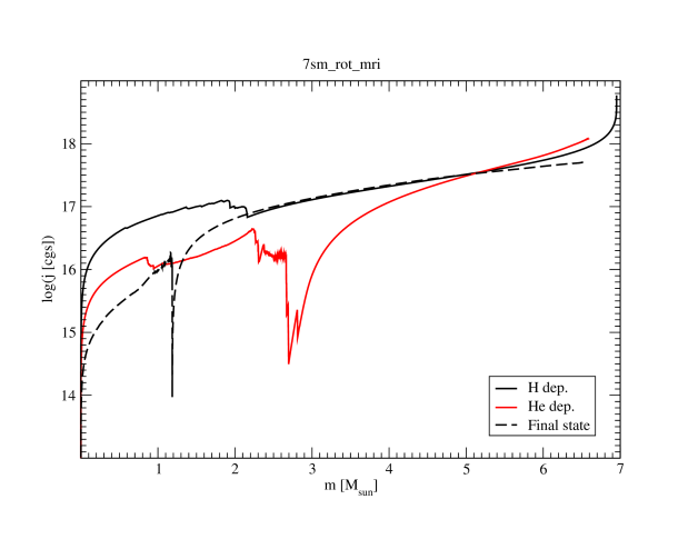
Figure 1.— Distribution with respect to mass of the specific angular momentum in the model with ZAMS mass of 7 M_⊙ at the end of hydrogen burning, at the end of helium burning, and in the final model with a degenerate O/Ne core for the model with MRI, but not ST, active. See the online version for color.

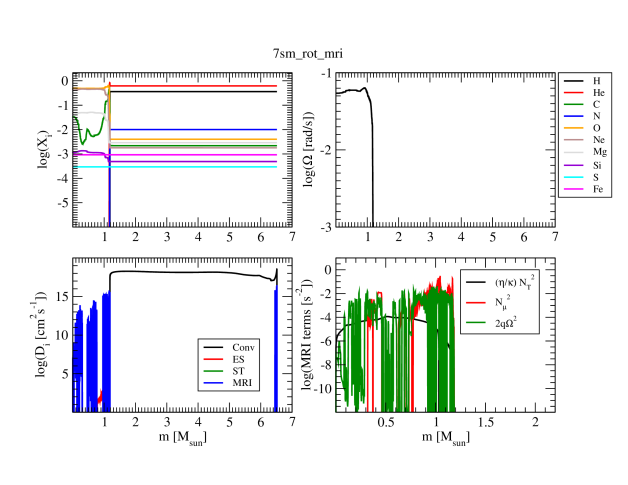
Figure 2.— Distribution with respect to mass in the final model of ZAMS mass of 7 M_⊙ of the composition (upper left), the angular velocity, $\Omega$ (upper right), the components of the diffusion coefficient (lower left), and the components of the MRI instability criterion (lower right) for the model with MRI, but not ST, active. See the online version for color.

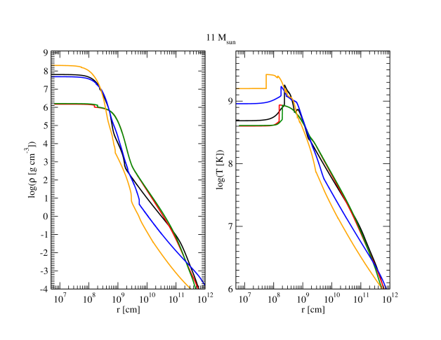
Figure 3.— Radial distributions of density and temperature for the “final" models corresponding to ZAMS mass of 11 M_⊙ for the cases with no rotation (black), rotation but no magnetic effects (red), ST but not MRI (green), MRI but not ST (blue), and with both ST and MRI active (orange). These models were halted artificially, see text. See the online version for color.

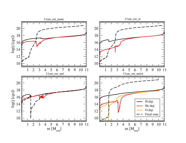
Figure 4.— Distribution with respect to mass in the models with ZAMS mass of 11 M_⊙ of the specific angular momentum at the end of hydrogen burning (black solid line), helium burning (red line), oxygen burning (orange line), and for the “final" model (black dashed line) for the cases with rotation but no magnetic effects (upper left), ST but not MRI (upper right), MRI but not ST (lower left), and with both ST and MRI active (lower left). These models were halted artificially, see text. None reached core collapse and only the model with both ST and MRI active completed oxygen burning. See the online version for color.

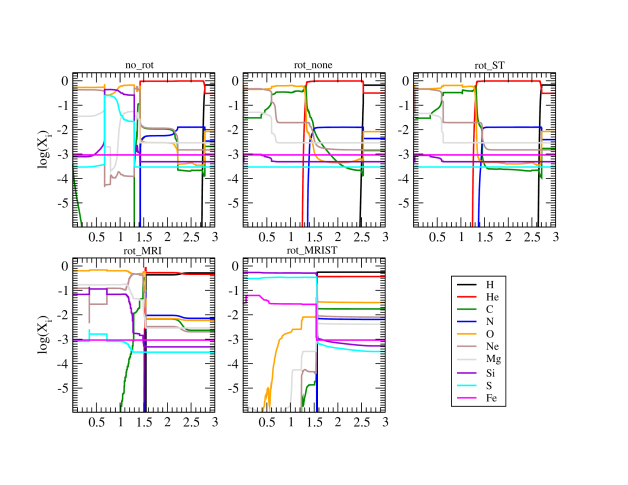
Figure 5.— Distribution with respect to mass in the model with ZAMS mass of 11 M_⊙ of the “final" composition of the various models of Figure 3. See the online version for color.

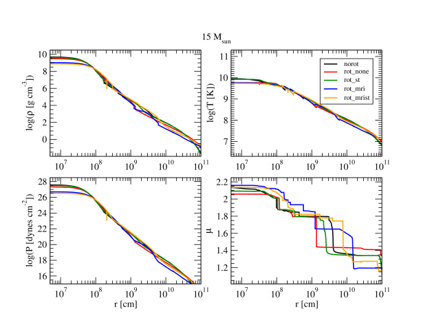
Figure 6.— Radial distributions of density (upper left), temperature (upper right), pressure (lower left) and mean molecular weight (lower right) for the final model corresponding to the fiducial model with ZAMS mass of 15 M_⊙ for the cases with no rotation, rotation but no magnetic effects, ST but not MRI, MRI but not ST, and with both ST and MRI active. See the online version for color.

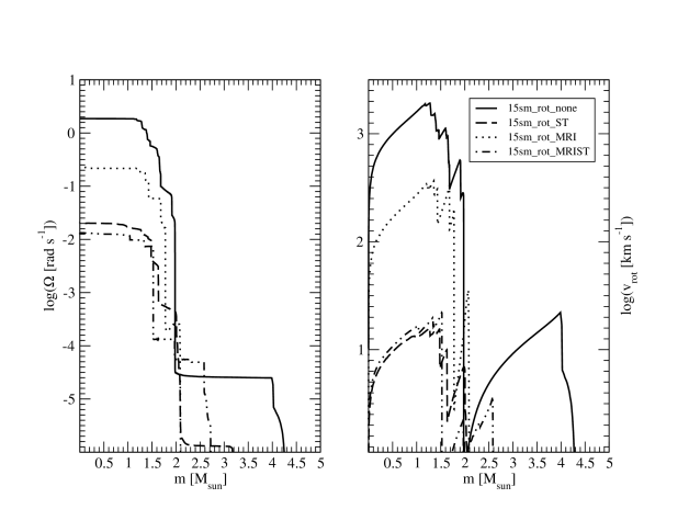
Figure 7.— Distributions of angular velocity (left) and rotation velocity on the equator (right) at the end of the calculation of the fiducial rotating model of ZAMS mass of 15 M_⊙ for the cases with no magnetic effects (solid line), ST only (dashed line), MRI only (dotted line), and with both ST and MRI active (dot–dash line).

Figure 8.— Distribution with respect to mass of the magnetic field at the end of the calculation, just prior to core collapse, of the fiducial rotating model of 15 M_⊙. Top, the case where the ST, but not MRI, is active; bottom, the case where the MRI, but not ST, is active. Both the toroidal (red) and radial (black) fields are presented. For the ST mechanism, the radial field is much less than the toroidal field, leading to a relatively small magnetic viscosity. For the MRI, the radial field is a constant fraction, 0.32, of the toroidal field. Note that while sparsely distributed, the strength of the toroidal field in the case of the MRI far exceeds that of the ST mechanism. The relatively large radial field contributes to a larger magnetic viscosity in the case of the MRI. See the online version for color.

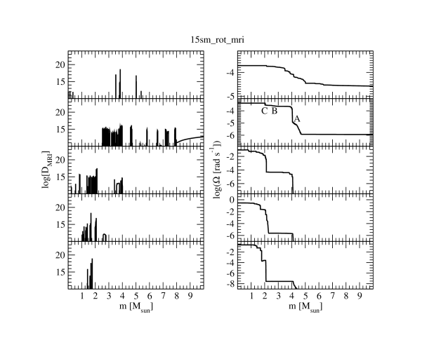
Figure 9.— Distribution with respect to mass of the MRI diffusion coefficient (left) and angular velocity (right) at the end of hydrogen burning, helium burning, oxygen burning, silicon burning, and at the onset of core collapse (top to bottom) for the fiducial model of ZAMS mass 15 M_⊙ for the rotating model with the MRI, but not ST, active. For panel 2 on the right, locations A, B, and C denote regions of steep or shallow gradients in $\Omega$ where shear generates MRI at the end of core helium burning (see Figure 10).

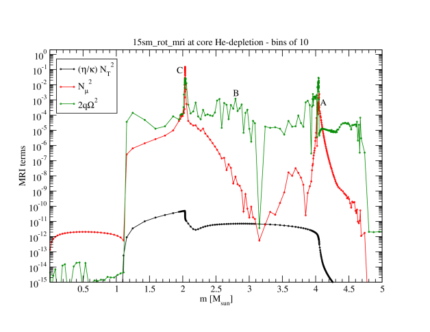
Figure 10.— Distribution with respect to mass of the terms that contribute to the instability criterion of the MRI at the end of core helium burning of the fiducial rotating model of ZAMS mass 15 M_⊙ for the case where the MRI, but not ST, is active. The terms are $(\eta/\kappa)N_{T}^{2}$ (black), $N_{\mu}^{2}$ (red), and $2q\Omega^{2}$ (green), where the latter is the driving term for the MRI. Locations A and B denote regions of steep or shallow gradients in $\Omega$ where shear generates MRI (see Figure 9). The small step in $\Omega$ and hence shear at point C at 2.03 M_⊙ in Figure 9 is stabilized by the composition buoyancy there, but regions on either side are unstable. See the online version for color.

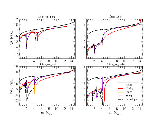
Figure 11.— Distribution with respect to mass in the fiducial model with ZAMS mass of 15 M_⊙ of the specific angular momentum at the end of hydrogen burning, helium burning, oxygen burning, silicon burning, and at the onset of core collapse for the cases with rotation but no magnetic effects (upper left), ST but not MRI (upper right), MRI but not ST (lower left), and with both ST and MRI active (lower right). See the online version for color.

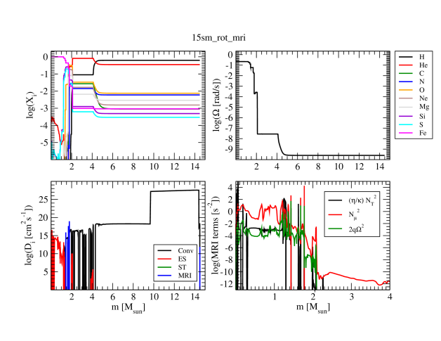
Figure 12.— Distribution with respect to mass in the model with ZAMS mass of 15 M_⊙ of the final distributions of composition (upper left), angular velocity (upper right), diffusion coefficients (lower left) and the components of the MRI instability criterion (lower right) for the model with the MRI, but not ST, active. See the online version for color.

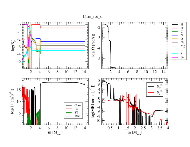
Figure 13.— Distribution with respect to mass in the model with ZAMS mass of 15 M_⊙ of the final distributions of composition (upper left), angular velocity (upper right), diffusion coefficients (lower left) and the thermal and composition components of the Brunt–Väisälä frequency (lower right) for the model with the ST, but not MRI, active. See the online version for color.

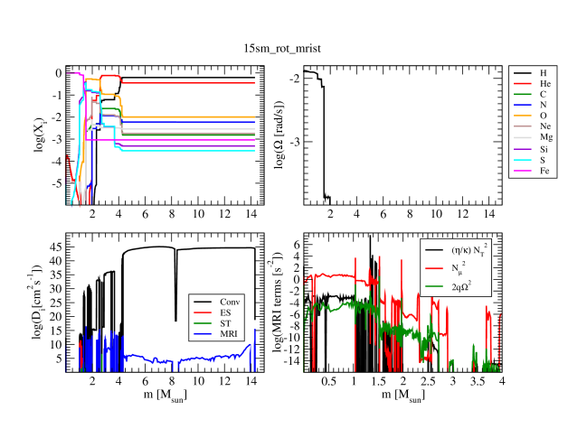
Figure 14.— Distribution with respect to mass in the model with ZAMS mass of 15 M_⊙ of the final distributions of composition (upper left), angular velocity (upper right), diffusion coefficients (lower left) and the components of the MRI instability criterion (lower right) for the model with both ST and MRI active. See the online version for color.

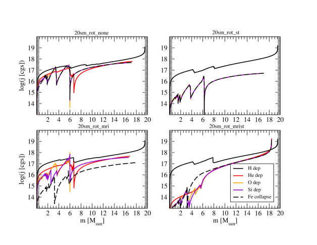
Figure 15.— Distribution with respect to mass in the model with ZAMS mass of 20 M_⊙ of the angular momentum per unit mass at the end of hydrogen burning, helium burning, oxygen burning, silicon burning, and at the onset of core collapse for the cases with rotation but no magnetic effects (upper left), ST but not MRI (upper right), MRI but not ST (lower left), and with both ST and MRI active (lower right). See the online version for color.

Figure 16.— Distributions of angular velocity (left) and rotation velocity on the equator (right) at the end of the calculation of the rotating model of 20 M_⊙ for the cases with no magnetic effects (solid line), ST but no MRI (dashed line), MRI but no ST (dotted line), and with both ST and MRI active (dot–dash line).

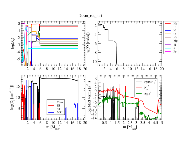
Figure 17.— Distribution with respect to mass in the model with ZAMS mass of 20 M_⊙ of the final distributions of composition (upper left), angular velocity (upper right), diffusion coefficients (lower right) and the components of the MRI instability criterion (lower right) for the model with the MRI, but not ST, active. See the online version for color.

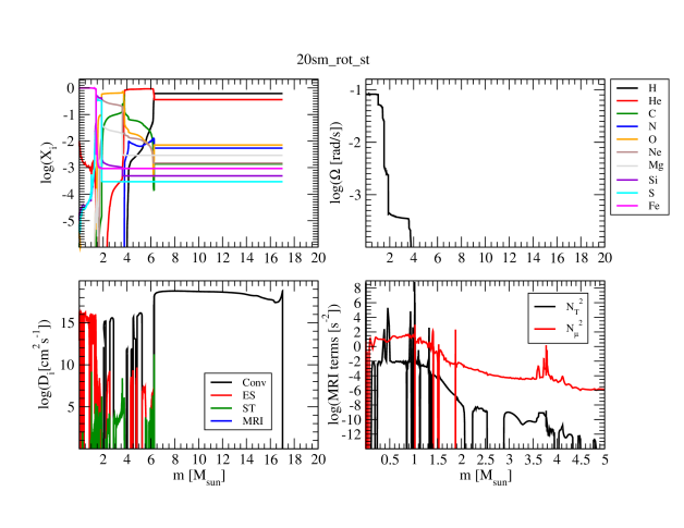
Figure 18.— Distribution with respect to mass in the model with ZAMS mass of 20 M_⊙ of the final distributions of composition (upper left), angular velocity (upper right), diffusion coefficients (lower right) and the thermal and composition components of the Brunt–Väisälä frequency (lower right) for the model with ST, but not MRI, active. See the online version for color.

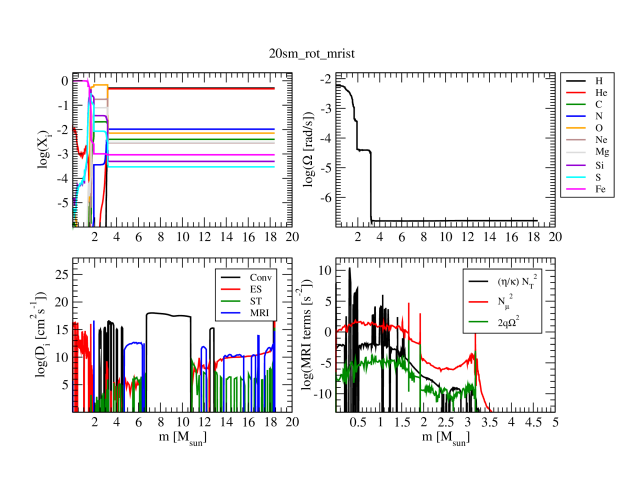
Figure 19.— Distribution with respect to mass in the model with ZAMS mass of 20 M_⊙ of the final distributions of composition (upper left), angular velocity (upper right), diffusion coefficients (lower right) and the components of the MRI instability criterion (lower right) for the model with both ST and MRI active. See the online version for color.

References

- Akiyama et al. (2003) Akiyama, S., Wheeler, J. C., Meier, D. L., & Lichtenstadt, I. 2003, Ap. J., 584, 954
- Acheson (1978) Acheson, D. J. 1978, Royal Society of London Philosophical Transactions Series A, 289, 459
- Armitage (2011) Armitage, P. J. 2011, ARA&A, 49, 195
- Arnett & Meakin (2011) Arnett, W. D., & Meakin, C. 2011, Ap. J., 733, 78
- Balbus & Hawley (1991) Balbus, S. A. & Hawley, J. F. 1991, Ap. J., 376, 214
- Balbus & Hawley (1994) Balbus, S. A., & Hawley, J. F. 1994, Mon. Not. Royal. Soc., 266, 769
- Balbus & Hawley (1998) Balbus, S. A. & Hawley, J. F. 1998, Review of Modern Physics, 70, 1
- Bellan (2006) Bellan, P. M. 2006, Fundamentals of Plasma Physics, Cambridge, UK: Cambridge University Press
- Blondin et al. (2003) Blondin, J. M., Mezzacappa, A., & DeMarino, C. 2003, Ap. J., 584, 971
- Blondin & Mezzacappa (2007) Blondin, J. M., & Mezzacappa, A. 2007, Nature, 445, 58
- Braithwaite (2006) Braithwaite, J. 2006, Astron. & Astroph., 449, 451
- Braithwaite (2009) Braithwaite, J. 2009, Mon. Not. Royal. Soc., 397, 763
- Brott et al. (2011) Brott, I., de Mink, S. E., Cantiello, M., et al. 2011, Astron. & Astroph., 530, A115
- Brun et al. (2005) Brun, A. S., Browning, M. K., & Toomre, J. 2005, Ap. J., 629, 461
- Burrows et al. (2007) Burrows, A., Dessart, L., Livne, E., Ott, C. D., & Murphy, J. 2007, Ap. J., 664, 416
- Cantiello et al. (2007) Cantiello, M., Yoon, S.-C., Langer, N., & Livio, M. 2007, Astron. & Astroph., 465, L29
- Cantiello et al. (2014) Cantiello, M., Mankovich, C., Bildsten, L., Christensen-Dalsgaard, J., & Paxton, B. 2014, Ap. J., 788, 93
- Chandrasekhar (1960) Chandrasekhar, S. 1960, Proc. Nat. Acad. Sci., 46, 253
- Chatzopoulos & Wheeler (2012) Chatzopoulos, E., & Wheeler, J. C. 2012, Ap. J., 748, 42
- Christensen-Dalsgaard et al. (1996) Christensen-Dalsgaard, J., et al. 1996, Science, 272, 1286
- Couch & Ott (2013) Couch, S. M., & Ott, C. D. 2013, Ap. J. Lett., 778, L7
- Davis et al. (2010) Davis, S. W., Stone, J. M., & Pessah, M. E. 2010, Ap. J., 713, 52
- Denissenkov & Pinsonneault (2007) Denissenkov, P. A., & Pinsonneault, M. 2007, Ap. J., 655, 1157
- Denissenkov (2010) Denissenkov, P. A. 2010, Ap. J., 723, 563
- de Jager et al. (1988) de Jager, C., Nieuwenhuijzen, H., & van der Hucht, K. A. 1988, A&AS, 72, 259
- Duncan & Thompson (1992) Duncan, R. C., & Thompson, C. 1992, Ap. J. Lett., 392, L9
- Endal & Sofia (1981) Endal, A. S., & Sofia, S. 1981, Ap. J., 243, 625
- Ekström et al. (2012) Ekström, S., Georgy, C., Eggenberger, P., et al. 2012, Astron. & Astroph., 537, A146
- Fricke (1969) Fricke, K. 1969, Astrophys. Lett., 3, 219
- Goldreich & Schubert (1967) Goldreich, P., & Schubert, G. 1967, Ap. J., 150, 571
- Hawley et al. (2011) Hawley, J. F., Guan, X., & Krolik, J. H. 2011, Ap. J., 738, 84
- Hawley et al. (2013) Hawley, J. F., Richers, S. A., Guan, X., & Krolik, J. H. 2013, Ap. J., 772, 102
- Heger et al. (2000) Heger, A., Langer, N., & Woosley, S. E. 2000, Ap. J., 528, 368
- Heger et al. (2005) Heger, A., Woosley, S. E., & Spruit, H. C. 2005, Ap. J., 626, 350
- Howe (2009) Howe, R. 2009, Living Reviews in Solar Physics, 6, 1
- Johansen et al. (2006) Johansen, A., Klahr, H., & Mee, A. J. 2006, Mon. Not. Royal. Soc., 370, L71
- Kagan & Wheeler (2014) Kagan, D., & Wheeler, J. C. 2014, Ap. J., 787, 21
- Kulsrud (2005) Kulsrud, R. M. 2005, Plasma Physics for Astrophysics Princeton, N.J. : Princeton University Press
- Maeder (2009) Maeder, A. 2009, Physics, Formation and Evolution of Rotating Stars (Springer Berlin Heidelberg)
- Maeder & Meynet (2004) Maeder, A., & Meynet, G. 2004, Astron. & Astroph., 422, 225
- Maeder & Meynet (2005) Maeder, A., & Meynet, G. 2005, Astron. & Astroph., 440, 1041
- Maeder & Meynet (2014) Maeder, A., & Meynet, G. 2014, Rev. Mod. Phys. in press (arXiv:1109.6171)
- Masada (2011) Masada, Y. 2011, Mon. Not. Royal. Soc., 411, L26
- Masada et al. (2006) Masada, Y., Sano, T., Takabe, H. 2006, Ap. J., 641, 447
- Masada et al. (2007) Masada, Y., Sano, T., Shibata, K. 2007, Ap. J., 655, 447
- Mazzali et al. (2014) Mazzali, P., MacFadyen, A., Woosley, S., Pian, E., & Tanaka, M. 2014, Mon. Not. Royal. Soc., in press
- Menou et al. (2004) Menou, K., Balbus, S. A., & Spruit, H. C. 2004, Ap. J., 607, 564
- Mitchell et al. (2013) Mitchell, J. P., Braithwaite, J., Langer, N., Reisenegger, A., & Spruit, H. 2014, Proceedings of IAUS 302: “Magnetic Fields Throughout Stellar Evolution," (arXiv:1310.2595)
- Miyaji et al. (1980) Miyaji, S., Nomoto, K., Yokoi, K., & Sugimoto, D. 1980, PASJ, 32, 303
- Mocák et al. (2011) Mocák, M., Meakin, C. A., Müller, E., & Siess, L. 2011, Ap. J., 743, 55
- Mösta et al. (2014) Mösta, P., Richers, S., Ott, C. D., et al. 2014, Ap. J. Lett., 785, L29
- Obergaulinger et al. (2009) Obergaulinger, M., Cerdá-Durán, P., Müller, E., & Aloy, M. A. 2009, Astron. & Astroph., 498, 241
- O’Connor & Ott (2011) O’Connor, E., & Ott, C. D. 2011, Ap. J., 730, 70
- Parfrey & Menou (2007) Parfrey, K. P., & Menou, K. 2007, Ap. J. Lett., 667, L207
- Paxton et al. (2011) Paxton, B., Bildsten, L., Dotter, A., et al. 2011, Ap. J. Supp., 192, 3
- Paxton et al. (2013) Paxton, B., Cantiello, M., Arras, P., et al. 2013, arXiv:1301.0319
- Petrovic et al. (2005) Petrovic, J., Langer, N., & van der Hucht, K. A. 2005, Astron. & Astroph., 435, 1013
- Pino & Mahajan (2008) Pino, J., & Mahajan, S. M. 2008, Ap. J., 678, 1223
- Pino & Mahajan (2009) Pino, J., & Mahajan, S. M. 2009, Ap. J., 697, 1805
- Sawai & Yamada (2014) Sawai, H., & Yamada, S. 2014, Ap. J. Lett., arXiv:1402.0513
- Shi et al. (2010) Shi, J., Krolik, J. H., & Hirose, S. 2010, Ap. J., 708, 1716
- Smartt (2009) Smartt, S. J. 2009, ARA&A, 47, 63
- Spitzer (2006) Spitzer, L. Jr. 2006, The Physics of Fully Ionized Gases, New York: Dover
- Spruit (1999) Spruit, H. C. 1999, Astron. & Astroph., 349, 189
- Spruit (2002) Spruit, H. C. 2002, Astron. & Astroph., 381, 923
- Suijs et al. (2008) Suijs, M. P. L., Langer, N., Poelarends, A.-J., Yoon, S.-C., Heger, A., & Herwig, F. 2008, Astron. & Astroph., 481, L87
- Tassoul (1978) Tassoul, J.-L. 1978, Princeton Series in Physics, Princeton: University Press
- Tayler (1973) Tayler, R. J. 1973, Mon. Not. Royal. Soc., 161, 365
- Timmes (1999) Timmes, F. X. 1999, Ap. J. Supp., 124, 241
- Timmes & Swesty (2000) Timmes, F. X., & Swesty, F. D. 2000, Ap. J. Supp., 126, 501
- Ugliano et al. (2012) Ugliano, M., Janka, H.-T., Marek, A., & Arcones, A. 2012, Ap. J., 757, 69
- Velikhov (1950) Velikhov, E. P. 1959, J. Exp. Theoret. Phys. (USSR), 36, 1398
- Vink et al. (2001) Vink, J. S., de Koter, A., & Lamers, H. J. G. L. M. 2001, Astron. & Astroph., 369, 574
- Vishniac (2009) Vishniac, E. T. 2009, Ap. J., 696, 1021
- Von Zeipel (1924) Von Zeipel, H. 1924, in Probleme der Astronomie, Festschrift für H. v. Seeliger, ed H. Kienle, (Springer, Berlin), p. 144
- Woosley (1993) Woosley, S. E. 1993, Ap. J., 405, 273
- Yoon et al. (2010) Yoon, S.-C., Woosley, S. E., & Langer, N. 2010, Ap. J., 725, 940
- Yoon et al. (2012) Yoon, S.-C., Dierks, A., & Langer, N. 2012, Astron. & Astroph., 542, A113
- Zahn et al. (2007) Zahn, J.-P., Brun, A. S., & Mathis, S. 2007, Astron. & Astroph., 474, 145