Computing minimal interpolants in $C^{1,1}(\mathbb{R}^{d})$

Abstract

We consider the following interpolation problem. Suppose one is given a finite set $E\subset\mathbb{R}^{d}$, a function $f:E\rightarrow\mathbb{R}$, and possibly the gradients of $f$ at the points of $E$. We want to interpolate the given information with a function $F\in C^{1,1}(\mathbb{R}^{d})$ with the minimum possible value of $\mathrm{Lip}(\nabla F)$. We present practical, efficient algorithms for constructing an $F$ such that $\mathrm{Lip}(\nabla F)$ is minimal, or for less computational effort, within a small dimensionless constant of being minimal.

October 24, 2016

arXiv:1411.5668

1 Introduction

We consider the problem of computing interpolants in $C^{1,1}(\mathbb{R}^{d})$, that is the space of functions whose derivatives are Lipschitz:

$$C^{1,1}(\mathbb{R}^{d}) =\{g:\mathbb{R}^{d}\rightarrow\mathbb{R}\mid\mathrm{Lip}(\nabla g)<\infty\},$$

$$\mathrm{Lip}(\nabla g) =\sup_{\begin{subarray}{c}x,y\in\mathbb{R}^{d}\\ x\neq y\end{subarray}}\frac{|\nabla g(x)-\nabla g(y)|}{|x-y|},$$

where $|\cdot|$ denotes the Euclidean norm. Analogous to interpolation by Lipschitz functions, in which one wishes to minimize the Lipschitz constant of the interpolant, here we aim to minimize the Lipschitz constant of the gradient of the interpolant. We consider two closely related problems, the first of which is the following:

Jet interpolation problem: One is given a finite set of points $E\subset\mathbb{R}^{d}$, and at each point $a\in E$, a function value $f_{a}\in\mathbb{R}$ and a gradient $D_{a}f\in\mathbb{R}^{d}$ are specified. Compute an interpolating function $F\in C^{1,1}(\mathbb{R}^{d})$ such that:

1. $F(a)=f_{a}$ and $\nabla F(a)=D_{a}f$ for each $a\in E$.

2. Amongst all such interpolants satisfying the previous condition, the value of $\mathrm{Lip}(\nabla F)$ is minimal.
   

The Jet interpolation problem is a computational version of Whitney’s Extension Theorem [41]. Whitney’s Extension Theorem is a partial converse to Taylor’s Theorem. Given a closed set $E\subset\mathbb{R}^{d}$ (not necessarily finite) and an $m^{\text{th}}$ degree polynomial at each point of $E$, Whitney’s Extension Theorem states that if the collection of polynomials satisfies certain compatibility conditions, then there exists a function $F\in C^{m}(\mathbb{R}^{d})$ such that for each point $a\in E$ the $m^{\text{th}}$ order Taylor expansion of $F$ at $a$ agrees with the polynomial specified at that point. A similar result can be stated for $C^{m-1,1}(\mathbb{R}^{d})$ with $(m-1)^{\text{st}}$ degree polynomials given at each point of $E$. In the case of $C^{1,1}(\mathbb{R}^{d})$, the polynomials are defined by the specified function and gradient information:

$$P_{a}(x)=f_{a}+D_{a}f\cdot(x-a),\quad a\in E,\enspace x\in\mathbb{R}^{d}.$$

Letting $\mathcal{P}$ denote the space of first order polynomials, the map

$$P:\mathbb{R}^{d} \rightarrow\mathcal{P},$$

$$a \mapsto P_{a},$$

is called a 1-field (or a Whitney field). For a function $F\in C^{1,1}(\mathbb{R}^{d})$, the first order Taylor expansions of $F$ are elements of $\mathcal{P}$. Such expansions are called jets, and are defined as:

$$J_{a}F(x)=F(a)+\nabla F(a)\cdot(x-a),\quad a,x\in\mathbb{R}^{d}.$$

Whitney’s Extension Theorem for $C^{1,1}(\mathbb{R}^{d})$ can then be stated as follows.

Theorem 1.1 (Whitney’s Extension Theorem for $C^{1,1}(\mathbb{R}^{d})$).

Let $E\subset\mathbb{R}^{d}$ be closed and let $P:E\rightarrow\mathcal{P}$ be a 1-field with domain $E$. If there exists a constant $M<\infty$ such that

1. $|P_{a}(a)-P_{b}(a)|\leq M|a-b|^{2}$, for all $a,b\in E$,

2. $|\frac{\partial P_{a}}{\partial x_{i}}(a)-\frac{\partial P_{b}}{\partial x_{i}}(a)|\leq M|a-b|$, for all $a,b\in E$ and $i=1,\ldots,d$,

then there exists an extension $F\in C^{1,1}(\mathbb{R}^{d})$ such that $J_{a}F=P_{a}$ for all $a\in E$.

When the set $E$ is finite, the compatibility conditions of Whitney’s Extension Theorem are automatically satisfied. On the other hand, the theorem cannot be used to derive the minimal value of $\mathrm{Lip}(\nabla F)$. Denote this value as:

$$\|P\|_{C^{1,1}(E)}=\inf\{\mathrm{Lip}(\nabla\widetilde{F})\mid J_{a}\widetilde{F}=P_{a}\text{ for all }a\in E\}.$$

Indeed, if one were to take the infimum over all possible $M$ satisfying $(W_{0})$ and $(W_{1})$, the resulting value would only be within a constant $C(d)$ of $\|P\|_{C^{1,1}(E)}$. A recent paper by Le Gruyer [33] solves this problem in closed form by defining a functional $\Gamma^{1}$ such that $\Gamma^{1}(P;E)=\|P\|_{C^{1,1}(E)}$. This is the first ingredient in our solution to the Jet interpolation problem. The second is a result of Wells [40], which gives a construction of an interpolant $F\in C^{1,1}(\mathbb{R}^{d})$ with $\mathrm{Lip}(\nabla F)=M$ for a specified value of $M$ satisfying certain conditions. It is easy to show that $M=\Gamma^{1}(P;E)$ satisfies the conditions, and thus one can combine the two results to obtain a minimal interpolant. The construction of Wells is not simple, however, and must be adapted to certain data structures implementable on a computer. Thus our third ingredient is a collection of algorithms and data structures from computational geometry that compute and encode the results of Le Gruyer and Wells.

The second problem we consider is when only the function values are specified:

Function interpolation problem: One is given a finite set of points $E\subset\mathbb{R}^{d}$ and a function $f:E\rightarrow\mathbb{R}$. Compute an interpolating function $F\in C^{1,1}(\mathbb{R}^{d})$ such that:

1. $F(a)=f(a)$ for each $a\in E$.

2. Amongst all such interpolants satisfying the previous condition, the value of $\mathrm{Lip}(\nabla F)$ is minimal.
   

The Function interpolation problem is harder than the Jet interpolation problem since the space of functions satisfying $F(a)=f(a)$ is larger than the space of functions satisfying $J_{a}F=P_{a}$. However, the minimal value of $\mathrm{Lip}(\nabla F)$ can be specified using the functional $\Gamma^{1}$. Indeed, let $\|f\|_{C^{1,1}(E)}$ denote the minimal value of $\mathrm{Lip}(\nabla F)$, where

$$\|f\|_{C^{1,1}(E)}=\inf\{\mathrm{Lip}(\nabla\widetilde{F})\mid\widetilde{F}(a)=f(a)\text{ for all }a\in E\}.$$

For functions $f$, define the $\Gamma^{1}$ functional as:

$$\Gamma^{1}(f;E)=\inf\{\Gamma^{1}(P;E)\mid P_{a}(a)=f(a)\text{ for all }a\in E\}.$$

Then, as is shown in [33], $\Gamma^{1}(f;E)=\|f\|_{C^{1,1}(E)}$. The functional $\Gamma^{1}$ is convex, and thus $\Gamma^{1}(f;E)$ can be computed using convex programming. Additionally, the minimizing 1-field can be outputted. Then one can use the remainder of the Jet interpolation problem algorithm to solve the Function interpolation problem.

The purpose of this paper is twofold, with one aspect being the theoretical efficiency of our algorithms, but the other, equally important aspect, being the practicality of our algorithms. Indeed, the goal is to balance the two; sometimes this results in trading theoretical efficiency for algorithms that can be implemented and run a computer, while in other cases we prove new theoretical results that are of practical interest.

On the theoretical side, we assume that our computer is able to work with exact real numbers. We ignore roundoff, overflow, and underflow errors, and suppose that an exact real number can be stored at each memory address. Additionally, we suppose that it takes one machine operation to add, subtract, multiply, or divide two real numbers $x$ and $y$, or to compare them (i.e., decide whether $x<y$, $x>y$, or $x=y$).

From a more practical perspective, we do not always implement algorithms with optimal theoretical worst case guarantees in terms of complexity, opting to choose an alternative that works better in practice. Additionally, at various stages of our interpolation algorithm we may give multiple options for computing the next step. The difference between the options might depend on $N$ and $d$, or one might be more stable than another in certain situations. In Section 7 we give a summary of numerical simulations of the algorithm running on a computer.

The work of an algorithm is the number of machine operations needed to carry it out, and the storage of an algorithm is the number of random access memory addresses required.

In order to analyze the complexity of the algorithm, we break it into three main components: the aforementioned storage, the one time work, and the query work. The one time work consists of the following: given the set $E$ and either the 1-field $P$ or the function $f$, the algorithm performs a certain amount of preprocessing, after which it is ready to accept queries from the user. The number of computations needed for this preprocessing stage is the one time work. The algorithm additionally outputs $\mathrm{Lip}(\nabla F)$ at the end of this stage. Once the one time work is complete, the user inputs a query point $x\in\mathbb{R}^{d}$, and the algorithm returns $J_{x}F$ (i.e. $F(x)$ along with $\nabla F(x)$). The amount of work for each query is the query work.

Recently, there has been an interest in algorithmic results related to Whitney’s Extension Theorem. One can recast the Function interpolation problem in terms of interpolants $F\in C^{m}(\mathbb{R}^{d})$, with the goal to minimize an appropriate $C^{m}$ norm. Suppose that $\#(E)=N$. In [21], an algorithm is presented which computes a number $M$ such that $M$ has the same order magnitude as $\|f\|_{C^{m}(E)}$, that is $c(m,d)M\leq\|f\|_{C^{m}(E)}\leq C(m,d)M$. The algorithm requires $O(N\log N)$ work and $O(N)$ storage. In a second, companion paper [22], an additional algorithm is presented which computes a function $F\in C^{m}(\mathbb{R}^{d})$ such that $F$ interpolates the given function and $c(m,d)\|F\|_{C^{m}(\mathbb{R}^{d})}\leq\|f\|_{C^{m}(E)}\leq C(m,d)\|F\|_{C^{m}(\mathbb{R}^{d})}$. The one time work of the algorithm requires $O(N\log N)$ operations, the query work requires $O(\log N)$ operations, and the storage never exceeds $O(N)$. Analogous results describing a new algorithm for fitting a Sobolev function to data are presented in [20].

In related work [19], the task of computing an $F$ such that $\|F\|_{C^{m}(\mathbb{R}^{d})}$ is within a factor of $1+\epsilon$ of $\|f\|_{C^{m}(E)}$ is considered. A linear programming problem is devised which solves the problem. The number of linear constraints grows linearly in $N$ and as $O(\epsilon^{-\frac{3}{2}d})$ in $\epsilon$.

In terms of the efficiency with regards to $N$, these algorithms are optimal. However, the dimension dependent constants can grow exponentially with $d$. Additionally, while the algorithms are beautiful, they are also intricate. Thus, from a practical perspective, they are not likely to be implemented on a computer and used in applications.

Our algorithm, while not always reaching the optimal theoretical complexity guarantees of the previously mentioned algorithms, is to the best of our knowledge the first of its type to be implemented on a computer and be practical for certain tasks. The key features of our $C^{1,1}$ algorithm are:

• We can compute $\|P\|_{C^{1,1}(E)}$ precisely in $O(N^{2})$ work, or to within a dimensionless constant (approximately $20$) of $\|P\|_{C^{1,1}(E)}$ using $O(N\log N)$ work.

• We can compute $\|f\|_{C^{1,1}(E)}$ to within a dimensionless constant (again approximately $20$) plus an arbitrarily small additive slack $\epsilon$ using interior point methods from convex optimization. The number of iterations is sublinear, $O((N\log N)^{1/2}\log(N/\epsilon))$, and the cost per iteration is $O(N^{3})$, although sparsity considerations may improve this computational time in practice.

• For the one time work outside of computing $\|P\|_{C^{1,1}(E)}$ or $\|f\|_{C^{1,1}(E)}$, the efficiency of the algorithm is tied to the complexity of computing and storing a convex hull. Computing a convex hull requires $O(N\log N+N^{\lceil d/2\rceil})$ operations, and its storage is $O(N^{\lceil d/2\rceil})$. Subsequently, the work of our algorithm is $O(N^{d+2})$ and the storage is $O(N^{\lceil d/2\rceil+1})$.

• With some additional one time work and under suitable conditions, the query work requires only $O(\log N)$ operations.

• A version of the algorithm that runs from start to finish has been implemented in $\text{MATLAB}^{\circledR}$ and can be run on a laptop for small problems, and is practical on a server for larger problems. The complete code can be downloaded at:

  $$\href https://github.com/matthew-hirn/C-1-1-Interpolation$$

  The code is easy to use and not difficult to edit. Throughout the paper we highlight which parts of the algorithm have been implemented, and discuss the potential benefits of the parts that have not been implemented.

• The interpolant we compute is a generalized absolutely minimal Lipschitz extension (AMLE), as defined in [28].

Finally, the choice of the space $C^{1,1}(\mathbb{R}^{d})$ is natural in several ways beyond the existence of the results of Le Gruyer and Wells. Standard Lipschitz extensions in $C^{0,1}(\mathbb{R}^{d})$ and absolutely minimal Lipschitz extensions have applications in computer science [32], partial differential equations [7], and image processing [13], among others. The next non-trivial space to consider beyond $C^{0,1}(\mathbb{R}^{d})$ is $C^{1,1}(\mathbb{R}^{d})$. In fact, for $d=1$, the more general space $C^{m-1,1}(\mathbb{R})$ was originally considered by Favard [18] and later by Glaeser [24]. The solution $F$ of the Jet interpolation problem for this space is a spline $F\in C^{m-1,1}(\mathbb{R})$ made up of $C^{m}$-smooth pieces with at most $m-1$ knots. In cubic spline interpolation the spline either minimizes the integral of the curvature $\kappa$ [25],

$$\int\kappa(x)\,dx=\int\frac{|F^{(2)}(x)|^{2}}{(1+F^{(1)}(x)^{2})^{5/2}}\,dx,$$

or a simpler energy [29] such as:

(1.1) $$\|F^{(2)}\|_{L^{2}(\mathbb{R})}^{2}=\int|F^{(2)}(x)|^{2}\,dx.$$

In the setting of $C^{m-1,1}(\mathbb{R})$, though, the optimal splines minimize the energy:

$$\mathrm{Lip}(F^{(m-1)})=\sup_{x\in\mathbb{R}}|F^{(m)}(x)|=\|F^{(m)}\|_{L^{\infty}(\mathbb{R})}.$$

In light of (1.1), we see that in the $C^{m-1,1}(\mathbb{R})$ setting we have replaced the $L^{2}$ energy with an $L^{\infty}$ energy. In $d$-dimensions, a similar identity holds for $C^{1,1}(\mathbb{R}^{d})$:

$$\mathrm{Lip}(\nabla F)=\sup_{x\in\mathbb{R}^{d}}\|\nabla^{2}F(x)\|_{\mathrm{op}},$$

where $\|\cdot\|_{\mathrm{op}}$ is the operator norm. The interpolants we compute are piecewise quadratic, and thus are $d$-dimensional analogues to the quadratic splines of Glaeser. The “knots” in higher dimensions correspond to $(d-1)$-dimensional facets (for example, line segments in $\mathbb{R}^{2}$), along which there is a discontinuity in the second order partial derivatives of $F$.

In the work of Glaeser as well as many cubic spline interpolating schemes, the ordering of the real line allows one to reduce the $N$ point interpolation problem to a two point interpolation problem. When one transitions to $\mathbb{R}^{d}$ and asks for $d$-dimensional interpolants, however, the lack of natural ordering is problematic. This is where the work of Wells and Le Gruyer come into play, giving us a roadmap to navigate the higher dimensional Euclidean space.

While we have not applied our algorithm on real data, it would seem that the algorithm could be useful for various applications. For example, it could be used to aid in the design of experiments in applied physics and chemistry. Suppose a scientist wants to conduct a costly experiment in which he must deposit a thin film of $\text{SiO}_{2}$ in a special tool that has plasma in it. The success of this experiment depends on several factors, such as the pressure in the chamber, the temperature of the substrate, the voltage of the plasma, and the ratios of the gases involved. He wants to find the optimal conditions for performing the experiment. He knows that the voltage is a smooth function of the other parameters, but it is difficult to measure. Consequently, he can only measure it for a few different combinations of initial conditions. He varies each parameter slightly while holding the others constant to find the rate of change of the voltage with respect to that parameter. Now he has data points (configurations of the parameters), function values (measured voltages), and partial derivatives. Using our interpolation algorithm, it is possible to compute a good estimate of the voltage for any configuration of the parameters and thereby determine the optimal conditions for the experiment.

The remainder of this paper is organized as follows. In Section 2 we give the relevant background information regarding the results of Wells and Le Gruyer, as well as the pertinent material from computational geometry. In Section 3 we present an overview of the algorithm, while in Sections 4, 5, and 6 we fill in the details. In particular, we describe efficient algorithms for computing $\Gamma^{1}$ in Section 4, the remainder of the one time work is detailed in Section 5, and in Section 6 we present algorithms for the query work. Section 7 describes numerical simulations of the algorithm and its resulting performance. Appendix A reviews some standard textbook concepts from convex optimization, which can be found in [11].

2 Background

In this section we review the results of Wells and Le Gruyer, and go over the relevant material from computational geometry.

2.1 Wells: Constructing the interpolant

In [40] Wells describes a construction of an interpolant $F\in C^{1,1}(\mathbb{R}^{d})$ with specified semi-norm $\mathrm{Lip}(\nabla F)=M$. Our algorithm will be based on this construction, which we review here.

The inputs are the set $E\subset\mathbb{R}^{d}$, the 1-field $P:E\rightarrow\mathcal{P}$, which consists of the specified function values $\{f_{a}\}_{a\in E}\subset\mathbb{R}$ and gradients $\{D_{a}f\}_{a\in E}\subset\mathbb{R}^{d}$, and the value $M$. In order for Wells’ construction to hold, the following condition must be satisfied:

(2.1) $$f_{b}\leq f_{a}+\frac{1}{2}(D_{a}f+D_{b}f)\cdot(b-a)+\frac{M}{4}|b-a|^{2}-\frac{1}{4M}|D_{a}f-D_{b}f|^{2},\enspace\forall\,a,b\in E.$$

For each point $a\in E$, define a shifted point $\tilde{a}$:

$$\tilde{a}=a-\frac{D_{a}f}{M},\quad a\in E.$$

Additionally, to each point $a\in E$ Wells associates a type of distance function $d_{a}:\mathbb{R}^{d}\rightarrow\mathbb{R}$ from $\mathbb{R}^{d}$ to that point:

(2.2) $$d_{a}(x)=f_{a}-\frac{1}{2M}|D_{a}f|^{2}+\frac{M}{4}|x-\tilde{a}|^{2},\quad a\in E,\enspace x\in\mathbb{R}^{d}.$$

For any subset $S\subset E$ define $d_{S}:\mathbb{R}^{d}\rightarrow\mathbb{R}$ as

$$d_{S}(x)=\min_{a\in S}d_{a}(x),\quad x\in\mathbb{R}^{d}.$$

Using the shifted points and the distance functions, Wells associates to every subset $S\subset E$ several new sets:

$$\widetilde{S} =\{\tilde{a}\mid a\in S\},$$

$$S_{H} =\text{the smallest affine space containing }\widetilde{S},$$

$$\widehat{S} =\text{the convex hull of }\widetilde{S},$$

$$S_{E} =\{x\in\mathbb{R}^{d}\mid d_{a}(x)=d_{b}(x),\enspace\forall\,a,b\in S\},$$

$$S_{\ast} =\{x\in\mathbb{R}^{d}\mid d_{a}(x)=d_{b}(x)\leq d_{c}(x),\enspace\forall\,a,b\in S,\enspace c\in E\},$$

$$S_{C} =S_{H}\cap S_{E}.$$

Wells also defines a set of special subsets $S\subset E$:

(2.3) $$\mathcal{K}=\{S\subset E\mid\exists\,x\in S_{\ast}\text{ such that }d_{S}(x)<d_{E\setminus S}(x)\}.$$

Note that when $S\in\mathcal{K}$, $S_{E}\neq\emptyset$, $\dim S_{E}+\dim S_{H}=d$, and $S_{H}\perp S_{E}$; therefore $S_{C}$ is a single point in $\mathbb{R}^{d}$. Using the subsets contained in $\mathcal{K}$, Wells defines a new collection of sets $\{T_{S}\}_{S\in\mathcal{K}}$,

(2.4) $$T_{S}=\frac{1}{2}(\widehat{S}+S_{\ast})=\left\{\frac{1}{2}(y+z)\mid y\in\widehat{S},\enspace z\in S_{\ast}\right\},\quad S\in\mathcal{K}.$$

The collection $\{T_{S}\}_{S\in\mathcal{K}}$ forms a covering of $\mathbb{R}^{d}$ in which the regions of overlap have Lebesgue measure zero. On each set $T_{S}$, Wells defines a function $F_{S}:T_{S}\rightarrow\mathbb{R}$, which is a local piece of the final interpolant:

$$F_{S}(x)=d_{S}(S_{C})+\frac{M}{2}\mathrm{dist}(x,S_{H})^{2}-\frac{M}{2}\mathrm{dist}(x,S_{E})^{2},\quad x\in T_{S},\enspace S\in\mathcal{K},$$

where for any two sets $U,V\subset\mathbb{R}^{d}$

$$\mathrm{dist}(U,V)=\inf_{\begin{subarray}{c}x\in U\\ y\in V\end{subarray}}|x-y|.$$

The final function $F:\mathbb{R}^{d}\rightarrow\mathbb{R}$ is defined as:

(2.5) $$F(x)=F_{S}(x),\quad\text{if }x\in T_{S}.$$

If $T_{S}\cap T_{S^{\prime}}\neq\emptyset$, then $F_{S}$ and $F_{S^{\prime}}$ as well as $\nabla F_{S}$ and $\nabla F_{S^{\prime}}$ agree on $T_{S}\cap T_{S^{\prime}}$, so $F$ is well defined and $F\in C^{1,1}(\mathbb{R}^{d})$. Additionally, the gradient of $F_{S}$ has a simple analytic form, given by:

$$\nabla F_{S}(x)=\frac{M}{2}(z-y),\quad x=\frac{1}{2}(y+z),\enspace y\in\widehat{S},\enspace z\in S_{\ast}.$$

Finally, the function $F$ interpolates the data and has the prescribed semi-norm:

Theorem 2.1 (Wells, [40, Section 4, Theorem 1]).

Given a finite set $E\subset\mathbb{R}^{d}$, a 1-field $P:E\rightarrow\mathcal{P}$, and a constant $M$ satisfying (2.1), the function $F:\mathbb{R}^{d}\rightarrow\mathbb{R}$ defined by (2.5) is in $C^{1,1}(\mathbb{R}^{d})$ and additionally:

1. $J_{a}F=P_{a}$ for all $a\in E$,

2. $\mathrm{Lip}(\nabla F)=M$.

2.2 Le Gruyer: The minimal value of $\mathrm{Lip}(\nabla F)$

While the result of Wells gives a construction for an interpolant with prescribed semi-norm $M$, it does not explicitly give the minimum possible value of $M$. Recall that this minimum value is defined for $1$-fields as:

$$\|P\|_{C^{1,1}(E)}=\inf\{\mathrm{Lip}(\nabla\widetilde{F})\mid J_{a}\widetilde{F}=P_{a}\text{ for all }a\in E\},$$

and for functions as:

$$\|f\|_{C^{1,1}(E)}=\inf\{\mathrm{Lip}(\nabla\widetilde{F})\mid\widetilde{F}(a)=f(a)\text{ for all }a\in E\}.$$

As in [33], define the functional $\Gamma^{1}$ as:

(2.6) $$\Gamma^{1}(P;E)=2\sup_{x\in\mathbb{R}^{d}}\max_{\begin{subarray}{c}a,b\in E\\ a\neq b\end{subarray}}\frac{|P_{a}(x)-P_{b}(x)|}{|a-x|^{2}+|b-x|^{2}}.$$

Recall that for functions we defined $\Gamma^{1}(f;E)$ as:

$$\Gamma^{1}(f;E)=\inf\{\Gamma^{1}(P;E)\mid P_{a}(a)=f(a)\text{ for all }a\in E\}.$$

The following two results show that $\Gamma^{1}$ is equivalent to $\|\cdot\|_{C^{1,1}(E)}$.

Theorem 2.2 (Le Gruyer, [33, Theorem 1.1]).

Given a set $E\subset\mathbb{R}^{d}$ and a 1-field $P:E\rightarrow\mathcal{P}$,

$$\Gamma^{1}(P;E)=\|P\|_{C^{1,1}(E)}.$$

Corollary 2.3 (Le Gruyer, [33, Theorem 3.2]).

Given a set $E\subset\mathbb{R}^{d}$ and a function $f:E\rightarrow\mathbb{R}$,

$$\Gamma^{1}(f;E)=\|f\|_{C^{1,1}(E)}.$$

The functional $\Gamma^{1}(P;E)$ has an alternate form which will prove to be more useful than (2.6) from a computational perspective. Define two additional functionals:

$$A(P;a,b) =\frac{|P_{a}(a)-P_{b}(a)+P_{a}(b)-P_{b}(b)|}{|a-b|^{2}},\quad a,b\in E$$

$$B(P;a,b) =\frac{|\nabla P_{a}(a)-\nabla P_{b}(a)|}{|a-b|}=\frac{|D_{a}f-D_{b}f|}{|a-b|},\quad a,b\in E.$$

Then one can show [33, Proposition 2.2]:

(2.7) $$\Gamma^{1}(P;E)=\max_{\begin{subarray}{c}a,b\in E\\ a\neq b\end{subarray}}\sqrt{A(P;a,b)^{2}+B(P;a,b)^{2}}+A(P;a,b).$$

This alternate form removes the supremum and reduces the work of computing $\Gamma^{1}(P;E)$ to $O(N^{2})$. Additionally, using (2.7) it is not hard to show that $M=\Gamma^{1}(P;E)$ satisfies the Wells condition (2.1). Thus combining Wells’ Theorem 2.1 and Le Gruyer’s Theorem 2.2 we arrive at a minimal interpolant for the Jet interpolation problem. One can utilize Corollary 2.3 and Theorem 2.1 to obtain a solution for the Function interpolation problem, assuming that when one solves for $\Gamma^{1}(f;E)$ the minimizing 1-field is outputted as well.

In fact, by a recent result contained in [26], the interpolant $F$ of Wells with $M=\Gamma^{1}(P;E)$ is a generalized absolutely minimal Lipschitz extension (AMLE) according to the definition presented in [28]. To understand this statement, first note that the interpolant $F$ defines a 1-field through its jets, namely:

$$P^{(F)}:\mathbb{R}^{d} \rightarrow\mathcal{P},$$

$$a \mapsto J_{a}F.$$

The functional $\Gamma^{1}$ can be thought of as the Lipschitz constant for 1-fields. Indeed, aside from the main result that $\Gamma^{1}$ is equal to the minimum value of $\mathrm{Lip}(\nabla\widetilde{F})$ as $\widetilde{F}$ ranges over all interpolants, one can show additionally that,

$$\Gamma^{1}(P^{(F)};\mathbb{R}^{d})=\Gamma^{1}(P;E).$$

Thus the 1-field $P^{(F)}$ extends $P$ while preserving $\Gamma^{1}$. Note that this is analogous to the standard Lipschitz extension problem between Hilbert spaces, for which it is known that any Lipschitz function mapping a subset of Hilbert space to another Hilbert space can be extended while preserving the Lipschitz constant [31]. For real valued Lipschitz extensions, the notion of an AMLE goes back to Aronsson [4, 5, 6] and has been studied extensively due to its relationship to partial differential equations [30], stochastic games [36], and applications in applied mathematics [3, 7, 13, 1]. An AMLE is the locally best Lipschitz extension. The formal definition can be extended to other functionals such as $\Gamma^{1}$, where in this case we say an extension $Q:\mathbb{R}^{d}\rightarrow\mathcal{P}$ of $P$ is an AMLE if

1. $\Gamma^{1}(Q;\mathbb{R}^{d})=\Gamma^{1}(P;E)$,

2. For every open subset $V\subset\mathbb{R}^{d}\setminus E$,

   $$\Gamma^{1}(Q;V)=\Gamma^{1}(Q;\partial V).$$

A result in [26] states that $P^{(F)}$ is an AMLE when $E$ is finite. Thus the interpolant that our algorithm computes is an AMLE for $C^{1,1}(\mathbb{R}^{d})$. Given the interest in classical AMLEs, having an algorithm to compute them in the $C^{1,1}(\mathbb{R}^{d})$ case has the potential to be of use in suitable applications.

2.3 Computational geometry

We now review the relevant material from computational geometry.

2.3.1 Well separated pairs decomposition

The following is relevant for computing approximations of $\Gamma^{1}$ when the number of points $N$ is large. The well separated pairs decomposition was first introduced by Callahan and Kosaraju in [12]; we shall make use of a modified version that was described in detail in [21].

First, let $U,V\subset\mathbb{R}^{d}$ and recall the definitions of the diameter of a set and the distance between two sets:

$$\mathrm{diam}(U)=\sup_{\begin{subarray}{c}x,y\in U\\ x\neq y\end{subarray}}|x-y|,\qquad\mathrm{dist}(U,V)=\inf_{\begin{subarray}{c}x\in U\\ y\in V\end{subarray}}|x-y|.$$

For $\varepsilon>0$, two sets $U,V\subset\mathbb{R}^{d}$ are $\varepsilon$-separated if

$$\max\{\mathrm{diam}(U),\mathrm{diam}(V)\}<\varepsilon\cdot\mathrm{dist}(U,V).$$

We follow the construction detailed by Fefferman and Klartag in [21]. Let $\mathcal{T}$ be a collection of subsets of $E$. For any $\Lambda\subset\mathcal{T}$, set

$$\cup\Lambda=\bigcup_{S\in\Lambda}S=\{x\mid x\in S\text{ for some }S\in\Lambda\}.$$

Let $\mathcal{W}$ be a set of pairs $(\Lambda_{1},\Lambda_{2})$ where $\Lambda_{1},\Lambda_{2}\subset\mathcal{T}$. For any $\varepsilon>0$, the pair $(\mathcal{T},\mathcal{W})$ is an $\varepsilon$-well separated pairs decomposition or $\varepsilon$-WSPD for short if the following properties hold:

1. $\bigcup_{(\Lambda_{1},\Lambda_{2})\in\mathcal{W}}\cup\Lambda_{1}\times\cup\Lambda_{2}=\{(x,y)\in E\times E\mid x\neq y\}$.

2. If $(\Lambda_{1},\Lambda_{2}),(\Lambda_{1}^{\prime},\Lambda_{2}^{\prime})\in\mathcal{W}$ are distinct pairs, then $(\cup\Lambda_{1}\times\cup\Lambda_{2})\cap(\cup\Lambda_{1}^{\prime}\times\cup\Lambda_{2}^{\prime})=\emptyset$.

3. $\cup\Lambda_{1}$ and $\cup\Lambda_{2}$ are $\varepsilon$-separated for any $(\Lambda_{1},\Lambda_{2})\in\mathcal{W}$.

4. $\#(\mathcal{T})<C(\varepsilon,d)N$ and $\#(\mathcal{W})<C(\varepsilon,d)N$.

As shown in [21], there is a data structure representing $(\mathcal{T},\mathcal{W})$ that satisfies the following additional properties as well:

1. The amount of storage to hold the data structure is no more than $C(\varepsilon,d)N$.

2. The following tasks require at most $C(\varepsilon,d)N\log N$ work and $C(\varepsilon,d)N$ storage:

   1. Go over all $S\in\mathcal{T}$, and for each $S$ produce a list of elements in $S$.

   2. Go over all $(\Lambda_{1},\Lambda_{2})\in W$, and for each $(\Lambda_{1},\Lambda_{2})$ produce the elements (in $\mathcal{T}$) of $\Lambda_{1}$ and $\Lambda_{2}$.

   3. Go over all $S\in\mathcal{T}$, and for each $S$ produce the list of all $(\Lambda_{1},\Lambda_{2})\in W$ such that $S\in\Lambda_{1}$.

   4. Go over all $x\in E$, and for each $x\in E$ produce a list of $S\in\mathcal{T}$ such that $x\in S$.

3. As a result of property 6, the following properties also hold:

   1. $\sum_{(\Lambda_{1},\Lambda_{2})\in\mathcal{W}}(\#(\Lambda_{1})+\#(\Lambda_{2}))<C(\varepsilon,d)N\log N$.

   2. $\sum_{S\in\mathcal{T}}\#(S)<C(\varepsilon,d)N\log N$.

The next theorem gives bounds on the storage and work required to compute an $\varepsilon$-WSPD.

Theorem 2.4 (Fefferman and Klartag, [21, Theorem 5]).

There is an algorithm, whose inputs are the parameter $\varepsilon>0$ and a set $E\subset\mathbb{R}^{d}$ with $\#(E)=N$, that outputs an $\varepsilon$-WSPD $(\mathcal{T},\mathcal{W})$ of $E$ such that properties 1,$\ldots$,7 hold. The algorithm requires no more than $C(\varepsilon,d)N\log N$ work and $C(\varepsilon,d)N$ storage.

Remark 2.5.

For $\varepsilon\leq 1/2$, the dimensional constant is $C(\varepsilon,d)=(C\cdot\sqrt{d}/\varepsilon)^{d}$. Indeed, the algorithm of Theorem 2.4 is built upon the WSPD algorithm originally presented in [12]. The algorithm of [12] outputs a similar WSPD $(T,W)$, in which $T$ is an unbalanced fair split tree. The set $\mathcal{T}$ is a balanced binary tree, derived from $T$. The height of $\mathcal{T}$ is no more than $\lceil\log_{2}N\rceil+1$, and $\#(\mathcal{T})<2N$. Furthermore, the list of pairs $\mathcal{W}$ is in one-to-one correspondence with $W$. Therefore the work and storage of both algorithms is of the same order of magnitude. Examining the proof of [12, Lemma 4.2] shows that the number of pairs in $W$ is no more than $2(N-1)(3(\varepsilon^{-1}\sqrt{d}+2\sqrt{d}+1)+2)^{d})$, which is bounded from above by $2N\cdot(10\sqrt{d}/\varepsilon)^{d}$ when $\varepsilon\leq 1/2$.

2.3.2 Power diagrams, triangulations, and convex hulls

Now we switch to geometrical structures useful for computing the interpolant $F$. A power diagram is a generalization of a Voronoi diagram in which each of the sites has an associated power function. Let $V\subset\mathbb{R}^{d}$ be a set of $n$ point sites. To each point $p\in V$, we associate a weight $w(p)$. The power function $\mathrm{pow}:\mathbb{R}^{d}\times V\rightarrow\mathbb{R}$ measures the distance from a point $x\in\mathbb{R}^{d}$ to a site $p\in V$ under the influence of $w$. It is defined as:

$$\mathrm{pow}(x,p)=|x-p|^{2}-w(p).$$

The power cell of a point $p\in V$ is:

$$\mathrm{cell}(p)=\{x\in\mathbb{R}^{d}\mid\mathrm{pow}(x,p)\leq\mathrm{pow}(x,q),\enspace q\in V\setminus\{p\}\}.$$

The set $\mathrm{cell}(p)$ can be empty; for generic sets $V$, when $\mathrm{cell}(p)\neq\emptyset$, it is $d$-dimensional. Power cells are convex, but possibly unbounded, polyhedra. The power diagram of $V$, denoted $\mathrm{PD}(V)$, is the convex polyhedral complex defined by these cells.

The lower dimensional faces of $\mathrm{PD}(V)$ lie on the boundaries of the power cells, which correspond to regions in $\mathbb{R}^{d}$ of equal power between two or more sites. Define the face associated to the site $p$ and the set $U\subset V\setminus\{p\}$ as:

$$\mathrm{face}(p,U)=\{x\in\mathbb{R}^{d}\mid\mathrm{pow}(x,p)=\mathrm{pow}(x,q)\leq\mathrm{pow}(x,r),\enspace q\in U,\enspace r\in V\setminus(U\cup\{p\})\}.$$

Note that $\mathrm{face}(p,\emptyset)=\mathrm{cell}(p)$, and at times we will refer to the power cell $\mathrm{cell}(p)$ as a $d$-dimensional face of $\mathrm{PD}(V)$. Like the power cells, $\mathrm{face}(p,U)$ can be empty; when it is not and the initial data $V$ is generic, $\dim\mathrm{face}(p,U)=d-\#(U)$. All faces of $\mathrm{PD}(V)$ correspond to $\mathrm{face}(p,U)$ for some site $p$ and set $U$. The $d-1$ dimensional faces are referred to as facets, and the vertices (i.e., the zero dimensional faces) are called power centers. The latter are the points in $\mathbb{R}^{d}$ that are equidistant to $d+1$ points in $V$ relative to their power functions (again assuming genericity of the initial data).

The geometric dual of $\mathrm{PD}(V)$ is a polyhedral cell complex $\mathrm{DT}(V)$ that satisfies the following property: For all $j=0,\ldots,d$, there exists a bijective mapping $\psi$ between the $j$-dimensional faces of $\mathrm{PD}(V)$ and the $(d-j)$-dimensional faces of $\mathrm{DT}(V)$ such that if $\alpha,\beta$ are any two faces of $\mathrm{PD}(V)$, then $\alpha\subseteq\beta$ if and only if $\psi(\beta)\subseteq\psi(\alpha)$. For generic initial data, $\mathrm{DT}(V)$ is a triangulation, and when the power diagram is a Voronoi diagram, $\mathrm{DT}(V)$ is a Delaunay triangulation [9, Section 3.1.3]. An example of a power diagram and its dual triangulation is given in Figure 1.

Figure 1: Power diagram in red with dual triangulation in blue. The original sites are the blue points, and the power centers are the red points.

As shown in [9, Section 3.1.3], there is a close relationship between power diagrams and their dual triangulations in $\mathbb{R}^{d}$, and convex hulls in $\mathbb{R}^{d+1}$. Indeed, define the map $\lambda:V\rightarrow\mathbb{R}^{d+1}$ as:

(2.8) $$\lambda(p)=(p,|p|^{2}-w(p)).$$

Consider the convex hull of the points $\{\lambda(p)\mid p\in V\}$. We can break it into two subsets, the lower hull and the upper hull. We are interested in the lower hull, which consists of all points that are visible from the point on the $x_{d+1}$ axis at $-\infty$. Every $(d-j)$-dimensional face of the lower hull, for $j=0,\ldots,d$, corresponds to a $(d-j)$-dimensional face of the triangulation $\mathrm{DT}(V)$. Furthermore, to obtain the faces of $\mathrm{DT}(V)$, one simply makes an orthogonal projection of the lower hull back onto $\mathbb{R}^{d}$. To obtain the power diagram $\mathrm{PD}(V)$, one uses the duality of $\mathrm{PD}(V)$ to $\mathrm{DT}(V)$. An illustration of this process is given in Figure 2.

(a) The lifted points

(b) The lower hull of the lifted points

(c) View of the lower hull from below

(d) Triangulation

Figure 2: Computing the dual triangulation of a power diagram via a convex hull in one dimension higher.

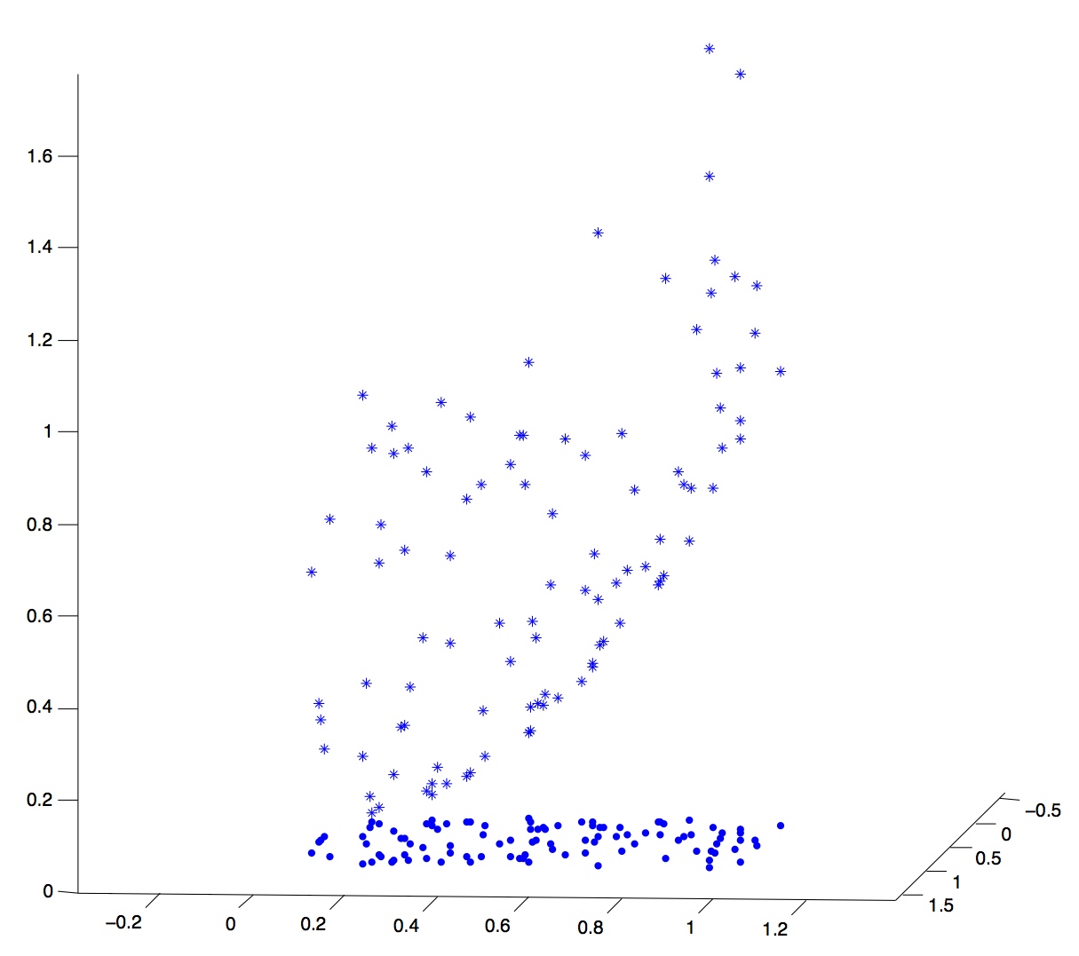
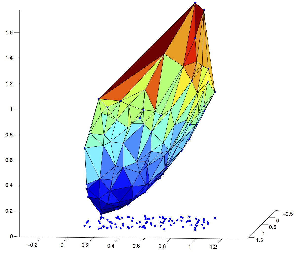
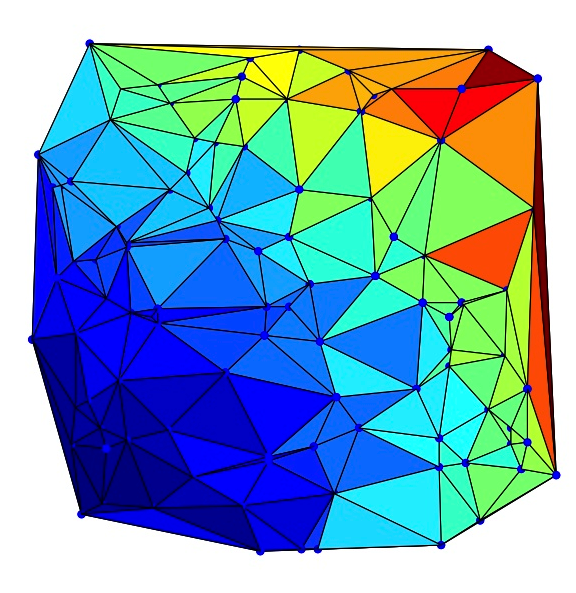
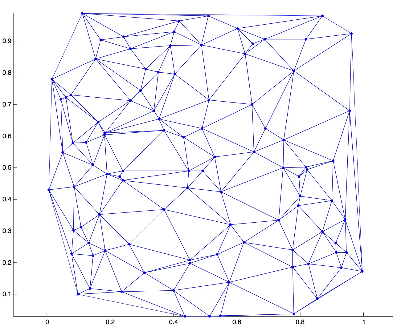
Thus to compute $\mathrm{PD}(V)$ and $\mathrm{DT}(V)$, we must compute a convex hull in $\mathbb{R}^{d+1}$. This is a well studied problem with numerous algorithms achieving optimal theoretical bounds in addition to others that work efficiently in practice. We highlight some of these algorithms here (let $C_{d+1}(N)$ denote the time needed to compute a convex hull of $N$ points in $\mathbb{R}^{d+1}$):

1. In [16, 38, 15] worst case algorithms for general dimension $d+1$ are given with complexity $C_{d+1}(N)=O(N\log N+N^{\lceil d/2\rceil})$. When $d=2$ this gives $O(N\log N)$ complexity. For higher dimensions, the worst case is rather pessimistic when one considers the average complexity over a family of convex hulls; see for example, [17].

2. In [37] an output sensitive algorithm for general dimension $d+1$ is given which achieves $C_{d+1}(N)=O(N^{2}+L\log L)$, where $L$ is the total number of faces of the convex hull.

3. For small dimensions greater than two, we have $C_{4}=O((N+L)\log^{2}L)$ [14] and $C_{5}=O((N+L)\log^{3}L)$ [2].

4. The QuickHull algorithm [10], while not having provable bounds on its complexity, is an output sensitive algorithm that empirically works very well. It is able to handle numerical errors caused by floating point arithmetic and is implemented for any dimension. In the online code associated to this paper, we utilize this algorithm.

3 Overview of the algorithm

The following is an overview of the algorithm for the Jet interpolation problem and the Function interpolation problem. The details of the algorithm are given in Sections 4, 5, and 6.

3.1 Jet interpolation problem

Input (jet): The set $E\subset\mathbb{R}^{d}$ having $N$ points and the $1$-field $P:E\rightarrow\mathcal{P}$, which consists of the function values $\{f_{a}\}_{a\in E}\subset\mathbb{R}$ and the gradients $\{D_{a}f\}_{a\in E}\subset\mathbb{R}^{d}$.

One time work, part I (jet): Compute $M=\mathrm{Lip}(\nabla F)$, for which there are two options:

1. $M=\Gamma^{1}(P;E)$ via direct calculation using (2.7), which requires $C\cdot d\cdot N^{2}$ work and $C\cdot d\cdot N$ storage.

2. Using the $\varepsilon$-WSPD of Section 2.3.1, compute an $M$ such that $cM\leq\Gamma^{1}(P;E)\leq M$, where $c<1$ is an absolute constant. The algorithm requires $(C\sqrt{d})^{d}\cdot N\log N$ work and $(C\sqrt{d})^{d}\cdot N$ storage.

Remark 3.1.

The choice depends on the relative sizes of $N$ and $d$, as well as the complexity of the remainder of the algorithm. For example, when $d=2$ and $N$ is large, in practice (see Section 7) this step is the bottleneck of the entire algorithm if one computes $M=\Gamma^{1}(P;E)$ exactly. In this case one might want to utilize the second computation, since it gains a significant speedup in $N$ while the exponential increase in $d$ is not much of a factor since $d=2$. On the other hand, the second algorithm is significantly more complicated to implement than the first, and scales poorly for high dimensional interpolation problems.

Output, part I (jet): $M=\mathrm{Lip}(\nabla F)$.

One time work, part II: Now we compute the underlying geometrical structures of Wells’ construction (Section 2.1) using the set $E$, the $1$-field $P:E\rightarrow\mathcal{P}$, and the value $M$ computed from the one time work, part I (jet). Recalling Wells’ set $\mathcal{K}$ from (2.3), define the following two related sets:

$$\widehat{\mathcal{K}}=\{\widehat{S}\mid S\in\mathcal{K}\},$$

$$\mathcal{K}_{\ast}=\{S_{\ast}\mid S\in\mathcal{K}\}.$$

A key observation is that $\mathcal{K}_{\ast}$ is the power diagram of the shifted points $\widetilde{E}=\{\tilde{a}\mid a\in E\}$, and that $\widehat{\mathcal{K}}$ is its dual triangulation. The power function is,

$$\mathrm{pow}(x,\tilde{a})=\frac{4}{M}d_{a}(x),$$

where $d_{a}$ is the distance function defined in (2.2), and the associated weight function is:

$$w(\tilde{a})=\frac{2}{M^{2}}|D_{a}f|^{2}-\frac{4}{M}f_{a}.$$

Sets $\{a\}_{\ast}\in\mathcal{K}_{\ast}$ correspond to nonempty power cells $\mathrm{cell}(\tilde{a})$, while sets $S_{\ast}$ for $\#(S)\geq 2$ are faces of the power diagram $\mathrm{PD}(\widetilde{E})$. Additionally, there is a clear bijective correspondence between $\mathcal{K}_{\ast}$ and $\widehat{\mathcal{K}}$, and furthermore $S_{\ast}\subseteq S_{\ast}^{\prime}$ if and only if $\widehat{S}^{\prime}\subseteq\widehat{S}$.

The main components of this part of the algorithm can be summarized as follows:

1. Compute the shifted points $\widetilde{E}=\{\tilde{a}\mid a\in E\}$. Requires $O(N)$ work and $O(N)$ storage.

2. Compute $\widehat{\mathcal{K}}=\mathrm{DT}(\widetilde{E})$ and $\mathcal{K}_{\ast}=\mathrm{PD}(\widetilde{E})$ by first lifting the shifted points into $\mathbb{R}^{d+1}$ via the map $\lambda$ in (2.8). Compute the convex hull of the lifted points, and project back down into $\mathbb{R}^{d}$. This gives $\mathrm{DT}(\widetilde{E})$. We store additionally for each $j$-dimensional face $\widehat{S}\in\widehat{\mathcal{K}}=\mathrm{DT}(\widetilde{E})$ ($0\leq j\leq d$), the $(j-1)$-dimensional faces contained in $\widehat{S}$ (i.e., its children) and the $(j+1)$-dimensional faces containing $\widehat{S}$ (i.e., its parents). Since $\mathcal{K}_{\ast}=\mathrm{PD}(\widetilde{E})$ is dual to $\mathrm{DT}(\widetilde{E})$, we can derive it via duality.

   The work of computing the convex hull is $O(N\log N+N^{\lceil d/2\rceil})$ and the storage for the convex hull (equivalently the triangulation/power diagram) is $O(N^{\lceil d/2\rceil})$ (see [8]). To calculate the children and parents for each face in $\mathrm{DT}(\widetilde{E})$ requires $O(N^{d+1})$ work and $O(N^{\lceil d/2\rceil+1})$ storage.

3. Determine the point $S_{C}$ for each $S\in\mathcal{K}$ and compute $d_{S}(S_{C})$. Requires $O(N^{d+1})$ and $O(N^{\lceil d/2\rceil})$ storage.

4. Compute the sets $\{T_{S}\}_{S\in\mathcal{K}}$ from $\widehat{\mathcal{K}}=\mathrm{DT}(\widetilde{E})$ and $\mathcal{K}_{\ast}=\mathrm{PD}(\widetilde{E})$. Store each set $T_{S}$ as a pair $(A_{S},b_{S})$, where $A_{S}$ is a matrix and $b_{S}$ is a vector, and $x\in T_{S}$ if and only if $A_{S}x\leq b_{S}$. Computing the full list of pairs $\{(A_{S},b_{S})\}_{S\in\mathcal{K}}$ requires $O(N^{d+2})$ work and $O(N^{\lceil d/2\rceil+1})$ storage.
   

Query work: Given a query point $x\in\mathbb{R}^{d}$, one must first determine which set $T_{S}$ it belongs to. There are two methods to accomplish this task:

1. A straightforward way is to check the inequalities $A_{S}x\leq b_{S}$ until one finds a pair $(A_{S},b_{S})$ that satisfies the condition for $x$. In the worst case, one will have to check all of the inequalities, which requires $O(N^{\lceil d/2\rceil+1})$ query work.

2. An alternate approach is to add an additional fifth step to the One time work, part II. In this step, one places a tree structure on the sets $\{T_{S}\}_{S\in\mathcal{K}}$ in which to each node we associate a hyperplane and the leaves correspond to the sets $\{T_{S}\}_{S\in\mathcal{K}}$. A query point $x$ is then passed down the tree according to whether it lies to the left or right of the hyperplane. If the tree is balanced, the query work is $O(\log N)$. An algorithm that can guarantee a balanced tree can be found in [23]; however, constructing the tree requires solving an optimization problem for which it is not easy to estimate the amount of work.

Once the query point is placed in the correct set $T_{S}$, the function $F_{S}$ is evaluated at $x$ and its gradient is computed. This requires an amount of work that is dependent only on the dimension $d$.

Output, part II: $F(x)$ and $\nabla F(x)$ for each query point $x\in\mathbb{R}^{d}$.

3.2 Function interpolation problem

In the case of the Function interpolation problem, we must amend the inputs and the first part of the one time work; the remainder of the algorithm is the same.

Input (function): The set $E\subset\mathbb{R}^{d}$ and the function $f:E\rightarrow\mathbb{R}$.

One time work, part I (function): Compute $M=\mathrm{Lip}(\nabla F)$ and $P_{a}=J_{a}F$, with $P_{a}(a)=f(a)$, for each $a\in E$. The scalar $M$ satisfies $cM-2\epsilon\leq\Gamma^{1}(f;E)\leq M$, with $c<1$ and $\epsilon>0$. The algorithm uses the $\varepsilon$-WSPD in conjunction with algorithms from convex optimization, and requires $O(N^{7/2}(\log N)^{1/2}\log(N/\epsilon))$ work.

Output, part I (function): $M=\mathrm{Lip}(\nabla F)$ as well as a $1$-field $P$ such that $\Gamma^{1}(P;E)=M$ and $P_{a}(a)=f(a)$ for all $a\in E$.

4 Computing $\Gamma^{1}$

We now describe algorithms for computing $\Gamma^{1}$ or the order of magnitude of $\Gamma^{1}$, for both the Jet interpolation problem and the Function interpolation problem.

4.1 Jet interpolation problem

For the Jet interpolation problem, as was discussed in Section 3, it is simple to compute $\Gamma^{1}(P;E)$ exactly in $C\cdot d\cdot N^{2}$ work. In this section we aim to improve the dependence on $N$ to be nearly linear, while sacrificing a small amount of accuracy and some efficiency in the dimension $d$. To that end, we prove the following theorem:

Theorem 4.1.

There is an algorithm, for which the inputs are the set $E\subset\mathbb{R}^{d}$ and the 1-field $P:E\rightarrow\mathcal{P}$, that computes a value $M$ satisfying:

$$M/C_{0}\leq\Gamma^{1}(P;E)\leq M,$$

where $C_{0}>1$ is an absolute constant. The algorithm requires $C(d)\cdot N\log N$ work and $C(d)\cdot N$ storage.

The plan for proving Theorem 4.1 is the following. First we view the $\Gamma^{1}(P;E)$ functional from the perspective of Whitney’s Extension Theorem (i.e., Theorem 1.1) for $C^{1,1}(\mathbb{R}^{d})$. Once we formalize this concept, we can use the $\varepsilon$-WSPD of Section 2.3.1, since it is constructed to handle interpolants in $C^{m}(\mathbb{R}^{d})$ satisfying Whitney conditions. The parameter $\varepsilon$ can be taken as any fixed number in $(0,1)$. The absolute constant $C_{0}$ of Theorem 4.1 decreases linearly with $\varepsilon$ as $C_{0}=2(1+\sqrt{2})(3+23\varepsilon)$. However the dimensional constant $C(d)$ increases exponentially with $d$, and in particular $C(d)=(C\cdot\sqrt{d}/\varepsilon)^{d}$ for any $\varepsilon\leq 1/2$ (see Remark 2.5).

Concerning the first part of our approach, recall that if we take the infimum over all $M$ satisfying the Whitney conditions $(W_{0})$ and $(W_{1})$, then we obtain a value that is within a constant $C^{\prime}(d)$ of $\|P\|_{C^{1,1}(E)}$. The main contribution of [33] is to refine $(W_{0})$ and $(W_{1})$ so that $C^{\prime}(d)=1$; this is $\Gamma^{1}(P;E)$. Indeed, referring to the alternate form of $\Gamma^{1}(P;E)$ given in (2.7), the functional $A$ corresponds to $(W_{0})$, the functional $B$ corresponds to $(W_{1})$, and $\Gamma^{1}(P;E)$ pieces them together. Note there are some small, but significant differences. In particular, the functional $A$ is essentially a symmetric version of $(W_{0})$; using one is equivalent to using the other, up to a factor of two. The functional $B$ though, merges all of the partial derivative information into one condition, unlike $(W_{1})$. Thus they are equivalent only up to a factor of $d$, the dimension of the Euclidean space we are working in. For the algorithm in this section, we will use the functional $B$ since it is both simpler and more useful than $(W_{1})$, but use $(W_{0})$ instead of $A$. Additionally, we will treat them separately instead of together like in $\Gamma^{1}(P;E)$; Lemma 4.2 contains the details.

For the 1-field $P:E\rightarrow\mathcal{P}$, define the functional $\widetilde{A}$, which is essentially the same as $(W_{0})$:

$$\widetilde{A}(P;a,b)=\frac{|P_{a}(a)-P_{b}(a)|}{|a-b|^{2}},\quad a,b\in E.$$

Additionally, set

$$\widetilde{\Gamma}^{1}(P;E)=\max_{\begin{subarray}{c}a,b\in E\\ a\neq b\end{subarray}}\Big{\{}\max\{\widetilde{A}(P;a,b),B(P;a,b)\}\Big{\}}.$$

The functional $\widetilde{\Gamma}^{1}(P;E)$ is more easily approximated via the $\varepsilon$-WSPD than $\Gamma^{1}(P;E)$. Furthermore, as the following lemma shows, they have the same order of magnitude.

Lemma 4.2.

For any finite set $E\subset\mathbb{R}^{d}$ and any 1-field $P:E\rightarrow\mathcal{P}$,

$$\widetilde{\Gamma}^{1}(P;E)\leq\Gamma^{1}(P;E)\leq 2(1+\sqrt{2})\widetilde{\Gamma}^{1}(P;E).$$

Proof.

To bridge the gap between $\Gamma^{1}(P;E)$ and $\widetilde{\Gamma}^{1}(P;E)$, we first consider

$$\overline{\Gamma}^{1}(P;E)=\max_{\begin{subarray}{c}a,b\in E\\ a\neq b\end{subarray}}\Big{\{}\max\{A(P;a,b),B(P;a,b)\}\Big{\}}.$$

Clearly $\overline{\Gamma}^{1}(P;E)\leq\Gamma^{1}(P;E)$. Furthermore,

$$\Gamma^{1}(P;E) =\max_{\begin{subarray}{c}a,b\in E\\ a\neq b\end{subarray}}\sqrt{A(P;a,b)^{2}+B(P;a,b)^{2}}+A(P;a,b)$$

$$\leq\sqrt{\overline{\Gamma}^{1}(P;E)^{2}+\overline{\Gamma}^{1}(P;E)^{2}}+\overline{\Gamma}^{1}(P;E)$$

$$\leq(1+\sqrt{2})\overline{\Gamma}^{1}(P;E).$$

Thus $\Gamma^{1}(P;E)$ and $\overline{\Gamma}^{1}(P;E)$ have the same order of magnitude, and in particular,

(4.1) $$\overline{\Gamma}^{1}(P;E)\leq\Gamma^{1}(P;E)\leq(1+\sqrt{2})\overline{\Gamma}^{1}(P;E).$$

Now let us consider $\overline{\Gamma}^{1}(P;E)$ and $\widetilde{\Gamma}^{1}(P;E)$ (which means considering $A(P;a,b)$ and $\widetilde{A}(P;a,b)$). First,

$$|P_{a}(a)-P_{b}(a)+P_{a}(b)-P_{b}(b)| \leq|P_{a}(a)-P_{b}(a)|+|P_{a}(b)-P_{b}(b)|$$

$$\leq 2\widetilde{\Gamma}^{1}(P;E)|a-b|^{2},$$

and so, $\overline{\Gamma}^{1}(P;E)\leq 2\widetilde{\Gamma}^{1}(P;E)$. For a reverse inequality, we note,

$$|P_{a}(a)-P_{b}(a)+P_{a}(b)-P_{b}(b)|=|2(P_{a}(a)-P_{b}(a))+(\nabla P_{b}-\nabla P_{a})\cdot(a-b)|.$$

Thus,

$$2|P_{a}(a)-P_{b}(a)| \leq\overline{\Gamma}^{1}(P;E)|a-b|^{2}+|(\nabla P_{b}-\nabla P_{a})\cdot(a-b)|$$

$$\leq 2\overline{\Gamma}^{1}(P;E)|a-b|^{2},$$

which yields $\widetilde{\Gamma}^{1}(P;E)\leq\overline{\Gamma}^{1}(P;E)$. Combining the two inequalities,

(4.2) $$\widetilde{\Gamma}^{1}(P;E)\leq\overline{\Gamma}^{1}(P;E)\leq 2\widetilde{\Gamma}^{1}(P;E).$$

Putting (4.1) and (4.2) together completes the proof. ∎

We will also need the following simple lemmas.

Lemma 4.3.

Let $(\mathcal{T},\mathcal{W})$ be a $\varepsilon$-WSPD, $(\Lambda_{1},\Lambda_{2})\in\mathcal{W}$, $x,x^{\prime},x^{\prime\prime}\in\cup\Lambda_{1}$, and $y,y^{\prime}\in\cup\Lambda_{2}$. Then,

$$|x^{\prime}-x^{\prime\prime}|\leq\varepsilon|x-y|$$

$$|x^{\prime}-y^{\prime}|\leq(1+2\varepsilon)|x-y|.$$

Proof.

Use the definition of $\varepsilon$-separated. ∎

Lemma 4.4.

Suppose $p\in\mathcal{P}$, $x\in\mathbb{R}^{d}$, $\delta>0$, and $M>0$ satisfy

$$|p(x)|\leq M\delta^{2}$$

$$|\nabla p(x)|\leq M\delta.$$

Then, for any $y\in\mathbb{R}^{d}$,

$$|p(y)|\leq M(\delta+|x-y|)^{2}.$$

Proof.

Using Taylor’s Theorem,

$$|p(y)| =|p(x)+\nabla p(x)\cdot(y-x)|$$

$$\leq|p(x)|+|\nabla p(x)||x-y|$$

$$\leq M\delta^{2}+M\delta|x-y|$$

$$\leq M(\delta+|x-y|)^{2}.$$

∎

Proof of Theorem 4.1.

Set:

$$\widetilde{A}(P;E) =\max_{\begin{subarray}{c}a,b\in E\\ a\neq b\end{subarray}}\widetilde{A}(P;a,b),$$

$$B(P;E) =\max_{\begin{subarray}{c}a,b\in E\\ a\neq b\end{subarray}}B(P;a,b),$$

and note that $\widetilde{\Gamma}^{1}(P;E)=\max\{\widetilde{A}(P;E),\,B(P;E)\}$.

Our algorithm works as follows. For now, let $0<\varepsilon<1$ be arbitrary and invoke the algorithm from Theorem 2.4. This gives us an $\varepsilon$-WSPD $(\mathcal{T},\mathcal{W})$ in $C(\varepsilon,d)N\log N$ work and using $C(\varepsilon,d)N$ storage. For each $(\Lambda_{1},\Lambda_{2})\in\mathcal{W}$, pick a representative pair $(a_{\Lambda_{1}},a_{\Lambda_{2}})\in\cup\Lambda_{1}\times\cup\Lambda_{2}$. Additionally, for each $S\in\mathcal{T}$, pick a representative $a_{S}\in S$.

We now compute the following:

$$\widetilde{A}_{1}(P;\mathcal{T},\mathcal{W}) =\max_{(\Lambda_{1},\Lambda_{2})\in\mathcal{W}}\widetilde{A}(P;a_{\Lambda_{1}},a_{\Lambda_{2}}),$$

(4.3) $$\widetilde{A}_{2}(P;\mathcal{T},\mathcal{W}) =\max_{(\Lambda_{1},\Lambda_{2})\in\mathcal{W}}\,\max_{i=1,2}\,\max_{S\in\Lambda_{i}}\widetilde{A}(P;a_{\Lambda_{i}},a_{S}),$$

$$\widetilde{A}_{3}(P;\mathcal{T},\mathcal{W}) =\max_{S\in\mathcal{T}}\max_{a\in S}\widetilde{A}(P;a,a_{S}),$$

and

$$B_{1}(P;\mathcal{T},\mathcal{W}) =\max_{(\Lambda_{1},\Lambda_{2})\in\mathcal{W}}B(P;a_{\Lambda_{1}},a_{\Lambda_{2}}),$$

$$B_{2}(P;\mathcal{T},\mathcal{W}) =\max_{(\Lambda_{1},\Lambda_{2})\in\mathcal{W}}\,\max_{i=1,2}\,\max_{S\in\Lambda_{i}}B(P;a_{\Lambda_{i}},a_{S}),$$

$$B_{3}(P;\mathcal{T},\mathcal{W}) =\max_{S\in\mathcal{T}}\max_{a\in S}B(P;a,a_{S}).$$

Additionally, compute:

$$\widetilde{A}(P;\mathcal{T},\mathcal{W}) =\max_{i=1,2,3}\widetilde{A}_{i}(P;\mathcal{T},\mathcal{W}),$$

$$B(P;\mathcal{T},\mathcal{W}) =\max_{i=1,2,3}B_{i}(P;\mathcal{T},\mathcal{W}),$$

as well as

(4.4) $$\widetilde{\Gamma}^{1}(P;\mathcal{T},\mathcal{W})=\max\{\widetilde{A}(P;\mathcal{T},\mathcal{W}),\,B(P;\mathcal{T},\mathcal{W})\}.$$

Using properties 6 and 7 from Section 2.3.1, we see that computing $\widetilde{\Gamma}^{1}(P;\mathcal{T},\mathcal{W})$ requires $C(\varepsilon,d)N\log N$ work and $C(\varepsilon,d)N$ storage.

Now we show that $\widetilde{\Gamma}^{1}(P;\mathcal{T},\mathcal{W})$ has the same order of magnitude as $\widetilde{\Gamma}^{1}(P;E)$. Clearly, $\widetilde{\Gamma}^{1}(P;\mathcal{T},\mathcal{W})\leq\widetilde{\Gamma}^{1}(P;E)$. For the other inequality, we break $\widetilde{\Gamma}^{1}(P;E)$ into its two parts. Since $\widetilde{\Gamma}^{1}(P;E)=\max\{\widetilde{A}(P;E),\,B(P;E)\}$, it suffices to show that $\widetilde{A}(P;E)$ and $B(P;E)$ are each bounded from above by $C(\varepsilon)\cdot\widetilde{\Gamma}^{1}(P;\mathcal{T},\mathcal{W})$.

Set:

$$\widetilde{\Gamma}_{i}^{1}(P;\mathcal{T},\mathcal{W})=\max\{\widetilde{A}_{i}(P;\mathcal{T},\mathcal{W}),B_{i}(P;\mathcal{T},\mathcal{W})\},\quad i=1,2,3,$$

and note $\widetilde{\Gamma}_{i}^{1}(P;\mathcal{T},\mathcal{W})\leq\widetilde{\Gamma}^{1}(P;\mathcal{T},\mathcal{W})$ for each $i=1,2,3$.

Let $a,b\in E$, $a\neq b$. By properties 1 and 2 of Section 2.3.1, there is a unique pair $(\Lambda_{1},\Lambda_{2})\in\mathcal{W}$ such that $(a,b)\in\cup\Lambda_{1}\times\cup\Lambda_{2}$. Additionally, by the definition of $(\mathcal{T},\mathcal{W})$, there exists a set $S\in\Lambda_{1}$ such that $a\in S$ and a set $T\in\Lambda_{2}$ such that $b\in T$.

We first bound $\widetilde{A}(P;E)$. Using the triangle inequality, the definition of $\widetilde{A}_{3}(P;\mathcal{T},\mathcal{W})$, and Lemma 4.3,

$$|P_{a}(a)-P_{b}(a)| \leq|P_{a}(a)-P_{a_{S}}(a)|+|P_{a_{S}}(a)-P_{b}(a)|$$

$$\leq\widetilde{A}_{3}(P;\mathcal{T},\mathcal{W})\cdot|a-a_{S}|^{2}+|P_{a_{S}}(a)-P_{b}(a)|$$

(4.5) $$\leq\varepsilon\cdot\widetilde{\Gamma}^{1}(P;\mathcal{T},\mathcal{W})\cdot|a-b|^{2}+|P_{a_{S}}(a)-P_{b}(a)|.$$

We continue with the second term of the right hand side of (4.5). Using the triangle inequality, Lemma 4.4 applied to $P_{a_{S}}-P_{a_{\Lambda_{1}}}$ with $x=a_{\Lambda_{1}}$, $y=a$ and $M=\widetilde{\Gamma}_{2}^{1}(P;\mathcal{T},\mathcal{W})$, as well as Lemma 4.3, we obtain:

$$|P_{a_{S}}(a)-P_{b}(a)| \leq|P_{a_{S}}(a)-P_{a_{\Lambda_{1}}}(a)|+|P_{a_{\Lambda_{1}}}(a)-P_{b}(a)|$$

$$\leq\widetilde{\Gamma}^{1}_{2}(P;\mathcal{T},\mathcal{W})\cdot(|a_{S}-a_{\Lambda_{1}}|+|a-a_{\Lambda_{1}}|)^{2}+|P_{a_{\Lambda_{1}}}(a)-P_{b}(a)|$$

(4.6) $$\leq 4\varepsilon^{2}\cdot\widetilde{\Gamma}^{1}(P;\mathcal{T},\mathcal{W})\cdot|a-b|^{2}+|P_{a_{\Lambda_{1}}}(a)-P_{b}(a)|.$$

To bound the second term of the right hand side of (4.6), we use the triangle inequality, Lemma 4.4 applied to $P_{b}-P_{a_{T}}$ with $x=b$, $y=a$ and $M=\widetilde{\Gamma}_{3}^{1}(P;\mathcal{T},\mathcal{W})$, and Lemma 4.3:

$$|P_{a_{\Lambda_{1}}}(a)-P_{b}(a)| \leq|P_{b}(a)-P_{a_{T}}(a)|+|P_{a_{T}}(a)-P_{a_{\Lambda_{1}}}(a)|$$

$$\leq\widetilde{\Gamma}^{1}_{3}(P;\mathcal{T},\mathcal{W})\cdot(|b-a_{T}|+|a-b|)^{2}+|P_{a_{T}}(a)-P_{a_{\Lambda_{1}}}(a)|$$

(4.7) $$\leq(1+\varepsilon)^{2}\cdot\widetilde{\Gamma}^{1}(P;\mathcal{T},\mathcal{W})\cdot|a-b|^{2}+|P_{a_{T}}(a)-P_{a_{\Lambda_{1}}}(a)|.$$

Finally, for the second term of the right hand side of (4.7), we use the triangle inequality, Lemma 4.4 applied to $P_{a_{T}}-P_{a_{\Lambda_{2}}}$ with $x=a_{\Lambda_{2}}$, $y=a$ and $M=\widetilde{\Gamma}_{2}^{1}(P;\mathcal{T},\mathcal{W})$, Lemma 4.4 applied to $P_{a_{\Lambda_{2}}}-P_{a_{\Lambda_{1}}}$ with $x=a_{\Lambda_{1}}$, $y=a$ and $M=\widetilde{\Gamma}_{1}^{1}(P;\mathcal{T},\mathcal{W})$, as well as Lemma 4.3:

$$|P_{a_{T}}(a) -P_{a_{\Lambda_{1}}(a)}(a)|$$

$$\leq|P_{a_{T}}(a)-P_{a_{\Lambda_{2}}}(a)|+|P_{a_{\Lambda_{2}}}(a)-P_{a_{\Lambda_{1}}}(a)|$$

$$\leq\widetilde{\Gamma}_{2}^{1}(P;\mathcal{T},\mathcal{W})\cdot(|a_{T}-a_{\Lambda_{2}}|+|a-a_{\Lambda_{2}}|)^{2}+|P_{a_{\Lambda_{2}}}(a)-P_{a_{\Lambda_{1}}}(a)|$$

$$\leq(1+3\varepsilon)^{2}\cdot\widetilde{\Gamma}^{1}(P;\mathcal{T},\mathcal{W})\cdot|a-b|^{2}+\widetilde{\Gamma}^{1}_{1}(P;\mathcal{T},\mathcal{W})\cdot(|a_{\Lambda_{2}}-a_{\Lambda_{1}}|+|a-a_{\Lambda_{1}}|)^{2}$$

(4.8) $$\leq 2(1+3\varepsilon)^{2}\cdot\widetilde{\Gamma}^{1}(P;\mathcal{T},\mathcal{W})\cdot|a-b|^{2}.$$

Putting (4.5), (4.6), (4.7), (4.8) together, we get:

(4.9) $$|P_{a}(a)-P_{b}(a)|\leq(3+23\varepsilon)\cdot\widetilde{\Gamma}^{1}(P;\mathcal{T},\mathcal{W})\cdot|a-b|^{2}.$$

The proof for $B(P;E)$ proceeds along similar lines. Using the same sequence of triangle inequalities, in addition to several applications of Lemma 4.3, yields:

$$|D_{a}f-D_{b}f|\leq{} |D_{a}f-D_{a_{S}}f|+|D_{a_{S}}f-D_{a_{\Lambda_{1}}}f|+|D_{a_{\Lambda_{1}}}f-D_{a_{\Lambda_{2}}}f|$$

$$+|D_{a_{\Lambda_{2}}}f-D_{a_{T}}f|+|D_{a_{T}}f-D_{b}f|$$

$$\leq{} B_{3}(P;\mathcal{T},\mathcal{W})\cdot|a-a_{S}|+B_{2}(P;\mathcal{T},\mathcal{W})\cdot|a_{S}-a_{\Lambda_{1}}|$$

$$+B_{1}(P;\mathcal{T},\mathcal{W})\cdot|a_{\Lambda_{1}}-a_{\Lambda_{2}}|+B_{2}(P;\mathcal{T},\mathcal{W})\cdot|a_{\Lambda_{2}}-a_{T}|$$

$$+B_{1}(P;\mathcal{T},\mathcal{W})\cdot|a_{T}-b|$$

(4.10) $$\leq{} (1+6\varepsilon)\cdot\widetilde{\Gamma}^{1}(P;\mathcal{T},\mathcal{W})\cdot|a-b|.$$

Combining (4.9) and (4.10) gives:

$$\widetilde{\Gamma}^{1}(P;\mathcal{T},\mathcal{W})\leq\widetilde{\Gamma}^{1}(P;E)\leq(3+23\varepsilon)\cdot\widetilde{\Gamma}^{1}(P;\mathcal{T},\mathcal{W}).$$

Now apply Lemma 4.2 to obtain:

$$\widetilde{\Gamma}^{1}(P;\mathcal{T},\mathcal{W})\leq\Gamma^{1}(P;E)\leq 2(1+\sqrt{2})(3+23\varepsilon)\cdot\widetilde{\Gamma}^{1}(P;\mathcal{T},\mathcal{W}).$$

The proof is completed by selecting any $\varepsilon\in(0,1)$. ∎

4.2 Function interpolation problem

4.2.1 Convex optimization

For the Function interpolation problem, we have only the function values $f:E\rightarrow\mathbb{R}$ and we must compute:

$$\Gamma^{1}(f;E)=\inf\{\Gamma^{1}(P;E)\mid P_{a}(a)=f(a)\text{ for all }a\in E\}.$$

Recall that $P_{a}(x)=f_{a}+D_{a}f\cdot(x-a)$. Since we must have $P_{a}(a)=f_{a}=f(a)$, the values $\{f_{a}\}_{a\in E}$ are fixed. Additionally, the set $E$ is fixed. Therefore, we must solve for the gradients $\{D_{a}f\}_{a\in E}$ that minimize $\Gamma^{1}(P;E)$. Thus in this section we view $\Gamma^{1}(P;E)$ as a function of the gradients. In order to clarify this point, let $E=\{a_{k}\}_{k=1}^{N}$ be an indexation of $E$ and define a new variable $Y=(y_{1},\ldots,y_{N})\in\mathbb{R}^{dN}$ with $y_{k}\in\mathbb{R}^{d}$ for each $k=1,\ldots,N$. Let $g:\mathbb{R}^{dN}\rightarrow\mathbb{R}$ be defined as:

$$g(Y)=\Gamma^{1}(P;E),\quad P_{a_{k}}(x)=f(a_{k})+y_{k}\cdot(x-a_{k}).$$

The function $g:\mathbb{R}^{dN}\rightarrow\mathbb{R}$ is a convex function and since $\Gamma^{1}(P;E)>0$ it is piecewise twice differentiable. Therefore we can use algorithms from convex optimization to solve for $\Gamma^{1}(f;E)$. Indeed, consider the following unconstrained convex optimization problem:

(4.11) $$\text{minimize}\quad g(Y).$$

The value of (4.11) is $\Gamma^{1}(f;E)$. Additionally, if $Y^{\star}=(y_{1}^{\star},\ldots,y_{N}^{\star})$ is the minimizer, then the $1$-field $P^{\star}$ defined by

$$P_{a_{k}}^{\star}(x)=f(a_{k})+y_{k}^{\star}\cdot(x-a_{k}),$$

achieves the value $\Gamma^{1}(f;E)$. One can solve (4.11) using Newton’s method. A rigorous estimate for the number of iterations (in particular the number of Newton steps) is difficult to compute due to the square root in the $\Gamma^{1}$ functional, but we can examine a related convex optimization problem to get a related estimate.

Recall the functional $\widetilde{\Gamma}^{1}(P;E)$, which has the same order of magnitude as $\Gamma^{1}$, and was defined as:

$$\widetilde{\Gamma}^{1}(P;E)=\max_{\begin{subarray}{c}a,b,\in E\\ a\neq b\end{subarray}}\left\{\widetilde{A}(P;a,b),B(P;a,b)\right\}.$$

Define $\widetilde{\Gamma}^{1}(f;E)$ analogously to $\Gamma^{1}(f;E)$,

$$\widetilde{\Gamma}^{1}(f;E)=\inf\{\widetilde{\Gamma}^{1}(P;E)\mid P_{a}(a)=f(a)\text{ for all }a\in E\},$$

and similarly define $\tilde{g}:\mathbb{R}^{dN}\rightarrow\mathbb{R}$ analogously to $g$. Then the following unconstrained convex optimization problem solves for $\widetilde{\Gamma}^{1}(f;E)$:

(4.12) $$\text{minimize}\quad\tilde{g}(Y).$$

We can rewrite (4.12) in a form that is more easily accessible and that utilizes only continuous, twice differentiable functions (as opposed to $\tilde{g}$ which is piecewise such). Related to the functional $\widetilde{A}$, define two families of functions $\alpha_{j,k}^{+}:\mathbb{R}^{dN+1}\rightarrow\mathbb{R}$ and $\alpha_{j,k}^{-}:\mathbb{R}^{dN+1}\rightarrow\mathbb{R}$,

$$\alpha_{j,k}^{+}(Y,M) =y_{k}\cdot(a_{k}-a_{j})-M|a_{j}-a_{k}|^{2}+f(a_{j})-f(a_{k}),\quad j,k=1,\ldots,N,$$

$$\alpha_{j,k}^{-}(Y,M) =y_{k}\cdot(a_{j}-a_{k})-M|a_{j}-a_{k}|^{2}+f(a_{k})-f(a_{j}),\quad j,k=1,\ldots,N,$$

where $M\in\mathbb{R}$. Additionally, for the functional $B$ define $\beta_{j,k}:\mathbb{R}^{dN+1}\rightarrow\mathbb{R}$,

$$\beta_{j,k}(Y,M)=|y_{j}|^{2}+|y_{k}|^{2}-2y_{j}\cdot y_{k}-M^{2}|a_{j}-a_{k}|^{2},\quad j,k=1,\ldots,N.$$

Then the following optimization problem is equivalent to (4.12):

(4.13) minimize $$\quad M,$$

subject to $$\quad\alpha_{j,k}^{+}(Y,M)\leq 0,\quad\forall\,j,k=1,\ldots,N,$$

$$\quad\alpha_{j,k}^{-}(Y,M)\leq 0,\quad\forall\,j,k=1,\ldots,N,$$

$$\quad\beta_{j,k}(Y,M)\leq 0,\quad\forall\,j,k=1,\ldots,N.$$

Indeed, if $(Y^{\star},M^{\star})$ is the minimizer, then $\widetilde{\Gamma}^{1}(f;E)=M^{\star}$ and $Y^{\star}$ defines the gradients of the $1$-field $P^{\star}$ such that $\widetilde{\Gamma}^{1}(P^{\star};E)=M^{\star}$.

Constrained convex optimization problems can be solved using interior point methods. In Appendix A we describe a particular form of the barrier method that iteratively solves a sequence of unconstrained optimization problems with Newton’s method. Each iteration is referred to as a Newton step.

The $\alpha$ functions are linear and the $\beta$ functions are quadratic; therefore, (4.13) is a quadratically constrained quadratic program (QCQP). Thus Theorem A.1 from Appendix A applies and we see that the number of Newton steps required for the barrier method to solve (4.13) to within (additive) accuracy $\epsilon$ is $O(N\log(N/\epsilon))$.

The cost of each Newton step can be derived from equations (A.5) and (A.7) (also in Appendix A). Without considering any structure in the problem, the amount of work is $O(N^{4})$ due to the cost of forming the relevant Hessian matrix $H$. However, each $\alpha$ and $\beta$ function depends only on $2d+1$ variables; therefore the cost of forming $H$ is in fact $O(N^{2})$. In this case the Cholesky factorization for computing $H^{-1}$ will dominate with $O(N^{3})$ work per Newton step. Thus the total work is $O(N^{4}\log(N/\epsilon))$. We collect this result in the following proposition.

Proposition 4.5.

There is an algorithm, for which the inputs are the set $E\subset\mathbb{R}^{d}$, the function $f:E\rightarrow\mathbb{R}$ and a parameter $\epsilon>0$, that computes a value $\widetilde{M}$ satisfying:

$$\widetilde{M}-\epsilon\leq\widetilde{\Gamma}^{1}(f;E)\leq\widetilde{M}+\epsilon,$$

as well as a $1$-field $P$ such that $\Gamma^{1}(P;E)=\widetilde{M}$ and $P_{a}(a)=f(a)$ for all $a\in E$. The algorithm requires $O(N^{4}\log(N/\epsilon))$ work.

As a corollary we have:

Corollary 4.6.

There is an algorithm, for which the inputs are the set $E\subset\mathbb{R}^{d}$, the function $f:E\rightarrow\mathbb{R}$ and a parameter $\epsilon>0$, that computes a value $M$ satisfying:

$$M/C-2\epsilon\leq\Gamma^{1}(f;E)\leq M,$$

where $C=2(1+\sqrt{2})$. The algorithm also outputs a $1$-field $P$ such that $\Gamma^{1}(P;E)=M$ and $P_{a}(a)=f(a)$ for all $a\in E$. The work required is $O(N^{4}\log(N/\epsilon))$.

4.2.2 Convex optimization + $\varepsilon$-WSPD

As in the Jet interpolation problem, one can reduce the amount of work by utilizing the $\varepsilon$-WSPD and computing a value $\widetilde{M}$ that is within a multiplicative constant of $\widetilde{\Gamma}^{1}(f;E)$.

Recall from the proof of Theorem 4.1 the constant $\widetilde{\Gamma}^{1}(P;\mathcal{T},\mathcal{W})$ defined in (4.4), which has the same order of magnitude as $\Gamma^{1}(P;E)$. It is computed over pairs of points $(E\times E)_{\mathcal{T},\mathcal{W}}\subset E\times E$ derived from the $\varepsilon$-WSPD $(\mathcal{T},\mathcal{W})$ of Section 2.3.1; recall these pairs are (see (4.3)):

$$(E\times E)_{\mathcal{T},\mathcal{W}}={} \{(a_{\Lambda_{1}},a_{\Lambda_{2}})\mid(\Lambda_{1},\Lambda_{2})\in\mathcal{W}\}\,\cup$$

$$\{(a_{\Lambda_{i}},a_{S})\mid(\Lambda_{1},\Lambda_{2})\in\mathcal{W},\,i=1,2,\,S\in\Lambda_{i}\}\,\cup$$

$$\{(a,a_{S})\mid S\in\mathcal{T},\,a\in S\}.$$

Let $(\mathbb{Z}_{N}\times\mathbb{Z}_{N})_{\mathcal{T},\mathcal{W}}\subset\mathbb{Z}_{N}\times\mathbb{Z}_{N}$ denote the indices of these pairs. Consider the following optimization problem:

(4.14) minimize $$\quad M,$$

subject to $$\quad\alpha_{j,k}^{+}(Y,M)\leq 0,\quad\forall\,(j,k)\in(\mathbb{Z}_{N}\times\mathbb{Z}_{N})_{\mathcal{T},\mathcal{W}},$$

$$\quad\alpha_{j,k}^{-}(Y,M)\leq 0,\quad\forall\,(j,k)\in(\mathbb{Z}_{N}\times\mathbb{Z}_{N})_{\mathcal{T},\mathcal{W}},$$

$$\quad\beta_{j,k}(Y,M)\leq 0,\quad\forall\,(j,k)\in(\mathbb{Z}_{N}\times\mathbb{Z}_{N})_{\mathcal{T},\mathcal{W}}.$$

The minimizer of (4.14) is $\widetilde{\Gamma}^{1}(f;\mathcal{T},\mathcal{W})$, which is defined as:

$$\widetilde{\Gamma}^{1}(f;\mathcal{T},\mathcal{W})=\inf\{\widetilde{\Gamma}^{1}(P;\mathcal{T},\mathcal{W})\mid P_{a}(a)=f(a)\text{ for all }a\in E\}.$$

By Theorem 4.1 it has the same order of magnitude as $\Gamma^{1}(f;E)$. Additionally, by construction of the $\varepsilon$-WSPD $(\mathcal{T},\mathcal{W})$, $(\mathbb{Z}_{N}\times\mathbb{Z}_{N})_{\mathcal{T},\mathcal{W}}$ has only $O(N\log N)$ pairs of points. Thus Theorem A.1 implies the number of Newton steps required for the barrier method is $O((N\log N)^{1/2}\log(N/\epsilon))$.

The cost per Newton step is harder to bound rigorously. The amount of work to form the relevant Hessian matrix $H$ is $O(N\log N)$. Furthermore, the Hessian matrix is sparse, with only $O(N\log N)$ nonzero entries. Thus, for the Cholesky factorization, we can use a sparse factorization algorithm. However, an exact bound on the work required depends on the sparsity pattern. In fact we know the pattern, since it can be derived from the $\varepsilon$-WSPD, however, to the best of our knowledge there is no theorem relating well separated pair decompositions and sparse Cholesky factorization algorithms. For sparse matrices corresponding to planar graphs, the storage is $O(N\log N)$ and the work is $O(N^{3/2})$ for the Cholesky factorization [34]; one might hope a similar theorem could be proved for the Hessian matrix derived from the $\varepsilon$-WSPD. As it stands currently, we are guaranteed no more than $O(N^{7/2}(\log N)^{1/2}\log(N/\epsilon))$ work:

Proposition 4.7.

There is an algorithm, for which the inputs are the set $E\subset\mathbb{R}^{d}$, the function $f:E\rightarrow\mathbb{R}$ and a parameter $\epsilon>0$, that computes a value $M$ satisfying:

$$M/C_{0}-2\epsilon\leq\Gamma^{1}(f;E)\leq M,$$

where $C_{0}$ is the same absolute constant of Theorem 4.1. The algorithm also outputs $1$-field $P$ such that $\Gamma^{1}(P;E)=M$ and $P_{a}(a)=f(a)$ for all $a\in E$. The work required is $O(N^{7/2}(\log N)^{1/2}\log(N/\epsilon))$.

5 One time work, part II

At this point in the algorithm we have computed a value $M=\mathrm{Lip}(\nabla F)$ such that $M=\Gamma^{1}$ (either the jet or function version) or $M$ has the same order of magnitude as $\Gamma^{1}$. Additionally we have a 1-field $P:E\rightarrow\mathcal{P}$ regardless of whether we started with the Jet interpolation problem or the Function interpolation problem.

Let

$$E=\{a_{k}\mid k=1,\ldots,N\},$$

be an indexation of the set $E$. The first step is to compute the shifted points:

$$\widetilde{E}=\{\tilde{a}_{k}=a_{k}-D_{a_{k}}f/M\mid k=1,\ldots,N\}.$$

Clearly this requires $O(N)$ work and $O(N)$ storage.

5.1 Computing $\mathcal{K}_{\ast}$ and $\widehat{\mathcal{K}}$

With $\widetilde{E}$ in hand, we compute the power diagram $\mathcal{K}_{\ast}=\mathrm{PD}(\widetilde{E})$ and the dual triangulation $\widehat{\mathcal{K}}=\mathrm{DT}(\widetilde{E})$. We employ the lifting procedure via the map $\lambda:\widetilde{E}\rightarrow\mathbb{R}^{d+1}$ described in Section 2.3.2. Once the points have been lifted, we compute the convex hull of $\lambda(\widetilde{E})$. To determine the lower hull, we compute a normal vector for each $d$-dimensional facet of the convex hull, and orient them so that they are pointing inward. The inward pointing normals determine the facets of the lower hull (namely, if the $x_{d+1}$ coordinate of the normal is positive, then the facet is on the lower hull). We then orthogonally project the facets of the lower hull onto $\mathbb{R}^{d}$, under the map $(x_{1},\ldots,x_{d},x_{d+1})\mapsto(x_{d},\ldots,x_{d})$. This gives us the triangulation $\widehat{\mathcal{K}}=\mathrm{DT}(\widetilde{E})$. It is initially stored in a data a structure which lists the $d$-dimensional faces, which are simplices. Each simplex is uniquely determined by storing the $d+1$ indices $\{k_{i}\}_{i=1}^{d+1}$ which correspond to the vertices $\{\tilde{a}_{k_{i}}\}_{i=1}^{d+1}$ of the simplex. The work is $O(N\log N+N^{\lceil d/2\rceil})$ and the storage is $O(N^{\lceil d/2\rceil})$.

We make a pass through the simplices of the triangulation and store, for each simplex, the $(d-1)$-dimensional facets contained in that simplex, which we refer to as its children. Proceeding in a top-down fashion, we store for each $j$-dimensional face $\widehat{S}\in\widehat{\mathcal{K}}=\mathrm{DT}(\widetilde{E})$ ($0<j<d$), both its children, which are the $(j-1)$-dimensional faces of $\mathrm{DT}(\widetilde{E})$ contained in $\widehat{S}$, and its parents, which are the $(j+1)$-dimensional faces of $\mathrm{DT}(\widetilde{E})$ that contain $\widehat{S}$. For the vertices $\widetilde{E}$, we store only the parents of each vertex, since they have no children. Each $j$-dimensional face ($0<j\leq d$) has exactly $j+1$ children. Additionally, the number of parents per face is no more than $N$. Since there are $O(N^{\lceil d/2\rceil})$ faces, the work and storage for this step is $O(N^{\lceil d/2\rceil+1})$.

Via duality, we derive the power diagram $\mathcal{K}_{\ast}=\mathrm{PD}(\widetilde{E})$ from the triangulation $\widehat{\mathcal{K}}=\mathrm{DT}(\widetilde{E})$. We first compute the power center of each $d$-dimensional simplex of the triangulation. This is the point that is equidistant from each vertex of the simplex with respect to the power function of that vertex. Consider a $d$-dimensional simplex with vertices $\{\tilde{a}_{k_{i}}\}_{i=1}^{d+1}$. The power center is found by solving for the $\rho\in\mathbb{R}^{d}$ satisfying:

$$\mathrm{pow}(\rho,\tilde{a}_{k_{1}})=\mathrm{pow}(\rho,\tilde{a}_{k_{i}}),\quad i=2,\ldots d+1.$$

This system of equations is in fact linear, and can be rewritten as:

(5.1) $$2(\tilde{a}_{k_{i}}-\tilde{a}_{k_{1}})\cdot\rho=w(\tilde{a}_{k_{1}})-w(\tilde{a}_{k_{i}})+|\tilde{a}_{k_{i}}|^{2}-|\tilde{a}_{k_{1}}|^{2},\quad i=2,\ldots,d+1.$$

Equation (5.1) is a system of $d$ linear equations and $d$ unknowns; thus we have a unique solution for $\rho$ so long as the simplex is not degenerate, which is the power center. We make a pass over the $d$-dimensional simplices of $\widehat{\mathcal{K}}=\mathrm{DT}(\widetilde{E})$ and store the list of corresponding power centers $\{\rho_{\ell}\}_{\ell\geq 1}$. The additional work and storage is $O(N^{\lceil d/2\rceil})$, which is the number of $d$-dimensional simplices of $\mathrm{DT}(\widetilde{E})$.

As discussed in Section 2.3.2, the power centers are vertices of the power diagram. The remainder of the power diagram is determined using the duality between $\mathrm{PD}(\widetilde{E})$ and $\mathrm{DT}(\widetilde{E})$. Edges ($1$-dimensional faces) are determined using the $(d-1)$-dimensional faces of $\widehat{\mathcal{K}}=\mathrm{DT}(\widetilde{E})$. Each $(d-1)$-dimensional facet of $\mathrm{DT}(\widetilde{E})$ has one or two parents, which are $d$-dimensional simplices. Those facets with two parents are dual to an edge in $\mathcal{K}_{\ast}=\mathrm{PD}(\widetilde{E})$, which runs between the two power centers corresponding to the two parent simplices. A facet $\widehat{S}$ of $\mathrm{DT}(\widetilde{E})$ with only one parent lies on the exterior of $\mathrm{DT}(\widetilde{E})$; the edge of $\mathrm{PD}(\widetilde{E})$ dual to this facet lies on an unbounded power cell, and thus has infinite length. It originates at the power center corresponding to the single parent simplex of $\widehat{S}$, and its direction (computed using $C(d)$ work) is perpendicular to $\widehat{S}$. The edge is stored by generating a synthetic point along it, and storing this point in addition to the power center at which the edge originates. These synthetic points are marked as such, so they are distinguishable from the power centers. The additional storage and cost for computing the edges of $\mathrm{PD}(\widetilde{E})$ is $O(N^{\lceil d/2\rceil})$.

Higher dimensional faces of $\mathcal{K}_{\ast}=\mathrm{PD}(\widetilde{E})$ are computed recursively. Suppose the vertices of all $j$-dimensional faces of $\mathrm{PD}(\widetilde{E})$ have been stored, for some $j\geq 1$. Let $S_{\ast}\in\mathrm{PD}(\widetilde{E})$ be a $(j+1)$-dimensional face, and let $\widehat{S}\in\mathrm{DT}(\widetilde{E})$ be its corresponding dual face in the dual triangulation. The parents of $\widehat{S}$ (stored earlier) correspond to the $j$-dimensional faces of $\mathrm{PD}(\widetilde{E})$ contained in $S_{\ast}$. The vertices for these faces have already been computed and stored; their union is the set of vertices of $S_{\ast}$. Since the number of $j$-dimensional faces of $\mathrm{PD}(\widetilde{E})$ is $O(N^{\lceil d/2\rceil})$ for each $0\leq j<d$, the work and storage for this step is $O(N^{d+1})$.

5.2 Computing the $S_{C}$ points

With $\mathcal{K}_{\ast}=\mathrm{PD}(\widetilde{E})$ and $\widehat{\mathcal{K}}=\mathrm{DT}(\widetilde{E})$ computed, the remainder of the one-time work is devoted to computing the $S_{C}$ points and the final cells $\{T_{S}\}_{S\in\mathcal{K}}$. We begin with the former.

Let $\widehat{S}\in\widehat{\mathcal{K}}$ be a $j$-dimensional face of the triangulation, and let $S_{\ast}\in\mathcal{K}_{\ast}$ be its dual $(d-j)$-dimensional face in the power diagram. Recall that $S_{H}$ is an affine space containing $\widehat{S}$, and note that $S_{E}$ is also an affine space (this follows from [40, Lemma 1, p. 142]), which contains $S_{\ast}$. These two spaces are orthogonal, and $S_{C}$ is the single point of intersection, i.e., $S_{C}=S_{H}\cap S_{E}$.

When $j=0$ or $j=d$, finding $S_{C}$ is simple. When $j=0$, $\widehat{S}=\tilde{a}\in\widetilde{E}$ for some $a\in E$, and $S_{C}=\tilde{a}$. Similarly, when $j=d$, $S_{\ast}$ is a power center, and $S_{C}$ is this power center.

When $0<j<d$, let $\{\tilde{a}_{k_{i}}\}_{i=1}^{j+1}$ be the vertices of the simplex $\widehat{S}$. Compute a set of vectors $\{v_{i}\}_{i=1}^{j}$, where $v_{i}=\tilde{a}_{k_{1}}-\tilde{a}_{k_{i+1}}$. Similarly, let $\{\rho_{\ell_{k}}\}_{k\geq 1}$ be the vertices of $S_{\ast}$, which are power centers (note the number can vary and depends on $S_{\ast}$, but is bounded by $O(N^{\lceil d/2\rceil})$). Select $d-j$ power centers $\{\rho_{\ell_{k_{i}}}\}_{i=1}^{d-j}$ from amongst $\{\rho_{\ell_{k}}\}_{k\geq 2}$ such that $\{w_{i}\}_{i=1}^{d-j}$, $w_{i}=\rho_{\ell_{1}}-\rho_{\ell_{k_{i}}}$ are linearly independent. $S_{C}$ is the unique point for which there exists $\{\gamma_{i}\}_{i=1}^{j}\subset\mathbb{R}$ and $\{\beta_{i}\}_{i=1}^{d-j}\subset\mathbb{R}$ such that

$$S_{C}=\tilde{a}_{k_{1}}+\sum_{i=1}^{j}\gamma_{i}v_{i}=\rho_{\ell_{1}}+\sum_{i=1}^{d-j}\beta_{i}w_{i},$$

The work for solving for $\{\gamma_{i}\}_{i=1}^{j}$ and $\{\beta_{i}\}_{i=1}^{d-j}$ depends only on $d$. Obtaining the $d-j$ linearly independent vectors $\{w_{i}\}_{i=1}^{d-j}$ costs at most $O(N^{\lceil d/2\rceil})$ per $S\in\mathcal{K}$, and thus the total work is bounded by $O(N^{d+1})$.

With $S_{C}$ computed, we also compute $d_{S}(S_{C})$ and store it away for use in the query work. The cost is $O(N^{\lceil d/2\rceil})$. The additional storage needed throughout is no more than $O(N^{\lceil d/2\rceil})$.

5.3 Computing the $T_{S}$ cells

To compute the cells $\{T_{S}\}_{S\in\mathcal{K}}$, we find matrices $A_{S}$ and vectors $b_{S}$ such that

$$x\in T_{S}\quad\text{if and only if}\quad A_{S}x\leq b_{S}.$$

The pair $(A_{S},b_{S})$ determines the bounding hyperplanes of $T_{S}$. These hyperplanes are determined by $\widehat{S}\in\widehat{\mathcal{K}}=\mathrm{DT}(\widetilde{E})$ and $S_{\ast}\in\mathcal{K}_{\ast}=\mathrm{PD}(\widetilde{E})$. Suppose that $\widehat{S}$ is $j$-dimensional, and $S_{\ast}$ is $(d-j)$-dimensional. Let $U\subset S_{\ast}$ be a $(d-j-1)$-dimensional face of $\mathrm{PD}(\widetilde{E})$, contained in $S_{\ast}$. Then the hyperplane containing $\frac{1}{2}(\widehat{S}+U)$ is a bounding hyperplane of $T_{S}$. Similarly, if $V\subset\widehat{S}$ is a $(j-1)$-dimensional face of $\mathrm{DT}(\widetilde{E})$ contained in $\widehat{S}$, then $\frac{1}{2}(S_{\ast}+V)$ also determines a bounding hyperplane of $T_{S}$. Doing this over all such $(d-j-1)$-dimensional faces $U\subset S_{\ast}$ and $(j-1)$-dimensional faces $V\subset\widehat{S}$ gives the set of bounding hyperplanes of $T_{S}$.

We compute the pair $(A_{S},b_{S})$ as follows. Let $\{\tilde{a}_{k_{i}}\}_{i=1}^{j+1}$ be the vertices of $\widehat{S}$ and let $\{\rho_{\ell_{m}}\}_{m\geq 1}$ be the vertices of $S_{\ast}$, both of which have been stored from the calculation in Section 5.1. The vertices of $T_{S}$ are $\left\{\frac{1}{2}(\tilde{a}_{k_{i}}+\rho_{\ell_{m}})\right\}_{i,m}$. We compute the mean vector $\mu_{S}$ of this vertex set and store it away. We will use $\mu_{S}$ to center $T_{S}$ at the origin, for the purpose of computing $(A_{S},b_{S})$. The work and storage is no more than $O(N^{\lceil d/2\rceil})$ per $S\in\mathcal{K}$.

First fix $S_{\ast}$ and consider the $(j-1)$-dimensional faces $V\in\widehat{\mathcal{K}}=\mathrm{DT}(\widetilde{E})$ contained in $\widehat{S}$. These are the children of $\widehat{S}$, which have been stored previously. Let $\{\tilde{a}_{k_{n}}\}_{n=1}^{j}$ be the vertices of $V$. We compute:

(5.2) $$\left\{\frac{1}{2}(\tilde{a}_{k_{n}}+\rho_{\ell_{m}})-\mu_{S}\right\}_{n,m},$$

which are the vertices of $T_{S}$ corresponding to $\frac{1}{2}(S_{\ast}+V)$, centered at the origin. Collect $d$ (linearly independent) vectors from (5.2), and store them as the rows of a $d\times d$ matrix $M_{V}$. The solution $\alpha\in\mathbb{R}^{d}$ to $M_{V}\alpha=\mathbf{1}$ gives the hyperplane $(\alpha,1)$ relative to the origin. To shift it back to the original location of $T_{S}$, we compute $b=1+\alpha\cdot\mu_{S}$. The vector $\alpha$ is one row of $A_{S}$, and the scalar $b$ is the corresponding entry in $b_{S}$. The work and storage is $O(N^{\lceil d/2\rceil})$ per $S\in\mathcal{K}$. After passing over all $S\in\mathcal{K}$, the total work for this step is $O(N^{d+1})$ and the maximum storage needed at any given time is $O(N^{\lceil d/2\rceil})$.

The remaining hyperplanes are obtained analogously. Fix $\widehat{S}$ and consider the $(d-j-1)$-dimensional faces $U\in\mathrm{PD}(\widetilde{E})$ contained in $S_{\ast}$. These faces are obtained by going through the list of parents of $\widehat{S}$, stored previously in Section 5.1, and then looking up the dual face stored for $\mathrm{PD}(\widetilde{E})$. The remainder of the calculation is the same as in the previous paragraph. The work and storage is $O(N^{\lceil d/2\rceil+1})$ per $S\in\mathcal{K}$, owing to the fact that each $\widehat{S}$ can have $O(N)$ parents. The total work is therefore $O(N^{d+2})$ and the total storage is $O(N^{\lceil d/2\rceil+1})$.

This concludes the one time work. Summing over the complexity of all calculations described in Section 5, the total work is $O(N^{d+2})$ and the storage is $O(N^{\lceil d/2\rceil+1})$. Figure 3 contains an image of the final cellular decomposition $\{T_{S}\}_{S\in\mathcal{K}}$ in two dimensions.

Figure 3: The final cellular decomposition consisting of the $T_{S}$ cells derived from the power diagram and triangulation in Figure 1.

6 Query work

We now consider the query work. At this point the one time work is complete, and the algorithm is ready to accept a query point $x\in\mathbb{R}^{d}$. The first step is to determine the cell $T_{S}$ such that $x\in T_{S}$. Then we evaluate $F_{S}(x)$ and $\nabla F_{S}(x)$.

6.1 Determining $T_{S}$

Recall that as part of the one time work, for each cell $T_{S}$ we have stored a matrix $A_{S}$ and a vector $b_{S}$ such that

$$x\in T_{S}\quad\text{if and only if}\quad A_{S}x\leq b_{S}.$$

Therefore, the simplest way to determine the set $T_{S}$ such that $x\in T_{S}$ is to check if $A_{S}x\leq b_{S}$ for each $S\in\mathcal{K}$. There are $O(N^{\lceil d/2\rceil})$ sets in $\mathcal{K}$, and the number of rows in any matrix $A_{S}$ is bounded from above by $d\cdot N$. Thus, using this approach, the query work is $O(N^{\lceil d/2\rceil+1})$.

An alternative is given in [23], which describes an algorithm for efficient point location in general polytopic data sets. Since $\{T_{S}\}_{S\in\mathcal{K}}$ is polytopic (aside from the unbounded regions, but these cells can be accounted for), we can utilize this point location algorithm for our query work. Indeed, the point location algorithm of [23] requires only that each polytopic set be described via a matrix $A$ and a vector $b$, just as we have done in Section 5.3.

Applied to our particular data structure, the algorithm results in a tree structure over the cellular decomposition $\{T_{S}\}_{S\in\mathcal{K}}$. More precisely, the authors build a binary tree in which each node corresponds to a subspace of $\mathbb{R}^{d}$. The nodes are split via a hyperplane, with the left child corresponding to the part of the subspace lying to the “left” of the hyperplane, and the right child corresponding to the subspace lying to the “right” of the hyperplane. The root of the tree is $\mathbb{R}^{d}$, and the leaves of the tree are the cells $\{T_{S}\}_{S\in\mathcal{K}}$.

One way to build such a tree is to use the bounding hyperplanes of the cells $\{T_{S}\}_{S\in\mathcal{K}}$, and to optimize your selection of the hyperplanes in some fashion. This is proposed in [39], and in many cases will yield a balanced tree that can evaluate queries in $O(\log N)$ time. As discussed in [23], there is no guarantee though and some cellular arrangements will yield unbalanced trees via this method. The alternate algorithm proposed in [23] utilizes splitting hyperplanes that are not necessarily bounding hyperplanes of $\{T_{S}\}_{S\in\mathcal{K}}$, but can ensure that the tree is balanced. These hyperplanes are computed by solving a certain optimization problem, that is hard to analyze precisely so as to determine the additional one time work. Nevertheless, the benefit to the query algorithm is clear, as it would guarantee that the query work is $O(\log N)$.

6.2 Evaluating the interpolant

Now we must compute $F(x)$ and $\nabla F(x)$. Recall that $T_{S}=\frac{1}{2}(\widehat{S}+S_{\ast})$, where $\widehat{S}\in\widehat{\mathcal{K}}=\mathrm{DT}(\widetilde{E})$ is a face in the triangulation, and $S_{\ast}\in\mathcal{K}_{\ast}=\mathrm{PD}(\widetilde{E})$ is the dual (possibly unbounded) face that is part of the power diagram. Each point $x\in T_{S}$ has a unique representation $x=\frac{1}{2}(y+z)$, where $y\in\widehat{S}$ and $z\in S_{\ast}$. Additionally, recall that for $x\in T_{S}$,

$$F(x)=F_{S}(x)=d_{S}(S_{C})+\frac{M}{2}d(x,S_{H})^{2}-\frac{M}{2}d(x,S_{E})^{2},\quad x\in T_{S}.$$

Since $\mathrm{dist}(x,S_{H})=\frac{1}{2}\mathrm{dist}(z,S_{H})=\frac{1}{2}|z-S_{C}|$ and $\mathrm{dist}(x,S_{E})=\frac{1}{2}\mathrm{dist}(y,S_{E})=\frac{1}{2}|y-S_{C}|$, we can rewrite $F_{S}$ as:

$$F_{S}(x)=d_{S}(S_{C})+\frac{M}{8}|z-S_{C}|^{2}-\frac{M}{8}|y-S_{C}|^{2},\quad x=\frac{1}{2}(y+z)\in T_{S}.$$

From Section 2.1 we also know that the gradient $\nabla F_{S}(x)$ can be written in terms of $y$ and $z$:

$$\nabla F_{S}(x)=\frac{M}{2}(z-y),\quad x=\frac{1}{2}(y+z)\in T_{S}.$$

Since the one time work stores $S_{C}$ and $d_{S}(S_{C})$, to return $F(x)$ and $\nabla F(x)$ we must find the $y\in\widehat{S}$ and $z\in S_{\ast}$ such that $x=\frac{1}{2}(y+z)$. This is accomplished by projecting $x$ onto $S_{H}$ and $S_{E}$, and using the positions of the projected points relative to $S_{C}$ to find $y$ and $z$. The amount of work only depends on the dimension.

7 Numerical simulations

We report the run times and complexity of numerical simulations in order to give the reader an idea of the real time cost of computation. All computations were computed on an Apple iMac desktop computer with 32 GB of RAM and a 4 GHz Intel Core i7 processor. The unit of time is seconds. The set $E$, consisting of $N$ points in $\mathbb{R}^{d}$, was uniformly randomly selected from the cube $[0,N^{2/d}]^{d}$. The function values and partial derivatives were uniformly randomly selected from the set $[-1.1,-0.9]\cup[0.9,1.1]$. Query work run times are the average of $2^{10}$ queries uniformly randomly selected from the cube $[-1,N^{2/d}+1]^{d}$.

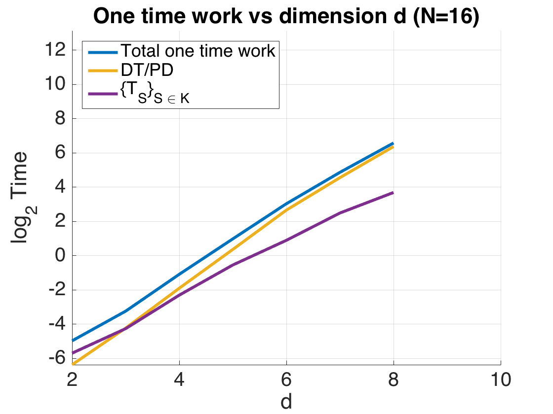
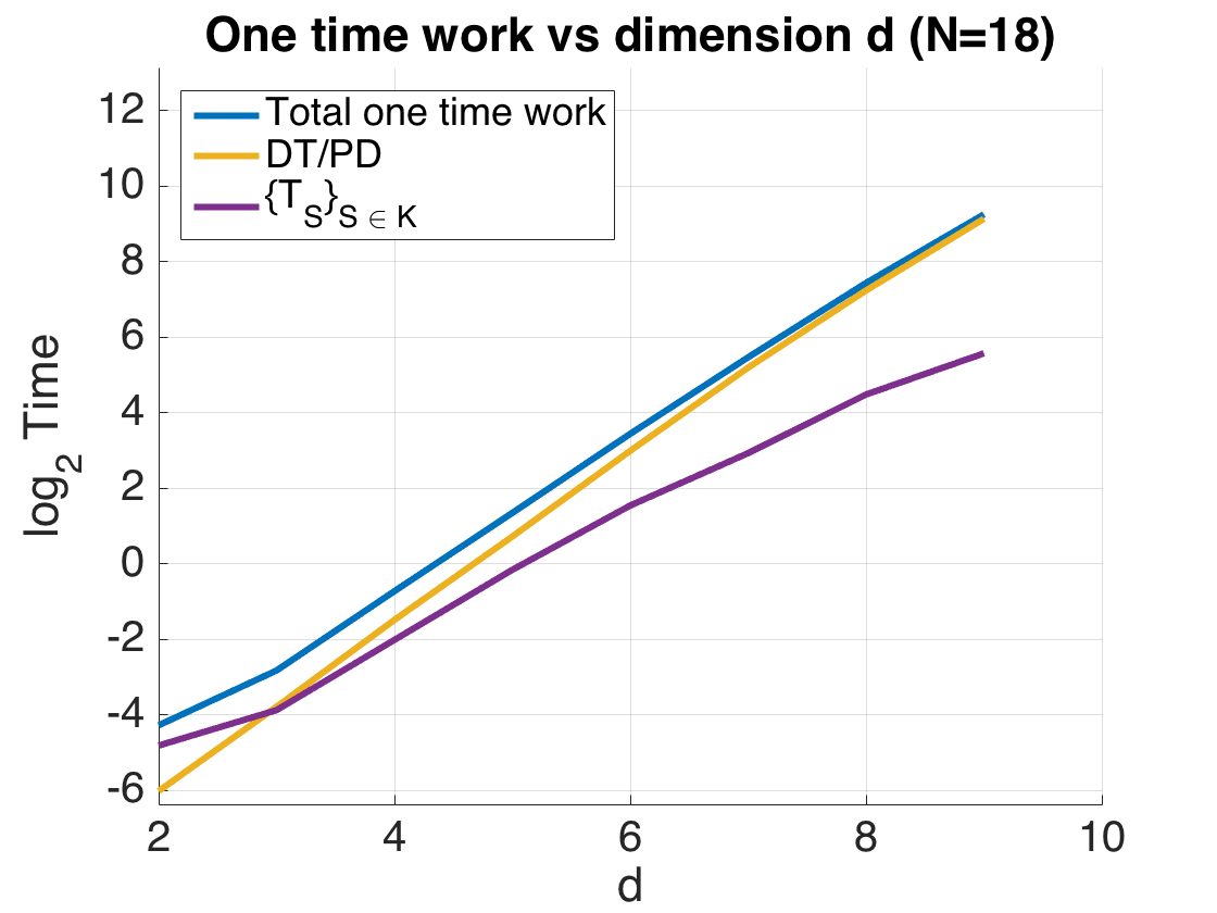
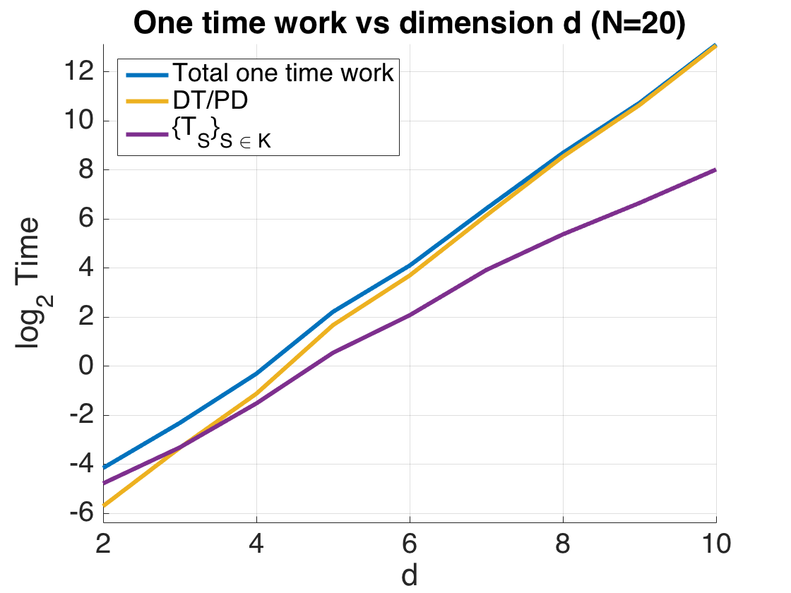
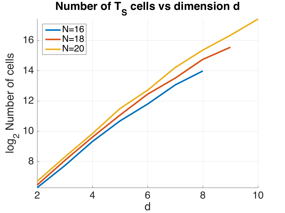
Figures 4(a), 4(b) and 4(c) show $\log_{2}$–$\log_{2}$ plots of the one time work, and its three primary components (computing $\Gamma^{1}(P;E)$, computing $\mathrm{DT}(\widetilde{E})$ / $\mathrm{PD}(\widetilde{E})$, and computing the cells $\{T_{S}\}_{S\in\mathcal{K}}$), as a function of $N$ for dimensions $d=2,3,4$. The $\log_{2}$–$\log_{2}$ plots of each of the components grow linearly, indicating that the work scales as $O(N^{\alpha})$ for some $\alpha>0$. The computation of $\Gamma^{1}(P;E)$ we know grows as $O(N^{2})$. For $d=2,3$, this component has the steepest slope, indicating that in practice the computation of the power diagram and dual triangulation, in addition to the cells $\{T_{S}\}_{S\in\mathcal{K}}$, grows as $O(N^{\alpha})$ for some $\alpha<2$. For $d=4$ however, the computation of $\mathrm{DT}(\widetilde{E})$ / $\mathrm{PD}(\widetilde{E})$ appears to grow nearly at the rate $C\cdot N^{2}$, which is the same asymptotically as the $C^{\prime}\cdot N^{2}$ growth for the computation of $\Gamma^{1}(P;E)$. However, the constant factor $C$ is significantly larger than $C^{\prime}$, which affects the practicality of the computation. We can conclude that for $d\geq 4$, the computation of the power diagram will grow at least as $O(N^{2})$, with a large constant factor independent of $N$. Figure 4(d) shows the total number of cells $\{T_{S}\}_{S\in\mathcal{K}}$ (equivalently the number of faces of $\mathrm{DT}(\widetilde{E})$ / $\mathrm{PD}(\widetilde{E})$) as a function of $N$, for $d=2,3,4$. In numerical simulations, the query work (not plotted) grew proportionally to the number of these cells.

(a) $d=2$

(b) $d=3$

(c) $d=4$

(d) $\#(\mathcal{K})$

Figure 4: One time work and number of cells $\{T_{S}\}_{S\in\mathcal{K}}$ versus $N=\#(E)$ on a $\log_{2}$–$\log_{2}$ scale, for dimensions $d=2,3,4$.

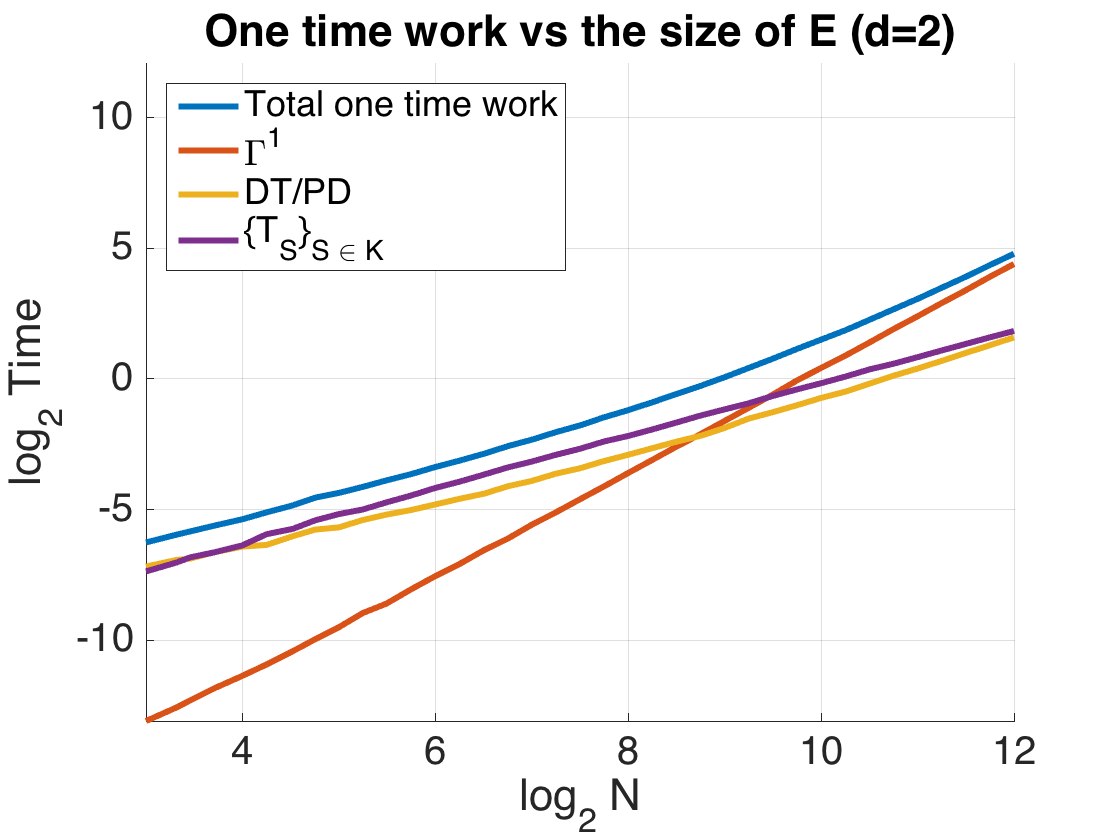
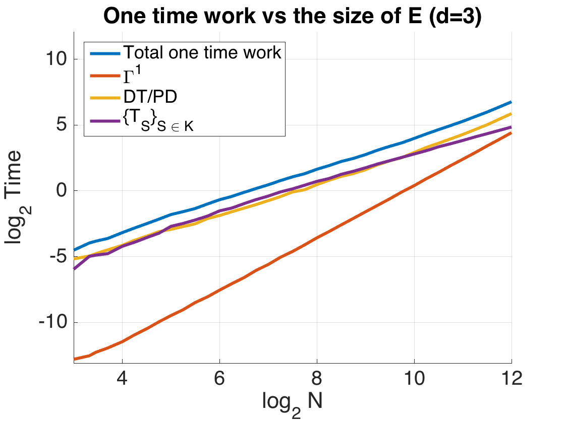
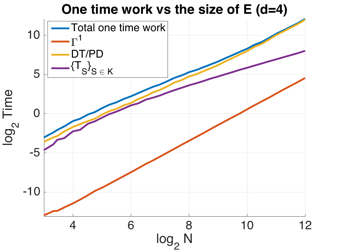
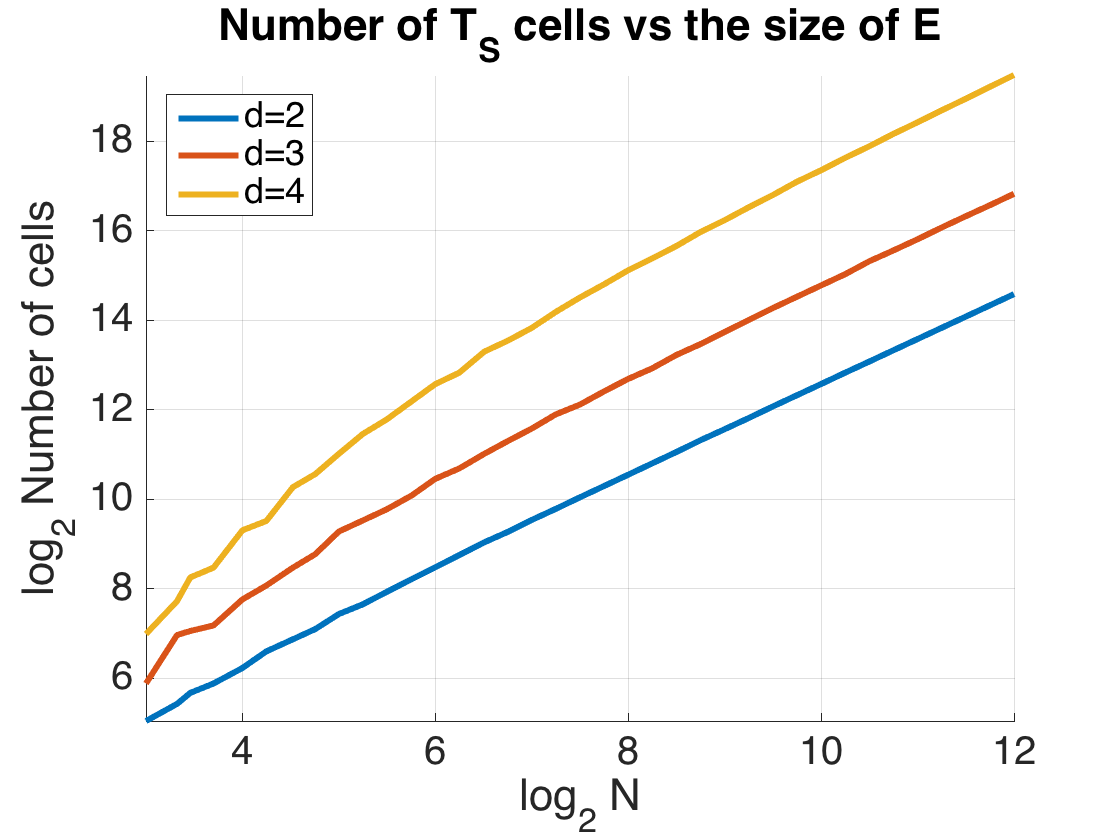
The accuracy and stability of the algorithm were tested by computing $|F(a)-f_{a}|$ and $|\partial_{x_{i}}F(a)-D_{a}f(i)|$ for each $a\in E$ and $i=1,\ldots d$. The algorithm reported an error whenever the absolute difference was more than $10^{-10}$. Across all values of $N$ tested, the number of errors for each dimension was:

• $d=2$: Function value errors: $0/25701$; Partial derivative errors: $9/51402$.

• $d=3$: Function value errors: $10/25701$; Partial derivative errors: $30/77103$.

• $d=4$: Function value errors: $3/25701$; Partial derivative errors: $12/102804$.

Thus across dimensions $d=2,3,4$, the interpolation algorithm made an error only 0.0208% of the time.

We plot the logarithm of the one time work against the dimension $d$, for a fixed size $E$, with $N=16$, $18$ and $20$ in Figures 5(a), 5(b) and 5(c), respectively. Figure 5(d) plots $\log_{2}\#(\mathcal{K})$ against the dimension $d$. Notice that all four graphs are linear. If numerically $\#(\mathcal{K})=O(N^{C_{\mathcal{K}}d})$ holds, then we should be able to solve for a consistent value of $C_{\mathcal{K}}$ from the three plots in Figure 5(d), using $\frac{\log_{2}\#(\mathcal{K})}{d}=C_{\mathcal{K}}\log_{2}N$. We estimate the slopes $\frac{\log_{2}\#(\mathcal{K})}{d}$ using a least squares fit, and then solve for $C_{\mathcal{K}}$, obtaining $C_{\mathcal{K}}=0.3241,0.3149,0.3117$ for $N=16,18,20$, respectively. Thus, for these experiments, we obtain $C_{\mathcal{K}}\approx 0.3169$. For the one time work, the computation of $\mathrm{PD}(\widetilde{E})$ / $\mathrm{DT}(\widetilde{E})$ dominates as $d$ increases. We have the similar hypothesis that the cost of this computation is $O(N^{C_{\mathrm{PD}}d})$, and for $N=16,18,20$ estimate that $C_{\mathrm{PD}}=0.5389,0.5240,0.5433$, respectively. Thus $C_{\mathrm{PD}}\approx 0.5354$ for this collection of numerical simulations. Recall from Section 5.1 that the theoretical bound for the number of cells is $\#(\mathcal{K})=O(N^{\lceil d/2\rceil})$, while the cost of computing the relevant data structures to hold $\mathrm{DT}(\widetilde{E})$ / $\mathrm{PD}(\widetilde{E})$ was $O(N^{d+1})$. From this limited collection of numerical experiments, one might hypothesize for uniformly sampled data an expected number of cells growing as $\#(\mathcal{K})\approx O(N^{d/3})$ and a one time work cost that is approximately $O(N^{d/2})$.

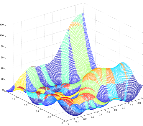
Figure 6 contains a plot of an extension colored according to the cells $\{T_{S}\}_{S\in\mathcal{K}}$.

(a) $N=16$

(b) $N=18$

(c) $N=20$

(d) $\#(\mathcal{K})$

Figure 5: The logarithm (base $2$) of the one time work and $\log_{2}\#\{T_{S}\}_{S\in\mathcal{K}}$ versus the dimension $d$, for $N=16,18,20$.

Figure 6: Interpolant $F\in C^{1,1}(\mathbb{R}^{2})$ colored by the cells $\{T_{S}\}_{S\in\mathcal{K}}$.

8 Conclusion

We introduced an efficient, practical algorithm for computing interpolations of data, consisting of a set $E\subset\mathbb{R}^{d}$ and either a $1$-field $P:E\rightarrow\mathcal{P}$ or a function $f:E\rightarrow\mathbb{R}$, with functions $F\in C^{1,1}(\mathbb{R}^{d})$ such that $\mathrm{Lip}(\nabla F)$ is within a dimensionless factor of being minimal. Amongst Whitney type interpolation algorithms, it is the first algorithm to be implemented on a computer, thus moving the development of these algorithms from theoretical constructs to proof of concept. Numerical experiments indicate that the algorithm run time is reasonable up to dimension $d=10$ for small sets $E$, as well as for larger sized initial data in small dimensions.

Fundamentally, the algorithm is built upon two key components: (1) the theoretical results of Wells [40] and Le Gruyer [33], giving a construction of the interpolant $F$ and a closed form solution for the minimal value of $\mathrm{Lip}(\nabla F)$, respectively; and (2) a collection of notions and algorithms from computational geometry, including the well separated pairs decomposition [12], power diagrams, triangulations, and convex hulls, which are used to compute the relevant values, underlying structures, and ultimately the interpolant $F$.

These results are opening new mathematical avenues related to Whitney’s extension theorem, both pure and applied. High dimensional data is being collected on an unprecedented scale; thus efficiency in both the size of $E$ and the dimension $d$ is needed. Can the efficiency of the algorithm be improved, while maintaining its precision? Notions related to approximate Voronoi diagrams [27] may be of use here, if the interpolant construction is stable. Looking further ahead, an algorithm of this type for $C^{2,1}(\mathbb{R}^{d})$ would first require results analogous to those of Wells and Le Gruyer, pertaining to precise formulations of the best Whitney’s constant. Positive results along these lines and others have the potential to push Whitney interpolation algorithms beyond proof of concept and into the applied sciences.

9 Acknowledgements

M.H. would like to thank Charles Fefferman for introducing him to the problem as well as for several helpful conservations. He would also like to thank Erwan Le Gruyer and Hariharan Narayanan for numerous insightful discussions.

All three authors would like to thank the anonymous referee whose numerous corrections, suggestions, and insights greatly improved the manuscript.

Appendix A Convex optimization

Everything in this Appendix can be found in [11]; we have summarized the parts relevant to Section 4.2 to serve as a convenient reference.

A.1 Self-concordant functions

A convex function $h:\mathbb{R}\rightarrow\mathbb{R}$ is said to be self-concordant if

$$|h^{(3)}(x)|\leq 2h^{(2)}(x)^{3/2},\quad\forall\,x\in\mathbb{R}.$$

If $h:\mathbb{R}^{n}\rightarrow\mathbb{R}$, then we say it is self-concordant if $\tilde{h}(t)=h(x+tv)$ is self-concordant as a function of $t\in\mathbb{R}$ for all $x,v\in\mathbb{R}^{n}$.

Self-concordant functions were first introduced by Nesterov and Nemirovski [35]. They are particularly useful in convex optimization since they form a class of functions for which one can rigorously analyze the complexity of Newton’s method.

A.2 Unconstrained optimization

An unconstrained convex optimization problem is one of the form:

(A.1) $$\text{minimize}\quad h(x),$$

where $h:\mathbb{R}^{n}\rightarrow\mathbb{R}$ is convex. Unconstrained convex optimization problems can be solved via any number of descent methods.

Input: A starting point $x$.

Repeat: 1. Determine a descent direction $\Delta x$. 2. Line search: Choose a step size $t>0$. 3. Update: $x\mapsto x+t\Delta x$. Until stopping criterion is satisfied.

There are several ways to determine the descent direction. We focus on Newton’s method [11, p. 484], where $\Delta x$ is given by the Newton step:

$$\Delta x=-\nabla^{2}h(x)^{-1}\nabla h(x).$$

The line search is performed using a backtracking line search [11, p. 464].

Input: A descent direction $\Delta x$ for $h$ at $x$, $\alpha\in(0,0.5)$, $\beta\in(0,1)$.

$t=1$
While $h(x+t\Delta x)>h(x)+\alpha t\nabla h(x)\cdot\Delta x$, $t\mapsto\beta t$.

Each iteration of Newton’s method is often times referred to as a Newton step, even though it entails both computing the Newton step and performing the line search.

A.3 Constrained optimization

A constrained convex optimization problem is of the form:

(A.2) minimize $$\quad h_{0}(x)$$

subject to $$\quad h_{i}(x)\leq 0,\quad i=1,\ldots,m,$$

where the functions $h_{0},\ldots,h_{m}:\mathbb{R}^{n}\rightarrow\mathbb{R}$ are convex. The function $h_{0}$ is the objective, while the functions $h_{1},\ldots,h_{m}$ are the constraints. One can solve (A.2) using interior point methods.

Define $\phi:\mathbb{R}^{n}\rightarrow\mathbb{R}$ as

$$\phi(x)=-\sum_{i=1}^{m}\log(-h_{i}(x)).$$

The following unconstrained optimization problem is closely related to (A.2),

(A.3) $$\text{minimize}\quad th_{0}(x)+\phi(x),$$

where $t>0$. Indeed, (A.3) is an approximation for our original constrained convex optimization problem, and as $t\rightarrow\infty$ the two problems become equivalent.

The barrier method [11, p. 569] solves (A.2) by iteratively solving (A.3) for increasing values of $t$, using the minimizer of one iteration as the starting point for the next iteration. Let $x^{\star}(t)$ be the minimizer of (A.3). A point $x$ is strictly feasible if $h_{i}(x)<0$ for all $i=1,\ldots,m$. The barrier method is then given as:

Input: A strictly feasible $x$, $t=t^{(0)}>0$, $\mu>1$, $\epsilon>0$

Repeat: 1. Centering step: Compute $x^{\star}(t)$ by minimizing $th_{0}+\phi$ starting at $x$. 2. Update: $x\mapsto x^{\star}(t)$. 3. Stopping criterion: Quit if $m/t<\epsilon$. 4. Increase $t$: $t\mapsto\mu t$.

The barrier method solves (A.2) with accuracy no worse than $\epsilon$. The centering step is performed using Newton’s method with a backtracking line search. The following theorem bounds the total number of Newton steps for the barrier method.

Theorem A.1 ([11, p. 591]).

Define the following constant:

$$C=\frac{10-4\alpha}{\alpha\beta(1-2\alpha)^{2}}+\log_{2}\log_{2}(1/\epsilon).$$

Suppose that $th_{0}+\phi$ is self-concordant and that the sublevel sets of $h_{0},\ldots,h_{m}$ are bounded. If $\mu=1+1/\sqrt{m}$, then the barrier method requires no more than

$$C\left(1+\log_{2}\left(\frac{m}{t^{(0)}\epsilon}\right)\sqrt{m}\right)$$

Newton steps to solve (A.2) to within accuracy $\epsilon$. If $x^{\star}$ is the solution to (A.2), the barrier method returns a value $\tilde{x}^{\star}$ such that $|h_{0}(x^{\star})-h_{0}(\tilde{x}^{\star})|\leq\epsilon$ and $h_{i}(\tilde{x}^{\star})\leq 0$ for each $i=1,\ldots,m$.

Remark A.2.

In particular, Theorem A.1 applies to quadratically constrained quadratic programs (QCQPs).

Remark A.3.

The barrier method requires a starting point $x$ that is strictly feasible. In general this requires solving for $x$, but we are only interested in convex problems of the form

minimize $$\quad s$$

subject to $$\quad h_{i}(x)\leq s,\quad i=1,\ldots,m.$$

For this type of problem, finding a strictly feasible starting point is simple. Indeed, $(x,s)\in\mathbb{R}^{n}\times\mathbb{R}$ is strictly feasible so long as $s>\max_{i=1,\ldots,m}h_{i}(x)$.

The cost per iteration of Newton’s method is the cost of computing the Newton step plus the cost of the line search. Usually the cost of the Newton step dominates. To compute the Newton step of a general unconstrained convex optimization problem (A.1) requires solving the following system of equations:

(A.4) $$H\Delta x=-g,$$

where $H=\nabla^{2}h(x)$ and $g=\nabla h(x)$. Since $H$ is symmetric and positive definite, one can use the Cholesky factorization of $H$. This decomposes $H$ as $H=LL^{T}$, where $L$ is lower triangular. One then solves $Lw=-g$ by forward substitution and $L^{T}\Delta x=w$ by back substitution. If $H$ is a dense matrix with no additional structure, then the total cost of computing the Newton step is

(A.5) $$D+\frac{1}{3}n^{3}+2n^{2},$$

where $D$ is the amount of work needed to compute $H$ and $g$, $(1/3)n^{3}$ is the amount of work for the Cholesky factorization, and $2n^{2}$ is the amount of work for the both the forward and back substitution.

If $H$ is sparse, sparse Cholesky factorization can be used in which $H=PLL^{T}P^{T}$, where $P$ is a permutation matrix. The cost of the factorization depends on the sparsity pattern, but can be much lower (e.g., $O(n^{3/2})$). The cost is heavily dependent on the choice of $P$; algorithms for finding good permutation matrices are known as symbolic factorization methods. Sparsity can also be used to speed up the forward and back substitutions.

In the case of the barrier method for solving constrained optimization problems, $h=th_{0}+\phi$. In this case,

(A.6) $$H =t\nabla^{2}h_{0}(x)+\sum_{i=1}^{m}\frac{1}{h_{i}(x)^{2}}\nabla h_{i}(x)\nabla h_{i}(x)^{T}-\sum_{i=1}^{m}\frac{1}{h_{i}(x)}\nabla^{2}h_{i}(x),$$

$$g =t\nabla h_{0}(x)-\sum_{i=1}^{m}\frac{1}{h_{i}(x)}\nabla h_{i}(x).$$

The worst case complexity of the Cholesky factorization and the forward and back substitution remain the same, but we can further analyze the cost of forming $H$ and $g$. Let $D^{\prime}$ be the amount of work needed to compute $\nabla h_{i}(x)$ and $\nabla^{2}h_{i}(x)$ for all $i=0,\ldots,m$. Then

(A.7) $$D=D^{\prime}+O(mn^{2}),$$

where the $O(mn^{2})$ term results from summing all of the terms in (A.6).

A.H.V. and F.M. were participants in the 2013 Research Experience for Undergraduates (REU) at Cornell University under the supervision of M.H. During the REU program all three were supported by the National Science Foundation (NSF) grant number NSF-1156350. This paper is the result of work started during the REU. Additionally, all three attended the “$8^{\text{th}}$ Whitney Problems Workshop,” supported by and hosted at the Centre International de Rencontres Mathématiques (CIRM), during which time the paper was revised. During the writing of the manuscript M.H. was supported by European Research Council (ERC) grant InvariantClass 320959. He is currently partially supported by an Alfred P. Sloan Research Fellowship, a DARPA Young Faculty Award, and NSF grant #1620216. F.M. is supported by a National Science Foundation Graduate Research Fellowship.

References

- [1] \RMIauthorAlmansa, A., Cao, F., Gousseau, Y., and Rougé, B. \RMIpaperInterpolation of digital elevation models using AMLE and related methods \RMIjournalIEEE Transactions on Geoscience and Remote Sensing 40 (2002), no. 2, 314–325.
- [2] \RMIauthorAmato, N. and Ramos, E. \RMIpaperOn computing Voronoi diagrams by divide-prune-and-conquer In \RMIjournalProceedings of the Annual Symposium on Computational Geometry (1996), 166–175.
- [3] \RMIauthorAronsson, G. \RMIpaperHur kan en sandhög se ut? (What is the possible shape of a sandpile?) \RMIjournalNORMAT 13 (1965), 41–44.
- [4] \RMIauthorAronsson, G. \RMIpaperMinimization problems for the functional \RMIjournalArkiv för Matematik 6 (1965), 33–53.
- [5] \RMIauthorAronsson, G. \RMIpaperMinimization problems for the functional II \RMIjournalArkiv för Matematik 6 (1966), 409–431.
- [6] \RMIauthorAronsson, G. \RMIpaperExtension of functions satisfying Lipschitz conditions \RMIjournalArkiv för Matematik 6 (1967), 551–561.
- [7] \RMIauthorAronsson, G., Evans, L. and Wu, Y. \RMIpaperFast/slow diffusion and growing sandpiles \RMIjournalJournal of Differential Equations, 131 (1996), no. 2, 304–335.
- [8] \RMIauthorAurenhammer, F. \RMIpaperPower diagrams: Properties, algorithms and applications \RMIjournalSIAM Journal on Computing 16 (1987), no. 1, 78–96.
- [9] \RMIauthorAurenhammer, F. \RMIpaperVoronoi diagrams - a survey of a fundamental geometric data structure \RMIjournalACM Computing Surveys 23 (1991), no. 3, 345–405.
- [10] \RMIauthorBarber, C., Dobkin, D. and Huhdanpaa, H. \RMIpaperThe quickhull algorithm for convex hulls \RMIjournalACM Transactions on Mathematical Software 22 (1996), no. 4, 469–483.
- [11] \RMIauthorBoyd, S. and Vandenberghe, L. \RMIbookConvex Optimization Cambridge University Press, 2004.
- [12] \RMIauthorCallahan, P. and Kosaraju, S. \RMIpaperA decomposition of multidimensional point sets with applications to -nearest-neighbors and -body potential fields \RMIjournalJournal of the Association for Computing Machinery 42 (1995), no. 1, 67–90.
- [13] \RMIauthorCaselles, V., Morel, J.M. and Sbert, C. \RMIpaperAn axiomatic approach to image interpolation \RMIjournalIEEE Transactions on Image Processing 7 (1998), no. 3, 376–386.
- [14] \RMIauthorChan, T., Snoeyink, J. and Yap, C.K. \RMIpaperOutput-sensitive construction of polytopes in four dimensions and clipped Voronoi diagrams in three In \RMIjournalProceedings of the Annual ACM-SIAM Symposium on Discrete Algorithms (1995), 282–291.
- [15] \RMIauthorChazelle, B. \RMIpaperAn optimal convex hull algorithm in any fixed dimension \RMIjournalDiscrete and Computational Geometry 10 (1993), 377–409.
- [16] \RMIauthorClarkson, K. and Shor, P. \RMIpaperApplications of random sampling in computational geometry, II \RMIjournalDiscrete and Computational Geometry 4 (1989), 387–421.
- [17] \RMIauthorDwyer, R. \RMIpaperOn the convex hull of random points in a polytope \RMIjournalJournal of Applied Probability (1988), 688–699.
- [18] \RMIauthorFavard, J. \RMIpaperSur l’interpolation \RMIjournalJournal de mathématiques pures et appliquées 19 (1940), 281–306.
- [19] \RMIauthorFefferman, C. \RMIpaperInterpolation by linear programming I \RMIjournalDiscrete and Continuous Dynamical Systems 30 (2011), no. 2, 477–492.
- [20] \RMIauthorFefferman, C., Israel, A. and Luli, G. \RMIpaperFitting a Sobolev function to data I \RMIjournalRevista Matemática Iberoamericana 32 (2016), no. 1, 275–376.
- [21] \RMIauthorFefferman, C. and Klartag, B. \RMIpaperFitting a -smooth function to data I \RMIjournalAnnals of Mathematics 169 (2009), no. 1, 315–346.
- [22] \RMIauthorFefferman, C. and Klartag, B. \RMIpaperFitting a -smooth function to data II \RMIjournalRevista Matemática Iberoamericana 25 (2009), no. 1, 49–273.
- [23] \RMIauthorFuchs, A., Jones, C. and Morari, M. \RMIpaperOptimized decision trees for point location in polytopic data sets - application to explicit MPC In \RMIjournalProceedings of the American Control Conference (2010), 5507–5512.
- [24] \RMIauthorGlaeser, G. \RMIpaperProlongement extrémal de fonctions différentiables d’une variable \RMIjournalJournal of Approximation Theory 8 (1973), 249–261.
- [25] \RMIauthorGlass, J. \RMIpaperSmooth-curve interpolation: A generalized spline-fit procedure \RMIjournalBIT Numerical Mathematics 6 (1966), no. 4, 277–293.
- [26] \RMIauthorLe Gruyer, E. and Phan, T.V. \RMIpaperSup-Inf explicit formulas for minimal Lipschitz extensions for 1-fields on \RMIjournalJournal of Mathematical Analysis and Applications 424 (2015), no. 2, 1161–-1185.
- [27] \RMIauthorHar-Peled, S. \RMIpaperA replacement for voronoi diagrams of near linear size In \RMIjournalProceedings of the 42nd IEEE Symposium on Foundations of Computer Science (FOCS’01) (2001).
- [28] \RMIauthorHirn, M. and Le Gruyer, E. \RMIpaperA general theorem of existence of quasi absolutely minimal Lipschitz extensions \RMIjournalMathematische Annalen 359 (2014), no. 3–4, 595–628.
- [29] \RMIauthorHolladay, J. \RMIpaperA smoothest curve approximation \RMIjournalMathematics of Computation 11 (1957), 233–243.
- [30] \RMIauthorJensen, R. \RMIpaperUniqueness of Lipschitz extensions: Minimizing the sup norm of the gradient \RMIjournalArchive for Rational Mechanics and Analysis 123 (1993), no. 1, 51–74.
- [31] \RMIauthorKirszbraun, M. \RMIpaperÜber die zusammenziehende und Lipschitzsche Transformationen \RMIjournalFundamenta Mathematicae 22 (1934), 77–108.
- [32] \RMIauthorKyng, R., Rao, A., Sachdeva, S. and Spielman, D. \RMIpaperAlgorithms for Lipschitz learning on graphs \RMIjournalJMLR: Workshop and Conference Proceedings 40 (2015), 1–34.
- [33] \RMIauthorLe Gruyer, E. \RMIpaperMinimal Lipschitz extensions to differentiable functions defined on a Hilbert space \RMIjournalGeometric and Functional Analysis 19 (2009), 1101–1118.
- [34] \RMIauthorLipton, R., Rose, D. and Tarjan, R. \RMIpaperGeneralized nested dissection \RMIjournalSIAM Journal on Numerical Analysis 16 (1979), no. 2, 346–358.
- [35] \RMIauthorNesterov, Y. and Nemirovskii, A. \RMIbookInterior-Point Polynomial Methods in Convex Programming Society for Industrial and Applied Mathematics, 1994.
- [36] \RMIauthorPeres, Y., Schramm, O., Sheffield, S. and Wilson, D. \RMIpaperTug-of-war and the infinity Laplacian \RMIjournalJournal of the American Mathematical Society 22 (2009), no. 1, 167–210.
- [37] \RMIauthorSeidel, R. \RMIpaperConstructing high-dimensional convex hulls at logarithmic cost per face In \RMIjournalProceedings of the Annual ACM Symposium on Theory of Computing (1986), 404–413.
- [38] \RMIauthorSeidel, R. \RMIpaperSmall-dimensional linear programming and convex hulls made easy \RMIjournalDiscrete and Computational Geometry 6 (1991), 423–434.
- [39] \RMIauthorTondel, P., Johansen, T. and Bemporad, A. \RMIpaperEvaluation of piecewise affine control via binary search tree \RMIjournalAutomatica 39 (2003), 945–950.
- [40] \RMIauthorWells, J. \RMIpaperDifferentiable functions on Banach spaces with Lipschitz derivatives \RMIjournalJournal of Differential Geometry 8 (1973), 135–152.
- [41] \RMIauthorWhitney, H. \RMIpaperAnalytic extensions of differentiable functions defined in closed sets \RMIjournalTransactions of the American Mathematical Society 36 (1934), no. 1, 63–89.