First-principles calculations of phonon frequencies, lifetimes and spectral functions from weak to strong anharmonicity: the example of palladium hydrides
Abstract
The variational stochastic self-consistent harmonic approximation is combined with the calculation of third-order anharmonic coefficients within density-functional perturbation theory and the “” theorem to calculate anharmonic properties of crystals. It is demonstrated that in the perturbative limit the combination of these two methods yields the perturbative phonon linewidth and frequency shift in a very efficient way, avoiding the explicit calculation of fourth-order anharmonic coefficients. Moreover, it also allows calculating phonon lifetimes and inelastic neutron scattering spectra in solids where the harmonic approximation breaks down and a non-perturbative approach is required to deal with anharmonicity. To validate our approach, we calculate the anharmonic phonon linewidth in the strongly anharmonic palladium hydrides. We show that due to the large anharmonicity of hydrogen optical modes the inelastic neutron scattering spectra are not characterized by a Lorentzian line-shape, but by a complex structure including satellite peaks.
I Introduction
Anharmonic effects are responsible for the finiteness of the phonon lifetimes observed experimentally as well as the temperature dependence of the phonon frequencies. Indeed, harmonic phonon frequencies are temperature independent and, as not decaying quasiparticles, harmonic phonons’ lifetime is infinite, yielding an artificial infinite value for the thermal conductivity. Considering that the calculation of the lattice thermal conductivity is crucial in semiconducting thermoelectrics Mahan et al. (1997); DiSalvo (1999) and in materials used for thermal dissipation Cahill et al. (2003), the development of precise and reliable ab initio approaches based on density-functional theory (DFT) to calculate anharmonic effects, including the calculation of lifetimes, is currently a strongly active field of research.
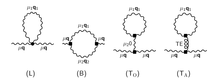
Anharmonic effects can be treated perturbatively as long as they are weak. At lowest order, the harmonic phonon self-energy should be corrected by the four Feynman self-energy diagrams represented in Fig. 1 Maradudin and Fein (1962); Calandra et al. (2007). The real part of the diagrams contributes to the phonon lineshift, i.e., to a change of the phonon frequency, while the imaginary part of the diagrams is responsible for the broadening of phonon lines. The three phonon process described by the bubble diagram contributes to both the linewidth and the lineshift, while the loop diagram has a two-phonon fourth-order vertex which contributes exclusively to the lineshift. We have finally decomposed the tadpole diagram in an optical part (TO), which contributes to the relaxation of internal coordinates, and an acoustical part (TA), where the line of zero energy and momentum can be associated to the elastic constants of the material and accounts for the thermal expansion. The tadpole diagrams reduce to the quasi-harmonic approximation (QHA) under certain conditions Lazzeri and de Gironcoli (1998).
The summation of these diagrams ab initio requires the knowledge of third- and fourth-order derivatives of the Born-Oppenheimer (BO) total energy. During the last 20 years several implementations have emerged to efficiently compute the third-order derivatives via the “” theorem Gonze and Vigneron (1989); Debernardi et al. (1995); Lazzeri and de Gironcoli (2002); Deinzer et al. (2003); Paulatto et al. (2013). On the contrary, the fourth order term cannot be computed in this framework, but it can be obtained by finite difference calculations of the third-order diagrams. As the number of fourth-order derivatives quickly increases with the number of atoms, the perturbative evaluation of the loop diagram is only affordable for few atoms highly symmetric cells Bonini et al. (2007). Thus, new approaches to calculate fourth-order terms from first-principles are highly desirable. Despite such difficulties, the perturbative approach has been successfully exploited in many different applications, ranging from computing phonon lifetimes Lazzeri and de Gironcoli (1998); Shukla et al. (2003) and mean free paths Paulatto et al. (2013), to thermal expansion Lazzeri and de Gironcoli (2002) and thermal conductivity of materials in the single mode approximation Broido and Reinecke (2004); *Broido05; *Ward09; Paulatto et al. (2013) or solving exactly the Boltzmann transport equation Fugallo et al. (2013).
On the other hand, the perturbative approach to anharmonicity is built on top of a harmonic description of the material and it breaks down when the harmonic model does. For instance when a material exhibits imaginary phonon frequencies, either because of a real mechanical instability or because the phase is stabilized by quantum or thermal fluctuations strongly affected by the anharmonic potential. This is the case in many ferroelectrics Zhong et al. (1995); Yu and Krakauer (1995) and thermoelectrics Delaire et al. (2011); Li et al. (2014). In systems with light atomic species, the large amplitude rattling vibrations can also make the harmonic approximation break down Rousseau and Bergara (2010); Liu and Ma (2013). Even the presence of soft modes associated with charge-density waves Leroux et al. (2012); Calandra et al. (2009); Calandra and Mauri (2011); Johannes and Mazin (2008); Johannes et al. (2006) can invalidate assumptions of perturbative methods. Calculating phonon lifetimes and, consequently, the thermal conductivity in all these systems requires, therefore, going beyond the perturbative approach.
In this work we want to tackle these problems by combining the third-order perturbative approach, which provides the leading order contribution to the phonon line broadening, with the stochastic self-sonsistent harmonic approximation (SSCHA) method Errea et al. (2013, 2014), which is based on a variational approach and gives an accurate description of the phonon spectra in the non-perturbative regime. We show that for small anharmonicity the combination of these methods accounts for all the diagrams in Fig. 1 yielding the correct perturbative limit. Thus, the perturbative correction can be obtained avoiding the cumbersome and expensive calculation of fourth-order force-constants. In fact, in this limit, the SSCHA accounts for TO and TA tadpole diagrams as well as the loop diagram, while the bubble diagram is computed making use of the third-order force-constants calculated with the “” theorem over the whole Brillouin Zone (BZ) Paulatto et al. (2013). In the non-perturbative regime, combining the SSCHA equilibrium positions, phonon frequencies and polarization vectors with the calculated third-order coefficients, phonon lifetimes and spectral functions can be obtained for strongly anharmonic crystals where the harmonic approximation breaks down.
We apply this method to palladium hydride stoichiometric compounds: PdH, PdD and PdT. Because of the huge anharmonicity of hydrogen rattling vibrations the phonon dispersions predicted by density-functional perturbation theory (DFPT) show strong instabilities and a huge underestimation of the H-character optical modes. The instabilities are even more pronounced at finite temperature when the thermal expansion is considered. These instabilities are however not physical and can be cured with the SSCHA approach, which yields phonon spectra in good agreement with experiments Errea et al. (2013, 2014). The anharmonicity also causes an interesting negative superconducting isotope coefficient Errea et al. (2013). Here we find that, despite being a metal, the phonon linewidth is dominated by the phonon-phonon interaction for any temperature above a few Kelvin. The third-order broadening of the phonon modes is huge, at the point that the simplistic model of well-distinct phonon modes, broadened to a finite-width Lorentzian function, cannot be applied anymore. It is remarkable, however, that the phonon shift induced by the third-order is not predominant over the SSCHA correction of the phonon bands.
II The ionic Hamiltonian: phonon anharmonicity and the electron-phonon coupling
Within the BO approximation, the dynamics of the ions in a crystalline solid are determined by the following Hamiltonian:
| (1) |
where
| (2) |
is the kinetic-energy operator of the ions and the potential defined by the BO energy surface. Let denote an ion within the unit cell, a lattice vector and a Cartesian direction. In the equation above is the momentum operator and the mass of ion . Considering that generally ions vibrate around their equilibrium position determined by the minima of the BO energy surface, the potential is Taylor-expanded as a function of the ionic displacements from equilibrium as
| (3) |
where
| (4) |
and
| (5) |
represents the -th order derivative of the BO energy surface with respect to the atomic displacements calculated at equilibrium, namely, the -th order, or -bodies, force-constants.
The Hamiltonian in Eq. (1) represents a complicated many-body problem, unsolvable unless an approximated scheme is adopted.
II.1 The harmonic approximation
The first non-trivial approximation is the harmonic approximation, in which the expansion in Eq. (3) is truncated at second order. In Fourier space the Hamiltonian looks like
| (6) |
If the phonon frequencies and polarizations diagonalize the dynamical matrix at momentum ,
| (7) |
by applying the following change of variables
| (8) | |||||
| (9) |
can be written in this well-known diagonal form:
| (10) |
Here and are, respectively, the phonon creation and annihilation operators. Thus, if the ionic Hamiltonian is approximated by , phonons are well-defined quasiparticles that do not interact nor decay.
II.2 Anharmonic effects and perturbation theory
It is convenient to write the Hamiltonian in Fourier space as Calandra et al. (2007)
| (11) | |||||
where . The reader is referred to Appendix A for the definition of the high-order anharmonic coefficients. Due to translational symmetry, for each coefficient crystal momentum is conserved so that , where is a reciprocal lattice vector Rousseau and Bergara (2010).
Within perturbation theory, the lowest energy corrections to the harmonic non-interacting phonon propagator are given by the loop (L), bubble (B) and tadpole (T) self-energy diagrams shown in Fig. 1. Their contribution to the self-energy are given by Maradudin and Fein (1962); Rousseau and Bergara (2010); Calandra et al. (2007); Lazzeri et al. (2003)
| (12) | ||||
| (13) | ||||
| (14) |
where
| (15) |
is the bosonic occupation factor and the number of unit cells in the system. Thus,
| (16) |
is the total self-energy at the perturbative level.
The tadpole TO diagram includes an optical phonon at the point () and it accounts for the relaxation of internal coordinates. If internal coordinates are determined by symmetry, it vanishes and does not contribute Maradudin and Fein (1962); Calandra et al. (2007); Lazzeri et al. (2003). On the contrary, if Wyckoff’s positions have free parameters, the TO diagram accounts for the effect of quantum and thermal fluctuations in the internal coordinates. Its effect can be accounted if internal coordinates are those that minimize the QHA free energy. For those internal coordinates, the TO self-energy vanishes. These equilibrium positions might differ from the positions derived from the minima of the BO energy surface. The related TA diagram includes the limit for of an acoustical phonon, and accounts for the relaxation of the cell parameters. It can also be calculated within the QHA Bonini et al. (2007).
The bubble contribution is the only self-energy term with an imaginary part. Thus, it is the only one contributing to the phonon linewidth. As long as , the half-width at half-maximum (HWHM) of phonon with momentum is given by the imaginary part of the bubble self-energy term at the harmonic frequency, namely,
| (17) |
The shift of the harmonic frequency due to the phonon-phonon interaction is given instead by the real part of both loop and bubble diagrams,
| (18) |
The frequency shifted by anharmonicity is thus .
II.3 The non-perturbative limit and the stochastic self-consistent harmonic approximation
The perturbative scheme introduced in Sec. II.2 assumes that phonons can be described as well-distinct quasi-particle states. This assumption is only valid when the anharmonic self-energy is small with respect to the separation between harmonic frequencies. If is comparable to or larger than , it breaks down and the phonon linewidhts and shifts derived from Eqs. (17) and (18) are not correct. In case the system has harmonic imaginary frequencies, i.e., it is unstable in the harmonic approximation, the perturbative approach cannot even be applied.
A useful workaround that allows treating this non-perturbative regime is the variational approach defined by the self-consistent harmonic approximation (SCHA) Hooton (1955), which has been recently implemented in a stochastic framework within the SSCHA Errea et al. (2013, 2014). The exact vibrational free energy of a solid is given by the sum of the total energy and the entropy:
| (19) |
where the is the density matrix and . In the SSCHA is substituted by a trial density matrix defined by a trial Hamiltonian. Then, if
| (20) |
we have the
| (21) |
variational equation. Thus, minimizing with respect to the trial Hamiltonian a good approximation of the free energy is obtained.
Even if the variational principle in Eq. (21) is valid for any trial potential , in the SSCHA we assume that is a harmonic potential that can be parametrized as
| (22) |
The atomic displacements are different from the displacements. The latter measure the displacement of the atoms from , while the first represent the displacement from trial equilibrium positions, . Similarly the force-constants are not the harmonic ones of Eq. (6), but some trial force-constants. Thus, the independent parameters in are simply and . In the SSCHA is minimized with respect to these parameters making use of a conjugate-gradient (CG) algorithm. During the minimization crystal symmetries are preserved. At the minimum, the positions are the equilibrium positions including anharmonic effects and the phonon frequencies and polarizations obtained diagonalizing yield the phonon spectra renormalized by anharmonicity.
The gradient of needed for the CG minimization is given in Fourier space by Errea et al. (2013, 2014)
| (23) | |||
| (24) |
where represents the quantum statistical average calculated with . In Eqs. (23) and (24) is the vector formed by all the atomic forces at momentum and denotes the vector formed by the forces derived from . The normal length is , and and are different from the harmonic phonon frequencies and polarizations since they are obtained diagonalizing and not . In the SSCHA the quantum statistical averages in Eqs. (23) and (24) are calculated stochastically calculating atomic forces on supercells with ionic configurations described by , where represents a general ionic configuration Errea et al. (2013, 2014).
II.4 Combining the SSCHA with the perturbative expansion
The internal coordinates determined by the SSCHA are those that make the quantum statistical average of the forces on the ions vanish. As shown in Appendix B, in the perturbative limit this means that the TO diagram vanishes for those coordinates. The reason is that the tadpole diagram includes the term, which vanishes if the quantum statistical average of the forces is zero. The TA diagram that describes the thermal expansion is also included in the SSCHA if the lattice parameters are determined by the minima of the free energy Errea et al. (2014). Therefore, in the perturbative limit the SSCHA reduces to the QHA.
On the other hand, we also show in Appendix B that for a fixed cell geometry the perturbative limit of the frequency shift given by the SSCHA is exactly the shift given by the loop self-energy term. Therefore, the SSCHA provides a stochastic framework to calculate the fourth-order anharmonic shift in systems were perturbation theory works. This is very remarkable as with the SSCHA we avoid the cumbersome and time-demanding calculation of anharmonic coefficients needed in Eq. (12), which are usually calculated taking first-order numerical derivatives of third-order anharmonic terms or second-order numerical derivatives of dynamical matrices calculated in supercells Lang et al. (1999); Lazzeri et al. (2003); Rousseau and Bergara (2010); Errea et al. (2011, 2012); Bonini et al. (2007). This result also indicates that in the perturbative limit the SSCHA does not include the bubble self-energy. Notwithstanding that, it shows us that the bubble self-energy can be included on top of the SSCHA result.
Once the minimization procedure of the SSCHA has been performed, the difference between the SSCHA and the exact potential is lead by the third-order term: . The lowest-energy third-order contribution to the self-energy is obtained by substituting the SSCHA equilibrium positions, phonon frequencies and polarizations in Eq. (13),
| (25) |
where the superscript denotes that the anharmonic coefficients and the self-energy are calculated with the SSCHA equilibrium positions, phonon frequencies and polarizations (see Appendix A). Then, the linewidth is and the SSCHA phonon frequencies can be corrected with the shift. In the perturbative limit, when , the bubble self-energy in Eq. (25) trivially reduces to the perturbative one in Eq. (13). As the SSCHA includes both the tadpole and loop self-energy corrections, including this third-order contribution yields the correct perturbative limit. In the non-perturbative limit on the contrary, we assume that the lowest-energy correction to the SSCHA result is dominated by Eq. (25). This type of “bubble” correction to the SCHA phonon frequencies was already applied by Cowley using a model potential for a point mode of a diatomic ferroelectric Cowley (1996). This framework, therefore, allows us to calculate not only bubble self-energy corrections to the SSCHA result, but to calculate anharmonic lifetimes in strongly anharmonic systems, opening the door to the calculation of the thermal conductivity in crystals were the perturbative expansion breaks down.
II.5 The electron-phonon linewidth
For metals the phonons acquire an additional linewidth contribution due to the electron-phonon interaction. In complete analogy with the anharmonic case, the phonon linewidth associated to the electron-phonon interaction is given by the imaginary part of the phonon self-energy associated to the electron-phonon interaction. Within Migdal’s lowest-order approximation for the self-energy, the linewidth at HWHM reads Allen and Mitrovic (1982); Calandra and Mauri (2005)
| (26) | |||||
In Eq. (26), is the electron-phonon matrix element, a Kohn-Sham state with energy measured from the Fermi energy, is a normal coordinate, and is the Fermi-Dirac distribution function for state . Considering the large value of the Fermi energy compared to the phonon frequencies, the temperature dependence of is very weak and the sum in Eq. (26) is usually restricted to the states at the Fermi surface Allen (1972):
| (27) |
In this work we assume that the electron-phonon linewidth is temperature independent and it will be calculated making use of Eq. (27).
As it can be noted from Eq. (27), is independent of the phonon frequency. However, it depends on the phonon polarization vectors. If perturbation theory breaks down, the harmonic polarization vectors might not be correct, yielding to a wrong linewidth. This problem is overcome substituting in Eq. (27) the harmonic polarization vectors with the SSCHA polarization vectors, allowing the calculation of electron-phonon linewidths in strongly anharmonic crystals.
| 0 K | 295 K | |||
|---|---|---|---|---|
| 1 | 0.010 | 0.000 | 0.005 | |
| 2 | 0.010 | 0.000 | 0.005 | |
| 3 | 0.136 | 0.003 | 0.198 | |
| 4 | 1.288 | 0.123 | 24.993 | |
| 5 | 1.288 | 0.123 | 24.993 | |
| 6 | 2.265 | 17.284 | 44.423 | |
| 1 | 0.142 | 0.000 | 0.012 | |
| 2 | 0.142 | 0.000 | 0.012 | |
| 3 | 0.027 | 0.006 | 0.069 | |
| 4 | 4.212 | 0.123 | 24.152 | |
| 5 | 4.121 | 0.123 | 24.152 | |
| 6 | 3.202 | 1.496 | 13.166 | |
| 1 | 0.021 | 0.000 | 0.298 | |
| 2 | 0.021 | 0.000 | 0.298 | |
| 3 | 0.025 | 0.029 | 0.518 | |
| 4 | 2.498 | 8.303 | 30.590 | |
| 5 | 2.498 | 8.303 | 30.590 | |
| 6 | 5.525 | 3.913 | 8.336 | |
III Computational details
In this work we combine the calculation of the anharmonic bubble diagram with the SSCHA as described in Sec. II.4 for palladium hydrides. All calculations are performed within DFT making use the Perdew-Zunger local-density approximation Perdew and Zunger (1981) and ultrasoft pseudopotentials. Harmonic phonon calculations are calculated within DFPT as inplemented in Quantum-ESPRESSO Giannozzi et al. (2009). We have cut off the kinetic energy of the electron wavefunctions basis set at 50 Ry, and we have used a 24 24 24 Mokhorst-Pack mesh to sample the BZ. The sum over in Eq. (27) for the electron-phonon linewidth requires a finer 72 72 72 grid.
The calculation of the third-order anharmonic coefficients is performed using the recent implementation of the “” theorem Paulatto et al. (2013) for all the triplets of points with and in a regular mesh. The remaining is determined by crystal momentum conservation. These coefficients are calculated for the equilibrium volume calculated for PdH within the SSCHA Errea et al. (2013) at 0 K. We assume that the coefficients do not change with temperature or isotope mass. The coefficients were Fourier-transformed to three-body force constants and interpolated on a finer grid of points (Appendix C, Ref. Paulatto et al., 2013). For the regularization of Eq. (15) we have used 5 cm-1, which corresponds to a Gaussian smearing of width of about 4 cm-1 if the simplified formula of Eq. (6) from Ref. Paulatto et al., 2013 is used.
The SSCHA calculations have been performed as described in Ref. Errea et al., 2013. The temperature dependence of the SSCHA dynamical matrices is estimated with the model potential described in Ref. Errea et al., 2013. The thermal expansion is taken into account using the temperature dependent lattice parameters presented in Ref. Errea et al., 2014. However, we use the model potential exclusively to calculate the temperature shift of the dynamical matrices as the zero-temperature dynamical matrices are calculated fully ab initio as in Ref. Errea et al., 2013. If the dynamical matrices are those calculated with the model potential at temperature and momentum , the temperature-induced shift of the dynamical matrices is calculated as . We add this difference to the matrices calculated fully from first-principles at 0 K, so that .
IV Results and discussion
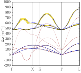
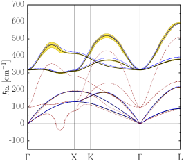
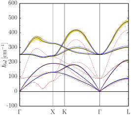
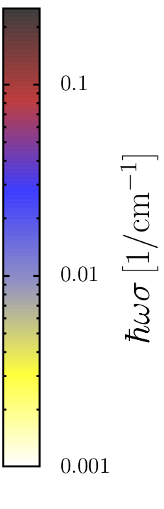
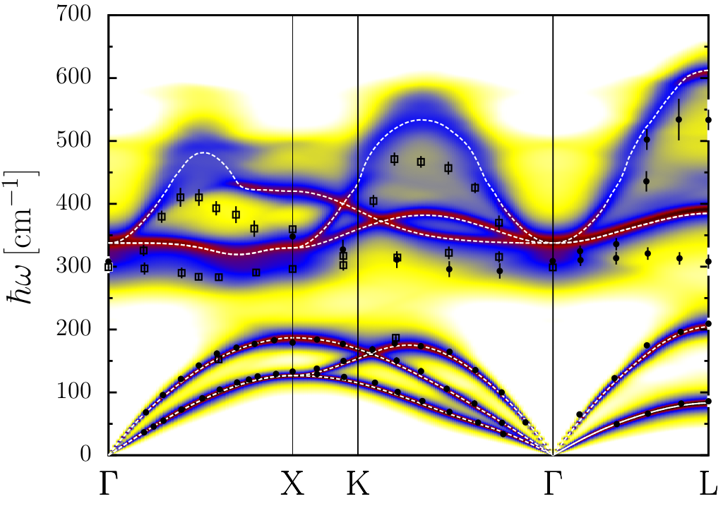
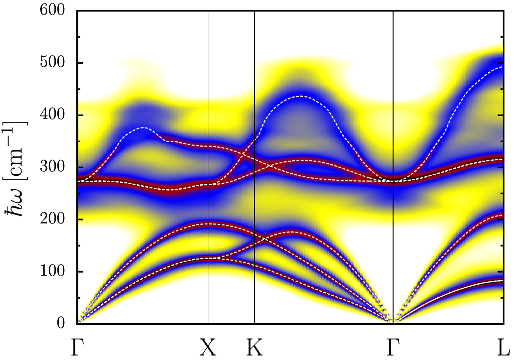
The collapse of the harmonic approximation that was discussed in Refs. Errea et al., 2013 and Errea et al., 2014 is evident in Fig. 2, where the harmonic phonon spectra is plotted both at low and high temperature. The temperature dependence of the harmonic phonon spectra comes solely from the thermal expansion. It is clear from the figure that at room temperature the phonon instabilities become much more dramatic. The H-character optical modes become unstable even at the point, and strongly mix with the Pd-character acoustic modes throughout the BZ. Considering that experimentally palladium hydrides exist even above room temperature in the rock-salt structure Flanagan (1991), the instabilities predicted in the harmonic approximation are not real, and a non-perturbative scheme like the SSCHA is required to study vibrational properties in palladium hydrides.
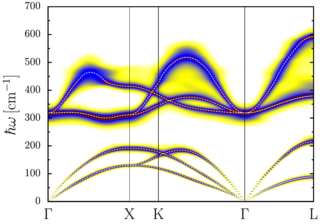
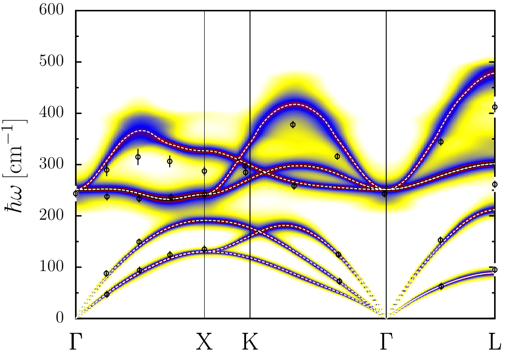
In Fig. 2 we present the SSCHA phonon spectra at 80 and 295 K, together with the SSCHA spectra shifted by calculated as described in Sec. II.4. The calculated linewidths are depicted as well. Within the SSCHA the energy of the H-character optical modes is strongly enhanced, optical and acoustic modes disentangle, and the resulting spectra is in rather good agreement with experimental results Errea et al. (2013); Rowe et al. (1974, 1986). It is remarkable that the shift introduced by the bubble diagram is very small compared to the SSCHA correction of the phonon frequency. Moreover, is small for all modes compared to the SSCHA renormalized frequencies. This is an a posteriori confirmation that the third-order term of the BO potential can be treated within perturbation theory starting from the SSCHA solution as discussed in Sec. II.4.
The calculated phonon linewidth associated to the phonon-phonon interaction is also small compared to the SSCHA phonon frequencies. This is expected as the real and imaginary parts of the phonon self-energy are related by a Kramers-Kronig integral. As a consequence, despite the huge anharmonicity, phonons in palladium hydrides are still quasiparticles that can be observed experimentally Rowe et al. (1974, 1986). This statement is still valid at high temperature, although the linewidth associated to the phonon-phonon interaction is strongly enhanced with temperature.
The values of the electron-phonon and phonon-phonon linewidths are summarized in Table 1. The linewidth is larger than for the optical H-character modes at most points even in the low-temperature regime. At 295 K the anharmonic linewidth is always larger than the electron-phonon linewidth for these modes. This is not the case for other superconducting metals, where the linewidth coming from the electron-phonon interaction is usually larger than the anharmonic linewidth Shukla et al. (2003); Rousseau and Bergara (2010). The Pd-character acoustic modes have a considerably lower anharmonic and electron-phonon linewidth, remarking that they are very harmonic and barely contribute to superconductivity Errea et al. (2013).
At low temperature, the phonon-phonon linewidth of the high-energy optical mode is larger than the linewidth of the low-energy optical mode, especially halfway along X. The reason is that the high-energy optical phonons can decay into a low-energy optical mode and a high-energy acoustic mode while conserving energy and crystal momentum. When temperature is increased and acoustic modes start to be occupied, other optic modes acquire a larger linewidth, but the one with largest linewidth is still the highest-energy optical mode at , where is the lattice parameter.
So far we have assumed that only depends on q and on the phonon band, and that it is independent of the energy. This may however be false when the phonon linewidth becomes comparable with the energy separation of non-degenerate modes. However, this is not an issue for our technique, because having the SSCHA phonon frequencies and the self-energy we can simulate the phonon spectral function at an arbitrary q-point, and without any assumption, according to the following expression:Cowley (1968)
| (28) |
Substituting in Eq. (28) and the spectral function reduces to a combination of Lorentzian functions. This substitution is justified as long as the real part of the self-energy remains constant in the energy range defined by the phonon linewidth. Indeed, in most cases the measured inelastic neutron scattering (INS) spectra show Lorentzian line-shapes Cowley (1968), as the experimental phonon frequency is determined by the position of the peak and the linewidth of the Lorentzian gives the experimental phonon linewidth.
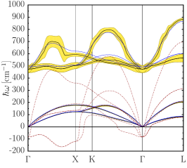
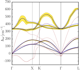
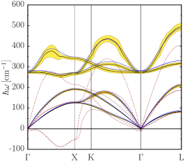
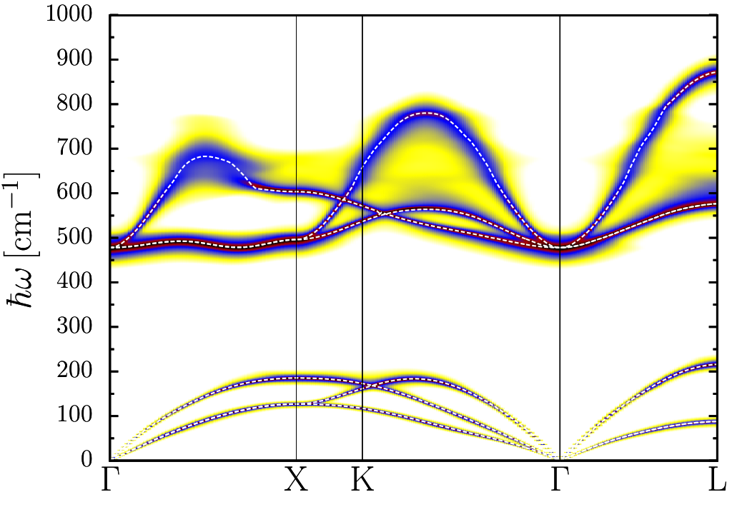
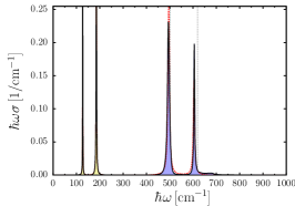
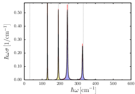
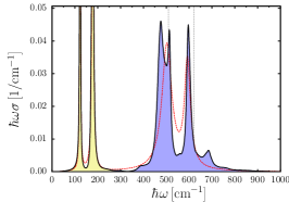
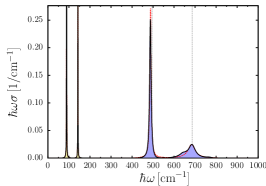
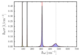
In Fig. 3 we plot the spectral function for PdH, PdD and PdT at 80 and 295 K, keeping the full dependence on of the self-energy. As it can be observed, while the acoustic phonon peaks in fulfill with the simple Lorentzian picture, the highest energy modes already at 80 K show shoulders in their peaks not expected a priori. The situation becomes more dramatic at high temperature, as shows very wide resonances with a non-Lorentzian peak at most points for the optical modes, sometimes even with satellite peaks. The reason for this is that the self-energy is not constant in the range defined by the big linewidth of the optical modes. Having satellite peaks can be very misleading for experimentalists, since they can be interpreted as structural phase transitions. However, as in the case of palladium hydrides, secondary peaks emerge due to strong anharmonicity. A similar effect has been recently reported in PbTe Delaire et al. (2011); Li et al. (2014).
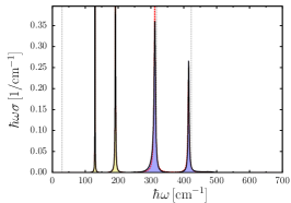
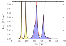
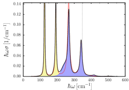
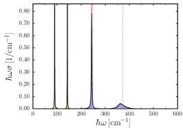
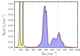
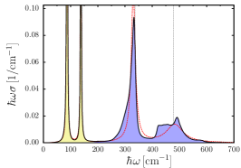
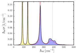
In Figs. 4 and 5 we plot for the X point and , respectively. We decided to plot multiplied by because the integral of this quantity over the entire energy domain gives the number of modes Cowley (1997). The curve obtained substituting in Eq. (28) and is also shown. It is clear from the figures that the latter approximation yields good spectral peaks for the Pd-character acoustic modes, but not for the H-character optical modes, specially at high temperature. For instance, at the X point at 295 K for PdH we observe that the peak associated to the lowest-energy optical mode is split into two distinct peaks and the highest-energy optical mode shows a satellite peak at high energy. The departure from the Lorentzian line-shape is less acute for the heavier isotopes. At on the contrary, the highest-energy optical peak appears with a complex line-shape with a double-peak structure for all the isotopes both at low and high temperature. We made the hypothesis that this complex line-shape is caused by the presence of two competing decay mechanisms; for example in the PdD case at the point we have a strong peak around 490 cm-1, which is interestingly situated higher than the energy of the unperturbed SSCHA phonon eigenvalue (479.1 cm-1). Another peak is present at a slightly lower energy, around 450 cm-1. We decomposed the contribution to at this point and the energy of the two peaks, over the BZ. We found that the higher peak is caused by the activation of a decay channel toward two phonons on the lower optical band: one at X, the other at the Gamma point. This decay mechanism is forbidden at the energy of the lower peak, where the favourite decay mechanism is toward one optical and one acoustical phonon.
Even if in INS experiments in non-stoichiometric palladium hydrides complex line-shapes with a large linewidth were observed Rowe et al. (1974, 1986), larger than those calculated by us here, the origin of the structure has been attributed to the non-stoichiometry Glinka et al. (1978). Thus, we avoid the explicit comparison with experiments as we are dealing with stoichiometric hydrides.
V Summary and conclusions
In this work we show how two different brand-new approaches can be combined to gain further insight into the anharmonic properties of solids: the non-perturbative stochastic self-consistent harmonic approximation Errea et al. (2013, 2014), which is valid to deal with strongly anharmonic crystals, and the calculation of third-order anharmonic coefficients within DFPT and the “” theorem Paulatto et al. (2013). The combination of these two methods (i) yields the correct perturbative limit for small anharmonicity and (ii) allows including self-energy corrections to the variational SSCHA result. Thus, the combination of the SSCHA with the “” theorem offers us the possibility to calculate anharmonic phonon shifts and lifetimes at any point in the BZ in a very efficient way for crystals were perturbation theory remains valid, avoiding the cumbersome calculation of fourth-order anharmonic coefficients. Moreover, it also allows calculating phonon lifetimes and INS spectra for those crystals where a non-perturbative approach of anharmonicity is required. Thus, this approach might be very appealing for calculating thermal conductivity in strongly anharmonic crystals like thermoelectrics.
The combination of the SSCHA and the “” theorem is applied to the strongly anharmonic palladium hydrides, where the harmonic theory completely breaks down. We show that despite being a superconducting metal the phonon lifetime is dominated by anharmonicity. Even if the anharmonic phonon linewidth is huge and strongly temperature dependent, the phonon shift induced by the third-order is not predominant over the SSCHA correction of the phonon bands. Nevertheless, the third-order broadening of the phonon modes is huge, at the point that the simplistic model of well-distinct phonon modes, broadened to a finite-width Lorentzian function, cannot be applied anymore. In fact, the INS spectra calculated show a complex and unexpected structure for the optical modes with satellite peaks, far from the standard Lorentzian line-shape. We think that measuring these feature should be possible, albeit challenging, with INS techniques. Our calculations show that large anharmonicity can induce very complex and unexpected INS spectra that could be misleading for experimentalists.
ACKNOWLEDGMENTS
The authors acknowledge support from the Graphene Flagship, from the French state funds managed by the ANR within the Investissements d’Avenir programme under reference ANR-13-IS10-0003-01, and from the Spanish Ministry of Economy and Competitiveness (FIS2013-48286-C2-2-P). I.E. would like to acknowledge financial support also from the Department of Education, Language Policy and Culture of the Basque Government (Grant No. BFI-2011-65). Computer facilities were provided by CINES, CCRT and IDRIS (Project No. x2014091202), and the PRACE 9th Regular call (Project AESFT).
Appendix A Fourier transforms and the coefficients
Defining the Fourier transforms of the atomic displacements as
| (29) |
and of the derivatives of the BO energy surface as
| (30) | |||||
the BO potential can be written as
| (31) | |||||
Making use of the change of variables in Eq. (8) and the definition
| (32) |
it is easy to show that the ionic Hamiltonian can be written as in Eq. (11).
Appendix B The perturbative limit of the SSCHA
In perturbation theory the lowest order self-energy diagrams involve third- and fourth-order terms. In order to understand the perturbative limit of the SSCHA we will therefore truncate the expansion in Eq. (31) at fourth order. In that case the forces in Eqs. (23) and (24) are
| (33) |
and
| (34) |
B.1 The tadpole diagram
Making use of Eqs. (33) and (34), it is easy to show that in the perturbative limit Eq. (23) reduces to
| (35) | |||||
Substituting in the equation above, straightforwardly
| (36) |
Equalizing the gradient to zero the renormalized positions are obtained. If we substitute the phonon frequencies and polarization vectors by the harmonic phonon frequencies obtained for a given value of the internal coordinates, comparing Eq. (36) with Eq. (14) it is easy to note that for the renormalized internal coordinates the TO self-energy vanishes. This is the result of the QHA. As shown in Eq. (36), the lowest-order correction given by the SSCHA is thus the QHA.
B.2 The loop diagram
In the perturbative limit for a fixed cell geometry Lazzeri et al. (2003); Calandra et al. (2007) the equilibrium positions do not change and polarization vectors are kept at the harmonic level. Thus, and . Within this assumptions, it is straightforward to show that Eq. (24) becomes
| (37) |
Therefore, the gradient will vanish if the self-consistent
| (38) | |||||
equation is fulfilled. Eq. (38) is the same equation that was used in Ref. Errea et al., 2011 to apply the SSCHA to simple cubic calcium. At lowest order we can assume that so that the equation above can be rewritten as
| (39) | |||||
or, in terms of the loop self-energy of Eq. (12),
| (40) |
According to Eq. (40), the renormalized frequency given by the perturbative limit of the SSCHA is exactly at the peak of the of the phonon propagator as long as the self-energy is given by the loop diagram Mahan (1993). Thus, in the perturbative limit the SCHA accounts exactly for the shift given by the loop diagram.
References
- Mahan et al. (1997) G. Mahan, B. Sales, and J. Sharp, Physics Today 50, 42 (1997).
- DiSalvo (1999) F. J. DiSalvo, Science 285, 703 (1999).
- Cahill et al. (2003) D. G. Cahill, W. K. Ford, K. E. Goodson, G. D. Mahan, A. Majumdar, H. J. Maris, R. Merlin, and S. R. Phillpot, Journal of Applied Physics 93, 793 (2003).
- Maradudin and Fein (1962) A. A. Maradudin and A. E. Fein, Phys. Rev. 128, 2589 (1962).
- Calandra et al. (2007) M. Calandra, M. Lazzeri, and F. Mauri, Physica C: Superconductivity 456, 38 (2007).
- Lazzeri and de Gironcoli (1998) M. Lazzeri and S. de Gironcoli, Phys. Rev. Lett. 81, 2096 (1998).
- Gonze and Vigneron (1989) X. Gonze and J.-P. Vigneron, Phys. Rev. B 39, 13120 (1989).
- Debernardi et al. (1995) A. Debernardi, S. Baroni, and E. Molinari, Phys. Rev. Lett. 75, 1819 (1995).
- Lazzeri and de Gironcoli (2002) M. Lazzeri and S. de Gironcoli, Phys. Rev. B 65, 245402 (2002).
- Deinzer et al. (2003) G. Deinzer, G. Birner, and D. Strauch, Phys. Rev. B 67, 144304 (2003).
- Paulatto et al. (2013) L. Paulatto, F. Mauri, and M. Lazzeri, Phys. Rev. B 87, 214303 (2013).
- Bonini et al. (2007) N. Bonini, M. Lazzeri, N. Marzari, and F. Mauri, Phys. Rev. Lett. 99, 176802 (2007).
- Shukla et al. (2003) A. Shukla, M. Calandra, M. d’Astuto, M. Lazzeri, F. Mauri, C. Bellin, M. Krisch, J. Karpinski, S. M. Kazakov, J. Jun, D. Daghero, and K. Parlinski, Phys. Rev. Lett. 90, 095506 (2003).
- Broido and Reinecke (2004) D. A. Broido and T. L. Reinecke, Phys. Rev. B 70, 081310 (2004).
- Broido et al. (2005) D. A. Broido, A. Ward, and N. Mingo, Phys. Rev. B 72, 014308 (2005).
- Ward et al. (2009) A. Ward, D. A. Broido, D. A. Stewart, and G. Deinzer, Phys. Rev. B 80, 125203 (2009).
- Fugallo et al. (2013) G. Fugallo, M. Lazzeri, L. Paulatto, and F. Mauri, Phys. Rev. B 88, 045430 (2013).
- Zhong et al. (1995) W. Zhong, D. Vanderbilt, and K. M. Rabe, Phys. Rev. B 52, 6301 (1995).
- Yu and Krakauer (1995) R. Yu and H. Krakauer, Phys. Rev. Lett. 74, 4067 (1995).
- Delaire et al. (2011) O. Delaire, J. Ma, K. Marty, A. F. May, M. A. McGuire, M.-H. Du, D. J. Singh, A. Podlesnyak, G. Ehlers, M. D. Lumsden, and B. C. Sales, Nat. Mater. 10, 614 (2011).
- Li et al. (2014) C. W. Li, O. Hellman, J. Ma, A. F. May, H. B. Cao, X. Chen, A. D. Christianson, G. Ehlers, D. J. Singh, B. C. Sales, and O. Delaire, Phys. Rev. Lett. 112, 175501 (2014).
- Rousseau and Bergara (2010) B. Rousseau and A. Bergara, Phys. Rev. B 82, 104504 (2010).
- Liu and Ma (2013) H. Liu and Y. Ma, Phys. Rev. Lett. 110, 025903 (2013).
- Leroux et al. (2012) M. Leroux, M. Le Tacon, M. Calandra, L. Cario, M.-A. Méasson, P. Diener, E. Borrissenko, A. Bosak, and P. Rodière, Phys. Rev. B 86, 155125 (2012).
- Calandra et al. (2009) M. Calandra, I. I. Mazin, and F. Mauri, Phys. Rev. B 80, 241108 (2009).
- Calandra and Mauri (2011) M. Calandra and F. Mauri, Phys. Rev. Lett. 106, 196406 (2011).
- Johannes and Mazin (2008) M. D. Johannes and I. I. Mazin, Phys. Rev. B 77, 165135 (2008).
- Johannes et al. (2006) M. D. Johannes, I. I. Mazin, and C. A. Howells, Phys. Rev. B 73, 205102 (2006).
- Errea et al. (2013) I. Errea, M. Calandra, and F. Mauri, Phys. Rev. Lett. 111, 177002 (2013).
- Errea et al. (2014) I. Errea, M. Calandra, and F. Mauri, Phys. Rev. B 89, 064302 (2014).
- Lazzeri et al. (2003) M. Lazzeri, M. Calandra, and F. Mauri, Phys. Rev. B 68, 220509 (2003).
- Hooton (1955) D. J. Hooton, Philosophical Magazine Series 7 46, 422 (1955).
- Lang et al. (1999) G. Lang, K. Karch, M. Schmitt, P. Pavone, A. P. Mayer, R. K. Wehner, and D. Strauch, Phys. Rev. B 59, 6182 (1999).
- Errea et al. (2011) I. Errea, B. Rousseau, and A. Bergara, Phys. Rev. Lett. 106, 165501 (2011).
- Errea et al. (2012) I. Errea, B. Rousseau, and A. Bergara, Journal of Applied Physics 111, 112604 (2012).
- Cowley (1996) E. Cowley, Physica A: Statistical Mechanics and its Applications 232, 585 (1996), the Nature of Crystalline States.
- Allen and Mitrovic (1982) P. B. Allen and B. Mitrovic, “Solid state physics,” (Academic, New York, 1982) pp. 1–92.
- Calandra and Mauri (2005) M. Calandra and F. Mauri, Phys. Rev. B 71, 064501 (2005).
- Allen (1972) P. B. Allen, Phys. Rev. B 6, 2577 (1972).
- Rowe et al. (1974) J. M. Rowe, J. J. Rush, H. G. Smith, M. Mostoller, and H. E. Flotow, Phys. Rev. Lett. 33, 1297 (1974).
- Rowe et al. (1986) J. M. Rowe, J. J. Rush, J. E. Schirber, and J. M. Mintz, Phys. Rev. Lett. 57, 2955 (1986).
- Perdew and Zunger (1981) J. P. Perdew and A. Zunger, Phys. Rev. B 23, 5048 (1981).
- Giannozzi et al. (2009) P. Giannozzi et al., J. Phys. Condens. Matter 21, 395502 (2009).
- Flanagan (1991) T. B. Flanagan, Annual Review of Materials Science 21, 269 (1991).
- Cowley (1968) R. A. Cowley, Reports on Progress in Physics 31, 123 (1968).
- Cowley (1997) E. R. Cowley, Journal of Physics: Condensed Matter 9, 1719 (1997).
- Glinka et al. (1978) C. J. Glinka, J. M. Rowe, J. J. Rush, A. Rahman, S. K. Sinha, and H. E. Flotow, Phys. Rev. B 17, 488 (1978).
- Mahan (1993) G. D. Mahan, Many-Particle Physics, 2nd ed. (Plenum, New York, N.Y., 1993).