Data Fusion via Intrinsic Dynamic Variables:
An Application of Data-Driven Koopman Spectral Analysis

Abstract

We demonstrate that numerically computed approximations of Koopman eigenfunctions and eigenvalues create a natural framework for data fusion in applications governed by nonlinear evolution laws. This is possible because the eigenvalues of the Koopman operator are invariant to invertible transformations of the system state, so that the values of the Koopman eigenfunctions serve as a set of intrinsic coordinates that can be used to map between different observations (e.g., measurements obtained through different sets of sensors) of the same fundamental behavior. The measurements we wish to merge can also be nonlinear, but must be “rich enough” to allow (an effective approximation of) the state to be reconstructed from a single set of measurements. This approach requires independently obtained sets of data that capture the evolution of the heterogeneous measurements and a single pair of “joint” measurements taken at one instance in time. Computational approximations of eigenfunctions and their corresponding eigenvalues from data are accomplished using Extended Dynamic Mode Decomposition. We illustrate this approach on measurements of spatio-temporal oscillations of the FitzHugh-Nagumo PDE, and show how to fuse point measurements with principal component measurements, after which either set of measurements can be used to estimate the other set.

In many applications, our understanding of a system comes from sets of partial measurements (functions of the system state) rather than observations of the full state. Linking these heterogeneous partial measurements (different sensors, different measurement times) is the objective of a broad collection of techniques referred to as data fusion methods Hall and Llinas (1997); Pohl and Van Genderen (1998); Yocky (1995). Since the system state can itself be a measurement, these methods also encompass traditional techniques for state estimation such as Kalman filters Simon (2006); Stengel (2012); Bishop and Welch (2001) and stochastic estimation methods Adrian and Moin (1988); Adrian (1994); Guezennec (1989); Ho and Lee (1964); Bonnet et al. (1994); Druault et al. (2010); Murray and Ukeiley (2007); Naguib et al. (2001). One might subdivide these approaches into “dynamic” methods, which require models of the underlying evolution Simon (2006); Stengel (2012); Bishop and Welch (2001), and “static” methods Fieguth (2010), which do not require dynamical information but, in general, need more extensive measurements to be successful. Other, more recent, methods such as the gappy Proper Orthogonal Decomposition Willcox (2006), nonlinear intrinsic variables Dsilva et al. (2013), or compressed sensing-based methods Bright et al. (2013) can be thought of as solving, in effect, the same problem, but make different assumptions about the nature of the underlying system and the type of measurements used. Though the exact details and assumptions differ, the overarching goal in data fusion is to develop a mapping from one type of measurements to another type.

In this manuscript, we propose a method that generates such a mapping with the help of a set of intrinsic coordinates; these coordinates are based on the (computationally approximated) eigenfunctions of the Koopman operator Koopman (1931); Koopman and Neumann (1932); Mauroy et al. (2013); Mauroy and Mezić (2012); Budišić et al. (2012). To merge measurements from heterogeneous sources, the algorithm requires data in the form of time series from each source, and a set of “joint” measurements (i.e., measurements known to correspond to the same underlying state). Each of these individual measurements must be “rich enough” so that the system state (or a quantity effectively equivalent to the state such as the leading Principal Components Lee and Verleysen (2007)) can be recovered using a single set of measurements, but this limitation can likely be overcome by enriching measurement sets that are not “rich enough” through the use of time delays Chorin et al. (2000, 2002); Juang (1994). The benefits of this approach are that it is naturally applicable to nonlinear systems and sensors, and minimizes the number of joint measurements required; in many systems, only a single pair is needed.

Problem formulation. Suppose we have two different sets of measurements, generated by two different sets of (heterogeneous) sensors observing the same fundamental behavior (the evolution of the state $\bm{x}(t)$). Let $\bm{\tilde{x}}=\bm{\tilde{g}}(\bm{x})$ denote a measurement of this state obtained with the first set of sensors, and $\bm{\hat{x}}=\bm{\hat{g}}(\bm{x})$ a measurement with the second set; “a measurement” is, in general, a vector valued observable obtained at a single moment in time by one of our two collections of sensors. Here, $\bm{\tilde{g}}:\mathcal{M}\to\tilde{\mathcal{M}}$ and $\bm{\hat{g}}:\mathcal{M}\to\hat{\mathcal{M}}$ are the functions that map from the instantaneous system state ($\bm{x}\in\mathcal{M}$) to the corresponding instantaneous measurements. We record time series of such measurements from each of our sets of sensors, and divide each of the time series into sets of measurement pairs, $\{(\bm{\tilde{x}}_{m},\bm{\tilde{y}}_{m})\}_{m=1,\ldots,\tilde{M}}$ and $\{(\bm{\hat{x}}_{m},\bm{\hat{y}}_{m})\}_{m=1,\ldots,\hat{M}}$, where $\bm{\tilde{x}}_{m}$ (resp. $\bm{\hat{x}}_{m}$) is the $m$-th measurement, and $\bm{\tilde{y}}_{m}$ (resp. $\bm{\hat{y}}_{m}$) is its value after a single sampling interval. These time-series can be obtained independently, and the total number of measurements, $\tilde{M}$ and $\hat{M}$, can differ. For simplicity, we assume the sampling interval, $\Delta t$, is the same for both data sets; this too can vary with only a slight modification to the algorithm. The only requirements we place on these data sets are that: (i) the data they contain are generated by the same system, (ii) the state can, in principle, be determined using a snapshot from either collection of measurements, and (iii) that the sampling interval remains constant within a data set. The (required) joint data set is denoted as $\left\{(\bm{\tilde{x}}_{m},\bm{\hat{x}}_{m})\right\}_{m=1}^{M_{\text{joint}}}$; the subscripts denote the $m$-th measurement in the joint data set, and $M_{\text{joint}}=1$ is the number of data pairs. This approach is applicable to an arbitrary number of different measurements; the restriction to two is solely for simplicity of presentation.

The Koopman operator. The crux of our approach is the use of these time-series data to computationally approximate the leading eigenfunctions of the Koopman operator Koopman (1931); Koopman and Neumann (1932); Budišić et al. (2012); Mauroy et al. (2013); Mauroy and Mezic (2013); Mezić (2013), thus generating a mapping from measurement space to an intrinsic variable space. The Koopman operator is defined for a specific autonomous dynamical system, whose evolution law we denote as ${\bm{x}\mapsto\bm{F}(\bm{x}),}$ where $\bm{x}\in\mathcal{M}\subseteq\mathbb{R}^{N}$ is the system state, $\bm{F}:\mathcal{M}\to\mathcal{M}$ is the evolution operator, and $n\in\mathbb{N}$ is discrete time. The action of the Koopman operator is

$$(\mathcal{K}\psi)({\bm{x}})=(\psi\circ\bm{F})({\bm{x}})=\psi(\bm{F}({\bm{x}})),$$ (1)

where $\psi:\mathcal{M}\to\mathbb{R}$ is a scalar observable. For brevity, we refer to $\varphi_{k}$ and $\mu_{k}$, as the $k$-th Koopman eigenfunction and eigenvalue respectively. We also define $\lambda_{k}=\frac{\log(\mu_{k})}{\Delta t}$, which is the discrete time approximation of the continuous time eigenvalue. Accompanying the eigenfunctions and eigenvalues are the Koopman modes, which are vectors in $\mathbb{C}^{N}$ (or spatial profiles if the dynamical system is a spatially extended one) that can be used to reconstruct (or predict) the full state when combined with the Koopman eigenfunctions and eigenvalues Rowley et al. (2009); Williams et al. (2014). The Koopman eigenvalues, eigenfunctions, and modes have been used in many applications including the analysis of fluid flows Schmid (2010); Schmid et al. (2011, 2012); Rowley et al. (2009); Seena and Sung (2011), power systems Susuki and Mezic (2013); Susuki and Mezić (2012, 2011), nonlinear stability Mauroy and Mezic (2013), and state space parameterization Mauroy et al. (2013); here we exploit their properties for data fusion purposes.

For this application, the ability of the Koopman eigenfunctions to generate a parameterization of state space is key. In the simple example that follows we use the phase of an “oscillatory” eigenfunction, which has $|\mu_{k}|=1$, and the magnitude of a “decaying” eigenfunction, which has $|\mu_{k}|<1$, as an intrinsic (quasi action-angle) coordinate system for the slow manifold (i.e., the “weakest” stable manifold) of a limit cycle. While there are many data driven methods for nonlinear manifold parameterization (see, e.g., Ref. Lee and Verleysen (2007); Nadler et al. (2005)), the benefit of this approach is that the resulting parameterization is, in principle, invariant to invertible transformations of the underlying system and, in that sense, are an intrinsic set of coordinates for the system.

Mathematically, if it is possible to reconstruct the underlying system state from one snapshot of observation data, then $\bm{\tilde{g}}$ formally has an inverse, which we denote as $\bm{T}$ (i.e., ${\bm{x}}=\bm{T}(\bm{\tilde{x}})$). When this is not the case naturally, one can sometimes construct an “extended” $\bm{\tilde{x}}$ where such a $\bm{T}$ does exist by combining measurements taken at the current and a finite number of previous times Juang (1994); Chorin et al. (2000); Stengel (2012). Then if $\varphi:\mathcal{M}\to\mathbb{C}$ is a Koopman eigenfunction, $\tilde{\varphi}=\tilde{\alpha}\varphi\circ\bm{T}$, where $\tilde{\varphi}:\tilde{M}\to\mathbb{C}$, is formally an eigenfunction of the Koopman operator with the eigenvalue $\mu$ for one set of sensors (rather than for the full state). The constant $\tilde{\alpha}\in\mathbb{C}$ highlights that this eigenfunction is only defined up to a constant. The evolution operator expressed in terms of $\bm{\tilde{x}}$ is $\bm{\tilde{F}}=\bm{\tilde{g}}\circ\bm{F}\circ\bm{T}$ and the action of the associated Koopman operator is $\tilde{\mathcal{K}}\psi=\psi\circ\bm{\tilde{F}}$. Then, $(\tilde{\mathcal{K}}\tilde{\varphi})(\bm{\tilde{x}})=(\tilde{\varphi}\circ\bm{\tilde{F}})(\bm{\tilde{x}})=\tilde{\alpha}(\varphi\circ\bm{T}\circ\bm{\tilde{g}}\circ\bm{F}\circ\bm{T}\circ\bm{\tilde{g}})(\bm{x})=\tilde{\alpha}(\varphi\circ\bm{F})(\bm{x})=\tilde{\alpha}(\mathcal{K}\varphi)(\bm{x})=\mu\tilde{\alpha}\varphi(\bm{x})=\mu\tilde{\varphi}(\bm{\tilde{x}})$, where we have assumed that $\tilde{\varphi}$ is still an element of some space of scalar observables. This same argument could be used to obtain a $\hat{\varphi}$ and $\hat{\alpha}$ for the measurements represented by $\bm{\hat{x}}$. Finally, we define the ratio $\alpha=\hat{\alpha}/\tilde{\alpha}$, whose role we will explain shortly.

To approximate these quantities, we use Extended Dynamic Mode Decomposition (EDMD) Williams et al. (2014), which is a recently developed data-driven method that approximates the Koopman “tuples” (i.e., triplets of related eigenvalues, eigenfunctions and modes). The inputs to the EDMD procedure are sets of snapshot pairs, $\{(\bm{x}_{m},\bm{y}_{m})\}_{m=1,\ldots,M}$, and a set of dictionary elements that span a subspace of scalar observables, which we represent as the vector valued function $\bm{\psi}({\bm{x}})=[\psi_{1}({\bm{x}}),\psi_{2}({\bm{x}}),\ldots,\psi_{K}({\bm{x}})]^{T}$ where $\psi_{k}:\mathcal{M}\to\mathbb{R}$ and $\bm{\psi}:\mathcal{M}\to\mathbb{R}^{K}$. This procedure results in the matrix

$$\bm{{K}}\triangleq\bm{G}^{+}\bm{A}\in\mathbb{R}^{K\times K},$$ (2)

which is a finite dimensional approximation of the Koopman operator, where $\bm{G}=\sum_{m=1}^{M}\bm{\psi}(\bm{x}_{m})\bm{\psi}(\bm{x}_{m})^{T}$, $\bm{A}=\sum_{m=1}^{M}\bm{\psi}(\bm{x}_{m})\bm{\psi}(\bm{y}_{m})^{T}$, and $+$ denotes the pseudo-inverse. The $k$-th eigenvalue and eigenvector of $\bm{{K}}$, which we denote as $\mu_{k}$ and $\bm{\xi}_{k}$, produce an approximation of the $k$-th eigenvalue and eigenfunction of the Koopman operator Williams et al. (2014). We denote the approximate eigenfunction as $\varphi_{k}(\bm{x})=\bm{\psi}^{T}(\bm{x})\bm{{\xi}}_{k}=\sum_{i=1}^{K}\psi_{i}(\bm{x})\bm{\xi}_{k}^{(i)}$ where $\bm{\xi}_{k}^{(i)}\in\mathbb{C}$ is the $i$-th element of $\bm{\xi}_{k}$.

The numerical procedure. Because ${\bm{x}}$ is, by assumption, unknown, we instead apply EDMD to the measurement data. The $\bm{\tilde{x}}$ data generates approximations of the set of $\tilde{\varphi}_{k}$ and $\tilde{\mu}_{k}$, and the $\bm{\hat{x}}$ data generates approximations of the set of $\hat{\varphi}_{k}$ and $\hat{\mu}_{k}$. To map between these separate sets of observations, note that

$$\tilde{\varphi}_{k}(\bm{\tilde{x}}_{m})=\frac{\hat{\alpha}_{k}}{\tilde{\alpha}_{k}}\hat{\varphi}_{k}(\bm{\hat{x}}_{m})=\alpha_{k}\hat{\varphi}_{k}(\bm{\hat{x}}_{m}),$$ (3)

because $\varphi_{k}({\bm{x}}_{m})=\tilde{\alpha}_{k}\tilde{\varphi}_{k}(\bm{\tilde{x}}_{m})=\hat{\alpha}_{k}\hat{\varphi}_{k}(\bm{\hat{x}}_{m})$ when $\tilde{\varphi}_{k}$ is the eigenfunction that “corresponds” to $\hat{\varphi}_{k}$. To determine which eigenfunctions correspond to one another, we require that $\tilde{\mu}_{k}\approx\hat{\mu}_{k}$. This is also a sanity check that EDMD is indeed producing a reasonable approximation of the Koopman operator; if no eigenvalues satisfy this constraint, then the approximation generated by EDMD is not accurate enough to be useful. Finally, to determine the $\alpha_{k}$, we use the joint data set along with (3) to solve for $\alpha_{k}$ in a least squares sense (and thus register the data).

Taken together, the steps above produce an approximation of $\tilde{\varphi}_{k}$ given a measurement of $\bm{\hat{x}}$. The final step in the procedure is to obtain a mapping from $\tilde{\varphi}_{k}$ to $\bm{\tilde{x}}$. One conceptually appealing way is by expressing $\bm{\tilde{x}}$ as the sum of its Koopman modes and eigenfunctions Rowley et al. (2009); Budišić et al. (2012); Williams et al. (2014). In this manuscript, we take a simpler approach and use interpolation routines for scattered data (see, e.g., Refs. Lancaster and Salkauskas (1981); Levin (1998)) to approximate the inverse mapping, $(\varphi_{1}(\bm{\tilde{x}}),\varphi_{2}(\bm{\tilde{x}}),\ldots)\mapsto\bm{\tilde{x}}$. In particular, we use two-dimensional piecewise linear interpolation as implemented by the griddata command in Scipy Jones et al. (2001).

Overall, the data merging procedure is as follows:

1. Approximate the eigenfunctions and eigenvalues with the data $\{(\bm{\tilde{x}}_{m},\bm{\tilde{y}}_{m})\}_{m=1,\ldots,\tilde{M}}$ and $\{(\bm{\hat{x}}_{m},\bm{\hat{y}}_{m})\}_{m=1,\ldots,\hat{M}}$, and determine the number of eigenfunctions required to usefully parameterize state space.

2. Match the $\tilde{\varphi}_{k}$ with its corresponding $\hat{\varphi}_{k}$ by finding the closest pair of eigenvalues, $\tilde{\mu}_{k}$ and $\hat{\mu}_{k}$.

3. Use the joint data set, $\left\{(\bm{\tilde{x}}_{m},\bm{\hat{x}}_{m})\right\}_{m=1}^{M_{\text{joint}}}$, to compute the $\alpha_{k}$ for each eigenfunction.

4. Given a new measurement, $\bm{\hat{x}}$, compute $\hat{\varphi}_{k}(\bm{\hat{x}})$ and use (3) to approximate $\tilde{\varphi}_{k}(\bm{\tilde{x}})$.

5. Finally, approximate $\bm{\tilde{x}}$ from the $\tilde{\varphi}_{k}(\bm{\tilde{x}})$ using an interpolation routine.

This method can be considered a hybrid of static and dynamic state estimation techniques: dynamic information is required to construct the mapping to and from the set of intrinsic variables, but is not used beyond that.

An illustrative example. To demonstrate the efficacy of this technique, we apply it to the FitzHugh-Nagumo PDE in 1D, which is given by:

$$\partial_{t}v =\partial_{xx}v+v-w-v^{3},$$ (4a)

$$\partial_{t}w =\delta\partial_{xx}w+\epsilon(v-c_{1}w-c_{0}),$$ (4b)

where $v$ is the activation field, $w$ is the inhibition field, $c_{0}=-0.03$, $c_{1}=2.0$, $\delta=4.0$, $\epsilon=0.017$, for $x\in[0,20]$ with Neumann boundary conditions. These parameter values are chosen so that (4) has a spatio-temporal limit cycle. While the Koopman operator can be defined for (4), the large dimension of the state space (e.g., for a finite difference discretization) would make the necessary computations intractable. Instead, the simpler task of constructing this mapping on a low-dimensional “slow” manifold, where the dynamics are effectively two-dimensional, is undertaken.

We start by collecting a large, representative data set, and performing Principal Component Analysis (PCA) Holmes et al. (1998) on it. For the first set of measurements, we project $v$ and $w$ onto the leading three principal components of the complete data set, so ${\bm{\tilde{x}}_{n}=[a_{1}(t_{n}),a_{2}(t_{n}),a_{3}(t_{n})]}$ where $a_{k}$ is the coefficient of the $k$-th principal component evaluated at $t_{n}$. Together these modes capture over 95% of the energy in the data set Holmes et al. (1998), and serve as an accurate, low-dimensional representation of the full state. The other data come from pointwise measurements taken at $x=10$ (i.e., $\bm{\hat{x}}(t)=[v(10,t),w(10,t)]$). Both sets of data are collected by generating 20 trajectories with a sampling interval of $\Delta t=2$, where each trajectory consists of $10^{3}$ snapshot pairs. Each trajectory is computed by perturbing the unstable fixed point associated with the limit cycle, evolving (4) for $\Delta T=1000$ (roughly ten periods of oscillation) to allow fast transients to decay, and then recording the evolution of each measurement. The data sets are generated independently, so no snapshot in one data set corresponds exactly to any of the snapshots in the other, and then “whitened” so that each measurement set has unit variance. The registration data set consists of a single measurement from the PCA data set and the corresponding pointwise values.

We approximate the space of observables with a finite dimensional dictionary, whose elements we denote as $\tilde{\psi}_{k}$ or $\hat{\psi}_{k}$. In this application, $\tilde{\psi}_{k}$ and $\hat{\psi}_{k}$ are the $k$-th shape function of a moving least squares interpolant Lancaster and Salkauskas (1981); Levin (1998) with up to linear terms in each variable Li and Liu (2002); Belytschko et al. (1994, 1996) and cubic spline weight functions Belytschko et al. (1996). Using a quad- or oct-tree to determine the node centers Samet (1990) resulted in a set of 1622 basis functions for the PCA data and 1802 basis functions for the pointwise data. Though non-trivial to implement, this set was chosen because it can exactly reproduce constant and linear functions, but other choices of basis functions are also viable Wendland (1999); Fasshauer (1996); Karniadakis and Sherwin (2013); Cockburn et al. (2000); Trefethen (2000); Weideman and Reddy (2000); Williams et al. (2014).

Figure 1: The data driven parameterization generated using the Koopman eigenfunctions with eigenvalues near $\lambda_{1}=-8\times 10^{-4}$ and $\lambda_{2}=4.7i\times 10^{-2}$ for the magnitude and phase figures respectively. Plots (a) and (c) show $\varphi_{1}$, the value of the first eigenfunction, and plots (b) and (d) show $\angle\varphi_{2}$ the “phase” of the second eigenfunction. These pairs of eigenfunctions can be use to parameterize the data; for the PCA case, the data effectively lie on a nonlinear, 2-dimensional manifold embedded in $\mathbb{R}^{3}$, and for the pointwise data, on a subset of $\mathbb{R}^{2}$.

We applied the EDMD procedure to the dynamical data sets to obtain approximations of the Koopman eigenfunctions and eigenvalues. Figure 1 shows the PCA and point data colored by the magnitude of the Koopman eigenfunction with $\lambda_{1}\approx-8\times 10^{-4}$ and by the phase of the Koopman eigenfunction with $\lambda_{2}\approx 4.7i\times 10^{-2}$. In particular, $\tilde{\lambda}_{1}=-7.26\times 10^{-4}$, $\hat{\lambda}_{1}=-8.57\times 10^{-4}$, $\tilde{\lambda}_{2}=0.0473i$, and $\hat{\lambda}_{2}=0.0473i$, where $\tilde{\lambda}_{k}$ is the $k$-th eigenvalue computed using the $\bm{\tilde{x}}$ measurements, and $\hat{\lambda}_{k}$ the eigenvalue obtained using $\bm{\hat{x}}$ measurements. Despite the differences in the nature of data, both relevant sets of Koopman eigenfunctions generate (effectively) the same parameterization of the slow manifold.

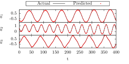
Figure 2: The principal component coefficients reconstructed from the pointwise data (red) for a new trajectory that was not used in the Koopman eigenfunction computation. The actual values are indicated by the black lines. There is good agreement between the predicted and true principal component values, and our approach accurately captures the approach of the trajectory to the limit cycle. We reiterate that each principal component value was reconstructed independently.

Using this pair of parameterizations, we reconstruct the PCA coefficients from pointwise data. Figure 2 demonstrates the quality of this reconstruction with data from a randomly initialized trajectory that approaches the limit cycle. In the figure, the black lines denote the true coefficient of each principal component, and the red dots indicate the predicted value. Note that this trajectory was not used to compute the Koopman eigenfunctions; furthermore, the fact that the data are a time series was not used in making this prediction, and each measurement of $\bm{\hat{x}}$ was considered individually.

Visually, the agreement between the predicted and actual states is good, but there are errors in the reconstruction. Over the time window $t\in[0,400]$, which is shown in Fig. 2, the relative error in each of the principal components is $e_{1}=0.0405$, $e_{2}=0.0655$, and $e_{3}=0.0496$, where $e_{i}=\|a_{i}^{\text{(true)}}-a_{i}^{\text{(pred)}}\|/\|a_{i}^{(\text{true})}\|$, where $\|\cdot\|=\left(\int_{0}^{400}(\cdot)^{2}\;dt\right)^{1/2}$. In general, the accuracy of this approach is better for points nearer to the limit cycle, and the relative errors over the window $t\in[0,4000]$, which (as shown in the supplement) contains points closer to the limit cycle, are only $e_{1}=0.0140$, $e_{2}=0.0295$, and $e_{3}=0.0234$ respectively.

In this example, we have not yet discussed the dimensionality of the data, but as stated previously, the number of measurements in each data set is critical for this approach to be justifiable mathematically. Our focus is on dynamics near the limit cycle, which in this problem are effectively two dimensional. However, the data lie on a two-dimensional nonlinear manifold that PCA, which fits the data with a hyperplane, requires three principal components to accurately represent. Therefore, the identified mapping is from $\mathbb{R}^{2}$ to a two-dimensional nonlinear manifold in $\mathbb{R}^{3}$, and not from $\mathbb{R}^{2}$ to $\mathbb{R}^{3}$.

Conclusions. We have presented a method for data fusion or state reconstruction that is suitable for nonlinear systems and exploits the existence of an intrinsic set of variables generated by the eigenfunctions of the Koopman operator. Rather than mapping directly between different sets of measurements, our method focuses on generating an independent mapping to and from the intrinsic variables for each heterogeneous set of measurements. In principle, this can be accomplished as long as a mapping from each set of measurements (or measurements and their time delays) to the system state exists, and the benefit of this approach is that the majority of the required data can be obtained independently, and only a single “joint” pair of data is needed. The keys to this method are: (i) the invariance of the Koopman eigenvalues to invertible transformations, (ii) the fact that the eigenfunctions parameterize state space, and (iii) the ability of data-driven methods, such as EDMD, to produce approximations of the eigenvalues and eigenfunctions that are “accurate enough” to allow these properties to be exploited in practical settings.

Acknowledgements The authors gratefully acknowledge support from the National Science Foundation (DMS-1204783) and the AFOSR.

Appendix A Supplementary Material

In this supplement, we present an expanded discussion of some key points in the data fusion procedure outlined in the manuscript. In particular, we focus on the ability of the Koopman eigenfunctions to parameterize state space, the accuracy of the mapping between eigenfunctions obtained with different sets of data, and the quality of the reconstruction for our illustrative example over a longer time horizon. Each of these points has been touched upon in the manuscript, and our objective is simply to present some additional supporting evidence rather than introduce any new concepts.

Measurement Parameterization and Mapping

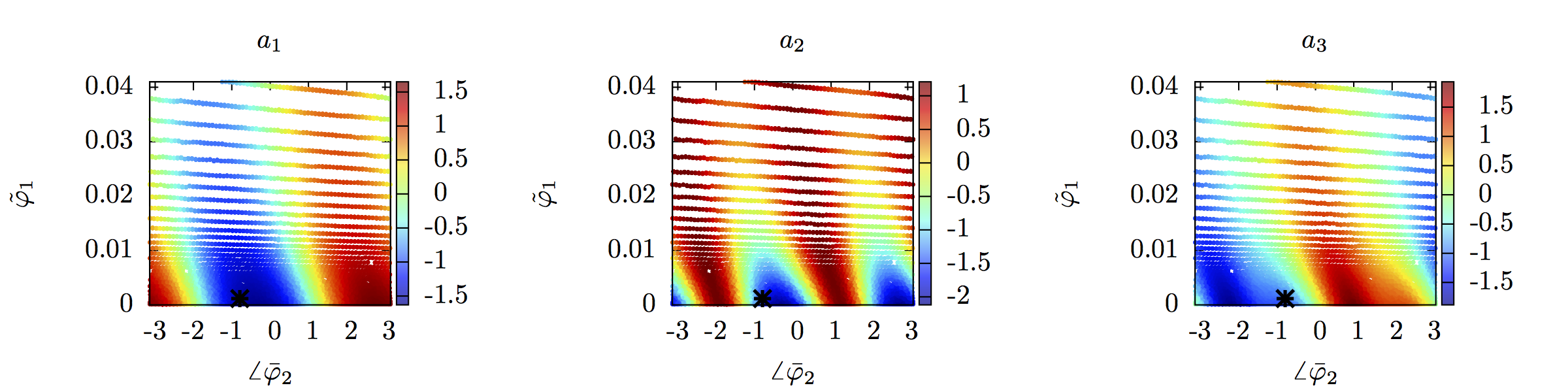
Figure 3: Pseudo-color plot of the first three principal component coefficients, $a_{1}$, $a_{2}$, and $a_{3}$, as a function of two of the Koopman eigenfunctions, $\tilde{\varphi}_{1}$ and $\angle\tilde{\varphi}_{2}$. Note that all three of these coefficients appear to be smooth functions of the Koopman eigenfunction values, and hence $\tilde{\varphi}_{1}$ and $\angle\tilde{\varphi}_{2}$ form an effective action-angle coordinate system for the nonlinear “slow manifold” in principal component space. The black $x$ denotes the point in the joint data set that was used for registration purposes.

In the manuscript, we claim that our set of two Koopman eigenfunctions parameterizes both the PCA data and the point-wise measurement data, and give a visual example of this in Fig. 1. However, the final step in reconstructing the principal component coefficients (or point-wise measurements) is mapping from the intrinsic coordinates defined by the Koopman eigenfunctions to the original set of variables. In principle, the Koopman modes would allow this to be done, and would effectively act as coefficients in a truncated series expansion of the inverse map. To simplify our code, we instead use interpolation methods appropriate for scattered data. These methods could include moving least squares interpolants, but we make use of the linear interpolation routine implemented by the griddata command in Scipy. This routine uses a Delaunay triangulation in conjunction with Barycentric interpolation to create a piecewise linear approximation of the inverse function. Figure 3 plots the coefficient of the $i$-th principal component as a function of the two Koopman eigenfunctions; note that the value of the principal component varies continuously and “slowly,” which is why the simple piecewise linear interpolant employed here is sufficient to produce a good approximation of the mapping from the Koopman eigenfunction values to the principal component coefficients. With far fewer data points or more complicated attractors, this mapping may be more difficult to satisfactorily approximate, and would require more sophisticated interpolation/extrapolation algorithms than what we used here.

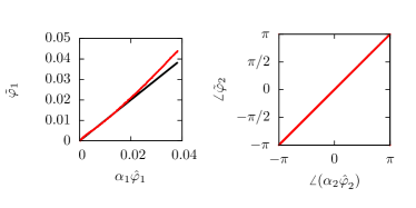
Figure 4: Plot of $\tilde{\varphi}_{1}$ as a function of $\alpha_{1}\hat{\varphi}_{1}$ and $\angle\tilde{\varphi}_{2}$ as a function of $\angle(\alpha_{2}\hat{\varphi}_{2})$. The data points are indicated by the red dots; the black line is a guide for the eye. Ideally, the $\alpha$ are chosen to make these quantities equal. While this is essentially the case for $\varphi_{2}$, the accuracy of the fit degrades as either $\tilde{\varphi}_{1}$ or $\hat{\varphi}_{1}$ become larger. For this problem, our approximation of this eigenfunction is reasonably accurate when $|\tilde{\varphi}_{1}|<0.03$, and tends to be higher for points nearer to the limit cycle (where $|\tilde{\varphi}_{1}|=0$). At larger values, the clear systemic error that appears in this plot will manifest itself as a systematic error in the reconstruction (or merging) of new data points.

A related issue involves the data used in the approximation. In Fig. 3, it is clear that the majority of the data lies near $\hat{\varphi}_{1}=0$. There are two reasons for this. First, it is easier to collect data near the limit cycle simply due to the dynamics of the underlying system. Furthermore, the magnitude of the eigenfunction, $\varphi_{1}$, typically grows rapidly as one gets further from the limit cycle, and will even have singularities at the unstable fixed point. However, because the EDMD procedure uses data to approximate the eigenfunctions, it is important to have data further away from the limit cycle despite the (possible extra) effort in obtaining them. It is for this reason that we use 20 independently initialized trajectories rather than a single, longer trajectory.

In the manuscript, we noted that the accuracy of our data fusion decreases the further we get from the limit cycle. Figure 4 quantifies this effect. The figure shows the amplitude and phase of what ought to be the same eigenfunction (approximated through different sets of heterogeneous observations) as functions of one another. Ideally, these two representations should coincide, and for $\angle\tilde{\varphi}_{2}$ and $\angle\hat{\varphi}_{2}$ they, in effect, do. However, this is not the case for $\tilde{\varphi}_{1}$ and $\hat{\varphi}_{1}$, which are shown in the left plot. In theory, both of these eigenfunctions are zero on the periodic orbit, and their absolute value increases for points that are further away. The figure, with the $\alpha$ we computed, shows good agreement between the value of the eigenfunctions when their absolute values are small, but a growing systematic error when they are large. This difference is one of the causes of the errors we observe, and why the accuracy of our approach decreases as one gets further from the limit cycle. There are, in general, open questions about the validity of EDMD computations performed on subsets of state space, and how they impact the accuracy of the numerically computed eigenfunctions. For this problem, the predictions our method produces are accurate (to the eye) when $|\hat{\varphi}_{1}|<0.03$, but beyond that point, the predicted and actual solutions will be quantitatively and visually different due to a combination of sparse data and the “partial domain” issue.

Measurement Reconstruction

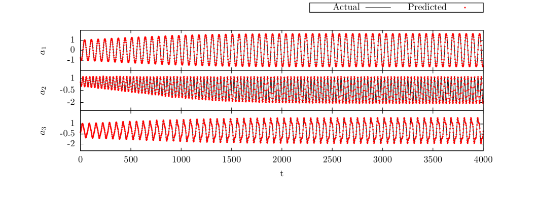
Figure 5: Plot of the predicted principal component coefficients obtained using the data merging procedure outlined in the paper. This figure is a “zoomed out” version of Fig. 2 and shows both the true and reconstructed values for $t\in[0,4000]$, which highlights that this approach accurately recovers both the periodic oscillations and the “envelope” that contains them.

In Fig. 2, we reconstructed the principal component values from point-wise data for a new, randomly-initialized trajectory on the interval $t\in[0,400]$ Figure 5 shows the reconstructed state using the same trajectory, but over the time interval $t\in[0,4000]$. Overall, there is good agreement between the predicted and actual principal component coefficients; in particular, our approach accurately recovers the “envelope” of the oscillation in all three principal components. Although not obvious to the eye, the relative error decreases from $\sim$5% in the short window to $\sim$2% over the longer time interval. Recall that neither time nor the fact that this data are a trajectory are used explicitly in the reconstruction; the increase in accuracy is solely due to the fact that points at later times are near to the limit cycle.

Figure 6: Three different views of the original principal component data (shown in red), the reconstructed principal component values of the 20 trajectories that comprise the point-wise data set used in the manuscript (shown in blue), and the reconstruction with 20 new point-wise trajectories that were not used in the Koopman computation (also shown in blue). Though there is some error, which can most easily be seen in the center plot, our approach effectively embeds these new points on the nonlinear, two-dimensional manifold that the original set of principal component coefficients is confined to. The region with the largest error occurs near the “hole” in the center of the manifold, and corresponds to points that are furthest from the limit cycle.

Finally, Fig. 6 shows the original set of PCA data in blue, and 40 trajectories consisting of the predicted values from the point-wise reconstruction, which are shown in red. Twenty of the trajectories were the data used to construct the point-wise approximation of the Koopman eigenfunctions, and twenty of the trajectories are “new”. The three plots in the figure show the same data from three different views. The point of this figure is to demonstrate that our predicted values lie on (or near) the nonlinear manifold on which the original PCA data live. There are clearly some errors, which become particularly pronounced using the view in the center plot, that appear as “noise” about an otherwise parabolic shape. As stated previously, these errors are most apparent near the “hole” in the center of the manifold, which corresponds to points far away from the limit cycle where our parameterizations are known to be inaccurate. However, even these errors are small compared to the total change in the coefficient of the second principal component. As a result, while this method is certainly not error free, it is able to effectively map point-wise measurements to principal component values (and vice versa) as long as the numerical approximations of the necessary Koopman eigenfunctions are “accurate enough” to serve as a set of intrinsic variables.

References

- Hall and Llinas (1997) D. L. Hall and J. Llinas, Proceedings of the IEEE 85, 6 (1997).
- Pohl and Van Genderen (1998) C. Pohl and J. Van Genderen, International Journal of Remote Sensing 19, 823 (1998).
- Yocky (1995) D. A. Yocky, JOSA A 12, 1834 (1995).
- Simon (2006) D. Simon, Optimal state estimation: Kalman, H infinity, and nonlinear approaches (John Wiley & Sons, 2006).
- Stengel (2012) R. F. Stengel, Optimal control and estimation (Courier Dover Publications, 2012).
- Bishop and Welch (2001) G. Bishop and G. Welch, Proc of SIGGRAPH, Course 8, 41 (2001).
- Adrian and Moin (1988) R. J. Adrian and P. Moin, Journal of Fluid Mechanics 190, 531 (1988).
- Adrian (1994) R. J. Adrian, Applied Scientific Research 53, 291 (1994).
- Guezennec (1989) Y. Guezennec, Physics of Fluids A: Fluid Dynamics (1989-1993) 1, 1054 (1989).
- Ho and Lee (1964) Y.-C. Ho and R. Lee, Automatic Control, IEEE Transactions on 9, 333 (1964).
- Bonnet et al. (1994) J. Bonnet, D. Cole, J. Delville, M. Glauser, and L. Ukeiley, Experiments in Fluids 17, 307 (1994).
- Druault et al. (2010) P. Druault, M. Yu, and P. Sagaut, International Jurnal for Numerical Methods in Fluids 62, 906 (2010).
- Murray and Ukeiley (2007) N. E. Murray and L. S. Ukeiley, Journal of Turbulence (2007).
- Naguib et al. (2001) A. Naguib, C. Wark, and O. Juckenhöfel, Physics of Fluids (1994-present) 13, 2611 (2001).
- Fieguth (2010) P. Fieguth, Statistical image processing and multidimensional modeling (Springer, 2010).
- Willcox (2006) K. Willcox, Computers & Fluids 35, 208 (2006).
- Dsilva et al. (2013) C. J. Dsilva, R. Talmon, N. Rabin, R. R. Coifman, and I. G. Kevrekidis, The Journal of Chemical Physics 139, 184109 (2013).
- Bright et al. (2013) I. Bright, G. Lin, and J. N. Kutz, Physics of Fluids (1994-present) 25, 127102 (2013).
- Koopman (1931) B. O. Koopman, Proceedings of the National Academy of Sciences of the United States of America 17, 315 (1931).
- Koopman and Neumann (1932) B. Koopman and J. v. Neumann, Proceedings of the National Academy of Sciences of the United States of America 18, 255 (1932).
- Mauroy et al. (2013) A. Mauroy, I. Mezić, and J. Moehlis, Physica D: Nonlinear Phenomena 261, 19 (2013).
- Mauroy and Mezić (2012) A. Mauroy and I. Mezić, Chaos: An Interdisciplinary Journal of Nonlinear Science 22, 033112 (2012).
- Budišić et al. (2012) M. Budišić, R. Mohr, and I. Mezić, Chaos: An Interdisciplinary Journal of Nonlinear Science 22, 047510 (2012).
- Lee and Verleysen (2007) J. A. Lee and M. Verleysen, Nonlinear dimensionality reduction (Springer, 2007).
- Chorin et al. (2000) A. J. Chorin, O. H. Hald, and R. Kupferman, Proceedings of the National Academy of Sciences 97, 2968 (2000).
- Chorin et al. (2002) A. J. Chorin, O. H. Hald, and R. Kupferman, Physica D: Nonlinear Phenomena 166, 239 (2002).
- Juang (1994) J.-N. Juang, Applied system identification (Prentice Hall, 1994).
- Mauroy and Mezic (2013) A. Mauroy and I. Mezic, in Decision and Control (CDC), 2013 IEEE 52nd Annual Conference on (2013) pp. 5234–5239.
- Mezić (2013) I. Mezić, Annual Review of Fluid Mechanics 45, 357 (2013).
- Rowley et al. (2009) C. W. Rowley, I. Mezić, S. Bagheri, P. Schlatter, and D. S. Henningson, Journal of Fluid Mechanics 641, 115 (2009).
- Williams et al. (2014) M. O. Williams, I. G. Kevrekidis, and C. W. Rowley, arXiv preprint arXiv:1408.4408 (2014).
- Schmid (2010) P. J. Schmid, Journal of Fluid Mechanics 656, 5 (2010).
- Schmid et al. (2011) P. Schmid, L. Li, M. Juniper, and O. Pust, Theoretical and Computational Fluid Dynamics 25, 249 (2011).
- Schmid et al. (2012) P. J. Schmid, D. Violato, and F. Scarano, Experiments in Fluids 52, 1567 (2012).
- Seena and Sung (2011) A. Seena and H. J. Sung, International Journal of Heat and Fluid Flow 32, 1098 (2011).
- Susuki and Mezic (2013) Y. Susuki and I. Mezic, IEEE Transactions on Power Systems (2013).
- Susuki and Mezić (2012) Y. Susuki and I. Mezić, Power Systems, IEEE Transactions on 27, 1182 (2012).
- Susuki and Mezić (2011) Y. Susuki and I. Mezić, IEEE Transactions on Power Systems 26, 1894 (2011).
- Nadler et al. (2005) B. Nadler, S. Lafon, R. Coifman, and I. Kevrekidis, in NIPS (2005).
- Lancaster and Salkauskas (1981) P. Lancaster and K. Salkauskas, Mathematics of Computation 37, 141 (1981).
- Levin (1998) D. Levin, Mathematics of Computation of the American Mathematical Society 67, 1517 (1998).
- Jones et al. (2001) E. Jones, T. Oliphant, and P. Peterson, http://www. scipy. org/ (2001).
- Holmes et al. (1998) P. Holmes, J. L. Lumley, and G. Berkooz, Turbulence, coherent structures, dynamical systems and symmetry (Cambridge university press, 1998).
- Li and Liu (2002) S. Li and W. K. Liu, Applied Mechanics Reviews 55, 1 (2002).
- Belytschko et al. (1994) T. Belytschko, Y. Y. Lu, and L. Gu, International Journal for Numerical Methods in Engineering 37, 229 (1994).
- Belytschko et al. (1996) T. Belytschko, Y. Krongauz, D. Organ, M. Fleming, and P. Krysl, Computer Methods in Applied Mechanics and Engineering 139, 3 (1996).
- Samet (1990) H. Samet, Applications of Spatial Data Structures: Computer Graphics, Image Processing, and GIS (Addison-Wesley Longman Publishing Co., Inc., Boston, MA, USA, 1990).
- Wendland (1999) H. Wendland, Mathematics of Computation of the American Mathematical Society 68, 1521 (1999).
- Fasshauer (1996) G. E. Fasshauer, in Proceedings of Chamonix, Vol. 1997 (Citeseer, 1996) pp. 1–8.
- Karniadakis and Sherwin (2013) G. Karniadakis and S. Sherwin, Spectral/hp element methods for computational fluid dynamics (Oxford University Press, 2013).
- Cockburn et al. (2000) B. Cockburn, G. E. Karniadakis, and C.-W. Shu, The development of discontinuous Galerkin methods (Springer, 2000).
- Trefethen (2000) L. N. Trefethen, Spectral methods in MATLAB, Vol. 10 (SIAM, 2000).
- Weideman and Reddy (2000) J. A. Weideman and S. C. Reddy, ACM Transactions on Mathematical Software (TOMS) 26, 465 (2000).