The Rise of Solitons in Sine-Gordon Field Theory: From Jacobi Amplitude to Gudermannian Function

Abstract

We show how the famous soliton solution of the classical sine-Gordon field theory in $(1+1)$-dimensions may be obtained as a particular case of a solution expressed in terms of the Jacobi amplitude, which is the inverse function of the incomplete elliptic integral of the first kind.

Keywords: Solitons, Sine-Gordon Field Theory, Elliptic Integrals, Jacobi Amplitude

I Introduction

The sine-Gordon field theory and the associated massive Thirring model coleman are some of the best studied quantum field theories. In view of its connections to other important physical models, some of which in principle admit actual realizations in nature kosterlitz ; samuel , a huge mass of important exact results have been obtained for this fascinating integrable system solitons ; MondainiJSP ; MondainiJPA ; MondainiJMP . However, no less fascinating are the remarkable mathematical and physical properties of its soliton (or “solitary wave”) solutions which have contributed, along the last decades, to turn the physics of solitons into a very active research topic.

In this work we present a simple and yet appealing step-by-step derivation of a more general solution for the classical sine-Gordon field theory in (1+1)-dimensions in terms of a special kind of elliptic function, namely the Jacobi amplitude, which has the famous sine-Gordon soliton solution as a particular case. Despite the fact that the connection between solitons and Jacobi elliptic functions has already been explored in cervero , we believe this work comes to shed more light on this interesting subject, helping to fill in a gap existing in the corresponding specialized literature.

II An alternative pathway to solitons in sine-Gordon field theory

II.1 The Jacobi amplitude function

We start by considering the following theory describing a real scalar field in (1+1)-dimensions ($\phi\equiv\phi(x,t)$),

$$\mathcal{L}=\frac{1}{2}\partial_{\mu}\phi\partial^{\mu}\phi-V(\phi),$$ (1)

where the potential term is given by

$$V(\phi)=2\alpha\cos(\beta\phi)+2\gamma.$$ (2)

The above Lagrangian gives rise, through the Euler-Lagrange equation, $\partial_{\mu}\left(\frac{\partial\mathcal{L}}{\partial(\partial_{\mu}\phi)}\right)=\frac{\partial\mathcal{L}}{\partial\phi}$, to the following field equation

$$\partial_{\mu}\partial^{\mu}\phi\equiv\Box\phi\equiv\left(\frac{1}{c^{2}}\frac{\partial^{2}}{\partial t^{2}}-\frac{\partial^{2}}{\partial x^{2}}\right)\phi=-\frac{\partial V(\phi)}{\partial\phi}.$$ (3)

Notice that since Equation (3) is invariant under Lorentz transformations ($x^{\mu}\rightarrow x^{\prime\mu}=\Lambda^{\mu}\,_{\nu}x^{\nu}$)rbef , its solutions may be obtained through the solutions of the corresponding equation for the static case ($\phi\equiv\phi(x)$) by a simple Lorentz boost, namely $x-x_{0}\rightarrow(x-x_{0}-vt)/\sqrt{1-(v^{2}/c^{2})}$, for arbitrary $v$ ($|v|<c\approx 3\times 10^{8}\,{\rm m/s}$)jackiw ; rajaraman . Thus, in what follows, we will focus on the solutions of the equation

$$\frac{d^{2}\phi}{dx^{2}}=\frac{dV}{d\phi}.$$ (4)

Indeed, by multiplying the above equation by $d\phi/dx$ we obtain

$$\frac{d\phi}{dx}\frac{d^{2}\phi}{dx^{2}}=\frac{d\phi}{dx}\frac{dV}{d\phi}\Rightarrow\frac{d}{dx}\left[\frac{1}{2}\left(\frac{d\phi}{dx}\right)^{2}\right]=\frac{dV}{dx},$$ (5)

which, after an integration with respect to $x$ and some algebra, may be rewritten as

$$dx^{\prime}=\pm\frac{d\phi^{\prime}}{\sqrt{2V(\phi^{\prime})}}.$$ (6)

By integrating both sides of the above equation, from $x^{\prime}=x_{0}$ to $x^{\prime}=x$ ($\phi^{\prime}=\phi(x_{0})$ to $\phi^{\prime}=\phi(x)$), we get

$$x-x_{0}=\pm\int_{\phi(x_{0})}^{\phi(x)}\frac{d\phi^{\prime}}{\sqrt{2V(\phi^{\prime})}}.$$ (7)

In order to compute the above integral, we must firstly notice that the potential, shown in Equation (2), may be rewritten as

$$V(\phi^{\prime})=2(\alpha+\gamma)\left[1-\frac{2\alpha}{\alpha+\gamma}\sin^{2}\left(\frac{\beta\phi^{\prime}}{2}\right)\right].$$ (8)

Thus, by making the change of variables $\phi^{\prime}\rightarrow\theta^{\prime}=\frac{\beta}{2}\phi^{\prime}$, defining $k^{2}=\frac{2\alpha}{\alpha+\gamma}$ and choosing $x_{0}$ such that $\phi(x_{0})=0\Rightarrow\theta_{0}=0$, we are left with

$$x-x_{0}=\pm\frac{k}{\beta\sqrt{2\alpha}}\int_{0}^{\theta}\frac{d\theta^{\prime}}{\sqrt{1-k^{2}\sin^{2}{\theta^{\prime}}}}.$$ (9)

The integral appearing in Equation (9) is called an incomplete elliptic integral of the first kind, $F(\theta,k)$, whereas $k$ is called the elliptic modulus or eccentricity. The upper limit, $\theta$, of this integral may be written in terms of the Jacobi amplitude (the inverse function of the incomplete elliptic integral of the first kind) as grad ; jacobi .

$$\theta=\pm\,F^{-1}\left(\frac{\beta\sqrt{2\alpha}}{k}(x-x_{0}),k\right)\equiv\pm\,{\rm am}\left(\frac{\beta\sqrt{2\alpha}}{k}(x-x_{0}),k\right).$$ (10)

Notice that, from the above definition, we have $F({\rm am}\left(x,k\right),k)=x$.

The solution of Equation (4) may be, finally, written as

$$\phi(x)=\pm\frac{2}{\beta}\,{\rm am}\left(\frac{\beta\sqrt{2\alpha}}{k}(x-x_{0}),k\right).$$ (11)

Hence, from the above equation, we may notice that

$$\phi(x_{0})=\pm\frac{2}{\beta}\,{\rm am}\left(0,k\right)=0,$$ (12)

as it should.

II.2 The case $k=1$: The Gudermannian function and the soliton solution of sine-Gordon equation

From the definition $k^{2}=2\alpha/(\alpha+\gamma)$ we may obviously see that when $\gamma=\alpha$ we have $k=1$. Hence, the solution for Equation (4) with the potential given by

$$V(\phi)=2\alpha[1+\cos(\beta\phi)],$$ (13)

may be obtained as a special case of the solution presented in Equation (11). Indeed, since ${\rm am}(x,1)={\rm gd}\,x\equiv 2\arctan(e^{x})-\pi/2$, where ${\rm gd}\,x$ is called the Gudermannian function (a special function which relates the circular functions to the hyperbolic ones without using complex numbers, named after Christoph Gudermann (1798 - 1852)), we are left with

$$\phi(x)=\pm\frac{2}{\beta}\,{\rm am}\left(\beta\sqrt{2\alpha}(x-x_{0}),1\right) = \pm\frac{2}{\beta}\,{\rm gd}\left(\beta\sqrt{2\alpha}(x-x_{0})\right)$$ (14)

$$\equiv \pm\frac{4}{\beta}\arctan\left[\exp\left(\beta\sqrt{2\alpha}(x-x_{0})\right)\right]\mp\frac{\pi}{\beta}.$$

Last but not least, we must notice that by substituting the Equation (14) into Equation (3) and making the change (Lorentz boost) $x-x_{0}\rightarrow(x-x_{0}-vt)/\sqrt{1-(v^{2}/c^{2})}$, we obtain the famous sine-Gordon field equation, namely

$$\Box\phi_{S}+2\alpha\beta\sin\beta\phi_{S}=0,$$ (15)

where $\phi_{S}\equiv\phi_{S}(x,t)$ is the no less famous soliton/anti-soliton solution jackiw ; rajaraman , given by

$$\phi_{S}(x,t)=\pm\frac{4}{\beta}\arctan\left[\exp\left(\beta\sqrt{2\alpha}\frac{x-x_{0}-vt}{\sqrt{1-(v^{2}/c^{2})}}\right)\right].$$ (16)

This result allows us to characterize the Lorentz boosted, and shifted by $\pi/\beta$, version of the solution in terms of the Jacobi amplitude shown in Equation (11), namely

$$\phi(x,t)=\pm\frac{2}{\beta}\,{\rm am}\left(\frac{\beta\sqrt{2\alpha}}{k}\frac{x-x_{0}-vt}{\sqrt{1-(v^{2}/c^{2})}},k\right)\pm\frac{\pi}{\beta},$$ (17)

as a generalization of the sine-Gordon soliton/anti-soliton solution for $k\neq 1$.

III Concluding remarks

We would like to make a few comments about the soliton solution, shown in Equation (16), and its generalized version, shown in Equation (17). Firstly, we may notice by comparing the Figures 1 and 2 how different are these solutions, where we would like to highlight the doubly periodic behaviour of the Jacobi amplitude solution.

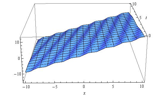
Figure 1: The Jacobi amplitude solution given by Equation (17) with $\alpha=0.50$, $\beta=2.00$, $x_{0}=0$, $k=0.99$ and $v=0.50c$

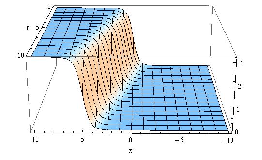
Figure 2: The soliton solution given by Equation (16) with $\alpha=0.50$, $\beta=2.00$, $x_{0}=0$, $k=1.00$ and $v=0.50c$

Finally, let us observe that, as remarked in jackiw , this soliton solution, though arising in a classical field theory, looks very much like a classical particle since its energy density is localized at a point ($x=x_{0}$) and its total energy for a static field configuration ($\phi_{S}\equiv\phi_{S}(x)$), namely

$$E(\phi_{S})=\int_{-\infty}^{\infty}dx\left[\frac{1}{2}\left(\frac{d\phi}{dx}\right)^{2}+V(\phi)\right]=\frac{8\sqrt{2\alpha}}{\beta},$$ (18)

is finite, just as we should expect.

References

- (1) Coleman, S. (1975) Quantum Sine-Gordon Equation as the Massive Thirring Model. Phys. Rev. D, 11, 2088-2097. http://dx.doi.org/10.1103/PhysRevD.11.2088
- (2) Kosterlitz, J.M. (1974) The Critical Properties of the Two-Dimensional XY Model. J. Phys. C: Solid State Phys., 7, 1046-1060. http://dx.doi.org/10.1088/0022-3719/7/6/005
- (3) Samuel, S. (1978) Grand Partition Function in Field Theory with Applications to Sine-Gordon Field Theory. Phys. Rev. D, 18, 1916-1932. http://dx.doi.org/10.1103/PhysRevD.18.1916
- (4) Dauxois, T. and Peyrard, M. (2006) Physics of Solitons. Cambridge University Press, New York.
- (5) Mondaini, L. and Marino, E.C. (2005) Sine-Gordon/Coulomb Gas Soliton Correlation Functions and an Exact Evaluation of the Kosterlitz-Thouless Critical Exponent. J. Stat. Phys., 118, 767-779. http://dx.doi.org/10.1007/s10955-004-8828-y
- (6) Mondaini, L., Marino, E.C. and Schmidt, A.A. (2009) Vanishing Conductivity of Quantum Solitons in Polyacetylene. J. Phys. A: Math. Theor., 42, 055401. http://dx.doi.org/10.1088/1751-8113/42/5/055401
- (7) Mondaini, L. (2012) Thermal Soliton Correlation Functions in Theories with a Symmetry. J. Mod. Phys., 3, 1776-1780. http://dx.doi.org/10.4236/jmp.2012.311221
- (8) Cervero, J.M. (1986) Unveiling the Solitons Mistery: The Jacobi Elliptic Functions. Am. J. Phys., 54, 35-38. http://dx.doi.org/10.1119/1.14767
- (9) Mondaini, L. (2012) Obtaining a Closed-form Representation for the Dual Bosonic Thermal Green Function by Using Methods of Integration on the Complex Plane. Rev. Bras. Ens. Fis., 34, 3305. http://dx.doi.org/10.1590/S1806-11172012000300005
- (10) Jackiw, R. (1977) Quantum Meaning of Classical Field Theory. Rev. Mod. Phys., 49, 681-706. http://dx.doi.org/10.1103/RevModPhys.49.681
- (11) Rajaraman, R. (1987) Solitons and Instantons: An Introduction to Solitons and Instantons in Quantum Field Theory. Elsevier, Amsterdam.
- (12) Gradshteyn, I.S. and Ryzhik, I.M. (2000) Table of Integrals, Series, and Products. Academic Press, San Diego.
- (13) Weisstein, E.W. Jacobi Amplitude. MathWorld – A Wolfram Web Resource. http://mathworld.wolfram.com/JacobiAmplitude.html