Topological formula of the loop expansion of the colored Jones polynomials

Abstract.

We give a topological formula of the loop expansion of the colored Jones polynomials by using identification of generic quantum $\mathfrak{sl}_{2}$ representation with homological representations. This gives a direct topological proof of the Melvin-Morton-Rozansky conjecture, and a connection between entropy of braids and quantum representations.

1. Introduction

For $\alpha\in\{2,3,4,\ldots\}$ and an oriented knot $K$ in $S^{3}$, let $J_{K,\alpha}(q)\in\mathbb{Z}[q,q^{-1}]$ be the $\alpha$-colored Jones polynomial of $K$ normalized so that $J_{\textsf{Unknot},\alpha}(q)=1$. As Melvin-Morton proved [MeMo], by putting $q=e^{\hbar}$, the colored Jones polynomials can be expanded as a power series of two independent variables $\hbar\alpha$ and $\hbar$, as

$$J_{K,\alpha}(e^{\hbar})=\sum_{i=0}^{\infty}D^{(i)}(\hbar\alpha)\hbar^{i}=\sum_{i=0}^{\infty}\left(\sum_{k=0}^{\infty}d^{(i)}_{k}(\hbar\alpha)^{k}\right)\hbar^{i}.$$

Further, we put $z=e^{\hbar\alpha}$ and write the colored Jones polynomials as a function on $\hbar$ and $z$,

$$CJ_{K}(z,\hbar)=J_{K,\alpha}(e^{\hbar})=\sum_{i=0}^{\infty}V_{K}^{(i)}(z)\hbar^{i}.$$

We call $CJ_{K}$ the colored Jones function or, the loop expansion of quantum $\mathfrak{sl}_{2}$-invariant since it coincides with the $\mathfrak{sl}_{2}$ weight system reduction of the loop expansion of the Kontsevich invariant. In particular, the $i$-th coefficient $V^{(i)}(z)$ corresponds to the $(i+1)$-st loop part of the loop expansion of the Kontsevich invariant [Oh1].

Let $\nabla_{K}(z)$ be the Conway polynomial of $K$, characterized by the skein relation

$$\nabla_{\begin{minipage}{7.00043pt} \begin{picture}(10.0,10.0)\put(0.0,0.0){\vector(1,1){10.0}} \qbezier(10.0,0.0)(10.0,0.0)(7.0,3.0)\qbezier(3.0,7.0)(0.0,10.0)(0.0,10.0)\put(0.0,10.0){\vector(-1,1){0.0}} \end{picture} \end{minipage}}(z)-\nabla_{\begin{minipage}{7.00043pt} \begin{picture}(10.0,10.0)\put(10.0,0.0){\vector(-1,1){10.0}} \qbezier(0.0,0.0)(0.0,0.0)(3.0,3.0)\qbezier(7.0,7.0)(10.0,10.0)(10.0,10.0)\put(10.0,10.0){\vector(1,1){0.0}} \end{picture} \end{minipage}}(z)=z\nabla_{\begin{minipage}{7.00043pt} \begin{picture}(10.0,10.0)\put(0.0,10.0){\vector(-1,1){0.0}} \qbezier(0.0,0.0)(5.0,5.0)(0.0,10.0)\qbezier(10.0,0.0)(5.0,5.0)(10.0,10.0)\put(10.0,10.0){\vector(1,1){0.0}} \end{picture} \end{minipage}}(z),\ \ \ \nabla_{\sf Unknot}(z)=1$$

and let $\Delta_{K}(z)=\nabla_{K}(z^{\frac{1}{2}}-z^{-\frac{1}{2}})$ be the Alexander-Conway polynomial. The Alexander-Conway polynomial appears as one of the basic building block of $CJ_{K}$. The Melvin-Morton-Ronzansky conjecture [MeMo] (MMR conjecture, in short), proven in [BG], states that the $V^{(0)}(z)$ is equal to $\Delta_{K}(z)^{-1}$. More generally, $V^{(i)}(z)$ is a rational function whose denominator is $\Delta_{K}(z)^{2i+1}$ [Ro1].

In a theory of quantum invariants, the appearance of the Alexander-Conway polynomial is well-understood. The aforementioned rationality of $V^{(i)}(z)$ follows from Ronzansky’s rationality conjecture [Ro2] of the loop expansion of Kontsevich invariant, proven in [Kri]: The Aarhus integral computation of Kontsevich (or, LMO) invariant, based on a surgery presentation of knots, provides the desired rationality (see [GK, Section 1.2] for a brief summary of Kricker’s argument).

The clasper surgery [Ha] explains a geometric connection between the loop expansion and infinite cyclic covering [GR]. A null-clasper, a clasper with null-homologous leaves in the knot complement, lifts to a clasper in the infinite cyclic covering, and the loop expansion nicely behaves under the clasper surgery along null-claspers. Thus schematically speaking, the loop expansion provides a $\mathbb{Z}$-equivariant quantum invariants [GR] (for example, the 2-loop part can be interpreted as the $\mathbb{Z}$-equivariant Casson invariant, as discussed in [Oh2]), so it is not surprising that the Alexander-Conway polynomial appears in the loop expansion.

Nevertheless, it is still mysterious why the Alexander polynomial appears in such a particular and direct form. Even for the MMR conjecture, the simplest and the most fundamental rationality result, the situation is not so good as we want. In a known proof, one uses quantum-invariant-like treatment of the Alexander-Conway polynomial such as, state-sum, R-matrix, or weight systems so its topological content is often indirect.

In this paper, we give a topological formula of $CJ_{K}$ by using homological braid group representations (Theorem 3.1). Our starting point is a recent result in [I, Koh] that identifies certain homological representations introduced by Lawrence [La] with generic $U_{q}(\mathfrak{sl}_{2})$ representations. This allows us to translate a construction of the colored Jones function in terms of corresponding homological representations. Also, in Section 4 we discuss a connection among the entropy of braids, quantum representations, and the growth of quantum $\mathfrak{sl}_{2}$ invariants inspired from topological point of view.

One may notice that our approach is similar to Lawrence-Bigelow’s approach of Jones polynomial [Big2, La2], but there are several critical differences: We give a formula of the loop expansion $CJ_{K}$ but do not provide a formula of each individual colored Jones polynomials. Our formula uses closed braid representatives, whereas Lawrence-Bigelow description uses plat representatives and intersection products.

It should be emphasized that quantum representations coming from finite dimensional $U_{q}(\mathfrak{sl}_{2})$-module is not identified with homological representation. This is the reason why we do not have a direct topological formula of usual colored Jones polynomials.

Our topological description leads to several insights. First, the MMR conjecture is now obtained as a direct consequence of our topological formula. By putting $\hbar=0$, topological considerations show that the homological representations is equal to the symmetric powers of the reduced Burau representation, so they naturally lead to the Alexander-Conway polynomial. Second, our formula gives a new and direct way to calculate $CJ_{K}(z,\hbar)$ without knowing or computing individual colored Jones polynomial $J_{K,\alpha}(q)$ or appealing surgery presentation of knots, although a general calculation is still difficult.

2. A topological description of generic quantum $\mathfrak{sl}_{2}$ representation

In this section we review the result in [I] that identifies a generic quantum $\mathfrak{sl}_{2}$ representation given in [JK] with Lawrence’s homological representation and some additional arguments to treat non-generic case.

Throughout the paper, we use the following notations and conventions. The $q$-numbers, $q$-factorials, and $q$-binomial coefficients are defined by

$$[n]_{q}=\frac{q^{\frac{n}{2}}-q^{-\frac{n}{2}}}{q^{\frac{1}{2}}-q^{-\frac{1}{2}}},\ \ [n]_{q}!=[n]_{q}[n-1]_{q}\cdots[2]_{q}[1]_{q},\ \ \left[\!\!\begin{array}[]{c}n\\ j\end{array}\!\!\right]_{q}=\frac{[n]_{q}!}{[n-j]_{q}![j]_{q}!},$$

respectively. This convention is different from one in [I, JK]. The quantum parameter $q$ in this paper corresponds to $q^{2}$ in [I, JK]. We always assume that the braid group $B_{n}$ is acting from left.

Let $R$ be a commutative ring. For $R$-modules (resp. $RB_{n}$-modules) $V$ and $W$, we denote $V\cong_{\mathcal{Q}}W$ if they are isomorphic over the quotient field $\mathcal{Q}$ of $R$. Namely, $C\cong_{\mathcal{Q}}W$ implies $V\otimes_{R}\mathcal{Q}$ and $W\otimes_{R}\mathcal{Q}$ are isomorphic as $\mathcal{Q}$-modules (resp. $\mathcal{Q}B_{n}$-module).

For a subring $R\subset\mathbb{C}$, let $R[x^{\pm 1}]$ be the Laurent polynomial ring, and for an $R[x^{\pm 1}]$-module $V$ and $c\in\mathbb{C}$, we denote the specialization of the variable $x$ to complex parameter $c$ by $V|_{x=c}$.

2.1. Generic quantum representation

Let $\mathbb{C}[[\hbar]]$ be the algebra of the complex formal power series in one variable $\hbar$, and we put $q=e^{\hbar}$, as usual. A quantum enveloping algebra $U_{\hbar}(\mathfrak{sl}_{2})$ is a topological Hopf algebra over $\mathbb{C}[[\hbar]]$ generated by $H,E,F$ subjected to the relations

$$\begin{cases}[H,E]=2E,\;\;\;[H,F]=-2F,\\ {}\displaystyle[E,F]=\frac{\sinh(\frac{\hbar H}{2})}{\sinh(\frac{\hbar}{2})}=\frac{e^{\frac{\hbar H}{2}}-e^{-\frac{\hbar H}{2}}}{e^{\frac{\hbar}{2}}-e^{-\frac{\hbar}{2}}}\end{cases}$$

$U_{\hbar}(\mathfrak{sl}_{2})$ is a quasi-triangular topological Hopf algebra and a universal $R$-matrix $\mathcal{R}\in U_{\hbar}(\mathfrak{sl}_{2})\otimes U_{\hbar}(\mathfrak{sl}_{2})$ is given by

(2.1) $$\mathcal{R}=e^{\frac{\hbar}{4}(H\otimes H)}\left(\sum_{n=0}^{\infty}q^{\frac{n(n-1)}{4}}\frac{(q^{\frac{1}{2}}-q^{-\frac{1}{2}})^{n}}{[n]_{q}!}E^{n}\otimes F^{n}\right).$$

(Strictly speaking, here we need to use the topological tensor product $\widetilde{\otimes}$, the $\hbar$-adic completion of $U_{\hbar}(\mathfrak{sl}_{2})\otimes U_{\hbar}(\mathfrak{sl}_{2})$. To make notation simple, in the rest of the paper $\otimes$ should be regarded as the topological tensor product, if we should do so.)

For $\lambda\in\mathbb{C}^{*}$, let $V_{\lambda}$ be the Verma module of highest weight $\lambda$, a topologically free $U_{\hbar}(\mathfrak{sl}_{2})$-module generated by a highest weight vector $v_{0}$ with $Hv_{0}=\lambda v_{0}$ and $Ev_{0}=0$.

Now let us regard $\lambda$ as an abstract variable. Let $\widehat{V_{\hbar,\lambda}}$ be a $\mathbb{C}[\lambda][[\hbar]]$-module freely generated by $\{\widehat{v_{0}},\widehat{v_{1}},\ldots,\}$, equipped with an $U_{\hbar}(\mathfrak{sl}_{2})$-module structure

(2.2) $$\begin{cases}H\widehat{v}_{i}=(\lambda-2i)\widehat{v_{i}}\\ E\widehat{v}_{i}=\widehat{v}_{i-1}\\ F\widehat{v}_{i}=[i+1]_{q}[\lambda-i]_{q}\widehat{v}_{i+1}.\end{cases}$$

Here we put

$$[\lambda-i]_{q}=\frac{\sinh(\frac{1}{2}\hbar(\lambda-i))}{\sinh(\frac{1}{2}\hbar)}=\frac{e^{\frac{1}{2}\hbar(\lambda-i)}-e^{-\frac{1}{2}\hbar(\lambda-i)}}{e^{\frac{1}{2}\hbar}-e^{-\frac{1}{2}\hbar}}.$$

We call $\widehat{V_{\hbar,\lambda}}$ a generic Verma module.

For $j=0,1,\ldots,$ define

$$v_{j}=[\lambda]_{q}[\lambda-1]_{q}\cdots[\lambda-j+1]_{q}\widehat{v_{j}}$$

and let $V_{\hbar,\lambda}$ be the sub $U_{\hbar}(\mathfrak{sl}_{2})$-module of $\widehat{V_{\hbar,\lambda}}$ spanned by $\{v_{0},v_{1},\ldots\}$, with the action of $U_{\hbar}(\mathfrak{sl}_{2})$ given by

(2.3) $$\begin{cases}Hv_{i}=(\lambda-2i)v_{i}\\ Ev_{i}=[\lambda+1-i]_{q}v_{i-1}\\ Fv_{i}=[i+1]_{q}v_{i+1}.\end{cases}$$

For $c\not\in\mathbb{C}^{*}-\{1,2,\ldots\}$, $\widehat{V_{\hbar,\lambda}}|_{\lambda=c}$ is isomorphic to $V_{\hbar,\lambda}|_{\lambda=c}$ because $[\lambda]_{q}[\lambda-1]_{q}\cdots[\lambda-j+1]_{q}$ is invertible for all $j$. On the other hand, for $c\in\{1,2,\ldots,\}$, $v_{j}=0$ if $j>c$ and (2.3) shows that $V_{\hbar,\lambda}|_{\lambda=c}$ is nothing but the standard irreducible $U_{\hbar}(\mathfrak{sl}_{2})$-module of dimension $(c+1)$ whereas $\widehat{V_{\hbar,\lambda}}|_{\lambda=c}$ is infinite dimensional representation.

Let us define $\mathsf{R}:\widehat{V_{\hbar,\lambda}}\otimes\widehat{V_{\hbar,\lambda}}\rightarrow\widehat{V_{\hbar,\lambda}}\otimes\widehat{V_{\hbar,\lambda}}$ by $\mathsf{R}=e^{-\frac{1}{4}\hbar\lambda^{2}}T\mathcal{R}$, where $T:\widehat{V_{\hbar,\lambda}}\otimes\widehat{V_{\hbar,\lambda}}\rightarrow\widehat{V_{\hbar,\lambda}}\otimes\widehat{V_{\hbar,\lambda}}$ is the transposition map $T(v\otimes w)=w\otimes v$, and $\mathcal{R}$ is the universal $R$-matrix (2.1).

By putting $z=q^{\lambda-1}=e^{\hbar(\lambda-1)}$, the action of $\mathsf{R}$ is given by the formula

(2.4) $$\begin{cases}\mathsf{R}(\widehat{v}_{i}\otimes\widehat{v}_{j})=z^{-\frac{i+j}{2}}q^{-\frac{i+j}{2}}\sum_{n=0}^{i}q^{(i-n)(j+n)}q^{\frac{n(n-1)}{4}}\frac{[n+j]_{q}!}{[n]_{q}![j]_{q}!}\prod_{k=0}^{n-1}(z^{\frac{1}{2}}q^{-\frac{1+k+j}{2}}-z^{-\frac{1}{2}}q^{\frac{1+k+j}{2}})\widehat{v}_{j+n}\otimes\widehat{v}_{i-n}.\\ \mathsf{R}(v_{i}\otimes v_{j})=z^{-\frac{i+j}{2}}q^{-\frac{i+j}{2}}\sum_{n=0}^{i}q^{(i-n)(j+n)}q^{\frac{n(n-1)}{4}}\frac{[n+j]_{q}!}{[n]_{q}![j]_{q}!}\prod_{k=0}^{n-1}(z^{\frac{1}{2}}q^{\frac{1-i+k}{2}}-z^{-\frac{1}{2}}q^{-\frac{1-i+k}{2}})v_{j+n}\otimes v_{i-n}\end{cases}$$

Let $\mathbb{L}=\mathbb{Z}[q^{\pm 1},z^{\pm 1}]=\mathbb{Z}[e^{\pm\hbar},e^{\pm\hbar(\lambda-1)}]\subset\mathbb{C}[\lambda][[\hbar]]$ and let $V_{\mathbb{L}}$ and $\widehat{V_{\mathbb{L}}}$ be the sub free $\mathbb{L}$-module of $\widehat{V_{\hbar,\lambda}}$ and $V_{\hbar,\lambda}$, spanned by $\{\widehat{v_{0}},\ldots\}$ and $\{v_{0},\ldots\}$, respectively.

Since all the coefficients of the action of $\mathsf{R}$ (2.4) lie in $\mathbb{L}$, $\widehat{V_{\mathbb{L}}}$ and $V_{\mathbb{L}}$ are equipped with an $\mathbb{L}B_{n}$-module structure. We denote the corresponding braid group representations by

$$\widehat{\varphi_{\mathbb{L}}}:B_{n}\rightarrow\textrm{GL}(\widehat{V_{\mathbb{L}}}{}^{\otimes n}),\ \ \ \varphi_{\mathbb{L}}:B_{n}\rightarrow\textrm{GL}(V_{\mathbb{L}}^{\otimes n}).$$

These are decomposed as finite dimensional representations as follows. For $m\geq 0$, define $\widehat{V_{n,m}}\subset\widehat{V_{\mathbb{L}}}^{\otimes n}$ and $V_{n,m}\subset V_{\mathbb{L}}^{\otimes n}$ by

$$\begin{cases}\widehat{V_{n,m}}=\textrm{ker}\;(q^{H}-q^{\frac{n\lambda-2m}{2}})=\textrm{span}\{\widehat{v}_{i_{1}}\otimes\cdots\otimes\widehat{v}_{i_{n}}\>|\>i_{1}+\cdots+i_{n}=m\}.\\ V_{n,m}=\textrm{ker}\;(q^{H}-q^{\frac{n\lambda-2m}{2}})=\textrm{span}\{v_{i_{1}}\otimes\cdots\otimes v_{i_{n}}\>|\>i_{1}+\cdots+i_{n}=m\}\end{cases}$$

By (2.4), the $B_{n}$-action preserves both $\widehat{V_{n,m}}$ and $V_{n,m}$ so we have linear representations

$$\widehat{\varphi^{V}_{n,m}}:B_{n}\rightarrow\textrm{GL}(\widehat{V_{n,m}})\ \textrm{ and }\varphi^{V}_{n,m}:B_{n}\rightarrow\textrm{GL}(V_{n,m}).$$

We call the $\mathbb{L}B_{n}$-module $\widehat{V_{n,m}}$ the (generic) weight space of weight $q^{\frac{n\lambda-2m}{2}}$.

By definition, as $\mathbb{L}B_{n}$-modules, $\widehat{V_{\mathbb{L}}}^{\otimes n}$ and $V_{\mathbb{L}}^{\otimes n}$ split as

(2.5) $$\begin{cases}\widehat{V_{\mathbb{L}}}^{\otimes n}\cong\bigoplus_{m=0}^{\infty}\widehat{V_{n,m}}\\ V_{\mathbb{L}}^{\otimes n}\cong\bigoplus_{m=0}^{\infty}V_{n,m}\end{cases}$$

Finally, we define the space of (generic) null vectors $\widehat{W_{n,m}}$ by

$$\widehat{W_{n,m}}=\textrm{Ker}\,(E)\cap\widehat{V_{n,m}}.$$

Since the action of $B_{n}$ commutes with the action of $U_{q}(\mathfrak{sl}_{2})$, we have linear representation

$$\widehat{\varphi^{W}_{n,m}}:B_{n}\rightarrow\textrm{GL}(\widehat{W_{n,m}}).$$

In [JK, Lemma 13], it is shown that for $k=1,\ldots,m$, the map $F^{m-k}:\widehat{W_{n,k}}\rightarrow\widehat{V_{n,m}}$ is injection and that over the quotient field, $\widehat{V_{n,m}}$ splits as

(2.6) $$\widehat{V_{n,m}}\cong_{\mathcal{Q}}\bigoplus_{k=0}^{m}F^{m-k}\widehat{W_{n,k}}\cong_{\mathcal{Q}}\bigoplus_{k=0}^{m}\widehat{W_{n,k}},$$

hence combining with (2.5), we conclude that the $\mathbb{L}B_{n}$-module $\widehat{V_{\mathbb{L}}}^{\otimes n}$ splits, over the quotient field,

(2.7) $$\widehat{V_{\mathbb{L}}}^{\otimes n}\cong_{\mathcal{Q}}\bigoplus_{m=0}^{\infty}\bigoplus_{k=0}^{m}\widehat{W_{n,k}}.$$

2.2. Lawrence’s homological representations

Here we briefly review the definition of (geometric) Lawrence’s representation $L_{n,m}$. An explicit matrix of $L_{n,m}(\sigma_{i})$ and some details will be given in Appendix.

For $i=1,2,\ldots,n$, let $p_{i}=i\in\mathbb{C}$ and $D_{n}=\{z\in\mathbb{C}\>|\>|z|\leq n+1\}-\{p_{1},\ldots,p_{n}\}$ be the $n$-punctured disc. We identify the braid group $B_{n}$ with the mapping class group of $D_{n}$ so that the standard generator $\sigma_{i}$ corresponds to the right-handed half Dehn twist that interchanges the $i$-th and $(i+1)$-st punctures.

For $m>0$, let $C_{n,m}$ be the unordered configuration space of $m$-points in $D_{n}$,

$$C_{n,m}=\{(z_{1},\ldots,z_{m})\in D_{n}\>|\>z_{i}\neq z_{j}\;(i\neq j)\}/S_{m}$$

where $S_{m}$ is the symmetric group acting as permutations of the indices. For $i=1,\ldots,n$, let $d_{i}=(n+1)e^{(\frac{3}{2}+i\varepsilon)\pi\sqrt{-1}}\in\partial D_{n}$ where $\varepsilon>0$ is sufficiently small number, and we take $\mathbf{d}=\{d_{1},\ldots,d_{m}\}$ as a base point of $C_{n,m}$.

The first homology group $H_{1}(C_{n,m};\mathbb{Z})$ is isomorphic to $\mathbb{Z}^{\oplus n}\oplus\mathbb{Z}$, where the first $n$ components correspond to the meridians of the hyperplanes $\{z_{1}=p_{i}\}$ $(i=1,\ldots,n)$ and the last component corresponds to the meridian of the discriminant $\bigcup_{1\leq i<j\leq n}\{z_{i}=z_{j}\}$.

Let $\alpha:\pi_{1}(C_{n,m})\rightarrow\mathbb{Z}^{2}=\langle x,d\rangle$ be the homomorphism obtained by composing the Hurewicz homomorphism $\pi_{1}(C_{n,m})\rightarrow H_{1}(C_{n,m};\mathbb{Z})$ and the projection

$$H_{1}(C_{n,m};\mathbb{Z})=\mathbb{Z}^{\oplus n}\oplus\mathbb{Z}=\langle x_{1},\ldots,x_{n}\rangle\oplus\langle d\rangle\rightarrow\langle x_{1}+\cdots+x_{n}\rangle\oplus\langle d\rangle=\langle x\rangle\oplus\langle d\rangle=\mathbb{Z}\oplus\mathbb{Z}.$$

Let $\pi:\widetilde{C}_{n,m}\rightarrow C_{n,m}$ be the covering corresponding to $\textrm{Ker}\,\alpha$. We fix a lift $\widetilde{\mathbf{d}}\in\pi^{-1}(\mathbf{d})\subset\widetilde{C}_{n,m}$ and use $\widetilde{\mathbf{d}}$ as a base point of $\widetilde{C}_{n,m}$. By identifying $x$ and $d$ as deck translations, $H_{m}(\widetilde{C}_{n,m};\mathbb{Z})$ has a structure of $\mathbb{Z}[x^{\pm 1},d^{\pm 1}]$-module. Actually, it is known that $H_{m}(\widetilde{C}_{n,m};\mathbb{Z})$ is a free $\mathbb{Z}[x^{\pm 1},d^{\pm 1}]$-module of rank $\binom{m+n-2}{m}$.

We will actually use $H_{m}^{lf}(\widetilde{C}_{n,m};\mathbb{Z})$, the homology of locally finite chains, and consider a free sub $\mathbb{Z}[x^{\pm 1},d^{\pm 1}]$-module $\mathcal{H}_{n,m}\subset H_{m}^{lf}(\widetilde{C}_{n,m};\mathbb{Z})$ of rank $\binom{m+n-2}{m}$, spanned by homology classes represented by certain geometric objects called mutliforks. The subspace $\mathcal{H}_{n,m}$ is preserved by $B_{n}$ actions, hence by using a natural basis of $\mathcal{H}_{n,m}$ called standard mutliforks, we get a linear representation

$$L_{n,m}\colon\thinspace B_{n}\rightarrow\textrm{GL}(\mathcal{H}_{n,m})=\textrm{GL}({\textstyle\binom{m+n-2}{m}};\mathbb{Z}[x^{\pm 1},d^{\pm 1}]).$$

which we call (Geometric) Lawrence’s representation.

In the case $m=1$ the discriminant $\bigcup_{1\leq i<j\leq n}\{z_{i}=z_{j}\}$ is empty so the variable $d$ does not appear. The representation

$$L_{n,1}\colon\thinspace B_{n}\rightarrow\textrm{GL}(n-1;\mathbb{Z}[x^{\pm 1}]).$$

coincides with the reduced Burau representation. The representation $L_{n,2}$ is often called the Lawrence-Krammer-Bigelow representation, which is extensively studied in [Big1, Kra, Kra2] and known to be faithful.

Remark 2.1.

In general, the braid group representations $\mathcal{H}_{n,m}$, $H_{m}(\widetilde{C}_{n,m};\mathbb{Z})$ and $H_{m}^{lf}(\widetilde{C}_{n,m};\mathbb{Z})$ are not isomorphic each other. However, there is an open dense subset $U\subset\mathbb{C}^{2}$ such that if we specialize $x$ and $d$ to complex parameters in $U$, then these three representations are isomorphic [Koh]. Namely, all representations are generically identical. In particular, they are all isomorphic over the quotient field, $\mathcal{H}_{n,m}\cong_{\mathcal{Q}}H_{m}(\widetilde{C}_{n,m};\mathbb{Z})\cong_{\mathcal{Q}}H_{m}^{lf}(\widetilde{C}_{n,m};\mathbb{Z})$.

The following well-known result will explain why the MMR conjecture is true.

Proposition 2.2.

When we specialize $d=-1$, then the Lawrence’s representation $L_{n,m}$ is equal to $\operatorname{Sym}^{m}L_{n,1}$, the $m$-th symmetric power of the reduced Burau representation $L_{n,1}$.

Proposition 2.2 is directly seen by the explicit matrix formula of $L_{n,m}$ (A.1) in Appendix.

Roughly saying, when we specialized $d=-1$, that is, when we ignore the effect of discriminant $\bigcup_{1\leq i<j\leq n}\{z_{i}=z_{j}\}$, we forget an interaction of points. Then a natural inclusion $C_{n,m}\rightarrow C_{n,1}^{m}/S_{m}$ induces an isomorphism

$$H_{m}(\widetilde{C_{n,m}};\mathbb{Z})|_{d=-1}\rightarrow H_{m}(\widetilde{C_{n,1}}^{m}/S_{m};\mathbb{Z})\cong H_{1}(\widetilde{C_{n,1}};\mathbb{Z})^{\otimes m}/S_{m}=\operatorname{Sym}^{m}H_{1}(\widetilde{C_{n,1}};\mathbb{Z})$$

of the braid group representations.

Here, we remark that somewhat confusing minus sign of $d$ comes from the convention of the orientation of submanifold representing an element of $H_{m}(\widetilde{C_{n,m}};\mathbb{Z})$, as we will explain in Appendix.

2.3. Identification and specializations of quantum and homological representations

Here we summarize relations of braid group representations introduced in previous sections. First, generically quantum representation is identified with Lawrence’s representation.

Theorem 2.3.

[I, Corollary 4.6],[Koh] As a braid group representation, there is an isomorphism

$$\widehat{W_{n,m}}\cong_{\mathcal{Q}}\mathcal{H}_{n,m}|_{x=z^{-1}q,d=-q}.$$

For $\alpha\in\{2,3,\ldots\}$, let $V_{\alpha}$ be the $\alpha$-dimensional irreducible $U_{q}(\mathfrak{sl}_{2})$ module and $\varphi_{\alpha}:B_{n}\rightarrow\textrm{GL}(V_{\alpha}^{\otimes n})$ be the quantum representation. Let $e:B_{n}\rightarrow\mathbb{Z}$ be the exponent sum map given by $e(\sigma_{i}^{\pm})=\pm 1$. The representation $\varphi_{\alpha}$ can be recovered from a version of generic quantum representation as follows.

Proposition 2.4.

Let $\beta\in B_{n}$ and $\alpha\in\{2,3,\ldots\}$. Then

$$e^{\frac{1}{4}\hbar(\alpha-1)^{2}e(\beta)}\varphi_{\mathbb{L}}(\beta)|_{\lambda=\alpha-1}=\varphi_{\alpha}(\beta)$$

Proof.

As we have seen, as $U_{q}(\mathfrak{sl}_{2})$-module we have an isomorphism $V_{\alpha}\cong V_{\mathbb{L}}|_{\lambda=\alpha-1}$. The formula follows from this observation and the definition $\mathsf{R}=e^{-\frac{1}{4}\hbar\lambda^{2}}T\mathcal{R}$. ∎

Next we observe when we specialize $\lambda$ as integer, certain symmetry appears.

Lemma 2.5.

$V_{n,m}|_{\lambda=\alpha-1}\cong V_{n,n\alpha-n-m}|_{\lambda=\alpha-1}$.

Proof.

Let us put

$$\mathsf{R}(v_{i}\otimes v_{j})=\sum_{n=0}^{\infty}a_{n}v_{j+n}\otimes v_{i-n},\ \ \mathsf{R}(v_{\lambda-j}\otimes v_{\lambda-i})=\sum_{n=0}^{\infty}b_{n}v_{\lambda-i+n}\otimes v_{\lambda-j-n},$$

where $a_{n},b_{n}\in\mathbb{L}|_{z=q^{\alpha-1}}\cong\mathbb{Z}[q^{\pm 1}]$. We show $a_{n}=b_{n}$ for all $i,j$. This shows an equivalence of $R$-operators hence proves the desired isomorphism.

Note that when the weight variable $\lambda$ is specialized as a positive integer $\alpha-1$, $v_{k}=0$ whenever $k\geq\lambda$, $a_{n}=b_{n}=0$ if $n>\min\{i,\lambda-j\}$. Hence we consider the case $n\leq\min\{i,\lambda-j\}$.

By (2.4), with putting $z=q^{\lambda-1}$, we have

$$b_{n} = q^{\frac{\lambda}{2}(2\lambda-i-j)}q^{(\lambda-j-n)(\lambda-i+n)}q^{\frac{n(n-1)}{4}}\frac{[n+\lambda-i]_{q}!}{[n]_{q}![\lambda-i]_{q}!}\prod_{k=0}^{n-1}(q^{\frac{1}{2}(j+k+1)}-q^{-\frac{1}{2}(j+k+1)})$$

$$= q^{-\frac{\lambda}{2}(i+j)}q^{(i-n)(j+n)}q^{\frac{n(n-1)}{4}}\frac{[n+\lambda-i]_{q}!}{[n]_{q}![\lambda-i]_{q}!}\prod_{k=0}^{n-1}(q^{\frac{1}{2}(j+k+1)}-q^{-\frac{1}{2}(j+k+1)})$$

Since

$$\prod_{k=0}^{n-1}(q^{\frac{1}{2}(j+k+1)}-q^{-\frac{1}{2}(j+k+1)})=\frac{[j+1]_{q}\cdots[j+n]_{q}}{(q^{\frac{1}{2}}-q^{-\frac{1}{2}})^{n}}=\frac{[j+n]_{q}!}{[j]_{q}!(q^{\frac{1}{2}}-q^{-\frac{1}{2}})^{n}}$$

we conclude

$$b_{n} = q^{-\frac{\lambda}{2}(i+j)}q^{(i-n)(j+n)}q^{\frac{n(n-1)}{4}}\frac{[n+\lambda-i]_{q}!}{[n]_{q}![\lambda-i]_{q}!}\cdot\frac{[j+n]_{q}!}{[j]_{q}!(q^{\frac{1}{2}}-q^{-\frac{1}{2}})^{n}}$$

$$= q^{-\frac{\lambda}{2}(i+j)}q^{(i-n)(j+n)}q^{\frac{n(n-1)}{4}}\frac{[j+n]_{q}!}{[n]_{q}![j]_{q}!}\cdot\frac{[n+\lambda-i]_{q}!}{[\lambda-i]_{q}!(q^{\frac{1}{2}}-q^{-\frac{1}{2}})^{n}}$$

$$= q^{-\frac{\lambda}{2}(i+j)}q^{(i-n)(j+n)}q^{\frac{n(n-1)}{4}}\frac{[j+n]_{q}!}{[n]_{q}![j]_{q}!}\prod_{k=0}^{n-1}(q^{\frac{1}{2}(\lambda-i+k+1)}-q^{-\frac{1}{2}(\lambda-i+k+1)})$$

$$= a_{n}$$

∎

3. A topological formula for the loop expansion of the Colored Jones poynomials

Now we are ready to prove our main result, a topological formula of the loop expansion of the colored Jones polynomials.

Theorem 3.1.

Let $K$ be an oriented knot in $S^{3}$ represented as a closure of an $n$-braid $\beta$. Then the loop expansion of the colored Jones polynomial is given by

$$CJ_{K}(\hbar,z)=\frac{z^{-\frac{1}{2}e(\beta)}q^{\frac{1}{2}e(\beta)}}{z^{\frac{1}{2}}-z^{-\frac{1}{2}}}\sum_{m=0}^{\infty}(z^{\frac{n}{2}}q^{\frac{1-n-2m}{2}}-z^{-\frac{n}{2}}q^{\frac{-1+n+2m}{2}})trL_{n,m}(\beta)|_{x=qz^{-1},d=-q}.$$

Here we put $q=e^{\hbar}$.

Proof.

The colored Jones polynomial $J_{K,\alpha}(q)$ is defined by

$$J_{K,\alpha}(q)=\frac{1}{[\alpha]_{q}}q^{-\frac{1}{4}(\alpha^{2}-1)e(\beta)}\operatorname{tr}(q^{\frac{H}{2}}\varphi_{\alpha}(\beta)).$$

By Proposition 2.4,

$$J_{K,\alpha}(q)=\frac{1}{[\alpha]_{q}}q^{-\frac{1}{4}(\alpha^{2}-1)e(\beta)}q^{\frac{1}{4}(\alpha-1)^{2}e(\beta)}\operatorname{tr}(q^{\frac{H}{2}}\varphi_{\mathbb{L}}(\beta)|_{\lambda=\alpha-1}).$$

The colored Jones function $CJ_{K}(z,\hbar)$ is obtained by taking the limit $\alpha\to\infty$ keeping $z=e^{\hbar\alpha}$ is constant, namely treating $\hbar\alpha$ as an independent variable:

$$CJ_{K}(\hbar,z)=\frac{q^{\frac{1}{2}}-q^{-\frac{1}{2}}}{z^{\frac{1}{2}}-z^{-\frac{1}{2}}}z^{-\frac{1}{2}e(\beta)}q^{\frac{1}{2}e(\beta)}\lim_{\begin{subarray}{c}\alpha\to\infty\\ \hbar\alpha:\textrm{constant}\end{subarray}}\operatorname{tr}(q^{\frac{H}{2}}\varphi_{\mathbb{L}}(\beta)|_{\lambda=\alpha-1})$$

We compute the limit as follows (see Figure 1 for a diagrammatic summary of the computation.)

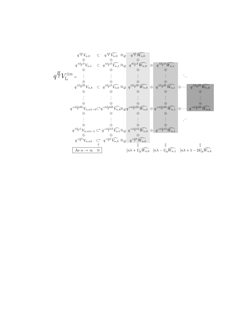
Figure 1. This diagram explains how to compute the desired limit. In the diagram, every representations are understood as taking specialization $\lambda=\alpha-1$. The notation $\subset^{*}$ means that we regard $V_{n,n\lambda-i}$ as sub module of $\widehat{V_{n,i}}$, by using isomorphism $V_{n,n\lambda-i}\cong V_{n,i}$ in Lemma 2.5.

Since $V_{n,i}|_{\lambda=\alpha-1}=0$ if $i>n\lambda=n(\alpha-1)$, by (2.7), as a $\mathbb{L}B_{n}$-module $V_{\mathbb{L}}^{\otimes n}\cong\bigoplus_{i=0}^{n\lambda}V_{n,i}$. Moreover, $q^{\frac{H}{2}}$ acts on $V_{n,i}$ as a scalar multiple by $q^{\frac{n\lambda-2i}{2}}$, so

$$\operatorname{tr}(q^{\frac{H}{2}}\varphi_{\mathbb{L}}(\beta)|_{\lambda=\alpha-1})=\sum_{i=0}^{n\lambda}q^{\frac{n\lambda-2i}{2}}\operatorname{tr}(\varphi^{V}_{n,i}(\beta)|_{\lambda=\alpha-1}).$$

By Lemma 2.5, we identify the braid group representation $V_{n,n\lambda-k}$ as $V_{n,k}$ for $k\leq\frac{n\lambda}{2}$, and then regard each $V_{n,i}$ as a sub $\mathbb{L}B_{n}$-module of $\widehat{V_{n,i}}$. Recall that $\operatorname{tr}(\varphi^{V}_{n,i}(\beta)|_{\lambda=\alpha-1})$ is equal to $\operatorname{tr}(\widehat{\varphi^{V}_{n,i}}(\beta)|_{\lambda=\alpha-1})$ when $\alpha$ is treated as independent variable. By (2.6), over quotient field, $\widehat{V_{n,i}}$ splits as $\bigoplus_{m=0}^{i}\widehat{W_{n,m}}$, hence

$$\operatorname{tr}(\widehat{\varphi^{V}_{n,i}}(\beta)|_{\lambda=\alpha-1})=\sum_{m=0}^{\min\{m,n\lambda-m\}}tr(\widehat{\varphi^{W}_{n,m}}(\beta)|_{\lambda=\alpha-1})$$

This shows

$$\sum_{i=0}^{\alpha-1}q^{\frac{n\lambda-2i}{2}}\operatorname{tr}(\widehat{\varphi^{V}_{n,i}}(\beta)|_{\lambda=\alpha-1}) = \sum_{i=0}^{\alpha-1}q^{\frac{n\lambda-2i}{2}}\sum_{m=0}^{\min\{m,n\lambda-m\}}\operatorname{tr}(\widehat{\varphi^{W}_{n,i}}(\beta)|_{\lambda=\alpha-1})$$

$$= \sum_{m=0}^{\frac{n\lambda}{2}}\sum_{i=m}^{n\lambda-m}q^{\frac{n\lambda-2i}{2}}\operatorname{tr}(\widehat{\varphi^{W}_{n,m}}(\beta)|_{\lambda=\alpha-1})$$

$$= \sum_{m=0}^{\frac{n\lambda}{2}}[n\lambda+1-2m]_{q}\operatorname{tr}(\widehat{\varphi^{W}_{n,m}}(\beta)|_{\lambda=\alpha-1})$$

By Theorem 2.3, when we treat $\alpha$ as independent variable,

$$\operatorname{tr}(\widehat{\varphi^{W}_{n,i}}(\beta))=\operatorname{tr}(L_{n,m}(\beta)|_{x=z^{-1}q,d=-q})$$

hence

$$\lim_{\begin{subarray}{c}\alpha\to\infty\\ \hbar\alpha:\textrm{constant}\end{subarray}}\!\!\!\!\operatorname{tr}(q^{\frac{H}{2}}\circ\varphi_{\mathbb{L}}(\beta)|_{\lambda=\alpha-1}) = \lim_{\begin{subarray}{c}\alpha\to\infty\\ \hbar\alpha:\textrm{constant}\end{subarray}}\!\!\!\!\sum_{m=0}^{\min\{m,n\lambda-m\}}[n\lambda+1-2m]_{q}\operatorname{tr}(L_{n,m}(\beta)|_{x=z^{-1}q,d=-q})$$

$$= \sum_{m=0}^{\infty}\frac{z^{\frac{n}{2}}q^{\frac{1}{2}(1-n-2m)}-z^{-\frac{n}{2}}q^{-\frac{1}{2}(1-n-2m)}}{q^{\frac{1}{2}}-q^{-\frac{1}{2}}}\operatorname{tr}(L_{n,m}(\beta)|_{x=z^{-1}q,d=-q}).$$

Therefore we conclude

$$CJ_{K}(\hbar,z)=\frac{z^{-\frac{1}{2}e(\beta)}q^{\frac{1}{2}e(\beta)}}{z^{\frac{1}{2}}-z^{-\frac{1}{2}}}\sum_{m=0}^{\infty}(z^{\frac{n}{2}}q^{\frac{1}{2}(1-n-2m)}-z^{-\frac{n}{2}}q^{-\frac{1}{2}(1-n-2m)})\operatorname{tr}(L_{n,m}(\beta)|_{x=z^{-1}q,d=-q}).$$

∎

As we have mentioned, Theorem 3.1 provides an alternative, direct method to compute the loop expansion of the colored Jones polynomial although actual computation may be quite hard, since one should know $L_{n,m}(\beta)$ for all $m$. Here we give sample calculations.

Example 3.2 (Unknot).

Let us consider the unknot $K$ represented as a closure of 2-braid $\sigma_{1}$. The trace of Lawrence’s representation is given by $\operatorname{tr}L_{2,m}(\sigma_{1})=(-x)^{m}(-d)^{\binom{m}{2}}$ so

$$CJ_{\textsf{Unknot}}(z,\hbar) = \frac{z^{-\frac{1}{2}}q^{\frac{1}{2}}}{z^{\frac{1}{2}}-z^{-\frac{1}{2}}}\sum_{m=0}^{\infty}(zq^{\frac{-1-2m}{2}}-z^{-1}q^{\frac{1+2m}{2}})(-z)^{-m}q^{\binom{m+1}{2}}$$

$$= \frac{z^{-\frac{1}{2}}q^{\frac{1}{2}}}{z^{\frac{1}{2}}-z^{-\frac{1}{2}}}(zq^{-\frac{1}{2}}-q^{-\frac{1}{2}})$$

$$= 1.$$

Example 3.3 ($(2,p)$-torus knot).

More generally, let us consider $(2,p)$-torus knot $T(2,p)$ represented as a closure of 2-braid $\sigma_{1}^{p}$. The trace of Lawrence’s representation is given by $\operatorname{tr}L_{2,m}(\sigma_{1}^{p})=(-x^{p})^{m}(-d^{p})^{\binom{m}{2}}$ so

(3.1) $$CJ_{T(2,p)}(z,\hbar)=\frac{z^{-\frac{1}{2}p}q^{\frac{1}{2}p}}{z^{\frac{1}{2}}-z^{-\frac{1}{2}}}\sum_{m=0}^{\infty}(zq^{\frac{-1-2m}{2}}-z^{-1}q^{\frac{1+2m}{2}})(-z^{-p})^{m}q^{\binom{m+1}{2}p}$$

To compute the $1$-loop part, let us put $\hbar=0$. Then

$$V^{(0)}_{T(2,p)}(z) = \frac{z^{-\frac{1}{2}p}}{z^{\frac{1}{2}}-z^{-\frac{1}{2}}}\sum_{m=0}^{\infty}(z-z^{-1})(-z^{-p})^{m}=(z^{\frac{1}{2}}+z^{-\frac{1}{2}})z^{-\frac{p}{2}}\sum_{m=0}^{\infty}(-z^{-p})^{m}$$

$$= (z^{\frac{1}{2}}+z^{-\frac{1}{2}})z^{-\frac{p}{2}}\frac{1}{1+z^{-p}}$$

$$= \frac{z^{\frac{1}{2}}+z^{-\frac{1}{2}}}{z^{\frac{1}{2}p}+z^{-\frac{1}{2}p}}$$

which is equal the inverse of the Alexander-Conway polynomial of $T(2,p)$.

Next let us compute the 2-loop part. By putting $q=e^{\hbar}$ and looking at the coefficient of $\hbar$ in (3.1), we have

$$V^{(1)}_{T(2,p)}(z) = \frac{z^{-\frac{1}{2}p}}{z^{\frac{1}{2}}-z^{-\frac{1}{2}}}\left(\frac{z}{2}\sum_{m=0}^{\infty}[pm^{2}+(p-2)m+(p-1)](-z^{-pm})\right.$$

$$\ \ \ \ \ \ \ \ \ \ \ \ \ \ \ \left.-\frac{z^{-1}}{2}\sum_{m=0}^{\infty}[pm^{2}+(p+2)m+(p+1)](-z^{-pm})\right)$$

In the ring of formal power series $\mathbb{C}[[z,z^{\pm 1}]]$, we have

$$\sum_{m=0}^{\infty}z^{m}=\frac{1}{1-z},\ \sum_{m=0}^{\infty}mz^{m}=\frac{z}{(1-z)^{2}},\ \sum_{m=0}^{\infty}m^{2}z^{m}=\frac{z+z^{2}}{(1-z)^{3}}.$$

Hence

$$V^{(1)}_{T(2,p)}(z)=\frac{1}{(z^{\frac{1}{2}}-z^{-\frac{1}{2}})(z^{\frac{1}{2}p}+z^{-\frac{1}{2}p})^{3}}\left((p-1)z^{p+1}-(p+1)z^{p-1}+(p+1)z^{-p+1}-(p-1)z^{-p-1}\right).$$

For example,

$$V^{(1)}_{T(2,3)}(z)=\frac{(z^{4}-2z^{2}+2-2z^{-2}+z^{-4})}{\Delta_{T(2,3)}(z)^{3}}=\frac{(z^{4}-2z^{2}+2-2z^{-2}+z^{-4})}{(z-1+z^{-1})^{3}}.$$

Now it is a direct consequence that the 1-loop part is the inverse of the Alexander-Conway polynomial.

Corollary 3.4 (Melvin-Morton-Ronzansky conjecture).

$$V^{(0)}(z)=\frac{1}{\Delta_{K}(z)}$$

Proof.

The $1$-loop part $V^{(0)}(z)$ is obtained by putting $\hbar=0$ in the formula of Theorem 3.1. Since $d=-q=-e^{\hbar}$, in a homological representation, putting $\hbar=0$ corresponds to putting $d=-1$. As we have pointed out in Proposition 2.2,

$$L_{n,m}(\beta)|_{d=-1}=\operatorname{Sym}^{m}L_{n,1}(\beta).$$

Therefore, by Theorem 3.1, the $1$-loop part $V^{(0)}(z)$ is written as

$$V^{(0)}(z) = z^{-\frac{1}{2}e(\beta)}\frac{z^{\frac{n}{2}}-z^{-\frac{n}{2}}}{z^{\frac{1}{2}}-z^{-\frac{1}{2}}}\sum_{i=0}^{\infty}\operatorname{tr}L_{n,i}(\beta)|_{x=z^{-1},d=-1}$$

$$= z^{-\frac{1}{2}e(\beta)}\frac{z^{\frac{n}{2}}-z^{-\frac{n}{2}}}{z^{\frac{1}{2}}-z^{-\frac{1}{2}}}\sum_{i=0}^{\infty}\operatorname{tr}(\operatorname{Sym}^{i}L_{n,1})(\beta)|_{x=z^{-1}}.$$

MacMahon Master Theorem says that

$$\sum_{i=0}^{\infty}\operatorname{tr}(\operatorname{Sym}^{i}L_{n,1})(\beta)=\det(I-L_{n,1}(\beta))^{-1}$$

hence

$$V^{(0)}(z)=z^{-\frac{1}{2}e(\beta)}\frac{z^{\frac{n}{2}}-z^{-\frac{n}{2}}}{z^{\frac{1}{2}}-z^{-\frac{1}{2}}}\frac{1}{\det(I-L_{n,1}(\beta)|_{x=z^{-1}})}=\frac{1}{\Delta_{K}(z^{-1})}=\frac{1}{\Delta_{K}(z)}.$$

∎

4. Entropy and colored Jones polynomials

In this section we give an application of topological interpretation of quantum representations.

4.1. Entropy estimates from configuration space

For a homeomorphism of a compact topological space or a metric space $f:X\rightarrow X$, there is a fundamental numerical invariant $h(f)\in\mathbb{R}$ of topological dynamics called the (topological) entropy.

Let $\overline{C}_{m}(X)$ and $C_{m}(X)$ be the ordered and unordered configuration space of $m$-points of $X$,

$$\overline{C}_{m}(X)=\{(x_{1}\ldots,x_{m})\in X^{m}\>|\>x_{i}\neq x_{j}\},\ \ C_{m}(X)=\overline{C}_{m}(X)/S_{m}$$

where $S_{m}$ is the symmetric group that acts as permutations of the coordinates. Then $f$ induces the continuous maps $\overline{C}_{m}(f):\overline{C}_{m}(X)\rightarrow\overline{C}_{m}(X)$ and $C_{m}(f):C_{m}(X)\rightarrow C_{m}(X)$, respectively.

Note that $\overline{C}_{m}(X)\subset X^{m}$ is invariant under $f^{\times m}:X^{m}\rightarrow X^{m}$ so

$$h(\overline{C}_{m}(f))\leq h(f^{\times m})=mh(f).$$

The unordered configuration space $\overline{C}_{m}(X)$ is a finite cover of $C_{m}(X)$ so $h(C_{m}(f))=h(\overline{C}_{m}(f))$.

Now for $A\in\textrm{GL}(n;\mathbb{C})$ let $\rho(A)$ be its spectral radius of $A$, the maximum of the absolute value of the eigenvalues of $A$. It is known that if $C_{m}(f)$ is nice enough (see [Fr], for sufficient conditions for inequality (4.1) to hold), then spectral radius of the induced action on homology provides a lower bound of the entropy

(4.1) $$\log\rho(C_{m}(f)_{*}:H_{*}(C_{m}(f),\mathbb{Z})\rightarrow H_{*}(C_{m}(f),\mathbb{Z}))\leq h(C_{m}(f)).$$

Hence if $f$ is good enough, by using configuration spaces we have an estimate of entropy

(4.2) $$\log\rho(C_{m}(f)_{*})\leq mh(f).$$

The above considerations nicely fit for the braid groups. Let us regard the braid group $B_{n}$ as the mapping class group of $n$-punctured disc $D_{n}$. The entropy of braid $\beta\in B_{n}$ is defined by the infimum of entropy of homeomorphisms representing $\beta$,

$$h(\beta)=\inf\{h(f)\>|f:D_{n}\rightarrow D_{n},[f]=\beta\in MCG(D_{n})=B_{n}\}.$$

By Nielsen-Thurston classification [FLP, Th], there is a representative homeomorphism $f_{\beta}$ that attains the infimum so $h(\beta)=h(f_{\beta})$. In particular, if $\beta$ is pseudo-Anosov, then a psuedo-Anosov representative attains the infimum. By abuse of notation, we will use the same symbol $\beta$ to mean its representative homeomoprhism $f_{\beta}$ that attains the infimum of the entropy.

As Koberda shows in [Kob], the inequality (4.1) holds in the case $X$ is surface. This implies that Lawrence’s representation gives an estimate of entropy.

Theorem 4.1.

For an $n$-braid $\beta$,

$$\sup_{|x|=1,|d|=1}\log\rho(L_{n,m}(\beta))\leq mh(\beta)$$

Proof.

Let $\widetilde{C}$ be a finite covering of the unordered configuration space $C_{n,m}=C_{m}(D_{n})$. If the action of $\beta$ on $C_{n,m}$ lifts, then by (4.2), $\log\rho(\widetilde{\beta_{\widetilde{C}}}{}_{*})\leq mh(\beta)$ holds, where $\widetilde{\beta_{\widetilde{C}}}:\widetilde{C}\rightarrow\widetilde{C}$ denotes the lift of a homeomorphism $\beta$.

For non-negative integers $A,B$, Let $\widetilde{C}=\widetilde{C}_{A,B}$ be a finite abelian covering of $C_{n,m}$ that corresponds to the kernel of $\alpha_{A,B}:\pi_{1}(C_{n,m})\rightarrow\mathbb{Z}/A\mathbb{Z}\oplus\mathbb{Z}/B\mathbb{Z}$, where $\alpha_{A,B}$ is given by the compositions

The standard topological argument, using the eigenspace decompositions for the deck translations (See [BB] for the case $\mathbb{Z}$-covering, the case of the reduced Burau representation $L_{n,1}$. The same argument applies to the case $\mathbb{Z}^{2}$-covering) shows that for $a=1,\ldots,A-1$ and $b=1,\ldots,B-1$,

$$\rho(L_{n,m}(\beta)|_{x=e^{\frac{2\pi a\sqrt{-1}}{A}},d=e^{\frac{2\pi b\sqrt{-1}}{B}}})\leq\rho(\widetilde{\beta}_{\widetilde{C}_{A,B}}).$$

The sets $\{(e^{\frac{2\pi a\sqrt{-1}}{A}},e^{\frac{2\pi b\sqrt{-1}}{B}})\in\>|\>A,a,B,b\in\mathbb{Z}\}$ is dense in $S^{1}\times S^{1}=\{(x,d)\in\mathbb{C}^{2}\>|\>|x|=|d|=1\}$, hence we get desired inequality. ∎

Since generically one can identify the quantum representation with Lawrence’s representation, quantum representations also provide estimates of entropy.

Theorem 4.2.

Let $\beta$ be an $n$-braid.

1. $\sup_{|q|=1,|z|=1}\log\rho(\widehat{\varphi_{n,m}^{W}}(\beta))\leq mh(\beta)$.

2. $\sup_{|q|=1,|z|=1}\log\rho(\widehat{\varphi_{n,m}^{V}}(\beta))\leq mh(\beta)$.

3. $\sup_{|q|=1}\log\rho(\varphi_{\alpha}(\beta))\leq\frac{n\alpha-n}{2}h(\beta)$.

Proof.

The assertions (1) and (2) follows from Theorem 4.1 and Theorem 2.3. To see (3), recall that as a $\mathbb{L}B_{n}|_{z=q^{\alpha-1}}=\mathbb{C}[q^{\pm 1}]B_{n}$-module, we have

$$V_{\alpha}^{\otimes n}\cong V_{\mathbb{L}}|_{z=q^{\alpha-1}}\subset\bigoplus_{m=0}^{n(\alpha-1)}V_{n,m}|_{\lambda=\alpha-1}.$$

Moreover, by Lemma 2.5 $V_{n,m}|_{\lambda=\alpha-1}\cong V_{n,n(\alpha-1)-m}|_{\lambda=\alpha-1}$. Therefore,

$$\sup_{|q|=1}\rho(\varphi_{\alpha}(\beta))\leq\max_{1\leq m\leq\frac{n(\alpha-1)}{2}}\sup_{|q|=1}(\varphi^{V}_{n,m}(\beta)|_{z=q^{\alpha-1}})\leq\max_{1\leq m\leq\frac{n(\alpha-1)}{2}}\sup_{|q|=1}\rho(\widehat{\varphi^{V}_{n,m}}(\beta)|_{z=q^{\alpha-1}}).$$

By (1), we conclude

$$\sup_{|q|=1}\log\rho(\varphi_{\alpha}(\beta))\leq\frac{n(\alpha-1)}{2}h(\beta).$$

∎

4.2. Quantum $\mathfrak{sl}_{2}$ invariants and entropy

An estimates in Theorem 4.2 suggests a new relationship between quantum invariants and entropy of braids.

For $\alpha\in\{2,3\ldots,\}$, let $Q^{\mathfrak{sl}_{2};V_{\alpha}}_{K}(q)=\operatorname{tr}(q^{\frac{H}{2}}\varphi_{\alpha}(\beta))=[\alpha]_{q}J_{\alpha,K}(q)$ be the quantum $(\mathfrak{sl}_{2},V_{\alpha})$-invariant of the knot $K$, another common normalization of the colored Jones polynomials used to define quantum invariants of 3-manifolds.

Theorem 4.3.

Let $K$ be a knot represented as the closure of an $n$-braid $\beta$, and $\alpha\in\{2,3,\ldots\}$. Then

$$\sup_{|q|=1}\log|Q^{\mathfrak{sl}_{2};V_{\alpha}}_{K}(q)|\leq n\log\alpha+\log\rho(\varphi_{\alpha}(\beta))\leq n\log\alpha+\frac{n(\alpha-1)}{2}h(\beta).$$

Proof.

By definition of the spectral radius,

$$|Q^{\mathfrak{sl}_{2};V_{\alpha}}_{K}(q)|=|\operatorname{tr}(q^{\frac{H}{2}}\varphi_{\alpha}(\beta))|\leq\alpha^{n}\rho(q^{\frac{H}{2}}\varphi_{\alpha}(\beta))\leq\alpha^{n}\rho(q^{\frac{H}{2}})\rho(\varphi_{\alpha}(\beta)).$$

Here the last inequality follows from the fact that $q^{\frac{H}{2}}$ and $\varphi_{\alpha}(\beta)$ commutes. When $|q|=1$, $\rho(q^{\frac{H}{2}})=1$ hence by Theorem 4.2 (3), we conclude

$$\sup_{|q|=1}|\operatorname{tr}(q^{\frac{H}{2}}\varphi_{\alpha}(\beta))|\leq\sup_{|q|=1}\alpha^{n}\rho(\varphi_{\alpha}(\beta))\leq\alpha^{n}e^{\frac{n(\alpha-1)}{2}h(\beta)}.$$

∎

By an analogy of the famous volume conjecture [Ka, MuMu], It is interesting to look at the asymptotic behavior of $|Q^{\mathfrak{sl}_{2};V_{\alpha}}_{K}(q)|$. By Theorem 4.3, we have

$$\frac{\sup_{|q|=1}\log|Q^{\mathfrak{sl}_{2};V_{\alpha}}_{K}(q)|}{\alpha}\leq n\frac{\log\alpha}{\alpha}+\frac{\sup_{|q|=1}\log\rho(\varphi_{\alpha}(\beta))}{\alpha}\leq n\frac{\log\alpha}{\alpha}+\frac{n(\alpha-1)}{2\alpha}h(\beta)$$

This shows

(4.3) $$\limsup_{\alpha\to\infty}\frac{\sup_{|q|=1}\log|Q^{\mathfrak{sl}_{2};V_{\alpha}}_{K}(q)|}{\alpha}\leq\limsup_{\alpha\to\infty}\frac{\sup_{|q|=1}\log\rho(\varphi_{\alpha}(\beta))}{\alpha}\leq\frac{n}{2}h(\beta).$$

It is interesting to ask the convergence of the limits and when the inequalities (4.3) yield the equalities. In particular, the second inequlaity is related to the question when the estimation of entropy from quantum representation is asymptotically sharp.

A. Appendix: Multiforks for Lawrence’s representation $L_{n,m}$

In this appendix, we present multiforks in Lawrence’s representation $L_{n,m}$ and explicit matrices of $L_{n,m}(\sigma_{i})$. For the basics of geometric treatments of Lawrence’s representation, see [I, Section 2].

First we review the definition of multiforks and how multifork represent a homology class in $H^{lf}_{m}(\widetilde{C_{m,n}};\mathbb{Z})$. Let $Y$ be the $Y$-shaped graph with four vertices $c,r,v_{1},v_{2}$ and oriented edges as shown in Figure 2(1). A fork $F$ based on $d\in\partial D_{n}$ is an embedded image of $Y$ into $D^{2}=\{z\in\mathbb{C}\>|\>|z|\leqslant n+1\}$ such that:

• All points of $Y\setminus\{r,v_{1},v_{2}\}$ are mapped to the interior of $D_{n}$.

• The vertex $r$ is mapped to $d_{i}$.

• The other two external vertices $v_{1}$ and $v_{2}$ are mapped to the puncture points.

The image of the edge $[r,c]$ and the image of $[v_{1},v_{2}]=[v_{1},c]\cup[c,v_{2}]$ regarded as a single oriented arc, are denoted by $H(F)$ and $T(F)$. We call $H(F)$ and $T(F)$ the handle and the tine of the fork $F$, respectively.

A multifork of dimension $m$ is an ordered tuples of $m$ forks $\mathbb{F}=(F_{1},\ldots,F_{m})$ such that

• $F_{i}$ is a fork based on $d_{i}$.

• $T(F_{i})\cap T(F_{j})\cap D_{n}=\emptyset$ $(i\neq j)$.

• $H(F_{i})\cap H(F_{j})=\emptyset$ $(i\neq j)$.

Figure 2 (2) illustrates an example of a multifork of dimension $3$. We often use to represent multiforks consisting of $k$ parallel forks by drawing single fork labelled by $k$, as shown in Figure 2 (3).

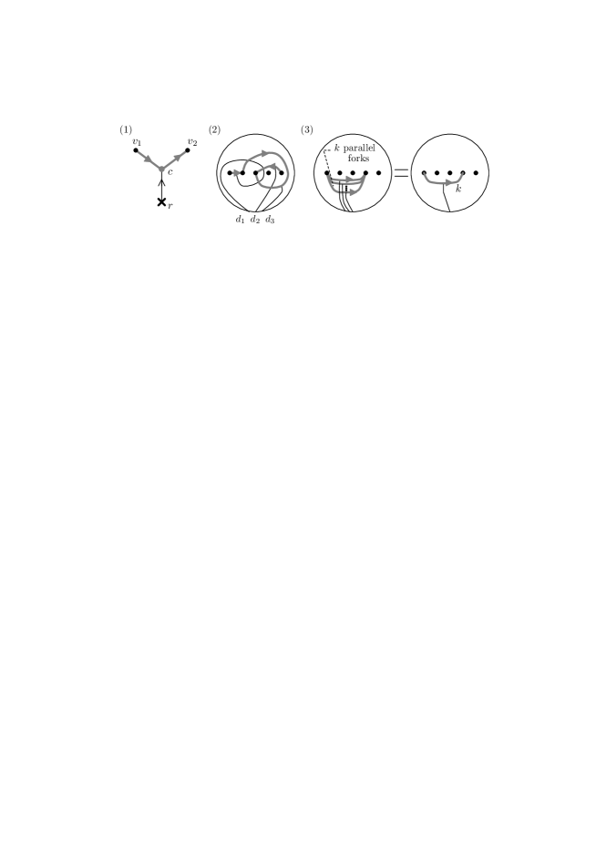
Figure 2. Multiforks: to distinguish tines and handle, we often write tine of forks by a bold gray line.

For a multifork $\mathbb{F}$, we regard the handle $H(F_{i})$ of the fork $F_{i}$ as a path $\gamma_{i}\colon\thinspace[0,1]\rightarrow D_{n}$ in $D_{n}$ by taking an appropriate parametrization. Then the handles of $\mathbb{F}$ defines a path $H(\mathbb{F})=\{\gamma_{1},\ldots,\gamma_{m}\}\colon\thinspace[0,1]\rightarrow C_{n,m}$ in $C_{n,m}$. Take a lift of $H(\mathbb{F})$, $\widetilde{H(\mathbb{F})}\colon\thinspace[0,1]\rightarrow\widetilde{C}_{n,m}$ so that $\widetilde{H(\mathbb{F})}(0)=\widetilde{\mathbf{d}}$.

Let $\Sigma(\mathbb{F})=\left\{\{z_{1},\ldots,z_{m}\}\in C_{n,m}\>|\>z_{i}\in T(F_{i})\right\}$, and $\widetilde{\Sigma}(\mathbb{F})$ be the $m$-dimensional submanifold of $\widetilde{C}_{n,m}$ which is the connected component of $\pi^{-1}(\Sigma(\mathbb{F}))$ containing $\widetilde{H(\mathbb{F})}(1)$. The submanifold $\widetilde{\Sigma}(\mathbb{F})$ defines an element of $H_{m}^{lf}(\widetilde{C}_{n,m};\mathbb{Z})$. By abuse of notation, we will use $\mathbb{F}$ to represent both multifork and the homology class $[\widetilde{\Sigma}(\mathbb{F})]\in H_{m}^{lf}(\widetilde{C}_{n,m};\mathbb{Z})$.

Here the orientation of $\widetilde{\Sigma}(\mathbb{F})$ is defined so that a canonical homeomorphism $T(F_{1})\times\cdots\times T(F_{m})\rightarrow\Sigma(\mathbb{F})$ is orientation preserving. Thus, for a fork $\mathbb{F}_{\tau}=(F_{\tau(1)},\cdots,F_{\tau(m)})$ obtained by permuting its coordinate by a permutation $\tau\in S_{m}$, we have $\mathbb{F}_{\tau}=\textsf{sgn}(\tau)\mathbb{F}\in H_{m}^{lf}(\widetilde{C}_{n,m};\mathbb{Z})$.

For $\mathbf{e}=(e_{1},\ldots,e_{n-1})\in E_{n,m}$, we assign a multifork $\mathbb{F}_{\mathbf{e}}=\{F_{1},\ldots,F_{m}\}$ in Figure 3 and call $\mathbb{F}$ a standard multifork.

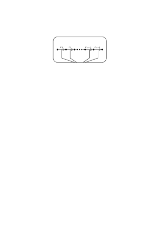
Figure 3. Standard multifork $\mathbb{F}_{\mathbf{e}}$ for $\mathbf{e}=(e_{1},\ldots,e_{n-1})$

The set of standard multiforks spans a $\mathbb{Z}[x^{\pm 1},d^{\pm 1}]$-submodule $\mathcal{H}_{n,m}$ of $H_{m}^{lf}(\widetilde{C_{n,m}};\mathbb{Z})$, which is free of dimension $\binom{n+m-2}{2}$ and is invariant under the $B_{n}$-action. This defines a (geometric) Lawrence’s representation $L_{n,m}:B_{n}\rightarrow\textrm{GL}\left(\binom{n+m-2}{2};\mathbb{Z}[x^{\pm 1},d^{\pm 1}]\right).$

From the definition of the submanifold $\widetilde{\Sigma}(\mathbb{F})$, we graphically express several relations among homology classes represented by multifork, which allows us to express a given multifork as a sum of standard multiforks (see [Kra, Big2] for the case $m=2$).

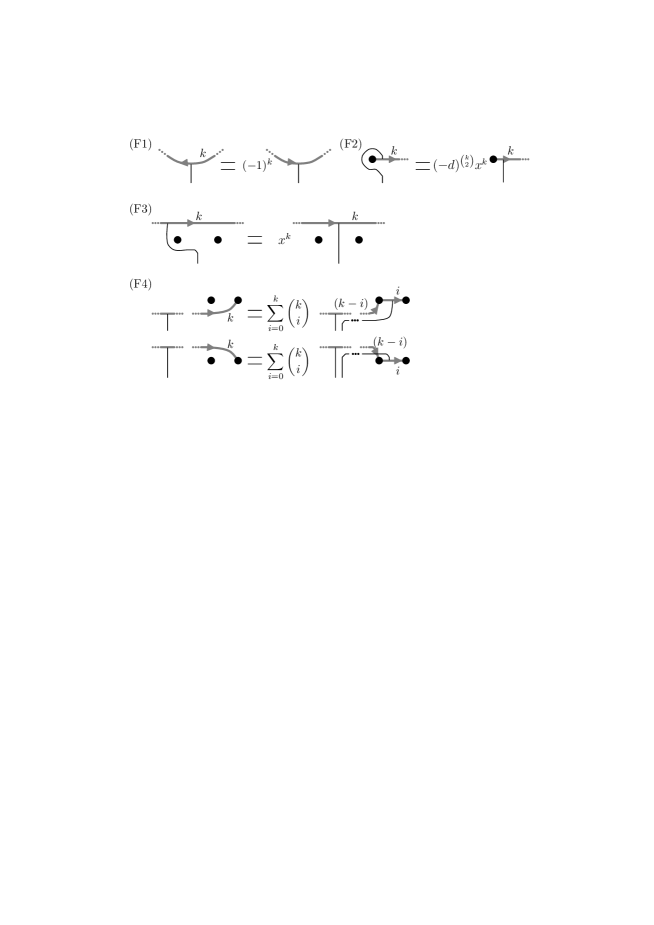
Figure 4. Geometric rewriting formula for multiforks

In particular, these formulae leads to a formula of an explicit matrix representative of $L_{n,m}(\sigma_{i})$:

(A.1) $$L_{n,m}(\sigma_{1})(\mathbb{F}_{e_{1},\ldots,e_{n-1}}) =\sum_{l=0}^{e_{2}}(-1)^{e_{1}}(-d)^{\binom{e_{1}}{2}}x^{e_{1}}\binom{e_{2}}{l}\mathbb{F}_{e_{1}+e_{2}-l,l,\ldots}$$

$$L_{n,m}(\sigma_{i})(\mathbb{F}_{e_{1},\ldots,e_{n-1}}) =\sum_{k=0}^{e_{i-1}}\sum_{l=0}^{e_{i+1}}(-1)^{e_{i}}(-d)^{\binom{e_{i}+k}{2}}x^{e_{i}+k}\binom{e_{i-1}}{k}\binom{e_{i+1}}{l}\mathbb{F}_{\ldots,e_{i-1}-k,e_{i}+k+e_{i+1}-l,l,\ldots}$$

$$\hskip 113.81102pt(i=2,\ldots,n-2)$$

$$L_{n,m}(\sigma_{n-1})(\mathbb{F}_{e_{1},\ldots,e_{n-1}}) =\sum_{k=0}^{e_{n-2}}(-1)^{e_{n-1}}(-d)^{\binom{e_{n-1}+k}{2}}x^{e_{n-1}+k}\binom{e_{n-2}}{k}\mathbb{F}_{\ldots,e_{n-2}-k,e_{n-1}+k}$$

As we already mentioned, Proposition 2.2 follows from formula (A.1).

However, a multifork expression gives a direct way to see Proposition 2.2: First note that by orientation convention of $\widetilde{\Sigma}(\mathbb{F})$, when $d=-1$, the homology class represented by a multifork $\mathbb{F}=(F_{1},\ldots,F_{m})$ is independent of a choice of indices of forks, namely, for a fork $\mathbb{F}_{\tau}=(F_{\tau(1)},\ldots,F_{\tau(m)})$ obtained by permuting its coordinate by a permutation $\tau\in S_{m}$, $\mathbb{F}_{\tau}=\mathbb{F}$. Therefore, the correspondence between multifork $\mathbb{F}=(F_{1},\ldots,F_{m})$ that represents an element of $\mathcal{H}_{n,m}$ and a family of $m$ forks $\{F_{1},\ldots,F_{k}\}$ that represents an element of $\operatorname{Sym}^{m}\mathcal{H}_{n,1}$ gives rise to the desired isomorphism $\mathcal{H}_{n,m}\rightarrow\operatorname{Sym}^{m}\mathcal{H}_{n,1}$.

References

- [BG] D. Bar-Natan and S. Garoufalidis, On the Melvin-Morton-Rozansky conjecture, Invent. Math, 125, (1996), 103–133.
- [BB] G. Band and P. Boyland, The Burau estimate for the entropy of a braid, Algebr. Geom. Topol. 7 (2007), 1345–1378.
- [Big1] S. Bigelow, Braid groups are linear, J. Amer. Math. Soc. 14, (2000), 471–486.
- [Big2] S. Bigelow, A homological definition of the Jones polynomial, Invariants of knots and 3-manifolds (Kyoto, 2001), 29–41, Geom. Topol. Monogr., 4, Geom. Topol. Publ., Coventry, 2002.
- [FLP] A. Fathi, F. Laudenbach, and V. Poénaru, Travaux de Thurston sur les surfaces, Astẃrisque, 66-67. Société Mathématique de France, Paris, 1979. 284 pp.
- [Fr] D. Fried, Entropy and twisted cohomology, Topology, 25 (1986), 455–470.
- [GK] S. Garoufalidis and A. Kricker, A rational noncommutative invariant of boundary links, Geom. Topol. 8 (2004) 115–204.
- [GR] S. Garoufalidis and L. Rozansky, The loop expansion of the Kontsevich integral, the null-move and S-equivalence, Topology 43, (2004), 1183–1210.
- [Ha] K. Habiro, Claspers and finite type invariants of links, Geom. Topol. 4 (2000), 1–83.
- [I] T. Ito, Reading the dual Garside length of braids from homological and quantum representations, Comm. Math. Phys. to appear.
- [JK] C. Jackson and T. Kerler, The Lawrence-Krammer-Bigelow representations of the braid groups via , Adv. Math, 228, (2011), 1689–1717.
- [Ka] R. Kashaev, The hyperbolic volume of knots from the quantum dilogarithm Lett. Math. Phys. 39 (1997) 269–275.
- [Kas] C. Kassel, Quantum groups, Graduate Texts in Mathematics 155. Springer-Verlag, New York, 1995.
- [Kob] T. Koberda, Asymptotic linearity of the mapping class group and a homological version of the Nielsen-Thurston classification, Geom. Dedicata 156 (2012), 13–30.
- [Koh] T. Kohno, Quantum and homological representations of braid groups,Configuration Spaces - Geometry, Combinatorics and Topology, Edizioni della Normale (2012), 355–372.
- [Kra] D. Krammer, The braid group is linear, Invent. Math. 142, (2000), 451–486.
- [Kra2] D. Krammer, Braid groups are linear, Ann. Math. 155, (2002), 131–156.
- [Kri] A. Kricker, The lines of the Kontsevich integral and Rozansky’s rationality conjecture, arXiv:math.GT/0005284.
- [La] R. Lawrence, Homological representations of the Hecke algebra, Comm. Math. Phys. 135, (1990), 141–191.
- [La2] R. Lawrence, A functorial approach to the one-variable Jones polynomial, J. Differential Geom. 37 (1993), 689–710.
- [MeMo] P. Melvin and H. Morton , The coloured Jones function, Comm. Math. Phys. 169, (1995), 501–520.
- [MuMu] H. Murakami, and J. Murakami, The colored Jones polynomials and the simplicial volume of a knot, Acta Math. 186 (2001), 85–104.
- [Oh1] T. Ohtsuki, A cabling formula for the 2-loop polynomial of knots, Publ. Res. Inst. Math. Sci. 40 (2004), 949–971.
- [Oh2] T. Ohtsuki, On the 2-loop polynomial of knots, Geom. Topol. 11 (2007), 1357–1475.
- [Ro1] L. Ronzansky, The universal R-matrix, Burau representation, and the Melvin-Morton expansion of the colored Jones polynomial, Adv. Math 134 (1998), 1–31.
- [Ro2] L. Ronzansky, A rationality conjecture about Kontsevich integral of knots and its implications to the structure of the colored Jones polynomial, Topology Appl. 127 (2003), 47–76.
- [Th] W. Thurston, On the geometry and dynamics of diffeomorphisms of surfaces, Bull. Amer. Math. Soc. 19 (1988), 417–431.