Stochastic Block Transition Models for
Dynamic Networks

Abstract

There has been great interest in recent years on statistical models for dynamic networks. In this paper, I propose a stochastic block transition model (SBTM) for dynamic networks that is inspired by the well-known stochastic block model (SBM) for static networks and previous dynamic extensions of the SBM. Unlike most existing dynamic network models, it does not make a hidden Markov assumption on the edge-level dynamics, allowing the presence or absence of edges to directly influence future edge probabilities while retaining the interpretability of the SBM. I derive an approximate inference procedure for the SBTM and demonstrate that it is significantly better at reproducing durations of edges in real social network data.

1 Introduction

Analysis of data in the form of networks has been a topic of interest across many disciplines, aided by the development of statistical models for networks. Many models have been proposed for static networks, where the data consist of a single observation of the network (Goldenberg et al., 2009). On the other hand, modeling dynamic networks is still in its infancy; much research on dynamic network modeling has appeared only in the past several years. Statistical models for static networks typically utilize a latent variable representation for the network; such models have been extended to dynamic networks by allowing the latent variables, which I refer to as states, to evolve over time.

This paper targets networks evolving in discrete time in which both nodes and edges can appear and disappear over time, such as dynamic networks of social interactions. Most existing dynamic network models assume a hidden Markov structure, where a snapshot of the network at any particular time is conditionally independent from all previous snapshots given the current network states. Such an approach greatly simplifies the model and allows for tractable inference, but it may not be flexible enough to replicate certain observations from real network data, such as time durations of edges, which are often inaccurately reproduced by models with hidden Markov dynamics.

In this paper I propose a stochastic block transition model (SBTM) for dynamic networks, inspired by the well-known stochastic block model (SBM) for static networks. The approach generalizes two recent dynamic extensions of SBMs that utilize the hidden Markov assumption (Yang et al., 2011; Xu and Hero III, 2014). In the SBTM, the presence (or absence) of an edge between two nodes at any given time step directly influences the probability that such an edge would appear at the next time step.

I demonstrate that, under the SBTM, the sample mean of a scaled version of the observed adjacency matrix at each time is asymptotically Gaussian. Taking advantage of this property, I develop an approximate inference procedure using a combination of an extended Kalman filter and a local search algorithm. I investigate the accuracy of the inference procedure via a simulation experiment. Finally I fit the SBTM to a real dynamic network of social interactions and demonstrate its ability to more accurately replicate edge durations while retaining the interpretability of the SBM.

2 Related Work

There has been significant research dedicated to statistical modeling of dynamic networks, mostly in the past several years. Much of the earlier work is covered in the excellent survey by Goldenberg et al. (2009). Key contributions in this area include dynamic extensions of static network models including exponential random graph models (Guo et al., 2007), stochastic block models (Xing et al., 2010; Ho et al., 2011; Ishiguro et al., 2010; Yang et al., 2011; Xu and Hero III, 2014), continuous latent space models (Sarkar and Moore, 2005; Sarkar et al., 2007; Hoff, 2011; Lee and Priebe, 2011; Durante and Dunson, 2014), and latent feature models (Foulds et al., 2011; Heaukulani and Ghahramani, 2013; Kim and Leskovec, 2013).

Several dynamic extensions of stochastic block models are related to this paper. Xing et al. (2010) and Ho et al. (2011) proposed dynamic extensions of a mixed-membership version of the SBM. Ishiguro et al. (2010) proposed a dynamic extension of the infinite relation model, which is a nonparametric version of the SBM. Yang et al. (2011) and Xu and Hero III (2014) proposed dynamic extensions of the standard SBM; these models are closely related to the model proposed in this paper and are further discussed in Section 3.2.

Most dynamic network models assume a hidden Markov structure. Specifically the network states follow Markovian dynamics, and it is assumed that a network snapshot is conditionally independent of all past snapshots given the current states. While tractable, such an assumption may not be realistic in many settings, including dynamic networks of social interactions. For example, if two people interact with each other at some time, it may influence them to interact again in the near future. Viswanath et al. (2009) reported that over $80\%$ of pairs of Facebook users continued to interact one month after an initial interaction, and over $60\%$ continued after three months, suggesting that such an influence may be present.

In hidden Markov dynamic network models, observing an edge influences the estimated probability of that edge re-occurring in the future only by affecting the estimated states corresponding to the edge, so the influence is weak. A stronger influence can be incorporated by allowing the presence of a future edge to depend both on the current network states and on whether or not an edge is currently present. The model I propose satisfies this property. To the best of my knowledge, the only other dynamic network model satisfying this property is the latent feature propagation model proposed by Heaukulani and Ghahramani (2013).

3 Stochastic Block Models

3.1 Static Stochastic Block Models

A static network is represented by a graph over a set of nodes $\mathcal{V}$ and a set of edges $\mathcal{E}$. The nodes and edges are represented by a square adjacency matrix $W$, where an entry $w_{ij}=1$ denotes that an edge is present from node $i\in\mathcal{V}$ to node $j\in\mathcal{V}\setminus\{i\}$, and $w_{ij}=0$ denotes that no such edge is present. Unless otherwise specified, I assume directed graphs, i.e. $w_{ij}\neq w_{ji}$ in general, with no self-edges, i.e. $w_{ii}=0$. Let $\mathcal{C}=\{\mathcal{C}_{1},\dots,\mathcal{C}_{k}\}$ denote a partition of $\mathcal{V}$ into $k$ classes. I use the notation $i\in a$ to denote that node $i$ belongs to class $a$. I represent the partition by a class membership vector $\boldsymbol{\mathbf{c}}$, where $c_{i}=a$ is equivalent to $i\in a$.

A stochastic block model (SBM) for a static network is defined as follows (adapted from Definition 3 in Holland et al. (1983)):

Definition 1 (Stochastic block model).

Let $W$ denote a random adjacency matrix for a static network, and let $\boldsymbol{\mathbf{c}}$ denote a class membership vector. $W$ is generated according to a stochastic block model with respect to the membership vector $\boldsymbol{\mathbf{c}}$ if and only if,

1. For any nodes $i\neq j$, the random variables $w_{ij}$ are statistically independent.

2. For any nodes $i\neq j$ and $i^{\prime}\neq j^{\prime}$, if $i$ and $i^{\prime}$ are in the same class, i.e. $c_{i}=c_{i^{\prime}}$, and $j$ and $j^{\prime}$ are in the same class, i.e. $c_{j}=c_{j^{\prime}}$, then the random variables $w_{ij}$ and $w_{i^{\prime}j^{\prime}}$ are identically distributed.

Let $\Theta\in[0,1]^{k\times k}$ denote the matrix of probabilities of forming edges between classes, which I refer to as the block probability matrix. It follows from Definition 1 and the requirement that $W$ be an adjacency matrix that $w_{ij}\sim\text{Bernoulli}(\theta_{ab})$, where $i\in a$ and $j\in b$.

SBMs are used in both the a priori setting, where class memberships are known or assumed, and the a posteriori setting, where class memberships are estimated. Recent interest has focused on the more difficult a posteriori setting, which I assume in this paper.

3.2 Dynamic Stochastic Block Models

Consider a dynamic network evolving in discrete time steps where both nodes and edges could appear or disappear over time. Let $(\mathcal{V}^{t},\mathcal{E}^{t})$ denote a graph snapshot, where the superscript $t$ denotes the time step. Let $\mathcal{M}^{t}$ denote a mapping from $\mathcal{V}^{t}$, the set of nodes at time $t$, to the set of indices $\{1,\ldots,|\mathcal{V}^{t}|\}$. Using the appropriate mapping $\mathcal{M}^{t}$, one can represent a dynamic network using a sequence of adjacency matrices $W^{(T)}=\{W^{1},\ldots,W^{T}\}$, and correspondence between rows and columns of different matrices can be established by inverting the mapping. In the remainder of this paper, I drop explicit reference to the mappings and assume that a node $i\in\mathcal{V}^{t-1}\cap\mathcal{V}^{t}$ is represented by row and column $i$ in both $W^{t-1}$ and $W^{t}$.

I define a dynamic stochastic block model for a time-evolving network in the following manner:

Definition 2 (Dynamic stochastic block model).

Let $W^{(T)}$ denote a random sequence of $T$ adjacency matrices over the set of nodes $\mathcal{V}^{(T)}=\cup_{t=1}^{T}\mathcal{V}^{t}$, and let $\boldsymbol{\mathbf{c}}^{(T)}$ denote a sequence of class membership vectors for these nodes. $W^{(T)}$ is generated according to a dynamic stochastic block model with respect to $\boldsymbol{\mathbf{c}}^{(T)}$ if and only if for each time $t$, $W^{t}$ is generated according to a static stochastic block model with respect to $\boldsymbol{\mathbf{c}}^{t}$.

This definition of a dynamic SBM encompasses dynamic extensions of SBMs previously proposed in the literature (Yang et al., 2011; Xu and Hero III, 2014), which model the sequence $W^{(T)}$ as observations from a hidden Markov-type model, where $W^{t}$ is conditionally independent of all past adjacency matrices $W^{(t-1)}$ given the parameters of the SBM at time $t$. I refer to these hidden Markov SBMs as HM-SBMs.

Yang et al. (2011) proposed an HM-SBM that posits a Markov model on the class membership vectors $\boldsymbol{\mathbf{c}}^{t}$ parameterized by a transition matrix that specifies the probability that any node in class $a$ at time $t$ switches to class $b$ at time $t+1$ for all $a,b,t$. The authors proposed an approximate inference procedure using a combination of Gibbs sampling and simulated annealing, which they refer to as probabilistic simulated annealing (PSA).

Xu and Hero III (2014) proposed an HM-SBM that places a state-space model on the block probability matrices $\Theta^{t}$. The temporal evolution of these probabilities is governed by a linear dynamic system on the logits of the probabilities $\Psi^{t}=\log(\Theta^{t}/(1-\Theta^{t}))$, where the logarithms are applied entrywise. The authors performed approximate inference by using an extended Kalman filter augmented with a local search procedure, which was shown to perform competitively with the PSA procedure of Yang et al. (2011) in terms of accuracy but is about an order of magnitude faster.

4 Stochastic Block Transition Models

One of the main disadvantages of using a hidden Markov-type approach for dynamic SBMs relates to the assumption that edges at time $t$ are conditionally independent from edges at previous times given the SBM parameters (states) at time $t$. Hence the probability distribution of edge durations is given by

$$\Pr(\text{duration}=d)\!=\!\left(1-\theta_{ab}^{t-1}\right)\!\theta_{ab}^{t}\cdots\theta_{ab}^{t+d-1}\!\left(1-\theta_{ab}^{t+d}\right)\!,$$

for an edge that first appeared at time $t$ and disappeared at $t+d$ where the nodes belong to classes $a$ and $b$ from times $t-1$ to $t+d$. Note that the edge durations are tied directly to the probabilities of forming edges at a given time $\theta_{ab}^{t}$, which control the densities of the blocks. Specifically, the presence or absence of an edge between two nodes at any particular time does not directly influence the presence or absence of such an edge at a future time, which is undesirable in certain settings, as noted in Section 2.

4.1 Model Definition

I propose a dynamic network model where the edge durations are decoupled from the block densities, which allows for edges with long durations even in blocks with low densities. The main idea is as follows: for any pair of nodes $i\in a$ and $j\in b$ at both times $t-1$ and $t$ such that $w_{ij}^{t-1}=1$, i.e. there is an edge from $i$ to $j$ at time $t-1$, $w_{ij}^{t}$ are independent and identically distributed (iid). The same is true for $w_{ij}^{t-1}=0$. Thus all edges in a block at time $t-1$ are equally likely to re-appear at time $t$, and non-edges in a block at time $t-1$ are equally likely to appear at time $t$. Since these sub-blocks are on the transitions between time steps, I call this the stochastic block transition model (SBTM).

Let $i$ and $j$ denote nodes in classes $a$ and $b$, respectively, at both times $t-1$ and $t$, and define

$$\pi_{ab}^{t|0}=\Pr(w_{ij}^{t}=1|w_{ij}^{t-1}=0)\;$$ (1)

$$\pi_{ab}^{t|1}=\Pr(w_{ij}^{t}=1|w_{ij}^{t-1}=1).$$ (2)

Unlike in the hidden Markov SBM, where edges are formed iid with probabilities according to the block probability matrix $\Theta^{t}$, in the SBTM, edges are formed according to two block transition matrices: $\Pi^{t|0}=\big{[}\pi_{ab}^{t|0}\big{]}$, denoting the probability of forming new edges within blocks, and $\Pi^{t|1}=\big{[}\pi_{ab}^{t|1}\big{]}$, denoting the probability of existing edges re-occurring within blocks.

The SBTM can accommodate nodes changing classes over time as well as new nodes entering the network. If a node was not present at time $t-1$, take its class membership at time $t-1$ to be $0$. I formally define the SBTM as follows:

Definition 3 (Stochastic block transition model).

Let $W^{(T)}$ and $\boldsymbol{\mathbf{c}}^{(T)}$ denote the same quantities as in Definition 2. $W^{(T)}$ is generated according to a stochastic block transition model with respect to $\boldsymbol{\mathbf{c}}^{(T)}$ if and only if,

1. The initial adjacency matrix $W^{1}$ is generated according to a static SBM with respect to $\boldsymbol{\mathbf{c}}^{1}$.

2. At any given time $t$, for any nodes $i\neq j$, the random variables $w_{ij}^{t}$ are statistically independent.

3. At time $t\geq 2$, for any nodes $i\neq j$ such that $c_{i}^{t}=a$ and $c_{j}^{t}=b$ and for $u\in\{0,1\}$,

   $$\Pr(w_{ij}^{t}=1|w_{ij}^{t-1}=u)=\xi_{ij}^{t}\pi_{ab}^{t|u}.$$ (3)

The matrix of scaling factors $\Xi^{t}=[\xi_{ij}^{t}]$ is used to scale the transition probabilities $\pi_{ab}^{t|0}$ and $\pi_{ab}^{t|1}$ to account for new nodes entering the network as well as existing nodes changing classes over time.

I propose to choose the scaling factors $\xi_{ij}^{t}$ to satisfy the following properties:

1. If nodes $i\in a$ and $j\in b$ at both times $t-1$ and $t$, then $\xi_{ij}^{t}=1$.

2. The scaled transition probability is a valid probability, i.e. $0\leq\xi_{ij}^{t}\pi_{ab}^{t|u}\leq 1$ for all $i\neq j$ such that $c_{i}^{t}=a$, $c_{j}^{t}=b$, and $u\in\{0,1\}$.

3. The marginal distribution of the adjacency matrix $W^{t}$ should follow a static SBM.

Property 1 follows from the definition of the transition probabilities (1) and (2). Property 2 ensures that the SBTM is a valid model. Finally, property 3 provides the connection to the static SBM.

4.2 Derivation of Scaling Factors

I derive an expression for the scaling factors that satisfies each of the three properties. Consider two nodes $i\in a^{\prime}$ and $j\in b^{\prime}$ at time $t-1$ and $i\in a$ and $j\in b$ at time $t$. Begin with the case where $a^{\prime}=0$ or $b^{\prime}=0$, indicating that either node $i$ or $j$, respectively, was not present at time $t-1$. For this case, $w_{ij}^{t-1}=0$ so

$$\Pr(w_{ij}^{t}=1)=\Pr(w_{ij}^{t}=1|w_{ij}^{t-1}=0)=\xi_{ij}^{t}\pi_{ab}^{t|0}$$

Property 1 does not apply. In order for property 3 to hold, $\Pr(w_{ij}^{t}=1)$ must be equal to $\theta_{ab}^{t}$. Thus $\xi_{ij}^{t}=\theta_{ab}^{t}/\pi_{ab}^{t|0}$. Note that this also satisfies property 2 because $\theta_{ab}^{t}$ is a valid probability.

Next consider the case where $a^{\prime},b^{\prime}\neq 0$, i.e. both nodes were present at the previous time. Then

$$\Pr(w_{ij}^{t}=1)$$

$$=\; \Pr(w_{ij}^{t}=1|w_{ij}^{t-1}=0)\Pr(w_{ij}^{t-1}=0)$$

$$\qquad\qquad\qquad+\Pr(w_{ij}^{t}=1|w_{ij}^{t-1}=1)\Pr(w_{ij}^{t-1}=1)$$ (4)

$$=\; \xi_{ij}^{t|0}\pi_{ab}^{t|0}(1-\theta_{a^{\prime}b^{\prime}}^{t-1})+\xi_{ij}^{t|1}\pi_{ab}^{t|1}\theta_{a^{\prime}b^{\prime}}^{t-1},$$ (5)

where (5) follows from substituting (3) into (4) and by letting the scaling factor

$$\xi_{ij}^{t}=\begin{cases}\xi_{ij}^{t|0},&\text{if }w_{ij}^{t-1}=0\\ \xi_{ij}^{t|1},&\text{if }w_{ij}^{t-1}=1\end{cases}.$$ (6)

According to property 3, $\Pr(w_{ij}^{t}=1)=\theta_{ab}^{t}$. Hence one must choose the scaling factor $\xi_{ij}^{t}$ such that this is the case. If $a=a^{\prime}$ and $b=b^{\prime}$, i.e. neither node changed class between time steps, then $\xi_{ij}^{t}=1$ from property 1, so (5) becomes

$$\theta_{ab}^{t}=\pi_{ab}^{t|0}(1-\theta_{ab}^{t-1})+\pi_{ab}^{t|1}\theta_{ab}^{t-1}.$$ (7)

For the general case where $a\neq a^{\prime}$ or $b\neq b^{\prime}$, I first identify a range of choices for the scaling factor $\xi_{ij}^{t}$ that satisfy properties 2 and 3, then I select a particular choice that satisfies property 1. Property 2 implies the following inequalities:

$$0\leq\xi_{ij}^{t|0}\leq 1/\pi_{ab}^{t|0}\;$$ (8)

$$0\leq\xi_{ij}^{t|1}\leq 1/\pi_{ab}^{t|1}.$$ (9)

Meanwhile property 3 implies that

$$\theta_{ab}^{t}=\xi_{ij}^{t|0}\pi_{ab}^{t|0}(1-\theta_{a^{\prime}b^{\prime}}^{t-1})+\xi_{ij}^{t|1}\pi_{ab}^{t|1}\theta_{a^{\prime}b^{\prime}}^{t-1}.$$ (10)

Re-arrange (10) to isolate $\xi_{ij}^{t|1}$ and substitute into (9) to obtain

$$\frac{\theta_{ab}^{t}-\theta_{a^{\prime}b^{\prime}}^{t-1}}{\pi_{ab}^{t|0}(1-\theta_{a^{\prime}b^{\prime}}^{t-1})}\leq\xi_{ij}^{t|0}\leq\frac{\theta_{ab}^{t}}{\pi_{ab}^{t|0}(1-\theta_{a^{\prime}b^{\prime}}^{t-1})}.$$ (11)

Combine (8), (10), and (11) to arrive at necessary conditions on $\pi_{ab}^{t|0}$ in order to satisfy properties 2 and 3:

$$\alpha(a^{\prime},b^{\prime})\leq\xi_{ij}^{t|0}\leq\beta(a^{\prime},b^{\prime}),$$ (12)

where the upper and lower bounds are functions of $a^{\prime}$ and $b^{\prime}$, the classes for $i$ and $j$, respectively, at time $t-1$ and are given by

$$\alpha(a^{\prime},b^{\prime})=\max\left(0,\frac{\theta_{ab}^{t}-\theta_{a^{\prime}b^{\prime}}^{t-1}}{\pi_{ab}^{t|0}(1-\theta_{a^{\prime}b^{\prime}}^{t-1})}\right)$$ (13)

$$\beta(a^{\prime},b^{\prime})=\min\left(\frac{1}{\pi_{ab}^{t|0}},\frac{\theta_{ab}^{t}}{\pi_{ab}^{t|0}(1-\theta_{a^{\prime}b^{\prime}}^{t-1})}\right)$$ (14)

From (12)–(14), it follows that

$$\xi_{ij}^{t|0}=\alpha(a^{\prime},b^{\prime})+\frac{\beta(a^{\prime},b^{\prime})-\alpha(a^{\prime},b^{\prime})}{\gamma(a^{\prime},b^{\prime})}$$ (15)

is a valid solution for any $\gamma(a^{\prime},b^{\prime})\geq 1$.

In order to satisfy property 1 as well, $\xi_{ij}^{t|0}$ must equal $1$ if $a^{\prime}=a$ and $b^{\prime}=b$, i.e. neither node changed class between time steps. This is accomplished by choosing

$$\gamma(a^{\prime},b^{\prime})=\frac{\beta(a,b)-\alpha(a,b)}{1-\alpha(a,b)}.$$ (16)

Notice that the arguments in $\alpha(\cdot)$ and $\beta(\cdot)$ are the current classes $a$ and $b$, regardless of the previous classes.

The assignment for $\xi_{ij}^{t|0}$ is thus obtained by substituting (16) into (15). This value can then be substituted into (10) to obtain the assignment for $\xi_{ij}^{t|1}$.

Proposition 1.

The scaling factor assignment given by (10), (15), and (16) satisfies the three properties specified in Section 4.1.

Proof.

Begin with property 1. Let $i\in a$ and $j\in b$ at both times $t-1$ and $t$. From (15) and (16),

$$\xi_{ij}^{t|0} =\alpha(a,b)+\frac{\beta(a,b)-\alpha(a,b)}{\gamma(a,b)}$$

$$=\alpha(a,b)+(1-\alpha(a,b))$$

$$=1.$$ (17)

Substituting (17) and (7) into (10),

$$\xi_{ij}^{t|1}=\frac{\pi_{ab}^{t|0}(\theta_{ab}^{t-1}-1)}{\pi_{ab}^{t|1}\theta_{ab}^{t-1}}+\frac{\pi_{ab}^{t|0}(1-\theta_{ab}^{t-1})+\pi_{ab}^{t|1}\theta_{ab}^{t-1}}{\pi_{ab}^{t|1}\theta_{ab}^{t-1}}=1.$$

Thus property 1 is satisfied.

From the derivation of the scaling factor assignment, it was shown that properties 2 and 3 are satisfied provided $\gamma(a^{\prime},b^{\prime})\geq 1$ for all $(a^{\prime},b^{\prime})$. From (16), this is true if and only if $\beta(a,b)\geq 1$ for all $(a,b)$. From (14), $\beta(a,b)\geq 1/\pi_{ab}^{t|0}\geq 1$ because $\pi_{ab}^{t|0}$ is a probability and hence must be between $0$ and $1$, and

$$\beta(a,b)\geq\frac{\theta_{ab}^{t}}{\pi_{ab}^{t|0}(1-\theta_{ab}^{t-1})}=1+\frac{\pi_{ab}^{t|1}\theta_{ab}^{t-1}}{\pi_{ab}^{t|0}(1-\theta_{ab}^{t-1})}\geq 1,$$

where the equality follows from (7), and the final inequality results from $\pi_{ab}^{t|0}$, $\pi_{ab}^{t|1}$, and $\theta_{ab}^{t-1}$ all being probabilities and hence between $0$ and $1$. Thus properties 2 and 3 are also satisfied. ∎

Proposition 2.

An SBTM with respect to $\boldsymbol{\mathbf{c}}^{(T)}$ satisfying such an assumption is a dynamic SBM; that is, any sequence $W^{(T)}$ generated by the SBTM also satisfies the requirements of a dynamic SBM.

Proposition 2 holds trivially from property 3, which is satisfied due to Proposition 1. Both the SBTM and HM-SBM are dynamic SBMs; the main difference between the two is that, under the SBTM, the presence or absence of an edge between two nodes at a particular time does affect the presence or absence of such an edge at a future time as indicated by (3).

4.3 State Dynamics

The SBTM, as defined in Definition 3, does not specify the model governing the dynamics of the sequence of adjacency matrices $W^{(T)}$ aside from the dependence of $W^{t}$ on $W^{t-1}$ specified in requirement 3. To complete the model, I use a linear dynamic system on the logits of the probabilities, similar to Xu and Hero III (2014). Unlike Xu and Hero III (2014), however, the states of the system would be the logits of the block transition matrices $\Pi^{t|0}$ and $\Pi^{t|1}$.

Let $\boldsymbol{\mathbf{x}}$ denote the vectorized equivalent of a matrix $X$, obtained by stacking columns on top of one another, so that $\boldsymbol{\mathbf{\pi}}^{t|0}$ and $\boldsymbol{\mathbf{\pi}}^{t|1}$ are the vectorized equivalents of $\Pi^{t|0}$ and $\Pi^{t|1}$, respectively. The states of the system can then be expressed as a vector

$$\boldsymbol{\mathbf{\psi}}^{t}=\begin{bmatrix}\log(\boldsymbol{\mathbf{\pi}}^{t|0}/(1-\boldsymbol{\mathbf{\pi}}^{t|0}))\\ \log(\boldsymbol{\mathbf{\pi}}^{t|1}/(1-\boldsymbol{\mathbf{\pi}}^{t|1}))\end{bmatrix},$$ (18)

resulting in the dynamic linear system

$$\boldsymbol{\mathbf{\psi}}^{t}=F^{t}\boldsymbol{\mathbf{\psi}}^{t-1}+\boldsymbol{\mathbf{v}}^{t},$$ (19)

where $F^{t}$ is the state transition model applied to the previous state, and $\boldsymbol{\mathbf{v}}^{t}$ is a random vector of zero-mean Gaussian entries, commonly referred to as process noise, with covariance matrix $\Gamma^{t}$. Note that (19) is the same dynamic system equation as in Xu and Hero III (2014), only with a different definition (18) for the state vector.

5 Model Inference

5.1 Asymptotic Distribution of Observations

The inference procedure for the dynamic SBM of Xu and Hero III (2014) utilized a Central Limit Theorem (CLT) approximation for the block densities, which are scaled sums of independent, identically distributed Bernoulli random variables $w_{ij}^{t}$. Such an approach cannot be used for the SBTM because blocks no longer consist of identically distributed variables $w_{ij}^{t}$ due to the dependency between $W^{t}$ and $W^{t-1}$. Furthermore, the presence of the scaling factors $\xi_{ij}^{t}$ in the transition probabilities (3) ensure that $w_{ij}^{t}$ are not identically distributed even after conditioning on $w_{ij}^{t-1}$.

I show, however, that the sample mean of a scaled version of the adjacencies, is asymptotically Gaussian. For $a,b\in\{1,\ldots,k\}$ and $u\in\{0,1\}$, let

$$\mathcal{B}_{ab}^{t|u}=\{(i,j):i\neq j,c_{i}^{t}=a,c_{j}^{t}=b,w_{ij}^{t-1}=u\}.$$

Note that $\mathcal{B}_{ab}^{t|0}$ denotes the set of non-edges in block $(a,b)$ at time $t-1$, which is also the set of possible new edges at time $t$, and $\mathcal{B}_{ab}^{t|1}$ denotes the set of edges in block $(a,b)$ at time $t-1$, which is also the set of possible re-occurring edges at time $t$. Let

$$m_{ab}^{t|u}=\sum_{(i,j)\in\mathcal{B}_{ab}^{t|u}}\frac{w_{ij}^{t}}{\xi_{ij}^{t}}$$

and $n_{ab}^{t|u}=\big{|}\mathcal{B}_{ab}^{t|u}\big{|}$. $m_{ab}^{t|0}$ and $m_{ab}^{t|1}$ denote the scaled number of new and re-occurring edges, respectively, within block $(a,b)$ at time $t$, while $n_{ab}^{t|0}$ and $n_{ab}^{t|1}$ denote the number of possible new and re-occurring edges, respectively. The following theorem shows that the sample mean of the scaled adjacencies within $\mathcal{B}_{ab}^{t|u}$ is asymptotically Gaussian as the block size increases.

Theorem 1.

The sample mean of the scaled adjacencies

$$\frac{m_{ab}^{t|u}}{n_{ab}^{t|u}}=\frac{1}{n_{ab}^{t|u}}\sum_{(i,j)\in\mathcal{B}_{ab}^{t|u}}\frac{w_{ij}^{t}}{\xi_{ij}^{t}}\rightarrow\mathcal{N}\left(\pi_{ab}^{t|u},\left(\frac{s_{ab}^{t|u}}{n_{ab}^{t|u}}\right)^{2}\right)$$

in distribution as $n_{ab}^{t|u}\rightarrow\infty$, where

$$s_{ab}^{t|u}=\left[\pi_{ab}^{t|u}\sum_{(i,j)\in\mathcal{B}_{ab}^{t|u}}\frac{1}{\xi_{ij}^{t}}-n_{ab}^{t|u}\left(\pi_{ab}^{t|u}\right)^{2}\right]^{1/2}.$$ (20)

Proof.

The scaled adjacencies $w_{ij}^{t}/\xi_{ij}^{t}$ are independent, but not identically distributed, so the classical CLT no longer applies. However, the Lyapunov CLT can be applied provided Lyapunov’s condition is satisfied (Billingsley, 1995). Let $\operatorname{Var}_{u}(\cdot)$ denote the conditional variance $\operatorname{Var}(\cdot|w_{ij}^{t-1}=u)$. The conditional variance of the scaled adjacencies is given by

$$\operatorname{Var}_{u}\left(\frac{w_{ij}^{t}}{\xi_{ij}^{t}}\right)=\left(\frac{1}{\xi_{ij}^{t}}\right)^{2}\left(\xi_{ij}^{t}\pi_{ab}^{t|u}\right)\left(1-\xi_{ij}^{t}\pi_{ab}^{t|u}\right)=\frac{\pi_{ab}^{t|u}}{\xi_{ij}^{t}}-\big{(}\pi_{ab}^{t|u}\big{)}^{2}.$$

Thus

$$\sum_{(i,j)\in\mathcal{B}_{ab}^{t|u}}\!\!\operatorname{Var}_{u}\left(\frac{w_{ij}^{t}}{\xi_{ij}^{t}}\right)\,=\,\pi_{ab}^{t|u}\sum_{(i,j)\in\mathcal{B}_{ab}^{t|u}}\frac{1}{\xi_{ij}^{t}}-n_{ab}^{t|u}\left(\pi_{ab}^{t|u}\right)^{2}=\big{(}s_{ab}^{t|u}\big{)}^{2},$$

where $s_{ab}^{t|u}$ was defined in (20). In this setting, Lyapunov’s condition specifies that for some $\delta>0$,

$$\lim_{n_{ab}^{t|u}\rightarrow\infty}\frac{1}{\big{(}s_{ab}^{t|u}\big{)}^{2+\delta}}\sum_{(i,j)\in\mathcal{B}_{ab}^{t|u}}\!\!E_{u}\left[\left|\frac{w_{ij}^{t}}{\xi_{ij}^{t}}-\pi_{ab}^{t|u}\right|^{2+\delta}\right]=0,$$

where $E_{u}[\cdot]$ denotes the conditional expectation $E[\cdot|w_{ij}^{t-1}=u]$.

I demonstrate that Lyapunov’s condition is satisfied for $\delta=2$. First note that, although there are an infinite number of terms in the summation (in the limit), there are a finite number of unique terms. Specifically $w_{ij}^{t}\in\{0,1\}$, and $\xi_{ij}^{t}$ depends only on $i,j$ through their current and previous class memberships $a$, $b$, $a^{\prime}$, and $b^{\prime}$, which are all in $\{0,1,\ldots,k\}$. Hence

$$\,\frac{1}{\big{(}s_{ab}^{t|u}\big{)}^{4}}\sum_{(i,j)\in\mathcal{B}_{ab}^{t|u}}\!\!E_{u}\left[\left(\frac{w_{ij}^{t}}{\xi_{ij}^{t}}-\pi_{ab}^{t|u}\right)^{4}\right]$$ (21)

$$\leq \,\frac{n_{ab}^{t|u}}{\big{(}s_{ab}^{t|u}\big{)}^{4}}\max_{(i,j)\in\mathcal{B}_{ab}^{t|u}}E_{u}\left[\left(\frac{w_{ij}^{t}}{\xi_{ij}^{t}}-\pi_{ab}^{t|u}\right)^{4}\right]$$

$$= \,\frac{1}{O\big{(}n_{ab}^{t|u}\big{)}},$$

where the last equality follows from (20). Thus (21) approaches $0$ as $n_{ab}^{t|u}\rightarrow\infty$, and Lyapunov’s condition is satisfied. The Lyapunov CLT states that

$$\frac{1}{s_{ab}^{t|u}}\sum_{(i,j)\in\mathcal{B}_{ab}^{t|u}}\left(\frac{w_{ij}^{t}}{\xi_{ij}^{t}}-\pi_{ab}^{t|u}\right)\stackrel{{\scriptstyle d}}{{\longrightarrow}}\mathcal{N}(0,1)\\$$

where $\stackrel{{\scriptstyle d}}{{\longrightarrow}}$ denotes convergence in distribution. By rearranging terms one obtains the desired result. ∎

5.2 State-space Model Formulation

Theorem 1 shows that the sample means $m_{ab}^{t|u}/n_{ab}^{t|u}$ are asymptotically Gaussian. Assume they are indeed Gaussian. Stack these entries to form the observation vector

$$\boldsymbol{\mathbf{y}}^{t} =\begin{bmatrix}\displaystyle\frac{m_{11}^{t|0}}{n_{11}^{t|0}}\;\cdots\;\frac{m_{kk}^{t|0}}{n_{kk}^{t|0}}\;\frac{m_{11}^{t|1}}{n_{11}^{t|1}}\;\cdots\;\frac{m_{kk}^{t|1}}{n_{kk}^{t|1}}\end{bmatrix}^{T}$$

$$=h\left(\boldsymbol{\mathbf{\psi}}^{t}\right)+\boldsymbol{\mathbf{z}}^{t},$$ (22)

where the function $h:\mathbb{R}^{2k^{2}}\rightarrow\mathbb{R}^{2k^{2}}$ is defined by

$$h_{i}(\boldsymbol{\mathbf{x}})=1/(1+e^{-x_{i}}),$$ (23)

i.e. the logistic sigmoid applied to each entry of $\boldsymbol{\mathbf{x}}$, $\boldsymbol{\mathbf{\psi}}^{t}$ was defined in (18), and $\boldsymbol{\mathbf{z}}^{t}\sim\mathcal{N}(\boldsymbol{\mathbf{0}},\Sigma^{t})$, where $\Sigma^{t}$ is a diagonal matrix with entries given by $\big{(}s_{ab}^{t|u}/n_{ab}^{t|u}\big{)}^{2}$.

Equations (19) and (22) form a non-linear (due to the logistic function $h(\cdot)$) dynamic system with zero-mean Gaussian observation and process noise terms $\boldsymbol{\mathbf{z}}^{t}$ and $\boldsymbol{\mathbf{v}}^{t}$, respectively. Assume that the initial state is also Gaussian, i.e. $\boldsymbol{\mathbf{\psi}}^{1}\sim\mathcal{N}\left(\boldsymbol{\mathbf{\mu}}^{1},\Gamma^{1}\right)$, and that $\{\boldsymbol{\mathbf{\psi}}^{1},\boldsymbol{\mathbf{v}}^{2},\ldots,\boldsymbol{\mathbf{v}}^{t},\boldsymbol{\mathbf{z}}^{2},\ldots,\boldsymbol{\mathbf{z}}^{t}\}$ are mutually independent. If (22) was linear, then the optimal estimate for $\boldsymbol{\mathbf{\psi}}^{t}$ given observations $\boldsymbol{\mathbf{y}}^{(t)}$ in terms of minimum mean-squared error and maximum a posteriori probability (MAP) would be given by the Kalman filter. Due to the non-linearity, I apply the extended Kalman filter (EKF), which linearizes the dynamics about the predicted state and results in a near-optimal estimate (in the MAP sense) when the estimation errors are small enough to make the linearization accurate. The EKF was used for inference in systems of the form of (19) and (22) in Xu and Hero III (2014).

5.3 Inference Procedure

Once the vector of sample means $\boldsymbol{\mathbf{y}}^{t}$ is obtained, a near-optimal estimate of the state vector $\boldsymbol{\mathbf{\psi}}^{t}$ can be obtained using the EKF. In order to compute the sample means $\boldsymbol{\mathbf{y}}^{t}$, however, one needs to first estimate the following quantities:

1. The unknown hyperparameters $(\boldsymbol{\mathbf{\mu}}^{1},\Gamma^{1},\Sigma^{t},\Gamma^{t})$ of the state-space model (19) and (22).

2. The vector of class memberships $\boldsymbol{\mathbf{c}}^{t}$.

3. The matrix of scaling factors $\Xi^{t}$.

Methods for estimating items 1 and 2 are discussed in Xu and Hero III (2014). Item 1 can be addressed using standard methods for state-space models, typically alternating between state and hyperparameter estimation (Nelson, 2000). Item 2 is handled by alternating between a local search (hill climbing) algorithm to estimate class memberships and the EKF to estimate the edge transition probabilities $\Pi^{t|0}$ and $\Pi^{t|1}$.

The main difference between the inference procedures of the HM-SBM and the SBTM proposed in this paper involves item 3. The matrix of scaling factors $\Xi^{t}$ is a function of the marginal edge probabilities at the current and previous times ($\Theta^{t}$ and $\Theta^{t-1}$, respectively) as well as the current probabilities of new and existing edges ($\Pi^{t|0}$ and $\Pi^{t|1}$, respectively). $\Theta^{t}$ can be computed from the other three quantities from (7).

I propose to use plug-in estimates of $\Theta^{t-1}$, $\Pi^{t|0}$, and $\Pi^{t|1}$ to estimate the scaling matrix $\Xi^{t}$. From property 1 in Section 4.1, $\xi_{ij}^{t}=1$ for all pairs of nodes that do not change classes between time steps. Thus it is only necessary to estimate the remaining entries of $\Xi^{t}$. Recall from (18) that the state vector $\boldsymbol{\mathbf{\psi}}^{t}$ consists of logits of the probabilities of forming new edges $\boldsymbol{\mathbf{\pi}}^{t|0}$ and the probabilities of existing edges re-occurring $\boldsymbol{\mathbf{\pi}}^{t|1}$. Hence $\hat{\boldsymbol{\mathbf{\psi}}}^{t|t-1}$, the EKF prediction of the state vector at time $t$ given observations up to time $t-1$ can be used to compute the plug-in estimates $\hat{\Pi}^{t|0}$ and $\hat{\Pi}^{t|1}$. The recursion is initialized at time $2$ using the maximum-likelihood (ML) estimate $\hat{\Theta}^{1}$ obtained from $W^{1}$. The spectral clustering procedure of Sussman et al. (2012) can be used to initialize the class assignments for the local search at time $1$. A sketch of the entire inference procedure is shown in Algorithm 1.

Algorithm 1 SBTM inference procedure

At time step $1$:

1:  Initialize estimated class assignment using spectral clustering on $W^{1}$

2:  Compute ML estimates $\hat{\boldsymbol{\mathbf{c}}}^{1}$ and $\hat{\Theta}^{1}$ by local search

3:  Compute predicted state vector $\hat{\boldsymbol{\mathbf{\psi}}^{2|1}}$ at time step $2$ using EKF predict phase

At time step $t>1$:

1:  Initialize estimated class assignment $\hat{\boldsymbol{\mathbf{c}}}^{t}\leftarrow\hat{\boldsymbol{\mathbf{c}}}^{t-1}$

2:  repeat {Local search (hill climbing) algorithm}

3:     for all neighboring class assignments do

4:        Compute plug-in estimate $\hat{\Xi}^{t}$ of scaling matrix using $\hat{\Theta}^{t-1}$, EKF predicted state $\hat{\boldsymbol{\mathbf{\psi}}}^{t|t-1}$, and current class assignment

5:        Compute plug-in estimate $\hat{\boldsymbol{\mathbf{y}}}^{t}$ of sample means using $\hat{\Xi}^{t}$, $W^{t}$, and current class assignment

6:        Compute estimate $\hat{\boldsymbol{\mathbf{\psi}}}^{t|t}$ of state vector using EKF update phase

7:  until reached local maximum of posterior density

8:  Compute predicted state vector $\hat{\boldsymbol{\mathbf{\psi}}^{t+1|t}}$ at time step $t+1$ using EKF predict phase

6 Experiments

6.1 Simulated Networks

In this experiment I generate synthetic networks in a manner similar to a simulation experiment in Yang et al. (2011) and Xu and Hero III (2014), except with the stochastic block transition model rather than the hidden Markov stochastic block model. The network consists of $128$ nodes initially split into $4$ classes of $32$ nodes each. The edge probabilities for blocks at the initial time step are chosen to be $\theta_{aa}^{1}=0.2580$ and $\theta_{ab}^{1}=0.0834$ for $a,b=1,2,3,4;a\neq b$. The mean $\boldsymbol{\mathbf{\mu}}^{1}$ is chosen such that $\pi_{aa}^{1|0}=0.1$, $\pi_{ab}^{1|0}=0.05,a\neq b$, $\pi_{aa}^{1|1}=0.7$, and $\pi_{ab}^{1|1}=0.45,a\neq b$. The covariance $\Gamma^{1}$ for the initial state is chosen to be a scaled identity matrix $0.04I$. The state vector $\boldsymbol{\mathbf{\psi}}^{t}$ evolves according to a Gaussian random walk model, i.e. $F^{t}=I$ in (19). $\Gamma^{t}$ is constructed such that $\gamma_{ii}^{t}=0.01$ and $\gamma_{ij}^{t}=0.0025$ for $i\neq j$. $10$ time steps are generated, and at each time step, $10\%$ of the nodes are randomly selected to leave their class and are randomly assigned to one of the other three classes. For consistency with Yang et al. (2011) and Xu and Hero III (2014), I generate undirected graph snapshots in this experiment.

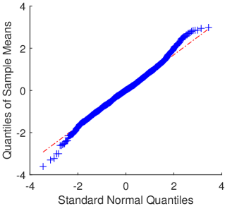
(a) True classes and scaling

(b) True classes, estimated scaling

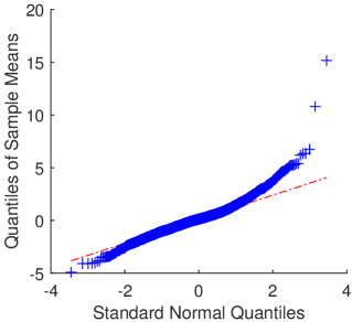
(c) Estimated classes and scaling

Figure 1: Q-Q plots of standardized sample means $\boldsymbol{\mathbf{y}}^{t}$ for $10$ runs of the simulated networks experiment under three levels of estimation. With LABEL:sub@fig:QQ128TrueTrue true classes and scaling factors, $\boldsymbol{\mathbf{y}}^{t}$ is close to the asymptotic Gaussian distribution predicted by Theorem 1. Even with LABEL:sub@fig:QQ128TrueEst estimated scaling factors, $\boldsymbol{\mathbf{y}}^{t}$ is still close to the asymptotic Gaussian distribution. When LABEL:sub@fig:QQ128EstEst class memberships are also estimated, $\boldsymbol{\mathbf{y}}^{t}$ is heavier tailed due to the errors in the estimated classes.

I begin by checking the validity of the asymptotic Gaussian distribution of the scaled sample means $\boldsymbol{\mathbf{y}}^{t}$. In this simulation experiment, the population means and standard deviations for $\boldsymbol{\mathbf{y}}^{t}$ are known and are used to standardize $\boldsymbol{\mathbf{y}}^{t}$. Q-Q plots for the standardized $\boldsymbol{\mathbf{y}}^{t}$ are shown in Figure 1. Figure 1a shows the distribution of $\boldsymbol{\mathbf{y}}^{t}$ when both the true classes and true scaling factors (calculated using the true states) are used. Notice that the empirical distribution is close to the asymptotic Gaussian distribution, with only slightly heavier tail. Experimentally I find that this deviation decreases as the block sizes increase, as one would expect from Theorem 1.

Figure 1b shows that the distribution of $\boldsymbol{\mathbf{y}}^{t}$ is roughly the same when using estimated scaling factors along with the true classes, which is an encouraging result and suggests that the EKF-based inference procedure would likely work well in the a priori block model setting. Figure 1c shows that the distribution of $\boldsymbol{\mathbf{y}}^{t}$ when using both estimated scaling factors and classes is significantly more heavy-tailed. Since this is not seen in Figure 1b, I conclude that it is due to errors in the class estimation, which causes the distribution of $\boldsymbol{\mathbf{y}}^{t}$ to deviate from the asymptotically Gaussian distribution when using true classes. The heavier tails suggest that perhaps a more robust filter, such as a filter that assumes Student-t distributed observations, may provide more accurate estimates in the a posteriori setting.

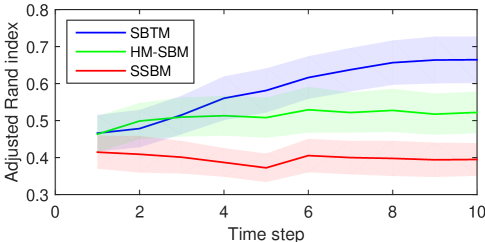
Figure 2: Adjusted Rand indices with $95\%$ confidence bands for the stochastic block transition model (SBTM), hidden Markov stochastic block model (HM-SBM), and static stochastic block model (SSBM) on $50$ runs of the simulated networks experiment.

Figure 2 shows a comparison of the class estimation accuracies, measured by the adjusted Rand indices (Hubert and Arabie, 1985), of three different inference algorithms: the EKF-based algorithm for the SBTM proposed in this paper, the EKF algorithm for the HM-SBM (Xu and Hero III, 2014), and a static SBM fit using spectral clustering on each snapshot. As one might expect, the static SBM approach does not improve as more time snapshots are provided. The poorer performance of the HM-SBM approach compared to the proposed SBTM approach is also not too surprising since the dynamics on the marginal block probabilities no longer follow a dynamic linear system as assumed by Xu and Hero III (2014). The SBTM approach is more accurate than the other two; however it still makes enough mistakes to cause the heavier-tailed distribution of $\boldsymbol{\mathbf{y}}^{t}$ as previously discussed.

6.2 Facebook Wall Posts

I now test the proposed SBTM inference algorithm on a real data set, namely a dynamic social network of Facebook wall posts (Viswanath et al., 2009). Similar to the analysis by Viswanath et al. (2009), I use $90$-day time steps from the start of the data trace in June 2006, with the final complete $90$-day interval ending in November 2008, resulting in $9$ total time steps. I filter out people who were active for less than $7$ of the $9$ times as well as those with in- or out-degree less than $30$, leaving $462$ remaining people (nodes).

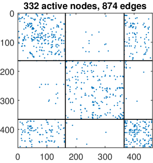
(a) $t=1$

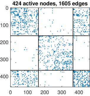
(b) $t=4$

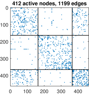
(c) $t=7$

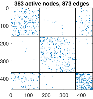
(d) $t=9$

Figure 3: Adjacency matrices at four different time steps constructed from Facebook wall posts. The estimated classes at the final time $t=9$ are overlaid onto the adjacency matrices.

I fit the SBTM to this dynamic network using Algorithm 1, beginning with a spectral clustering initialization at the first time step. From examination of the singular values of the first snapshot, I choose a fit with $k=3$ classes. Visualizations of the class structure overlaid onto the adjacency matrices at several time steps are shown in Figure 3. Notice that all of the classes are actually communities, with denser diagonal blocks compared to off-diagonal blocks. The initial snapshot contains only $332$ active nodes, so many new nodes enter the network over time. The networks are quite sparse, with the densest block having estimated marginal edge probability of about $0.08$. I find that the estimated probabilities of forming new edges is very low, less than $0.03$ over all time steps regardless of block. The probabilities of existing edges re-occurring show greater variation between blocks, ranging from about $0.18$ to $0.90$.

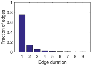
(a) Observed network

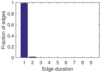
(b) HM-SBM simulated networks

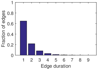
(c) SBTM simulated networks

Figure 4: Histograms of edge durations in LABEL:sub@fig:FacebookDurHistObs observed Facebook network, LABEL:sub@fig:FacebookDurHistHmSbm simulated networks from HM-SBM fit to observed network, and LABEL:sub@fig:FacebookDurHistSbtm simulated networks from SBTM fit to observed network. The HM-SBM cannot reproduce the observed edge durations, unlike the SBTM.

A histogram of the edge durations observed in the network is shown in Figure 4a. Notice that, despite the low densities of the blocks, more than $20\%$ of the edges appear over multiple time steps. I generate $10$ synthetic networks each from the HM-SBM and SBTM fits to the observed networks. The histogram of edge durations from synthetic networks generated from the HM-SBM is shown in Figure 4b. Due to the hidden Markov assumption, only the densities of the blocks are being replicated over time, and as such, the majority of edges are not repeated at the following time step. Compare this to the edge durations generated from the proposed SBTM, shown in Figure 4c. Notice that a significant fraction of edges are indeed repeated in these synthetic networks, much like in the observed networks. These edge durations cannot be replicated by the HM-SBM. Thus the proposed SBTM provides better fits to the sequence of observed adjacency matrices and allows it to better forecast future interactions.

Notice also that the edge durations from the synthetic networks are actually slightly longer than from the observed networks. This is an artifact that appears because not all nodes are active at all time steps in the observed networks, causing edge durations to be shortened in the observed networks. One could perhaps replicate this effect by adding a layer to the dynamic model simulating nodes entering and leaving the network over time, which would be an interesting direction for future work.

The proposed SBTM can also be extended to have edges depend directly on whether edges were present further back than just the previous time step. Such an approach would likely improve forecasting ability; however, it also increases the number of states that need to be estimated, which creates additional challenges that would make for interesting future work.

Acknowledgements

The author thanks Prof. Alan Mislove for providing access to the Facebook data analyzed in this paper.

References

- Billingsley (1995) P. Billingsley. Probability and measure. Wiley-Interscience, 3rd edition, 1995.
- Durante and Dunson (2014) D. Durante and D. B. Dunson. Nonparametric Bayes dynamic modelling of relational data. Biometrika, 101(4):883–898, 2014.
- Foulds et al. (2011) J. R. Foulds, C. DuBois, A. U. Asuncion, C. T. Butts, and P. Smyth. A dynamic relational infinite feature model for longitudinal social networks. In Proceedings of the 14th International Conference on Artificial Intelligence and Statistics, pages 287–295, 2011.
- Goldenberg et al. (2009) A. Goldenberg, A. X. Zheng, S. E. Fienberg, and E. M. Airoldi. A survey of statistical network models. Foundations and Trends in Machine Learning, 2(2):129–233, 2009.
- Guo et al. (2007) F. Guo, S. Hanneke, W. Fu, and E. P. Xing. Recovering temporally rewiring networks: A model-based approach. In Proceedings of the 24th International Conference on Machine Learning, pages 321–328, 2007.
- Heaukulani and Ghahramani (2013) C. Heaukulani and Z. Ghahramani. Dynamic probabilistic models for latent feature propagation in social networks. In Proceedings of the 30th International Conference on Machine Learning, pages 275–283, 2013.
- Ho et al. (2011) Q. Ho, L. Song, and E. P. Xing. Evolving cluster mixed-membership blockmodel for time-varying networks. In Proceedings of the 14th International Conference on Artificial Intelligence and Statistics, pages 342–350, 2011.
- Hoff (2011) P. D. Hoff. Hierarchical multilinear models for multiway data. Computational Statistics and Data Analysis, 55(1):530–543, 2011.
- Holland et al. (1983) P. W. Holland, K. B. Laskey, and S. Leinhardt. Stochastic blockmodels: First steps. Social Networks, 5(2):109–137, 1983.
- Hubert and Arabie (1985) L. Hubert and P. Arabie. Comparing partitions. Journal of Classification, 2(1):193–218, 1985.
- Ishiguro et al. (2010) K. Ishiguro, T. Iwata, N. Ueda, and J. B. Tenenbaum. Dynamic infinite relational model for time-varying relational data analysis. In Advances in Neural Information Processing Systems 23, pages 919–927, 2010.
- Kim and Leskovec (2013) M. Kim and J. Leskovec. Nonparametric multi-group membership model for dynamic networks. In Advances in Neural Information Processing Systems 25, pages 1385–1393, 2013.
- Lee and Priebe (2011) N. H. Lee and C. E. Priebe. A latent process model for time series of attributed random graphs. Statistical Inference for Stochastic Processes, 14(3):231–253, 2011.
- Nelson (2000) A. T. Nelson. Nonlinear estimation and modeling of noisy time-series by dual Kalman filtering methods. PhD thesis, Oregon Graduate Institute of Science and Technology, 2000.
- Sarkar and Moore (2005) P. Sarkar and A. W. Moore. Dynamic social network analysis using latent space models. ACM SIGKDD Explorations Newsletter, 7(2):31–40, 2005.
- Sarkar et al. (2007) P. Sarkar, S. M. Siddiq, and G. J. Gordon. A latent space approach to dynamic embedding of co-occurrence data. In Proceedings of the 11th International Conference on Artificial Intelligence and Statistics, pages 420–427, 2007.
- Sussman et al. (2012) D. L. Sussman, M. Tang, D. E. Fishkind, and C. E. Priebe. A consistent adjacency spectral embedding for stochastic blockmodel graphs. Journal of the American Statistical Association, 107(499):1119–1128, 2012.
- Viswanath et al. (2009) B. Viswanath, A. Mislove, M. Cha, and K. P. Gummadi. On the evolution of user interaction in Facebook. In Proceedings of the 2nd ACM Workshop on Online Social Networks, pages 37–42, 2009.
- Xing et al. (2010) E. P. Xing, W. Fu, and L. Song. A state-space mixed membership blockmodel for dynamic network tomography. The Annals of Applied Statistics, 4(2):535–566, 2010.
- Xu and Hero III (2014) K. S. Xu and A. O. Hero III. Dynamic stochastic blockmodels for time-evolving social networks. IEEE Journal of Selected Topics in Signal Processing, 8(4):552–562, 2014.
- Yang et al. (2011) T. Yang, Y. Chi, S. Zhu, Y. Gong, and R. Jin. Detecting communities and their evolutions in dynamic social networks—a Bayesian approach. Machine Learning, 82(2):157–189, 2011.