Newly-Discovered Planets Orbiting HD 5319, HD 11506, HD 75784 and HD 10442 from the N2K Consortium

Abstract

Initially designed to discover short-period planets, the N2K campaign has since evolved to discover new worlds at large separations from their host stars. Detecting such worlds will help determine the giant planet occurrence at semi-major axes beyond the ice line, where gas giants are thought to mostly form. Here we report four newly-discovered gas giant planets (with minimum masses ranging from 0.4 to 2.1 $M_{\rm Jup}$) orbiting stars monitored as part of the N2K program. Two of these planets orbit stars already known to host planets: HD 5319 and HD 11506. The remaining discoveries reside in previously-unknown planetary systems: HD 10442 and HD 75784. The refined orbital period of the inner planet orbiting HD 5319 is 641 days. The newly-discovered outer planet orbits in $886$ days. The large masses combined with the proximity to a 4:3 mean motion resonance make this system a challenge to explain with current formation and migration theories. HD 11506 has one confirmed planet, and here we confirm a second. The outer planet has an orbital period of $1627.5$ days, and the newly-discovered inner planet orbits in $223.6$ days. A planet has also been discovered orbiting HD 75784 with an orbital period of $341.7$ days. There is evidence for a longer period signal; however, several more years of observations are needed to put tight constraints on the Keplerian parameters for the outer planet. Lastly, an additional planet has been detected orbiting HD 10442 with a period of $1043$ days.

1. Introduction

Many details concerning planet formation and evolution have been gleaned from the ensemble of observed extrasolar planetary systems. An early example is the paradigm shift caused by the first few systems discovered, which contained gas giant planets orbiting well within the snow line (Mayor & Queloz 1995; Marcy & Butler 1996). This challenged the prevailing planet formation theory, in which planets form and remain several astronomical units (AU) from their parent stars (Lissauer 1993; Pollack et al. 1996). Planet formation theory quickly evolved to explain the newly-discovered systems in terms of migration (Lin et al. 1996).

As the number of discovered planetary systems accumulated, new connections between stellar parameters and the occurrence of planets became apparent. With only seven extrasolar planetary systems known at the time, Gonzalez (1997) noted a shared characteristic that four of the host stars had super-solar metallicities. As the number of known planetary systems grew, the connection between host star metallicity and giant planet occurrence became more pronounced. This culminated with Santos et al. (2004) measuring elemental abundances of 139 stars (98 known to host giant planets and 41 with no known companions), and Fischer & Valenti (2005) performing a thorough statistical analysis of 850 FGK-type stars, revealing the giant planet-metallicity correlation.

The more favorable detection rate for gas giant planets orbiting metal-rich stars combined with the exceptional scientific pay-off of transiting planets inspired a focused search for short-period gas giant planets orbiting metal-rich stars: the N2K (Next 2000 target stars) Doppler Survey (Fischer et al. 2005). Some particularly interesting transiting planets discovered as part of this program include HD 17156 b, a highly-eccentric transiting planet (Fischer et al. 2007; Barbieri et al. 2007; Schlaufman 2010; Lewis et al. 2011), and HD 149026 b, a surprisingly dense transiting hot-Jupiter (Sato et al. 2005; Fortney et al. 2005; Dodson-Robinson & Bodenheimer 2009; Anderson & Adams 2012). Doppler measurements of these systems can reveal valuable information concerning their migration history.

Table 1N2K Discoveries

Star ID	Period	$M_{P}\sin{i}$	Reference
	[d]	[$M_{\rm Jup}$]
HD 86081 b	2.14	1.50	Johnson et al. (2006)
HD 149026 b	2.88	0.36	Sato et al. (2005)
HD 88133 b	3.42	0.30	Fischer et al. (2005)
HD 149143 b	4.07	1.33	Fischer et al. (2006)
HD 125612 c	4.15	0.06	Fischer et al. (2007)
HD 109749 b	5.24	0.28	Fischer et al. (2006)
HIP 14810 b	6.67	3.87	Wright et al. (2007)
HD 179079 b	14.5	0.08	Valenti et al. (2009)
HD 33283 b	18.2	0.33	Johnson et al. (2006)
HD 17156 b	21.2	3.30	Fischer et al. (2007)
HD 224693 b	26.7	0.72	Johnson et al. (2006)
HD 163607 b	75.3	0.77	Giguere et al. (2012)
HD 231701 b	142	1.09	Fischer et al. (2007)
HIP 14810 c	148	1.28	Wright et al. (2007)
HD 154672 b	164	5.01	López-Morales et al. (2008)
HD 11506 c	223	0.40	this work
HD 205739 b	280	1.49	López-Morales et al. (2008)
HD 164509 b	282	0.48	Giguere et al. (2012)
HD 75784 b	342	1.15	this work
HD 75898 b	418	2.52	Robinson et al. (2007)
HD 16760 b	465	13.3	Sato et al. (2009)
HD 96167 b	499	0.69	Peek et al. (2009)
HD 125612 b	559	3.07	Fischer et al. (2007)
HD 5319 b	641	1.76	this work and Robinson et al. (2007)
HD 5319 c	886	1.15	this work
HD 16175 b	990	4.38	Peek et al. (2009)
HD 38801 b	696	10.0	Harakawa et al. (2010)
HIP 14810 d	951	0.58	Wright et al. (2009b)
HD 10442 b	1043	2.10	this work
HD 163607 c	1314	2.29	Giguere et al. (2012)
HD 11506 b	1617	4.80	this work and Fischer et al. (2007)
HD 73534 b	1770	1.07	Valenti et al. (2009)
HD 75784 c	5040	5.6	this work

Planets are thought to migrate either through planet-disk interactions via Type I and Type II migration (Goldreich & Tremaine 1980; Lin et al. 1996; Ida & Lin 2004), or through gravitational interactions. The latter mechanism includes interactions either with other planets in the system (Ford & Rasio 2008; Chatterjee et al. 2008; Wu & Lithwick 2011), or with other stars via the Kozai mechanism (Wu & Murray 2003; Fabrycky & Tremaine 2007). If planets migrate slowly through Type I or II migration, their orbital axes remain well-aligned with the rotational axes of their host stars. If planets migrate through gravitational interactions, their orbital axes are more likely to be misaligned relative to the rotational axes of their host stars (Chatterjee et al. 2008). By measuring the Rossiter-McLaughlin Effect, the spin-orbit alignment (obliquity) can be calculated for these hot Jupiter transiting systems (Winn et al. 2005, 2010), shedding light onto the dominant migration mechanism.

This hypothesis assumes that the protoplanetary disks from which planets are born are well-aligned with the rotational axes of the stars they surround. Based on the Solar System, this assumption appears valid (Lissauer 1993). However, this has been recently called into question in both single-star and multiple-star systems (Bate et al. 2010; Lai et al. 2011; Batygin 2012). Greaves et al. (2014) have examined 11 single-star systems with Herschel where the stellar inclination was known and the surrounding dust belts were spatially resolved. They found that all 11 disk-star spin angles were well-aligned, showing that misalignment mechanisms operate rarely in single star systems. Additionally, there are currently at least two observational programs exploring misalignment in binary systems: one is looking at the spin-orbit alignments in eclipsing binary star systems (Albrecht et al. 2013), while the other is searching for unbeknownst widely-separated massive companions in transiting hot Jupiter systems where obliquities have been measured (Knutson et al. 2013).

While most of the short-period gas giants have been detected, the mechanisms under which planets migrate can still be assessed through extended monitoring. Increasing the number of observations for each target star probes for lower mass and longer period planets. The mass detection limit is lowered because increasing the number of observations increases the signal-to-noise ratio. Additionally, more widely separated planets can be detected due to a longer observation time baseline. Building up a large population of these long period planets will be useful in determining the occurrence rate of planets at larger separations where they are thought to have formed. These statistically significant occurrence rates can then be used to test and refine population synthesis models that take both disk and gravitational migration mechanisms into account (Alibert et al. 2013; Ida et al. 2013). Lastly, building up a large sample of long time baseline observations will allow for comparison with other observing methods such as microlensing (Cassan et al. 2012) and direct imaging (Hartung et al. 2013; Beuzit et al. 2008). This paper presents the latest 4 planets discovered through the N2K consortium, bringing the total number of exoplanets discovered thus far through the N2K program to 32.

2. The N2K Program

The N2K target reservoir contains roughly 14,000 stars selected from the $Hipparcos$ Catalog that have $0.4<B-V<1.2$, distances closer than 110 parsecs, and $V<10.5$. Photometric estimates for the temperatures and metallicities of these stars were developed by Ammons et al. (2006). The reservoir star sample was then ranked according to these metallicity estimates. The N2K program had a very targeted strategy for rapid detection: a set of stars were observed for three or four (nearly) consecutive nights to search for short-period radial velocity variations consistent with orbiting hot Jupiters. Simulations showed that with this observing strategy 90% of exoplanets with $M_{P}\sin{i}$ $>0.5$ $M_{\rm Jup}$ and orbital periods shorter than 14 days would exhibit 20 m s^-1 scatter in the RV measurements (Fischer et al. 2005). Stars showing scatter greater than 10 m s^-1 were followed up with additional observations and stars with low rms scatter were retired to the database. The most obvious short period gas giant planets were detected first; however, monitoring continues on the N2K sample for longer period and multi-planet systems. To date about 560 stars have been observed at Keck as part of the N2K survey, and nearly three dozen planet detections (listed in Table 1) have been published from the project, with more emerging planet candidates.

3. Data Analysis

High resolution (R$\approx$55,000) spectroscopic observations of the stars discussed in this paper – HD 5319, HD 10442, HD 75784, and HD 11506 – were made using Keck HIRES (Vogt et al. 1994). Typical signal-to-noise ratios of our observations were about 150 per pixel. For each star, at least one high resolution observation was taken without the iodine (I₂) cell in the optical path. From these non-I₂ spectra, stellar parameters ($T_{\rm eff}$, [Fe/H], $\log g$ and $v\sin i$, and elemental abundances for Na, Si, Ti, Fe and Ni) were derived using the LTE spectral synthesis analysis software Spectroscopy Made Easy (SME) (Valenti & Piskunov 1996; Valenti & Fischer 2005). After generating an initial synthetic model, if parallax measurements were available, we iterated between the Y² isochrones (Demarque et al. 2004) and SME model as described by Valenti et al. (2009) until agreement in the surface gravity converged to 0.001 dex. The stellar mass, luminosity and ages that we present in the following sections were from the Y² isochrones (Demarque et al. 2004), where bolometric luminosity corrections were adopted from VandenBerg & Clem (2003).

The HIRES spectral format includes the Ca II lines, which are valuable because line core emission in the Ca II lines is a good indicator of chromospheric activity (Noyes et al. 1984). This is important for detecting planets via the radial velocity method since chromospheric activity is correlated with increased magnetic fields in stellar photospheres, which drive phenomena like the suppression of convection, stellar spots, and long term activity cycles (Saar & Donahue 1997; Saar & Fischer 2000; Santos et al. 2010; Lovis et al. 2011; Dumusque et al. 2011). All of these phenomena produce line profile variations that can be misinterpreted as Doppler shifts of the star. These sources of Doppler measurement errors are often combined into one term called stellar “jitter”. Isaacson & Fischer (2010) measured emission in the Ca II line cores to derive $S_{\rm HK}$ values and $\log{R^{\prime}_{HK}}$ (the ratio of emission in the core of the Ca II lines to the surrounding continuum). They have estimated astrophysical jitter measurements as a function of B V color, luminosity class, and excess $S_{\rm HK}$ values, and we have adopted those stellar jitter estimates for the stars in this paper.

Prior to taking Doppler observations, a high resolution (R$\approx$1,000,000), high signal-to-noise ratio ($\approx$1000) spectrum of an iodine cell was obtained with a Fourier Transform Spectrograph (FTS). This FTS scan was then used in determining Doppler shift measurements with a forward-modeling process (Butler et al. 1996). First, the intrinsic stellar spectrum (ISS) was obtained for each star by deconvolving a high resolution, high signal-to-noise non-I₂ spectrum to remove the spectral line spread function (SLSF), which is sometimes referred to as the point spread function. For all subsequent observations, the iodine cell was placed in the light path to imprint a dense ${\rm I_{2}}$ absorption spectrum on the stellar spectrum. The iodine lines were used to provide wavelength calibration and to model the SLSF for our observations. Finally, we multiplied the ISS and FTS ${\rm I_{2}}$ spectra and convolved the product with a SLSF sum of Gaussians model to match each program observation (Valenti et al. 1995). The modeling process was driven by a Levenberg-Marquardt algorithm, and the free parameters included the Doppler shift, the wavelength solution and the SLSF parameters.

The time series radial velocity data were then analyzed and fit with Keplerian models using Keplerian Fitting Made Easy (KFME) (Giguere et al. 2012). This graphical user interface was written in the Interactive Data Language (IDL) as a widget application. Multiple planets in each system can be fit either simultaneously or sequentially. KFME includes built in statistical analysis tools, such as periodogram false alarm probability (FAP) and Keplerian FAP tests (Wright et al. 2007; Johnson et al. 2007; Howard et al. 2009). Within KFME, orbital parameter confidence levels can be determined using a bootstrap Monte Carlo method (Press et al. 1992; Marcy et al. 2005).

A Bayesian approach was also taken to analyze the time series radial velocity measurements for each star. Each set of radial velocity measurements was fit with a Differential Evolution Markov Chain Monte Carlo algorithm. Additionally, for the multi-planet systems dynamical stability was taken into account through n-body integrations, where solutions with close-encounters were rejected (Johnson et al. 2011; Nelson et al. 2013).

Table 2Stellar Parameters

	HD 5319	HD 10442	HD 11506	HD 75784
Spectral type	K3 IV	K2 IV	G0 V	K3 IV
$V$	$8.05$	$7.84$	$7.51$	$7.84$
$M_{V}$	$2.76$		$3.94$	$3.15$
$B-V$	$0.99$	$0.93$	$0.61$	$0.99$
BC	$-0.30$	$-0.27$	$-0.04$	$-0.32$
Distance (pc)	$114$($11$)		$51.7$($1.6$)	$68.7$($6.2$)
$T_{\rm eff}$ (K)	$4958$($44$)	$5034$($44$)	$6055$($44$)	$4917$($44$)
$\log g$	$3.45$($0.06$)	$3.50$($0.06$)	$4.30$($0.06$)	$3.56$($0.06$)
${\rm[Fe/H]}$	$0.15$($0.03$)	$0.11$($0.03$)	$0.29$($0.03$)	$0.25$($0.03$)
$M_{\star}$ ($M_{\odot}$)	$1.51$($0.11$)	$1.56$($0.09$)	$1.24$($0.02$)	$1.41$($0.08$)
$R_{\star}$ ($R_{\odot}$)	$3.85$($0.40$)		$1.33$($0.05$)	$3.3$($0.3$)
$L_{\star}$ ($L_{\odot}$)	$8.1$($1.6$)		$2.13$($0.16$)	$5.7$($0.9$)
Age (Gyr)	$3.1$($0.6$)		$2.4$($0.6$)	$4.0$($0.7$)
log R’HK	$-5.28$	$-5.17$	$-4.98$	$-5.24$

4. HD 5319

4.1. Stellar Characteristics

Based on measurements from the original (ESA 1997) and the revised (van Leeuwen 2007) $Hipparcos$ Catalog HD 5319 (HIP 4297) is at a distance of $114$ $\pm$ $11$ pc. We adopted the Hipparcos V-band magnitude and color of V = $8.05$ and B V = $0.99$, applied a bolometric correction of $-0.30$  and calculated the absolute visual magnitude, $M_{V}=$$2.76$.

An iodine-free “template” spectrum of HD 5319 was analyzed by iterating SME models with Y² isochrones to derive the following stellar parameters: $T_{\rm eff}$ = $4958$ $\pm$ $44$ K, [Fe/H] = $0.15$ $\pm$ $0.03$ dex, and $\log g$ = $3.45$ $\pm$ $0.06$. The isochrone analysis also yields a stellar mass of $1.51$ $\pm$ 0.11 $M_{\odot}$, an age of $3.1$ $\pm$ $0.6$ Gyr, a stellar radius of $3.85$ $\pm$ $0.40$ R_☉, and a luminosity of $8.1$ $\pm$ $1.6$ L_☉.

SIMBAD and $Hipparcos$ have this star listed as a G5 subgiant; however, based on both our SME results and the $Hipparcos$ B-V measurement, this star most closely resembles a K3 subgiant. HD 5319 has low chromospheric activity with $\log{R^{\prime}_{HK}}=\$$-5.28$ and an estimated stellar jitter of $4.2$ m s^-1. The stellar properties of HD 5319 are summarized in Table 2.

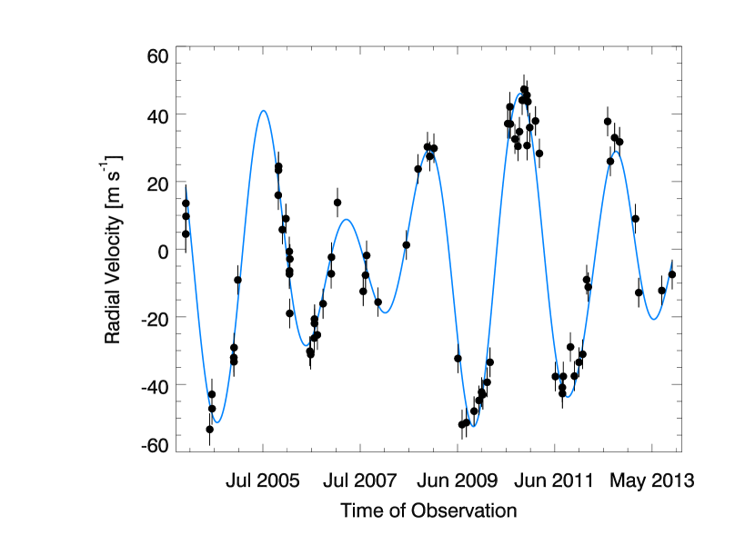
Figure 1.— Radial velocity measurements of HD 5319 with associated errors in black. The best-fit Keplerian model for the two-planet fit is superimposed in blue.

4.2. Doppler Observations & Orbital Solution

Based on the first 30 observations of HD 5319 over a time baseline of 3 years, Robinson et al. (2007) announced the discovery of HD 5319 b. Now with a total of $81$ observations and a time baseline spanning almost 10 years, an additional longer period planetary companion has been confidently detected. The best-fit double Keplerian model yields a slightly revised period for the inner planet of $641$ $\pm$ $2$ days with an eccentricity of $0.02$ $\pm$ $0.03$. Adopting a stellar mass of $1.51$ $M_{\odot}$, we derive a planet mass of $1.76$ $\pm$ $0.07$ $M_{\rm Jup}$. The newly-discovered outer planet has an orbital period of $886$ $\pm$ $8$ days, an eccentricity of $0.15$ $\pm$ $0.06$, and an inferred planet mass of $M_{P}\sin{i}$ = $1.15$ $\pm$ $0.08$ $M_{\rm Jup}$. The rms to the two-planet fit is $7.18$ m s^-1. Adding the jitter estimate of $4.2$ m s^-1 from Isaacson & Fischer (2010) in quadrature with the formal Doppler errors yields a $\chi_{\nu}^{2}$ of $2.64$. The 81 radial velocities of HD 5319 are shown in black in Figure 1.

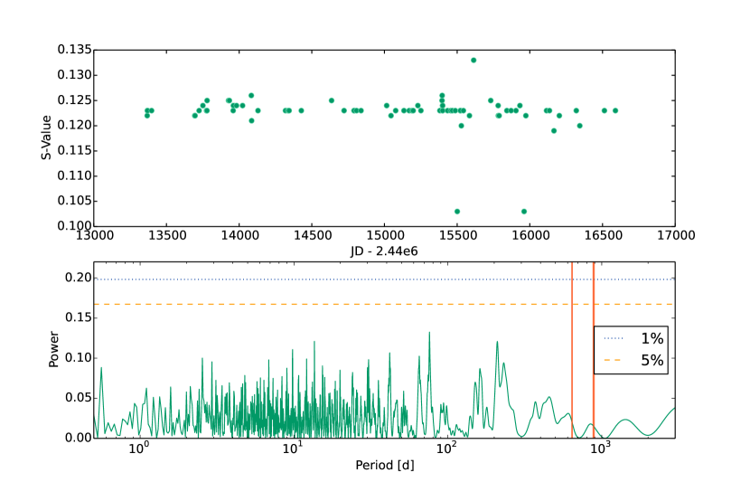
Figure 2.— S-Value measurements for each observation of HD 5319 are shown in the top panel and the corresponding GLS periodogram is shown in the bottom panel. Superimposed orange-dashed and blue-dotted horizontal lines indicate the 5% and 1% FAP levels, respectively. There is no significant power in the S-values at any period. The orbital periods of the two planets are shown as red vertical bars in the periodogram to highlight that the two planetary signals do not correspond with signals in the S-values.

One cause for concern is that one (or both) of these signals could be due to the magnetic cycle of the star masquerading as a long-period Keplerian signal. To address these concerns, we performed a generalized Lomb-Scargle periodogram analysis of the S_HK values (or simply S-values). We see no signs of magnetic variability in HD 5319. Figure 2 shows the S-value time series in the top panel and the associated GLS periodogram in the bottom panel. Superimposed in the bottom panel are horizontal lines indicating FAP levels of 5% (orange-dashed) and 1% (blue-dotted), which were determined by 1000 bootstrap resamplings of the data (Ivezić et al. 2013), and red vertical lines indicating the orbital periods of the planets. Since there is no peak in the periodogram above the 5% FAP line, there is no signal in the S-value measurements above 95% confidence.

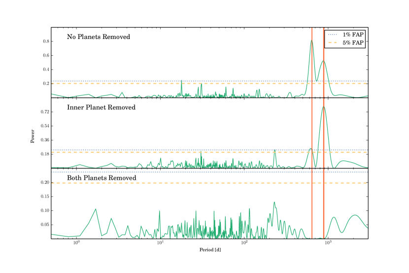
Figure 3.— (Top) Periodogram of RV measurements of HD 5319 demonstrating the strong periodic signal indicative of a planetary companion with a $\approx$640 day orbital period. The orange-dashed and blue-dotted horizontal lines show the 5% and 1% FAP thresholds, respectively. (Middle) Same as the top with the exception that the Keplerian model for the inner planet has been subtracted. The peak with the highest power corresponds to a period of $\approx$900 days, which motivated fitting for a second planet. (Bottom) Periodogram of the residuals of a two-planet model. The two red vertical lines show the best-fit orbital periods for the two planets. There is no significant power remaining and therefore fitting for additional planets is not warranted.

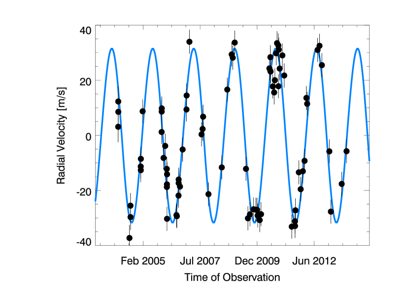
Figure 4.— RV measurements of HD 5319 with the superimposed Keplerian model for the inner planet, which has an orbital period of $641$ days. The Keplerian model for the outer planet has been subtracted.

Periodogram analysis of the radial velocity measurements shown in the top panel of Figure 3 reveals the dominant signal of the inner planet announced by Robinson et al. (2007) peaking at $\sim$625 days. Also shown in Figure 3 are the 5% and 1% FAP levels with orange dashed and blue dotted horizontal lines, respectively. Fitting the 625-day signal using KFME results in a $\chi_{\nu}^{2}$ of 9.3, motivating further inspection. Periodogram analysis of the single-planet fit residuals (middle panel of Figure 3) reveals an additional signal with a period of 909 days and a FAP $<$ 0.1%. Including an additional planet in the Keplerian model results in a significantly lower $\chi_{\nu}^{2}$ of $2.64$. Residual periodogram analysis to the two-planet solution (bottom panel of Figure 3) reveals no additional signals with significant power indicating any additional planets that may be orbiting HD 5319 are currently below our detection capabilities.

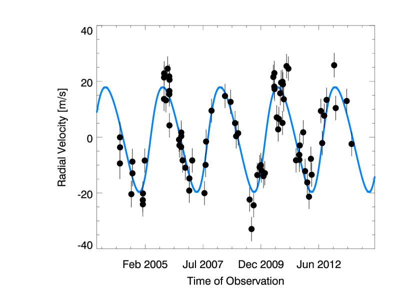
Figure 5.— RV measurements of HD 5319 after subtracting the best-fit model for the inner planet. The $886$ day Keplerian model for the outer planet is superimposed with a solid blue line.

The Keplerian models and radial velocity measurements for each of the two planets orbiting HD 5319 have been broken up into two figures to show the contributions and phase coverage of each planet. Figure 4 shows the residuals after subtracting the Keplerian model for the outer planet from the RV measurements. In other words, it is the radial velocity contribution from just the inner planet. The Keplerian model for just the inner planet is superimposed in blue. This shows both excellent phase coverage and that a Keplerian model accurately describes the data for the inner planet. Similar to Figure 4, Figure 5 shows the contributions and phase coverage of just the outer planet orbiting HD 5319 obtained by subtracting the Keplerian model of the inner planet. Again, there is excellent phase coverage and the Keplerian model for the outer planet accurately describes the data. The orbital parameters for the two planets detected orbiting HD 5319 are summarized in Table 3.

Table 3Orbital Parameters for the HD 5319 System

Parameter	HD 5319 b	HD 5319 c
P(d)	$641$ $\pm$ $2$	$886$ $\pm$ $8$
TP(JD)	$16288$ $\pm$ $790$	$13453$ $\pm$ $92$
e	$0.02$ $\pm$ $0.03$	$0.15$ $\pm$ $0.06$
$\omega$	$97$ $\pm$ $90$	$252$ $\pm$ $34$
K (m s-1)	$31.6$ $\pm$ $1.2$	$18.8$ $\pm$ $1.3$
a (au)	$1.6697$ $\pm$ $0.0036$	$2.071$ $\pm$ $0.013$
M $\sin{i}$ ($M_{\rm Jup}$)	$1.76$ $\pm$ $0.07$	$1.15$ $\pm$ $0.08$
N${}_{\textrm{obs}}$	$81$
Jitter (m s-1)	$4.2$
rms (m s-1)	$7.18$
$\chi_{\nu}^{2}$	$2.64$

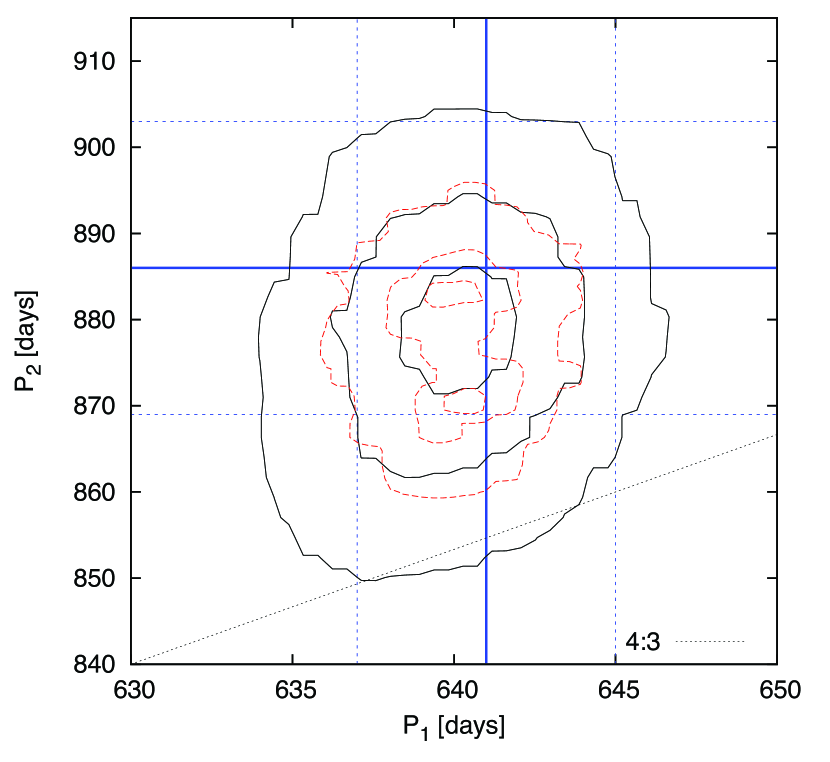
Figure 6.— Levenberg-Marquardt, Keplerian MCMC and N-body MCMC solutions for the orbital periods for the 2 planets orbiting HD 5319. The black lines are the 25%, 1-$\sigma$ and 2-$\sigma$ contours from a Keplerian MCMC analysis. The red contours are the same as the black, except dynamical stability has been taken into account through N-body simulations. The blue lines show the best-fit solution (solid) and 2-$\sigma$ uncertainties (dashed) using a Levenberg-Marquardt approach. To guide the eye, we have plotted the 4:3 period ratio as a diagonal dotted line.

To further increase confidence in our two-planet interpretation, we searched for a linear correlation between the S-values and RV measurements. The Pearson correlation coefficient ($\rho$) between the raw RV measurements and the S-values was -0.11. To quantify the lack of significance of this anti-correlation we created a distribution of $\rho$ by randomly sampling from the RVs with replacement (i.e., bootstrapping) 10,000 times. A p-value was then determined by counting the fraction of randomly sampled data sets that had a $|\rho|$ greater than our initial $\rho$ of the unscrambled data set. In this case our p-value was 0.33, which implies our measured $\rho$ does not differ significantly from the null hypothesis of $\rho$=0. We performed this same test with the residual velocity measurements: after subtracting the dominant (previously-published inner planet) 641-day signal we calculated a $\rho$ of -0.17 with a corresponding p-value of 0.16, again showing no significant linear correlation between the two parameters. Subtracting the Keplerian model of the outer planet and repeating this analysis resulted in a $\rho$ of 0 with a p-value of 1. Similarly, the result for the residuals to the fit for both planets was $\rho$=-0.10 with a p-value of 0.41. All of these tests were consistent with the null hypothesis, meaning there’s no correlation between the two parameters and reaffirming our two-planet interpretation.

As described at the end of §3, in addition to fitting the RV measurements with a Levenberg-Marquardt Least Squares Minimization scheme with KFME, a Bayesian approach was taken to analyze the data using the RUN DMC algorithm (Nelson et al. 2013). First, the radial velocity measurements were fitted with a double-Keplerian model using DEMCMC without taking dynamical stability into account. The resulting distribution of periods for the inner and outer planets are shown in black in Figure 6 with 25%, 1-$\sigma$ and 2-$\sigma$ confidence level contours. The blue solid lines are the best-fit solutions from KFME discussed earlier with the 2-$\sigma$ confidence levels shown as blue dashed lines. DEMCMC analysis produces a median solution that is consistent with the KFME result. The median periods from Keplerian MCMC analysis for the inner and outer planets with 1-$\sigma$ confidence levels are $640.1^{+2.4}_{-2.5}$ and $878^{+10}_{-11}$ days, respectively. The inferred minimum masses for the inner and outer planets are $1.68\pm 0.07$ and $1.03\pm 0.09$ $M_{\rm Jup}$, respectively.

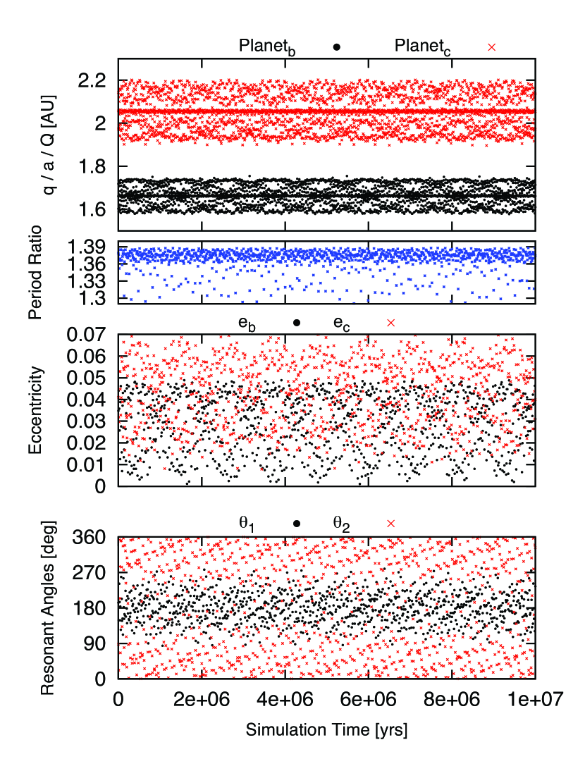
Figure 7.— One of the long-term dynamical evolution simulations where the HD 5319 system was stable over the entire $10^{7}$ yr integration period. Shown are the orbital semi-major axes ($a_{b}\,\&\,a_{c}$), period ratio, eccentricities ($e_{b}\,\&\,e_{c}$), and resonant angles ($\theta_{1}$ and $\theta_{2}$) as functions of time for the two planets orbiting HD 5319. We see that the system stably librates within the 4:3 resonance.

When a 100-year dynamical stability constraint is included with the RUN DMC algorithm, the majority of solutions are concentrated into the same region of parameter space as the Keplerian MCMC and KFME results, with median values for the orbital periods of the inner and outer planets of $640.1\pm 1.2$ and $878^{+6}_{-9}$ days, respectively. The only significant difference between the Keplerian MCMC and RUN DMC solutions is that when the 100-year dynamical stability is enforced the orbital period uncertainty decreases. These RUN DMC results are superimposed in red long-dashed contours showing the 25%, 1-$\sigma$ and 2-$\sigma$ levels in Figure 6.

Simulations testing the dynamical stability over longer periods (10⁷ years) were carried out using MERCURY (Chambers 1999). Most of the realizations were unstable; however, several remained stable over the duration of the simulations. Of the realizations that were stable, all of them exhibited libration. While all three fitting methods resulted in best-fit period ratios that were slightly higher than 4:3, the best-fit solution only reflects our instantaneous “snapshot” of the system. Since all the long-term simulations that were stable exhibited libration, the long-term averaged orbital period ratio may be 4:3, which would put this system in the 4:3 mean motion resonance and not just close to it. In Figure 7 we provide an example of one of the stable solutions which occupy the 4:3 resonance, illustrating the oscillations in orbital elements as a function of time, as well as the evidence for libration in the resonant angles, $\theta_{1}$ and $\theta_{2}$. The resonant angles are defined as

$$\theta_{1}=4\left(\lambda_{2}-\varpi_{2}\right)-3\left(\lambda_{1}-\varpi_{1}\right)+3\left(\varpi_{2}-\varpi_{1}\right)$$ (1)

$$\theta_{2}=4\left(\lambda_{2}-\varpi_{2}\right)-3\left(\lambda_{1}-\varpi_{1}\right)+4\left(\varpi_{2}-\varpi_{1}\right)$$ (2)

where $\lambda_{i}$ and $\varpi_{i}$ are the mean longitude and longitude of periapse of the $i^{th}$ planet, respectively. This demonstrates that this system is stably librating within the 4:3 resonance. We note that the planetary eccentricities are highly oscillatory, with $e_{b}$ in this example frequently returning to an approximately circular ($e_{b}=0$) state.

Table 4RV Measurements of HD 5319

JD	RV	$\sigma_{RV}$	$S_{HK}$
-2440000	(m s-1)	(m s-1)
13014.7556	4.50	3.70
13015.7606	13.58	3.61
13016.7651	9.72	2.99
13191.1101	-53.30	2.22
13207.0754	-42.94	1.90
13208.0656	-47.18	2.12
13367.7078	-32.05	1.13	0.122
13368.7160	-33.30	1.22	0.123
13369.7253	-29.11	1.03	0.123
13397.7194	-9.11	1.00	0.123
13694.7659	15.97	1.02	0.122
13695.7711	23.36	0.98	0.122
13696.7462	24.52	1.00	0.122
13724.7791	5.79	0.91	0.123
13750.7363	9.04	1.28	0.124
13775.7200	-0.69	1.24	0.123
13776.7061	-7.33	1.19	0.123
13777.7208	-6.42	1.26	0.123
13778.7168	-19.00	1.20	0.123
13779.7412	-2.90	1.17	0.125
13927.0485	-30.18	1.22	0.125
13933.0449	-31.17	1.24	0.125
13959.0917	-26.29	1.27	0.123
13961.0367	-21.96	1.01	0.124
13961.0402	-20.66	1.00	0.124
13981.9060	-25.36	1.18	0.124
14023.7760	-16.13	1.36	0.124
14083.8337	-7.27	1.13	0.126
14085.9027	-2.36	1.22	0.121
14129.7746	13.80	1.08	0.123
14319.0740	-12.47	0.98	0.123
14336.0524	-7.68	1.01	0.123
14343.9381	-1.85	1.06	0.123
14427.9088	-15.65	0.98	0.123
14636.0956	1.25	1.12	0.125
14721.9810	23.72	1.20	0.123
14790.8874	30.29	1.28	0.123
14807.8193	27.46	1.13	0.123
14838.7959	29.85	1.08	0.123
15015.1236	-32.33	1.01	0.124
15045.0752	-51.89	1.23	0.122
15077.0750	-51.30	1.07	0.123
15133.9738	-47.91	1.15	0.123
15169.8628	-44.74	1.14	0.123
15188.7784	-42.27	1.17	0.123
15197.7498	-43.02	1.22	0.123
15229.7113	-39.36	1.14	0.124
15250.7109	-33.44	1.11	0.123
15381.1261	37.15	1.24	0.123
15396.1025	37.10	1.21	0.125
15397.0565	42.13	1.09	0.126
15400.0755	37.05	1.09	0.124
15434.0867	32.58	1.10	0.123
15455.9742	30.44	1.10	0.123
15467.0374	34.77	1.05	0.123
15487.0331	44.07	1.08	0.123
15500.8621	47.28	1.19	0.103
15521.8665	45.55	1.10	0.123
15522.8818	30.67	1.00	0.123
15528.8672	43.64	1.11	0.120
15542.8488	35.99	1.04	0.123
15584.7044	37.93	1.04	0.122
15613.7048	28.33	1.15	0.133
15731.1069	-37.67	1.12	0.125
15782.1153	-40.90	1.04	0.124
15783.1368	-42.71	1.14	0.122
15789.1394	-37.63	1.10	0.122
15841.9586	-28.92	1.13	0.123
15871.0018	-37.54	1.35	0.123
15904.7652	-33.46	1.28	0.123
15931.7529	-31.07	1.15	0.124
15960.7076	-9.01	1.14	0.103
15972.7134	-11.19	1.03	0.122
16115.1335	37.79	1.17	0.123
16135.1396	26.00	1.13	0.123
16166.1509	33.00	1.22	0.119
16202.9785	31.74	1.19	0.122
16319.7103	9.01	1.17	0.123
16343.7140	-12.85	1.16	0.120
16513.1415	-12.23	1.23	0.123
16588.9789	-7.49	1.22	0.123

There have been several systems near or in 4:3 mean motion resonances discovered by the Kepler Mission (Borucki et al. 2011; Lissauer et al. 2011; Batalha et al. 2013) and one other system (HD 200964) discovered by the radial velocity method (Johnson et al. 2011). The HD 200694 and HD 5319 systems are qualitatively different than the Kepler systems, in that the orbiting planets in these RV-detected systems have much longer orbital periods and are much more massive. A recent study by Rein et al. (2012) has tested a variety of formation and migration mechanisms attempting to recreate the observed distribution of planets in or near the 4:3 resonance. They found that while they could recreate the low mass Kepler systems, they could not reproduce gas giants in a 4:3 resonance. They tried several mechanisms for forming such a system: convergent migration, scattering and simultaneous damping, and in situ formation. All simulations either failed to create a system near a 4:3 resonance or required highly tuned initial conditions that produced 1:1 resonances three times more frequently, none of which have been observed. Although only two massive systems are known to be near the 4:3 resonance, Rein et al. (2012) conclude that the observed fraction of such systems is too high to explain with traditional formation mechanisms. They suggest two additional mechanisms that have not yet been investigated: resonant chain breaking and chaotic migration. However, the exact mechanism behind the formation of the HD 200964 and HD 5319 planetary systems is still a puzzle to be solved.

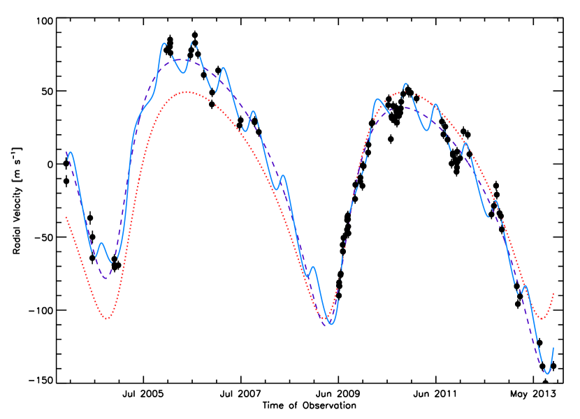
Figure 8.— Radial velocity measurements for HD 11506 (black). Superimposed are the theoretical models for one planet with no linear trend (red dotted), one planet with a linear trend (purple dashed), and two planets with a linear trend (blue solid).

5. HD 11506

5.1. Stellar Characteristics

HD 11506 (HIP 8770) is an early G dwarf star observed as part of the original N2K survey. The trigonometric parallax listed in the $Hipparcos$ catalog is 19.34  $\pm$ 0.58 mas, which corresponds to a distance 51.7  $\pm$ 0.6 pc. Combined with the Johnson V magnitude of $7.51$ also listed in the $Hipparcos$ catalog, we calculate an absolute visual magnitude of $3.94$. Iteration between SME and the $Y^{2}$ isochrones as described in §3 results in a best-fit metallicity of $0.29$ $\pm$ $0.03$; a surface gravity of $4.30$ $\pm$ $0.06$; and an effective temperature of $6055$ $\pm$ $44$ K. From iteration with the isochrones the stellar mass converges to $1.24$ $\pm$ $0.02$ $M_{\odot}$ with a stellar radius of $1.33$ $\pm$ $0.05$ $R_{\odot}$, a stellar luminosity of $2.13$ $\pm$ $0.16$ $L_{\odot}$, and an age of $2.4$ $\pm$ $0.6$ Gyr. The stellar parameters for HD 11506 are summarized in Table 2.

5.2. Doppler Observations & Orbital Solution

With 3.5 years of data accumulated, Fischer et al. (2007) announced the discovery of a planet orbiting HD 11506 with a period of 1405 days. They noted several remaining peaks in a periodogram of the residuals, including a peak at 170 days; however, they cautioned that more data were required to evaluate the second signal. Tuomi & Kotiranta (2009) carried out an extensive Bayesian analysis claiming that the second planet did indeed exist with an orbital period of 170.5${}^{+3.3}_{-6.2}$ days. However, their Bayesian analysis is roughly 48 $\sigma$ from the period we obtain with our extended data set.

Since the initial discovery paper by Fischer et al. (2007), HD 11506 has been observed an additional 87 times over the past 6 years. After subtracting the best-fit $\sim$1600-day Keplerian model (represented by a red-dotted line in Figure 8) from the RV measurements, the extended data set shows a clear long-period signal that is the dominant power in the periodogram of the residuals. This is shown in the second panel from the top in Figure 9. The period of this long-period signal is much longer than the time baseline of our observations, and it can be well-approximated as a linear trend. Incorporating this linear term (the purple-dashed line in Figure 8) reduced the $\chi_{\nu}^{2}$ from 36 for the single-planet fit to 9 for the single-planet + linear trend fit. Periodogram analysis of the residuals of the single-planet + linear trend model reveals the presence of an additional companion with a 223 day period, which is shown in the second panel from the bottom in Figure 9. The best-fit two-planet + linear trend solution, which has a $\chi_{\nu}^{2}$ of 2.94 and an rms of 5.8 is superimposed in solid blue in Figure 8. Since there is no significant power remaining in the residuals, fitting for additional planets is not warranted.

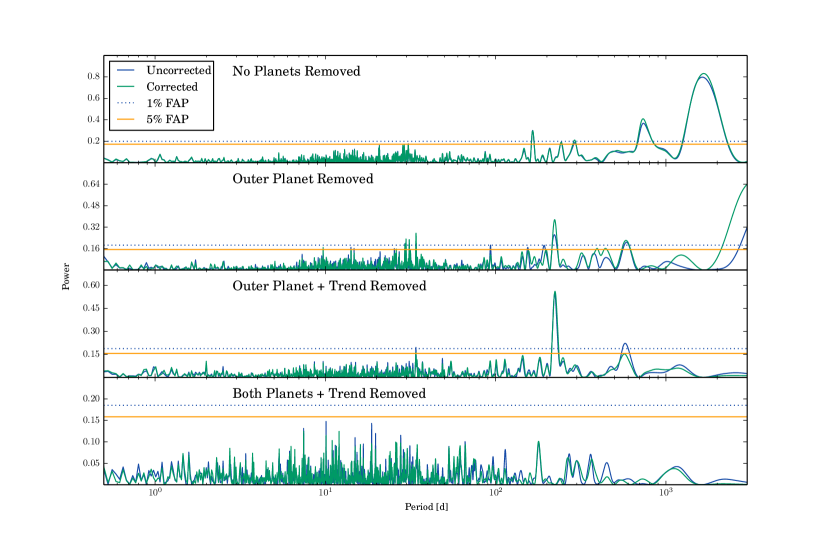
Figure 9.— Periodograms of the RV measurements of HD 11506 and the residuals after subtracting Keplerian and linear models. The green curve shows the power in the magnetic-signal-corrected time series and the blue curve shows the power in the uncorrected time series.

Similar to tests performed on the HD 5319 observations, we searched for signs of magnetic activity contributing to the RV measurements. Figure 10 shows the S-value time series (top panel) and the GLS periodogram of the S-values (bottom panel); the orbital periods of the two planets are superimposed in the bottom panel as red vertical lines. This shows that there is no period with $>$ 95% confidence at any power, and there are no peaks corresponding to the periods of the planets. Furthermore, periodogram power does not significantly increase towards longer periods, indicating the linear trend is not due to magnetic activity either.

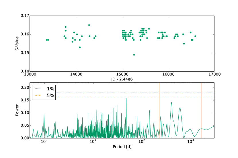
Figure 10.— Same as Figure 2, but for S-values of HD 11506 observations. Here it can be seen that there is no significant power due to magnetic activity at either of the planetary signals.

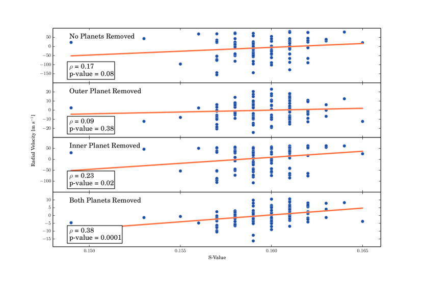
Figure 11.— RV Measurements and residuals for HD 11506 as a function of S-value. The top panel shows the raw RV measurements with no planetary Keplerian models subtracted, the middle two panels show the residuals after subtracting each best-fit keplerian model, and the bottom panel shows the residuals after subtracting both Keplerian models and a linear term from the RV data. There is no statistically significant correlation between the velocities and S-values when both planetary signals are present, but subtracting the planetary signals reveals a linear correlation between the residuals and the S-value measurements.

We also looked for correlations between the residual velocity measurements and the S-values as we did with HD 5319. The top panel of Figure 11 shows the RV measurements as a function of S-value for the raw velocity set. As described in §4.2, we calculated the Pearson correlation coefficient, $\rho$, and its associated p-value for these two parameters, which were 0.17 and 0.08, respectively. This indicates that there is no significant correlation between the “raw” velocities and the S-values. We then repeated the analysis after subtracting the Keplerian model of the outer planet from the velocity measurements; the results are shown in the second panel from the top in Figure 11. Again, there is no statistically significant linear correlation between the two parameters. Removing the model for the inner planet without removing the linear trend resulted in $\rho$ = 0.19 with a p-value of 0.05. To check the impact of this marginally significant linear correlation on our two-planet + linear trend interpretation we subtracted the linear model that best-fit the RV-S-value data from the velocity measurements and repeated the Keplerian modeling. This resulted in similar orbital parameters between the magnetic-signal-corrected and non-magnetic-signal-corrected RV measurements, but with an increase in rms. We then subtracted the Keplerian model of the inner planet and linear trend from the velocities and performed the same test on the residuals. Interestingly, a significant correlation between the two parameters emerged (second panel from the bottom).

Table 5Orbital Parameters for the HD 11506 System

Parameter	HD 11506 b	HD 11506 c
P(d)	$1627.5$ $\pm$ $5.9$	$223.6$ $\pm$ $0.6$
TP(JD)	$16637.2$ $\pm$ $7.6$	$14127$ $\pm$$9$
e	$0.37$ $\pm$ $0.01$	$0.24$ $\pm$ $0.05$
$\omega$	$218.9$ $\pm$ $1.6$	$272$ $\pm$ $15$
K (m s-1)	$78.4$ $\pm$ $1.2$	$12.5$ $\pm$ $0.7$
a (au)	$2.708$ $\pm$ $0.007$	$0.721$ $\pm$ $0.001$
M $\sin{i}$ ($M_{\rm Jup}$)	$4.21$ $\pm$ $0.07$	$0.36$ $\pm$ $0.02$
dv/dt (m s-1 yr-1)	$-7.19$ $\pm$ $0.26$
N${}_{\textrm{obs}}$	$107$
Jitter (m s-1)	$2.8$
rms (m s-1)	$4.80$
$\chi_{\nu}^{2}$	$2.20$

Lastly, we subtracted the full two-planet + linear trend model from the velocities and saw a very significant linear correlation between the two parameters ($\rho$ = 0.38, p-value = 0.0001), which can be seen in the bottom panel of Figure 11. Subtracting the best-fit linear model between these residual RV measurements and S-values from the original RV measurements and repeating the Keplerian analysis resulted in similar orbital parameters; however, after correcting for the magnetic signal the peaks in the periodograms were slightly higher at the periods corresponding to the planetary signals. We were interested to see if subtracting this magnetic signal and refitting would reveal additional planets in the system that were previously below the stellar noise level; however, power in the highest peaks in the residual periodogram decreased after correcting for the magnetic signal and no new signals emerged.

This Keplerian signal enhancement and noise reduction can be seen in Figure 9, where the uncorrected periodogram power is shown in blue and the magnetic-signal-corrected power is shown in green. Overall, subtracting the magnetic signal reduced the rms by 1.0 m s^-1(21%) relative to the uncorrected result. The final refined best-fit solution for the outer planet has an orbital period of $1627.5$ $\pm$ $5.9$ days, an eccentricity of $0.37$ $\pm$ $0.01$, and a radial velocity semi-amplitude of $78.4$ $\pm$ $1.2$ m s^-1. Based on these parameters the calculated semi-major axis is $2.708$ $\pm$ $0.007$ AU and the planet has a minimum mass of $4.21$ $\pm$ $0.07$ $M_{\rm Jup}$. The inner planet has a best-fit solution with an orbital period of $223.6$ $\pm$ $0.6$ days, an eccentricity of $0.24$ $\pm$ $0.05$, and a semi-amplitude of $12.5$ $\pm$ $0.7$ m s^-1. This corresponds to a semi-major axis of $0.721$ $\pm$ $0.001$ AU and a minimum mass of $0.36$ $\pm$ $0.02$ $M_{\rm Jup}$. These orbital parameters are summarized in Table 5 .

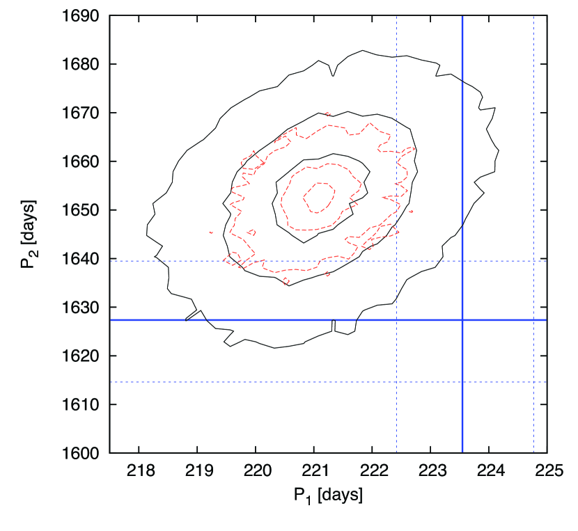
Figure 12.— Levenberg-Marquardt, Keplerian MCMC and N-body MCMC solutions for the orbital periods for the 2 planets orbiting HD 11506. The black lines are the 25%, 1-$\sigma$ and 2-$\sigma$ contours from a Keplerian MCMC analysis. The red contours are the same as the black with the exception that dynamical stability has been taken into account through N-body simulations. The blue lines show the best-fit solution (solid) and 2-$\sigma$ uncertainties (dashed) using the KFME Levenberg-Marquardt approach.

The Keplerian DEMCMC analysis shown in black in Figure 12 resulted in orbital periods for the inner and outer planets of $221.1\pm 1.1$ and $1653^{+11}_{-12}$ days, and minimum masses of $0.50\pm 0.06$ and $5.5\pm 0.2$ $M_{\rm Jup}$, respectively. Taking into account n-body interactions over short timescales, the n-body RUN DMC analysis resulted in consistent results with orbital periods of $221.1\pm 0.4$ and $1653\pm 4$ days, and minimum masses of $0.48^{0.03}_{-0.04}$ and $5.5\pm 0.1$ for the inner and outer planets, respectively. These are superimposed in Figure 12 in red along with the KFME results, which are in blue. The resulting period distributions from the DEMCMC and KFME analysis do not lie on top of each other, but there is considerable overlap in the 2-$\sigma$ wings of the distributions. There are a few possible explanations for the separation in the orbital solutions for the two models: the DEMCMC result is the median of the period distributions whereas the KFME solution is the best-fit, the difference in priors in each model plays a role, and the noise is assumed to be normally-distributed in the KFME analysis when it is most likely not exactly Gaussian.

Table 6RV Measurements of HD 11506

JD	RV	$\sigma_{RV}$	$S_{HK}$
-2440000	(m s-1)	(m s-1)
13014.7350	0.29	2.99
13015.7389	0.39	2.99
13016.7409	-11.77	2.99
13191.1220	-36.93	3.59
13207.1012	-64.34	3.14
13208.0840	-49.96	3.32
13368.8378	-65.01	1.70	0.157
13369.7590	-69.06	1.48	0.157
13370.7324	-70.80	1.65	0.157
13397.7301	-69.26	1.24	0.157
13750.7381	77.84	1.76	0.159
13775.7285	80.20	1.83	0.158
13776.7044	82.52	1.67	0.162
13777.7253	85.05	1.88	0.164
13778.7186	82.70	2.03	0.162
13779.7474	75.99	1.82	0.158
13926.1274	74.32	1.70	0.156
13933.0906	77.90	1.76	0.158
13959.1394	88.17	1.26	0.161
13961.1242	82.82	1.55	0.161
13981.9826	75.16	1.67	0.157
14023.9744	60.88	2.10	0.160
14083.8433	40.80	1.46	0.157
14085.9211	48.89	1.47	0.153
14129.7433	64.00	1.48	0.159
14286.1184	26.39	2.00	0.165
14295.0948	29.94	1.47	0.159
14396.8462	28.57	1.41	0.158
14397.9753	29.55	1.50	0.158
14427.9127	21.88	1.50	0.159
15015.1201	-90.04	1.62	0.159
15016.1145	-83.23	1.50	0.160
15017.1212	-81.06	1.53	0.161
15019.1232	-83.56	1.58	0.162
15027.1128	-75.93	1.46	0.159
15029.1124	-75.08	1.54	0.158
15043.1284	-55.30	1.55	0.160
15044.1334	-59.71	1.69	0.162
15045.1092	-59.90	1.58	0.161
15049.1053	-50.52	1.56	0.159
15074.1001	-47.75	1.55	0.157
15075.1049	-44.87	1.58	0.158
15076.0998	-38.41	1.67	0.158
15077.0913	-37.04	1.50	0.159
15078.0946	-36.01	1.50	0.161
15081.1111	-35.22	1.59	0.161
15082.0962	-37.89	1.57	0.160
15083.1074	-42.78	1.48	0.159
15085.0652	-47.45	1.75	0.157
15133.9969	-23.94	1.58	0.159
15135.9215	-14.21	1.59	0.160
15171.8999	-12.04	1.72	0.159
15172.8826	-9.32	1.65	0.161
15187.7268	-14.97	1.64	0.160
15189.8075	-1.12	1.56	0.161
15196.7897	-1.44	1.49	0.162
15229.7192	7.82	1.58	0.160
15231.7230	13.15	1.63	0.158
15255.7125	27.73	1.56	0.157
15260.7136	28.13	1.76	0.149
15377.1272	40.29	1.53	0.161
15381.1188	44.36	1.52	0.161
15396.1222	16.99	1.61	0.159
15401.0718	32.53	1.53	0.157
15403.1233	31.33	1.38	0.161
15405.0935	32.10	1.54	0.159
15411.1124	31.23	1.57	0.161
15413.0789	39.74	1.57	0.162
15426.0844	29.64	1.60	0.162
15435.0957	32.51	1.57	0.161
15436.0942	38.45	1.55	0.162
15437.1286	35.85	1.58	0.163
15439.1314	33.75	1.40	0.160
15441.1157	28.28	1.56	0.159
15455.9780	32.93	1.56	0.161
15465.0604	35.01	1.61	0.160
15469.0649	38.09	1.51	0.162
15471.9672	42.54	1.64	0.163
15487.0061	47.90	1.56	0.160
15521.8824	50.90	1.65	0.162
15528.8094	48.84	1.80	0.161
15542.9508	48.69	1.65	0.158
15584.7831	44.77	1.56	0.163
15771.0854	29.00	1.54	0.158
15782.1102	20.24	1.50	0.158
15795.1323	25.54	1.63	0.161
15812.1130	16.63	1.66	0.158
15842.0209	0.25	1.81	0.161
15850.9531	7.24	1.54	0.161
15852.0283	6.02	1.60	0.161
15870.9983	2.92	1.78	0.158
15877.9871	-5.31	1.64	0.159
15879.9690	0.77	1.56	0.160
15880.8704	-2.41	1.60	0.161
15881.8258	8.39	1.55	0.161
15903.7783	3.90	1.57	0.159
15928.8013	22.31	1.96	0.161
15960.7459	19.97	1.46	0.159
15972.7083	6.70	1.52	0.159
16134.1399	-34.52	1.60	0.158
16152.1129	-28.66	1.55	0.159
16168.0626	-14.84	1.72	0.160
16173.1109	-20.99	1.58	0.160
16193.0920	-33.64	1.79	0.160
16202.9956	-35.62	1.88	0.159
16210.0096	-44.80	1.66	0.159
16319.6985	-83.61	1.56	0.160
16327.7120	-95.80	1.54	0.160
16343.7092	-90.62	1.66	0.155
16487.1313	-122.30	1.60	0.161
16508.1360	-138.37	1.62	0.157
16530.0644	-149.89	1.58	0.157
16588.9923	-138.22	2.00	0.159

6. HD 75784

6.1. Stellar Characteristics

The $Hipparcos$ catalog lists a parallax of $11.54$  $\pm$ $0.83$ mas for HD 75784 (HIP 43569), which corresponds to a distance of $68.7$ $\pm$ $6.2$ pc. Spectral synthesis modeling with SME yields $T_{\rm eff}$ = $4917$ $\pm$ $44$ K, [Fe/H]= $0.25$ $\pm$ $0.03$ dex and $\log g$ = $3.56$ $\pm$ $0.06$. Iteration with the $Y^{2}$ isochrones yields a stellar mass of M_⋆= $1.41$ $\pm$ $0.08$ $M_{\odot}$, a stellar luminosity of L_⋆= $5.7$ $\pm$ $0.9$ $L_{\odot}$, a stellar radius of R_⋆= $3.3$ $\pm$ $0.3$ $R_{\odot}$, and an age of $4.0$ $\pm$ $0.7$ Gyr. The measured $\log g$ in combination with $T_{\rm eff}$ suggests a spectral type and luminosity class most consistent with a K3 subgiant (Johnson 1966; Gray 2008). While most of the individual elemental abundances were normal, it is worth noting the low [Si/Fe] abundance of -0.16 $\pm$ 0.05. This low Si abundance is at odds with the result of Brugamyer et al. (2011), where they found planet hosts to be enhanced in Si relative to Fe. The stellar parameters for HD 75784 are summarized in Table 2.

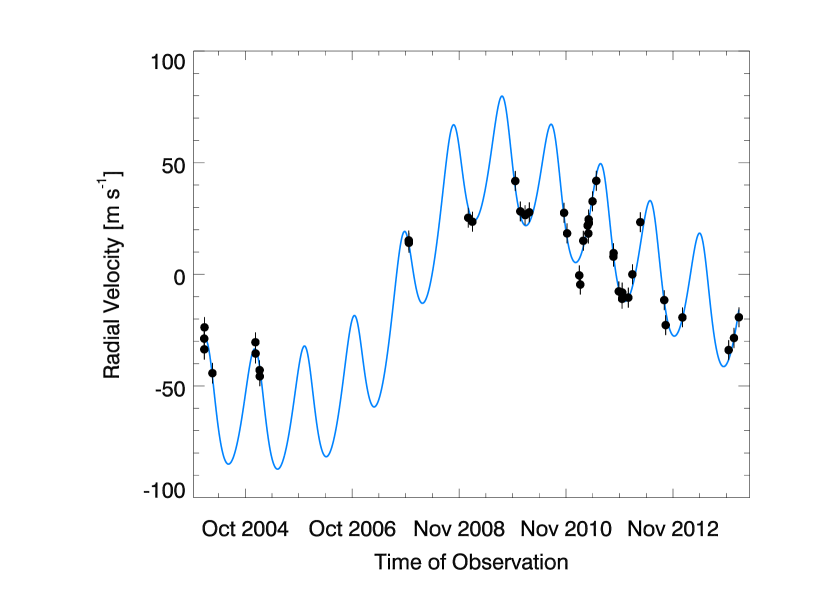
Figure 13.— Radial velocity measurements and associated uncertainties for HD 75784 are shown in black with the double Keplerian model for the two planets superimposed with a solid blue line.

6.2. Doppler Observations & Orbital Solution

Keck HIRES observations of HD 75784 date back to January of 2004, giving a time baseline of ten years for this star. The dominant signal, with an orbital period of $5040$ days and eccentricity of $0.36$, is significantly longer than our time baseline leading to a poorly-constrained solution using both frequentist and Bayesian approaches. We continue to monitor HD 75784 to refine the orbital solution for this long-period planet; however, with the current set of RV measurements we are able place tight constraints on an additional companion orbiting HD 75784.

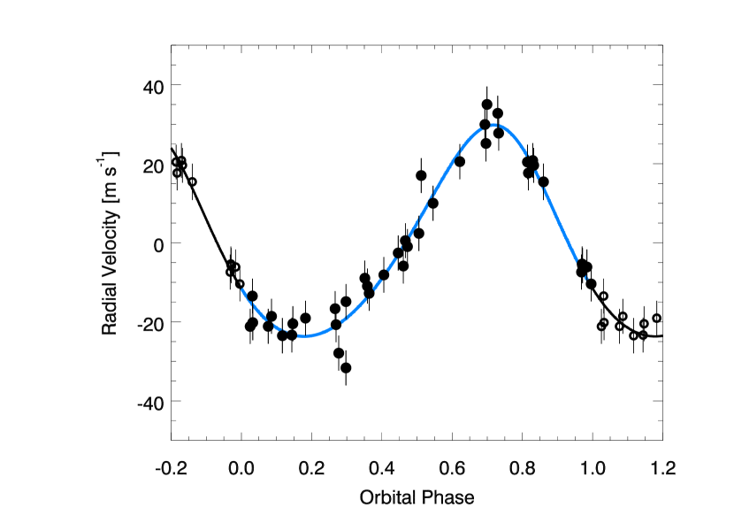
Figure 14.— Phased residual RV measurements for HD 75784 using the $341.7$ orbital period for the inner planet (black) after removing the theoretical model for the outer planet. The blue line shows the best fit Keplerian model for the innner planet. This shows excellent phase coverage for this solution.

Fitting the RV measurements with KFME resulted in an orbital period of $341.7$ $\pm$ $6.1$ days and velocity semi-amplitude of $26.7$ $\pm$ $6.6$ m s^-1 for the well-constrained inner planet. Adding the Isaacson & Fischer (2010) estimated jitter of 4.3 m s^-1 in quadrature to the internal measurement uncertainty resulted in a goodness of fit measurement of 1.25, indicating appropriate estimates for both the jitter and the internal uncertainty. Adopting a stellar mass of $1.41$ $M_{\odot}$, we derive a semi-major axis of $1.073$ $\pm$ $0.013$ AU and a minimum mass of $1.15$ $\pm$ $0.30$ $M_{\rm Jup}$ for the inner planet. Figure 13 shows the radial velocity measurements of HD 75784 with the double planet model superimposed in blue. Figure 14 shows the phased model for the inner planet after subtracting the Keplerian model for the outer planet. The Keplerian model for the inner planet was then superimposed in blue, and it can be seen that there is excellent phase coverage. After fitting for both the inner planet and poorly-constrained outer planet, there were no significant signals in the residuals, which can be seen in Figure 15. The full orbital solution is summarized in Table 7.

Table 7Orbital Parameters for the HD 75784 System

Parameter	HD 75784 b	Outer Companion
P(d)	$341.7$ $\pm$ $6.1$	$5040$ $\pm$ $3414$
TP(JD)	$14411$ $\pm$ $172$	$19655$ $\pm$ $2297$
e	$0.13$ $\pm$ $0.10$	$0.36$ $\pm$ $0.16$
$\omega$	$29$ $\pm$ $136$	$301$ $\pm$ $75$
K (m s-1)	$26.7$ $\pm$ $6.6$	$57$ $\pm$ $11$
a (au)	$1.073$ $\pm$ $0.013$	$6.5$ $\pm$ $2.0$
M $\sin{i}$ ($M_{\rm Jup}$)	$1.15$ $\pm$ $0.30$	$5.6$ $\pm$ $1.2$
N${}_{\textrm{obs}}$	$41$
Jitter (m s-1)	$4.3$
rms (m s-1)	$4.63$
$\chi_{\nu}^{2}$	$1.09$

Figure 15.— Periodogram of the residuals for HD 75784 after removing the 2 planet Keplerian model. The false alarm probability levels of 10 % (solid) and 1% (dotted) are superimposed showing there is no strong periodic signal remaining. This agrees well with our final goodness of fit, showing we did not over-estimate our uncertainty.

Similar to the HD 5319 and HD 11506 S-value analysis, we carried out a GLS periodogram analysis of the S-values for the HD 75784 observations. The S-value time series and periodogram are shown in Figure 16, where it can be seen that there is power at neither the 342-day nor the 5040-day signals. We also searched for a correlation between the RV measurements and the S-values, resulting in a Pearson correlation coefficient of -0.06 with a p-value of 0.73, indicating there is no correlation between the two parameters.

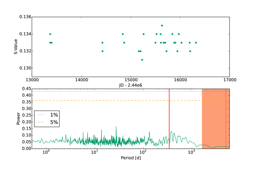
Figure 16.— Same as Figure 2, but for HD 75784 observations. This shows that there is no indication that the observed signals are related to magnetic activity.

Table 8RV Measurements of HD 75784

JD	RV	$\sigma_{RV}$	$S_{HK}$
-2440000	(m s-1)	(m s-1)
13014.9237	-34.09	1.44
13015.9202	-38.90	1.41
13016.9263	-29.04	1.44
13071.8866	-49.56	1.59
13369.0450	-35.73	1.01	0.133
13369.9123	-40.75	1.06	0.134
13397.9009	-48.22	0.82	0.133
13398.8612	-51.00	0.92	0.133
14428.0495	9.88	0.90	0.133
14429.0012	8.81	0.91	0.132
14839.0403	20.02	1.11	0.134
14867.8771	18.26	1.16	0.133
15164.0797	36.49	1.04	0.132
15198.9817	22.88	0.98	0.132
15231.9936	21.20	1.00	0.131
15260.7745	22.45	0.99	0.134
15501.0661	22.23	1.05	0.133
15522.0041	13.04	1.01	0.134
15606.0111	-5.78	1.02	0.134
15613.0127	-9.88	1.01	0.133
15633.8478	9.72	0.98	0.135
15663.8356	16.54	0.93	0.133
15668.8324	12.99	1.03	0.133
15670.7782	19.29	0.91	0.133
15672.8363	17.69	0.95	0.133
15697.7436	27.37	0.99	0.133
15723.7403	36.56	1.07	0.132
15842.1218	2.62	1.06	0.134
15843.0915	4.20	1.13	0.100
15879.0679	-12.94	0.95	0.133
15902.0401	-16.28	0.90	0.133
15902.9937	-13.46	1.03	0.133
15945.0258	-15.73	1.08	0.132
15973.0361	-5.31	1.08	0.134
16027.8576	18.07	0.98	0.133
16193.1420	-16.85	0.94	0.133
16203.1417	-28.03	0.99	0.132
16318.8825	-24.60	0.88	0.133
16638.0095	-39.22	1.04
16674.8593	-33.82	1.33
16708.9338	-24.55	1.10

7. HD 10442

7.1. Stellar Characteristics

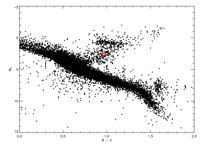
Figure 17.— HR diagram of the stars within 50 pc from the $Hipparcos$ Catalog. Superimposed in red are the stars used to estimate the mass of HD 10442.

As stated in §2, the N2K sample was selected from the $Hipparcos$ Catalog. Since HD 10442 (TYC 32-383-1) is not a member of the $Hipparcos$ catalog, this star is likely one of a few metal-rich stars that were added to the target list as part of an undergraduate research project. Without knowing the distance to HD 10442, we could not iterate between the $Y^{2}$ isochrones and SME as described in §3, and therefore do not have values for the stellar mass, luminosity, age, or stellar radius as we do for the other 3 stars presented in this work. The stellar characteristics calculated using the non-iterative form of SME for HD 10442 are $\log g$ = $3.50$ $\pm$ $0.06$, $T_{\rm eff}$ = $5034$ $\pm$ $44$ K, and [Fe/H] = $0.11$ $\pm$ $0.03$.

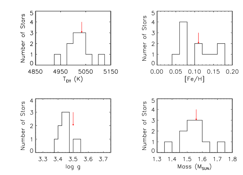
Figure 18.— $T_{\rm eff}$, [Fe/H], $\log g$, and mass distributions for the 11 stars within 2-$\sigma$ of the $T_{\rm eff}$, , [Fe/H], and $\log g$ of HD 10442. The red arrows show the values for HD 10442.

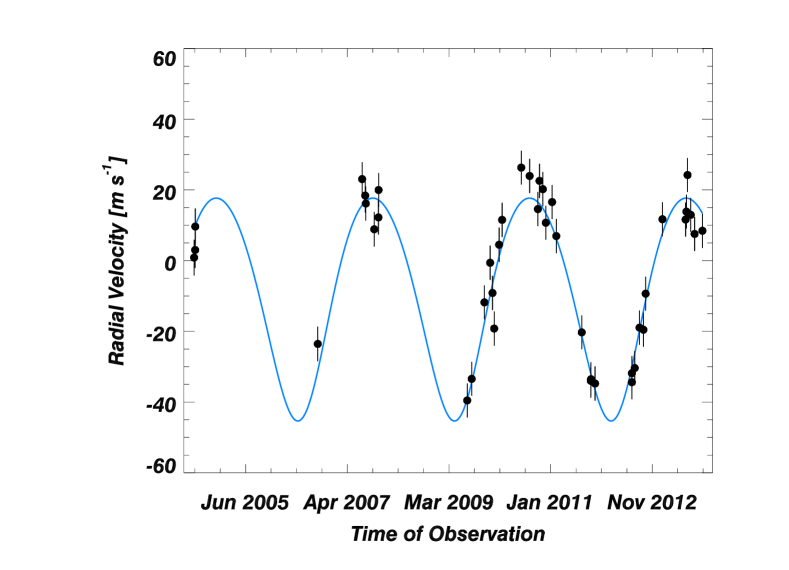
Figure 19.— Radial velocity measurements for HD 10442 with associated errors (black) and the best-fit Keplerian model superimposed in blue.

To estimate the stellar mass of HD 10442, we searched our SME analysis of stars that were within 2-$\sigma$ of the SME derived $\log g$, [Fe/H], and $T_{\rm eff}$ of HD 10442. The resulting 11 stars satisfying the 2-$\sigma$ criteria are shown in red in Figure 17 amongst all stars in the $Hipparcos$ Catalog that are within 50 pc of the Sun. The median stellar mass of the 11 star sample ($1.56$ $M_{\odot}$) and standard deviation ($0.09$) were adopted for the mass and associated uncertainty of HD 10442 when calculating the orbital parameters of HD 10442 b. Figure 18 shows the $T_{\rm eff}$, [Fe/H], $\log g$, and stellar masses of these 11 stars, and the red arrows show the values for HD 10442.

The Tycho B_T and V_T magnitudes for HD 10442 are 9.06 and 7.94, respectively. Converting to Johnson magnitudes gives V = 7.84 and B - V = 0.93. SIMBAD lists HD 10442 as a G5 star of unknown luminosity class. Based on the stellar parameters derived using SME, the B and V values from Tycho, and the position on the HR diagram, this star most closely resembles a K2 subgiant. We therefore adopt a jitter value of 4.7 m s^-1 from Isaacson & Fischer (2010). The stellar parameters for HD 10442 are summarized in Table 2.

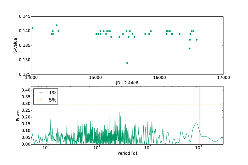
Figure 20.— Same as Figure 2, but for S-values of HD 10442 observations. This shows that there is no significant magnetic activity signal.

7.2. Doppler Observations & Orbital Solution

HD 10442 was first observed with the HIRES spectrometer at Keck Observatory in July of 2004. Although it was clear after the first few observations that this star did not harbor a hot Jupiter, the velocities showed a significant linear trend. HD 10442 was therefore kept on the active observing program. Now, with a time baseline of Doppler measurements spanning more than 10 years, the planetary nature of this signal has been confirmed.

The orbital solution that best fits the Doppler measurements has an orbital period of $1043$ $\pm$ $9$ days, an eccentricity of $0.11$ $\pm$ $0.06$, and semi-amplitude of $31.5$ $\pm$ $2.2$ m s^-1. Using these parameters and assuming a stellar mass of $1.56$ $M_{\odot}$, we calculate a minimum mass of $2.10$ $\pm$ $0.15$ $M_{\rm Jup}$ and a semi-major axis of $2.335$ $\pm$ $0.014$ AU for the planetary companion. Figure 19 shows the full set of radial velocity measurements and the best-fit single-planet orbital solution is superimposed with a solid blue line. Both the periodogram and Keplerian FAP analyses give an FAP of $<$ 0.1% for HD 10442 b.

As with the other systems, periodogram analysis of the S-values for the HD 10442 observations (shown in Figure 20) reveals no significant power due to magnetic activity. A search for a linear correlation between the RV measurements results in a Pearson correlation coefficient of -0.28 with a corresponding p-value of 0.08 – again showing no significant correlation between the two parameters – supporting the planetary interpretation.

Figure 21.— Periodogram for the residuals of HD 10442 after subtracting the best-fit model, Superimposed are FAP levels of 10 % (solid), 1% (dotted) and 0.1% (dashed). This shows a signal with a period of $\sim$ 2 days, but with a high FAP indicating it is most likely due to a window function in the time series data.

Figure 22.— Best-fit $\chi_{\nu}^{2}$ distribution after performing a bootstrap Monte Carlo scrambling of the residual velocities to the 2 planet fit for HD 10442, then refitting with a Keplerian model. $>$80% of the 10,000 realizations resulted in a lower $\chi_{\nu}^{2}$ than the unscrambled velocities, reiterating the periodogram FAP analysis result that the 2-day signal is a window function in the data.

Analysis of the residuals to this single-planet solution shows a spike of power in the residuals corresponding to a period of $\sim$ 2 days. However, Figures 21 and 22 show that the periodogram and Keplerian FAP tests both give a high FAP for this period. Furthermore, the $\chi_{\nu}^{2}$ did not improve when including the 2 day signal in the orbital solution. This leads us to conclude that this 2 day signal is not due to the presence of an additional companion, but rather a window function in our radial velocity set. The full orbital solution for HD 10442 b is summarized in Table 9.

Table 9Orbital Parameters for the HD 10442 System

Parameter	HD 10442 b
P(d)	$1043$ $\pm$ $9$
TP(JD)	$17062$ $\pm$ $770$
e	$0.11$ $\pm$ $0.06$
$\omega$	$198$ $\pm$ $60$
K (m s-1)	$31.5$ $\pm$ $2.2$
a (au)	$2.335$ $\pm$ $0.014$
M$\sin{i}$ ($M_{\rm Jup}$)	$2.10$ $\pm$ $0.15$
N${}_{\textrm{obs}}$	$43$
Jitter (m s-1)	$4.7$
rms (m s-1)	$5.98$
$\chi_{\nu}^{2}$	$1.53$

8. Summary & Discussion

Here we have presented 4 newly-discovered exoplanets (HD 5319 c, HD 11506 c, HD 75784 b and HD 10442 b), refined orbital parameters for 2 previously published planets (HD 5319 b and HD 11506 b), and have shown indications that two more companions may exist (orbiting HD 11506, HD 75784) but need additional observations to constrain their orbital parameters. Two of these stars (HD 5319 and HD 11506) were already known to harbor single gas giant planets. These two systems have therefore transitioned from the ensemble of known single-planet systems to multi-planet systems. The detection of additional planets orbiting these stars supports the result of Wright et al. (2009a), where they found that the most probable multi-planet systems are systems where single planets have already been detected.

HD 5319 is a remarkable system due to its unknown formation mechanism. Through hydrodynamical simulations Rein et al. (2012) have shown that massive planets cannot form in situ in the 4:3 resonance. Instead, these planets must have undergone migration to get to their current positions. However, Rein et al. (2012) went on to show that convergent migration also fails to create high mass planetary systems in 4:3 resonances because unphysical migration rates are needed to overcome the more widely separated first order resonances. In the same work Rein et al. (2012) also showed that it is unlikely that the number of observed gas giant systems in the 4:3 resonance could have been created through planet-planet scattering. While they suggest two unexplored possibilities for the formation of high mass planets in 4:3 MMRs, the formation mechanism of the HD 5319 system is currently an open problem.

HD 11506 has also been promoted to multi-planet status. The outer planet orbiting HD 11506 was first announced by Fischer et al. (2007). Fischer et al. (2007) also commented that several peaks existed in the periodogram of the residuals, including a peak in the power at 170 days; however, they stated more data were needed to evaluate the second-signal. Reanalyzing the RV measurements from that work, Tuomi & Kotiranta (2009) claimed the period of the second planet was 170.5${}^{+3.3}_{-6.2}$ with 99% confidence. With the additional 87 observations presented in this work, we find an orbital period for the second planet of $223.6$ $\pm$ $0.6$ days, which is significantly different than 170-day signal that was starting to become apparent in the previously-published data set by Fischer et al. (2007). The best-fit solution now has two planets with well-constrained orbital parameters and a distant third companion approximated as a linear contribution to the radial velocity measurements.

Table 10RV Measurements of HD 10442

JD	RV	$\sigma_{RV}$	$S_{HK}$
-2440000	(m s-1)	(m s-1)
13200.0655	0.86	1.83
13207.0955	3.01	1.75
13208.0761	9.64	2.02
14024.0035	-23.56	1.24	0.141
14319.0890	23.06	0.78	0.139
14339.9948	18.39	0.99	0.140
14343.9694	16.15	0.98	0.139
14399.9071	8.86	1.29	0.142
14427.9188	12.22	0.99	0.140
14428.8102	19.97	0.94	0.140
15019.1203	-39.55	0.99	0.139
15049.1033	-33.44	0.94	0.139
15133.9656	-11.80	0.99	0.140
15171.8824	-0.61	1.12	0.139
15187.8836	-9.16	1.04	0.140
15198.8405	-19.21	1.04	0.140
15231.7423	4.49	1.07	0.140
15251.7110	11.53	1.05	0.138
15379.1166	26.31	0.89	0.138
15435.1172	23.94	0.99	0.139
15489.9581	14.58	1.08	0.140
15500.8787	22.56	1.01	0.129
15522.9023	20.21	1.09	0.138
15542.9554	10.71	0.96	0.140
15584.7897	16.57	1.01	0.139
15612.7098	6.95	1.08	0.138
15782.1119	-20.30	0.92	0.139
15841.9779	-33.99	0.95	0.139
15843.9846	-33.55	0.94	0.139
15870.9958	-34.75	1.13	0.140
16116.1286	-34.38	1.20	0.140
16116.1295	-31.85	1.16	0.139
16135.1267	-30.37	0.98	0.140
16167.1030	-18.96	1.12	0.140
16193.1258	-19.54	1.00	0.139
16207.9660	-9.35	0.95	0.139
16319.7270	11.70	0.96	0.139
16474.1247	11.62	1.00	0.134
16479.1294	13.86	0.89	0.137
16487.1288	24.21	0.95	0.139
16508.1309	12.95	0.91	0.140
16534.0526	7.54	0.97	0.140
16585.9211	8.44	1.13	0.137

An interesting characteristic of the HD 11506 system is the linear correlation between the residual velocities after subtracting the 2-planet + linear trend model and the S-values. Subtracting this magnetic signal from the velocities and refitting the system had no significant effect on the best-fit orbital parameters, but it did lower the rms by 1.0 m s^-1. This emphasizes the need for sophisticated methods to handle stellar activity when searching for low mass planets.

A planet has also been discovered orbiting HD 75784, which was not known to host any planets prior to this work. To properly model the radial velocity measurements of HD 75784, a second (longer period) Keplerian signal needed to be included. However, the time baseline of our radial velocity measurements is shorter than the orbital period for the outer planet leading to a poorly-constrained orbital solution using both frequentist and Bayesian approaches. Although the orbital solution for the outer planet is poorly constrained, the solution for the inner planet is well-known and warrants publication at this time. HD 75784 will remain an active target to constrain the orbital parameters for the outer planet. The current best-fit solution for the outer planet has a semi-major axis of $\sim$6.5 AU, making it one of the most widely-separated planets discovered with the radial velocity technique. An interesting characteristic of HD 75784 is that it has an abnormally low [Si/Fe] of -0.16 $\pm$ 0.05. Brugamyer et al. (2011) found that gas giants are preferentially detected orbiting stars that are enhanced in silicon relative to iron, making the HD 75784 system a curious outlier to their observations.

Lastly, the we announced a single gas giant orbiting HD 10442. Unlike the rest of the stars discussed in this work, HD 10442 does not have a $Hipparcos$ parallax measurement and we could therefore not use the $Y^{2}$ isochrones to determine its mass. To calculate the mass of HD 10442 b, we instead used the median mass of stars from a modified SPOCS catalog that are similar to HD 10442 in [Fe/H], $T_{\rm eff}$ and $\log g$.

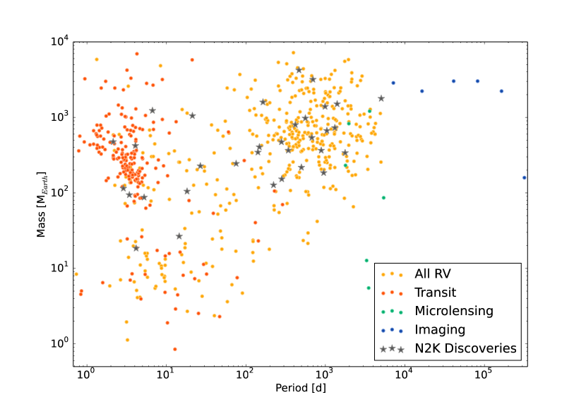
Figure 23.— All confirmed planets listed on exoplanets.org. Planets discovered using the transit, RV, microlensing, and direct imaging techniques are shown in red, orange, green, and blue circles, respectively. Superimposed in gray stars are the planets discovered through the N2K Consortium.

These discoveries bring the total number of planets detected through the N2K Consortium to 32. The original goal of the N2K was to detect short-period gas giants, which have high transit probabilities. It has since evolved into a campaign to detect long-period planets. The full ensemble of planets discovered through the N2K Program is shown in Figure 23 (gray star symbols) amidst all known exoplanets listed on exoplanets.org. This shows the wide-range of mass-period parameter space covered by planets discovered through this program. Included as a member of the N2K detections in Figure 23 is the candidate HD 75784 c. While this outer companion orbiting HD 75784 is still poorly-constrained, additional observations of this target, and many others that are from the original pool of stars observed as part of N2K, will help build a large population of widely separated planets discovered with the radial velocity method. Building a large population of such widely separated systems will be useful for the future comparison of the occurrence rate of planets discovered using the direct imaging method and radial velocity method, and to refine population synthesis models to improve our understanding of planet migration.

References

- Albrecht et al. (2013) Albrecht, S., Setiawan, J., Torres, G., Fabrycky, D. C., & Winn, J. N. 2013, ApJ, 767, 32
- Alibert et al. (2013) Alibert, Y., Carron, F., Fortier, A., et al. 2013, A&A, 558, 109
- Ammons et al. (2006) Ammons, S. M., Robinson, S. E., Strader, J., et al. 2006, ApJ, 638, 1004
- Anderson & Adams (2012) Anderson, K. R., & Adams, F. C. 2012, PASP, 124, 809
- Barbieri et al. (2007) Barbieri, M., Alonso, R., Laughlin, G., et al. 2007, A&A, 476, L13
- Batalha et al. (2013) Batalha, N. M., Rowe, J. F., Bryson, S. T., et al. 2013, ApJS, 204, 24
- Bate et al. (2010) Bate, M. R., Lodato, G., & Pringle, J. E. 2010, MNRAS, 401, 1505
- Batygin (2012) Batygin, K. 2012, Nature, 491, 418
- Beuzit et al. (2008) Beuzit, J.-L., Feldt, M., Dohlen, K., et al. 2008, Proc. SPIE, 7014, 41
- Borucki et al. (2011) Borucki, W. J., Koch, D. G., Basri, G., et al. 2011, ApJ, 728, 117
- Brugamyer et al. (2011) Brugamyer, E., Dodson-Robinson, S. E., Cochran, W. D., & Sneden, C. 2011, ApJ, 738, 97
- Butler et al. (1996) Butler, R. P., Marcy, G. W., Williams, E., et al. 1996, PASP, 108, 500
- Cassan et al. (2012) Cassan, A., Kubas, D., Beaulieu, J. P., et al. 2012, Nature, 481, 167
- Chambers (1999) Chambers, J. E. 1999, MNRAS, 304, 793
- Chatterjee et al. (2008) Chatterjee, S., Ford, E. B., Matsumura, S., & Rasio, F. A. 2008, ApJ, 686, 580
- Demarque et al. (2004) Demarque, P., Woo, J.-H., Kim, Y.-C., & Yi, S. K. 2004, ApJS, 155, 667
- Dodson-Robinson & Bodenheimer (2009) Dodson-Robinson, S. E., & Bodenheimer, P. 2009, ApJL, 695, L159
- Dumusque et al. (2011) Dumusque, X., Santos, N. C., Udry, S., Lovis, C., & Bonfils, X. 2011, A&A, 527, 82
- ESA (1997) ESA. 1997, VizieR Online Data Catalog, 1239, 0
- Fabrycky & Tremaine (2007) Fabrycky, D., & Tremaine, S. 2007, ApJ, 669, 1298
- Fischer & Valenti (2005) Fischer, D. A., & Valenti, J. 2005, ApJ, 622, 1102
- Fischer et al. (2005) Fischer, D. A., Laughlin, G., Butler, P., et al. 2005, ApJ, 620, 481
- Fischer et al. (2006) Fischer, D. A., Laughlin, G., Marcy, G. W., et al. 2006, ApJ, 637, 1094
- Fischer et al. (2007) Fischer, D. A., Vogt, S. S., Marcy, G. W., et al. 2007, ApJ, 669, 1336
- Ford & Rasio (2008) Ford, E. B., & Rasio, F. A. 2008, ApJ, 686, 621
- Fortney et al. (2005) Fortney, J. J., Saumon, D., Marley, M. S., Lodders, K., & Freedman, R. S. 2005, arXiv, 495
- Giguere et al. (2012) Giguere, M. J., Fischer, D. A., Howard, A. W., et al. 2012, ApJ, 744, 4
- Goldreich & Tremaine (1980) Goldreich, P., & Tremaine, S. 1980, ApJ, 241, 425
- Gonzalez (1997) Gonzalez, G. 1997, MNRAS, 285, 403
- Gray (2008) Gray, D. F. 2008, The Observation and Analysis of Stellar Photospheres, 3rd edn., Vol. -1 (Cambridge, UK: The Observation and Analysis of Stellar Photospheres, by David F. Gray, Cambridge, UK: Cambridge University Press, 2008)
- Greaves et al. (2014) Greaves, J. S., Kennedy, G. M., Thureau, N., et al. 2014, Monthly Notices of the Royal Astronomical Society: Letters, 438, L31
- Harakawa et al. (2010) Harakawa, H., Sato, B., Fischer, D. A., et al. 2010, ApJ, 715, 550
- Hartung et al. (2013) Hartung, M., Macintosh, B., Poyneer, L., et al. 2013, arXiv, 1311.4423v1
- Howard et al. (2009) Howard, A. W., Johnson, J. A., Marcy, G. W., et al. 2009, ApJ, 696, 75
- Ida & Lin (2004) Ida, S., & Lin, D. N. C. 2004, ApJ, 604, 388
- Ida et al. (2013) Ida, S., Lin, D. N. C., & Nagasawa, M. 2013, ApJ, 775, 42
- Isaacson & Fischer (2010) Isaacson, H., & Fischer, D. 2010, ApJ, 725, 875
- Ivezić et al. (2013) Ivezić, Z., Connolly, A., VanderPlas, J., & Gray, A. 2013, Princeton Series in Modern Observational Astronomy, Vol. -1, Statistics, Data Mining, and Machine Learning in Astronomy (Statistics, Data Mining, and Machine Learning in Astronomy, by Ż. Ivezić et al. Princeton University Press, 2013)
- Johnson (1966) Johnson, H. L. 1966, ARA&A, 4, 193
- Johnson et al. (2007) Johnson, J. A., Butler, R. P., Marcy, G. W., et al. 2007, ApJ, 670, 833
- Johnson et al. (2006) Johnson, J. A., Marcy, G. W., Fischer, D. A., et al. 2006, ApJ, 647, 600
- Johnson et al. (2011) Johnson, J. A., Payne, M., Howard, A. W., et al. 2011, AJ, 141, 16
- Knutson et al. (2013) Knutson, H. A., Fulton, B. J., Montet, B. T., et al. 2013, arXiv, 1312.2954v1
- Lai et al. (2011) Lai, D., Foucart, F., & Lin, D. N. C. 2011, MNRAS, 412, 2790
- Lewis et al. (2011) Lewis, N. K., Showman, A. P., Fortney, J. J., Marley, M. S., & Freedman, R. S. 2011, Molecules in the Atmospheres of Extrasolar Planets, 450, 71
- Lin et al. (1996) Lin, D. N. C., Bodenheimer, P., & Richardson, D. C. 1996, Nature, 380, 606
- Lissauer (1993) Lissauer, J. J. 1993, ARA&A, 31, 129
- Lissauer et al. (2011) Lissauer, J. J., Ragozzine, D., Fabrycky, D. C., et al. 2011, ApJS, 197, 8
- López-Morales et al. (2008) López-Morales, M., Butler, R. P., Fischer, D. A., et al. 2008, AJ, 136, 1901
- Lovis et al. (2011) Lovis, C., Dumusque, X., Santos, N. C., et al. 2011, arXiv, 5325
- Marcy & Butler (1996) Marcy, G. W., & Butler, R. P. 1996, ApJL, 464, L147
- Marcy et al. (2005) Marcy, G. W., Butler, R. P., Vogt, S. S., et al. 2005, ApJ, 619, 570
- Mayor & Queloz (1995) Mayor, M., & Queloz, D. 1995, Nature, 378, 355
- Nelson et al. (2013) Nelson, B. E., Ford, E. B., & Payne, M. J. 2013, arXiv, 1311.5229v1
- Noyes et al. (1984) Noyes, R. W., Hartmann, L. W., Baliunas, S. L., Duncan, D. K., & Vaughan, A. H. 1984, ApJ, 279, 763
- Peek et al. (2009) Peek, K. M. G., Johnson, J. A., Fischer, D. A., et al. 2009, PASP, 121, 613
- Pollack et al. (1996) Pollack, J. B., Hubickyj, O., Bodenheimer, P., et al. 1996, Icarus, 124, 62
- Press et al. (1992) Press, W. H., Teukolsky, S. A., Vetterling, W. T., & Flannery, B. P. 1992, Numerical Recipes in C: The Art of Scientific Computer, 2nd edn. (Cambridge University Press)
- Rein et al. (2012) Rein, H., Payne, M. J., Veras, D., & Ford, E. B. 2012, MNRAS, 426, 187
- Robinson et al. (2007) Robinson, S. E., Laughlin, G., Vogt, S. S., et al. 2007, ApJ, 670, 1391
- Saar & Donahue (1997) Saar, S. H., & Donahue, R. A. 1997, Astrophysical Journal v.485, 485, 319
- Saar & Fischer (2000) Saar, S. H., & Fischer, D. 2000, ApJ, 534, L105
- Santos et al. (2010) Santos, N. C., Gomes da Silva, J., Lovis, C., & Melo, C. 2010, A&A, 511, 54
- Santos et al. (2004) Santos, N. C., Israelian, G., & Mayor, M. 2004, A&A, 415, 1153
- Sato et al. (2005) Sato, B., Fischer, D. A., Henry, G. W., et al. 2005, ApJ, 633, 465
- Sato et al. (2009) Sato, B., Fischer, D. A., Ida, S., et al. 2009, ApJ, 703, 671
- Schlaufman (2010) Schlaufman, K. C. 2010, ApJ, 719, 602
- Tuomi & Kotiranta (2009) Tuomi, M., & Kotiranta, S. 2009, A&A, 496, L13
- Valenti et al. (1995) Valenti, J. A., Butler, R. P., & Marcy, G. W. 1995, PASP, 107, 966
- Valenti & Fischer (2005) Valenti, J. A., & Fischer, D. A. 2005, ApJS, 159, 141
- Valenti & Piskunov (1996) Valenti, J. A., & Piskunov, N. 1996, A&AS, 118, 595
- Valenti et al. (2009) Valenti, J. A., Fischer, D., Marcy, G. W., et al. 2009, ApJ, 702, 989
- van Leeuwen (2007) van Leeuwen, F. 2007, A&A, 474, 653
- VandenBerg & Clem (2003) VandenBerg, D. A., & Clem, J. L. 2003, AJ, 126, 778
- Vogt et al. (1994) Vogt, S. S., Allen, S. L., Bigelow, B. C., et al. 1994, in Proc. SPIE, ed. D. L. Crawford & E. R. Craine (SPIE), 362–375
- Winn et al. (2010) Winn, J. N., Fabrycky, D., Albrecht, S., & Johnson, J. A. 2010, ApJL, 718, L145
- Winn et al. (2005) Winn, J. N., Noyes, R. W., Holman, M. J., et al. 2005, ApJ, 631, 1215
- Wright et al. (2009a) Wright, J. T., Upadhyay, S., Marcy, G. W., et al. 2009a, ApJ, 693, 1084
- Wright et al. (2007) Wright, J. T., Marcy, G. W., Fischer, D. A., et al. 2007, ApJ, 657, 533
- Wright et al. (2009b) Wright, J. T., Fischer, D. A., Ford, E. B., et al. 2009b, ApJL, 699, L97
- Wu & Lithwick (2011) Wu, Y., & Lithwick, Y. 2011, ApJ, 735, 109
- Wu & Murray (2003) Wu, Y., & Murray, N. 2003, ApJ, 589, 605