The Relation between Dynamical Mass-to-Light Ratio and Color for Massive Quiescent Galaxies out to $z\sim 2$ and Comparison with Stellar Population Synthesis Models

Abstract

We explore the relation between the dynamical mass-to-light ratio ($M/L$) and rest-frame color of massive quiescent galaxies out to $z\sim 2$. We use a galaxy sample with measured stellar velocity dispersions in combination with Hubble Space Telescope and ground-based multi-band photometry. Our sample spans a large range in $\log M_{\rm{dyn}}/L_{\rm{g}}$ (of 1.6 dex) and $\log~{}M_{\rm{dyn}}/L_{\rm{K}}$ (of 1.3 dex). There is a strong, approximately linear correlation between the $M/L$ for different wavebands and rest-frame color. The root-mean-scatter scatter in $\log~{}M_{\rm{dyn}}/L$ residuals implies that it is possible to estimate the $M/L$ with an accuracy of $\sim 0.25$ dex from a single rest-frame optical color. Stellar population synthesis (SPS) models with a Salpeter stellar initial mass function (IMF) can not simultaneously match $M_{\rm{dyn}}/L_{\rm{g}}$ vs. $(g-z)_{\rm{rest-frame}}$ and $M_{\rm{dyn}}/L_{\rm{K}}$ vs. $(g-K)_{\rm{rest-frame}}$. By changing the slope of the IMF we are still unable to explain the M/L of the bluest and reddest galaxies. We find that an IMF with a slope between $\alpha=2.35$ and $\alpha=1.35$ provides the best match. We also explore a broken IMF with a Salpeter slope at $M<1M_{\odot}$ and $M>4M_{\odot}$ and a slope $\alpha$ in the intermediate region. The data favor a slope of $\alpha=1.35$ over $\alpha=2.35$. Nonetheless, our results show that variations between different SPS models are comparable to the IMF variations. In our analysis we assume that the variation in $M/L$ and color is driven by differences in age, and that other contributions (e.g., metallicity evolution, dark matter) are small. These assumptions may be an important source of uncertainty as galaxies evolve in more complex ways.

1. Introduction

For a good understanding of galaxy evolution, accurate stellar mass estimates are crucial (for a recent review see Courteau et al. 2014). Nearly all galaxy properties, among which structure, star formation activity, and the chemical enrichment history are strongly correlated with the stellar mass (e.g., Kauffmann et al. 2003; Tremonti et al. 2004; Gallazzi et al. 2005). Furthermore, the evolution of the stellar mass function (e.g., Bundy et al. 2006; Marchesini et al. 2009; Muzzin et al. 2013b; Ilbert et al. 2013) provides strong constraints on galaxy formation models (see e.g., De Lucia & Blaizot 2007).

In contrast to the luminosity, the stellar mass of a galaxy is not a direct observable quantity. Most techniques for estimating the stellar mass rely on a determination of a mass-to-light ratio. The $M/L$ of a galaxy strongly depends on the age, metallicity, and the stellar initial mass function (IMF) of its stellar population. $M/L$ are typically estimated by comparing the observed colors, multi-wavelength broadband photometry or spectra to stellar population synthesis (SPS) models (for a review see Conroy 2013).

In this Paper, we focus on the relation between the $M/L$ and color, as was first explored by Bell & de Jong (2001). They used SPS models and derived a tight relation between rest-frame $B-R$ color and $M/L_{\rm B}$, from which it is possible to estimate the $M/L$ of a galaxy to an accuracy of $\sim 0.2$ dex. Because their results were based on SPS models, they suffer from uncertainties due to assumptions regarding the star formation history (SFH), metallicity, IMF, and SPS code. More recent work indeed suggests that the uncertainties are larger (0.2-0.4 dex; Bell et al. 2003; Zibetti et al. 2009; Taylor et al. 2011), in particular when using rest-frame NIR colors.

Table 1Data References Sample

SDSS DR7 & 4621 $0.05<z<0.07$ Abazajian et al. (2009) SDSS Blanton et al. (2005) Simard et al. (2011)

NMBS-COSMOS 3 $0.7<z<0.9$ Bezanson et al. (2013) Keck-DEIMOS Skelton et al. (2014) Bezanson et al. (2011)
10 Whitaker et al. (2011)

UKIDSS-UDS 3 $0.6<z<0.7$ Bezanson et al. (2013) Keck-DEIMOS Skelton et al. (2014) van der Wel et al. (2012)
1 Williams et al. (2009)

MS 1054-0321 8 $z=0.83$ Wuyts et al. (2004) Keck-LRIS Förster Schreiber et al. Blakeslee et al. (2006)
2006
GOODS-S 7 $0.9<z<1.2$ van der Wel et al. (2005) VLT-FORS2 Skelton et al. (2014) van der Wel et al. (2012)

GOODS-N 1 $z=1.315$ Newman et al. (2010) Keck-LRIS Skelton et al. (2014) van der Wel et al. (2012)

EGS 8 $1.0<z<1.3$ Belli et al. (2014a) Keck-LRIS Skelton et al. (2014) van der Wel et al. (2012)
COSMOS 6 $1.1<z<1.3$ Belli et al. (2014a) Keck-LRIS Skelton et al. (2014) van der Wel et al. (2012)
GOODS-S 1 $z=1.419$ Belli et al. (2014a) Keck-LRIS Skelton et al. (2014) van der Wel et al. (2012)

NMBS-COSMOS 4 $1.2<z<1.5$ Bezanson et al. (2013a) Keck-LRIS Whitaker et al. (2011) Bezanson et al. (2013a)
NMBS-AEGIS 2 $1.4<z<1.6$ Bezanson et al. (2013a) Keck-LRIS Whitaker et al. (2011) Bezanson et al. (2013a)

NMBS–COSMOS 2 $1.6<z<2.1$ van de Sande et al. (2013) VLT-XShooter Skelton et al. (2014) van de Sande et al. (2013)
1 Whitaker et al. (2011)
UKIDSS-UDS 1 $1.4<z<2.1$ van de Sande et al. (2013) VLT-XShooter Skelton et al. (2014) van de Sande et al. (2013)
1 Williams et al. (2009)

COSMOS 1 $z=1.823$ Onodera et al. (2012) Subaru-MOIRCS Muzzin et al. (2013a) Onodera et al. (2012)
MUSYC 1255 1 $z=2.286$ van Dokkum et al. (2009)Gemini-GNIRS Blanc et al. (2008) van Dokkum et al. (2009)

COSMOS 2 $2.1<z<2.3$ Belli et al. (2014b) Keck-MOSFIRE Skelton et al. (2014) Belli et al. (2014b)

Table 2Absolute Magnitudes of the Sun in different Filters

6.34 & 5.33 4.81 4.65 4.55 6.45 5.14 4.65 4.54 4.52 4.57 4.71 5.19

Direct stellar kinematic mass measurements yield dynamical $M/L$, which do not rely on any assumptions regarding the SPS models, metallicity, and IMF. At low-redshift, dynamical mass measurements of galaxies have proven to be extremely useful for studying the $M/L$ (e.g, Cappellari et al. 2006; de Jong & Bell 2007; Taylor et al. 2010). For example, Cappellari et al. (2006) find that the stellar $M/L$ is tightly correlated with $\sigma_{e}$, and Taylor et al. (2010) find that the stellar $M/L$ is a good predictor of the dynamical $M/L$ if the the Sérsic index is taken into account when calculating dynamical masses (i.e., $M_{\rm dyn}\propto K(n)r_{\rm e}\sigma_{\rm e}^{2}$). van der Wel et al. (2006) studied the relation between the dynamical $M/L_{\rm K}$ and rest-frame $B-K$ color of early-type galaxies out to $z\sim 1$, and found that there are large discrepancies between different SPS models in the NIR. However, one of the major limitations in this measurement was the low number of galaxies, and the small dynamic range in $M/L_{\rm K}$ ($\sim$0.4 dex).

In order to accurately constrain the relation between the dynamical $M/L$ and color, we need a sample of early-type galaxies with a large range in age. This study requires kinematic measurements from $z\sim 0$ to $z\sim 2$, such that we measure the $M/L$ and color in early-type galaxies with both the oldest ($z\sim 0$) and youngest ($z\sim 2$) stellar populations.

However, due to observational challenges very few such measurements exist. At high-redshift, kinematic studies of quiescent galaxies become much more difficult as the bulk of the stellar light, and stellar absorption features used to measure velocity dispersions, shift into the near-infrared (NIR) (e.g., Kriek et al. 2009). With the advent of fully depleted, high-resistivity CCDs (e.g., Keck-LRIS), and new NIR spectrographs, such as VLT-X-SHOOTER (Vernet et al., 2011), and Keck-MOSFIRE (McLean et al., 2012), it is now possible to obtain rest-frame optical spectra of quiescent galaxies out to $z\sim 2$. For example, Bezanson et al. (2013a) measured accurate dynamical masses for 8 galaxies at $1.2<z<1.6$. Furthermore, in van de Sande et al. (2011; 2013) we obtained stellar kinematic measurements for 5 massive quiescent galaxies up to redshift $z=2.1$ (see also Toft et al. 2012; Belli et al. 2014b). Combined with high-resolution imaging and multi-wavelength catalogs, these recently acquired kinematic measurements increase the dynamic range of the $M/L$ and rest-frame color.

In this paper, we use a sample of massive quiescent galaxies from $z\sim 2$ to $z\sim 0$ with kinematic measurements and multi-band photometry with the aim of exploring the relation between the $M/L$ and rest-frame color, assessing SPS models, and constraining the IMF. The paper is organized as follows. In Section 2 we present our sample of $0.05<z<2.1$ galaxies, discuss the photometric and spectroscopic data, and describe the derived galaxy properties such as effective radii, rest-frame fluxes, and stellar population parameters. In Section 3 we explore the relation between the $M/L$ and the rest-frame color over a large dynamic range for several pass-bands. We compare our $M/L$ vs. rest-frame color to predictions from stellar population models in Section 4. In Section 5 we use the $M/L$ vs. color and stellar population models to constrain the IMF in massive galaxies, as first proposed by Tinsley (1972; 1980; see also van Dokkum 2008a who first applied this technique to measure the IMF out to $z\sim 1$). In Section 6 we compare our results with previous measurements and discus several uncertainties. Finally, in Section 7 we summarize our results and conclusions. Throughout the paper we assume a $\Lambda$CDM cosmology with $\Omega_{\mathrm{m}}$=0.3 $\Omega_{\Lambda}=0.7$, and $H_{0}=70$ km s^-1 Mpc^-1. All broadband data are given in the AB-based photometric system.

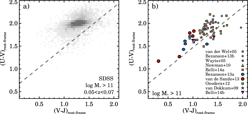
Figure 1.— Rest-frame $U-V$ color vs. $V-J$ color. Panel a) shows massive ($M_{*}>10^{11}$ $M_{\odot}~{}$) galaxies in the SDSS at $z\sim 0.06$, and Panel b) shows massive galaxies at $z>0.5$. Different symbols for the intermediate to high-redshift samples are indicated in the legend and described in Section 2. The dashed lines shows our separation of star-forming and quiescent galaxies, where quiescent galaxies are selected to have $U-V>(V-J)\times 0.88+0.59$. We only use the quiescent galaxies in the remainder of the Paper.

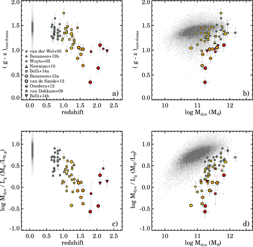
Figure 2.— Panel (a): Rest-frame $g-z$ color vs. redshift. Massive quiescent galaxies in the SDSS at $z\sim 0.06$ are represented by gray squares. Different symbols are the different intermediate to high-redshift samples as indicated in the legend and described in Section 2. Galaxies are color coded by redshift, from low (blue) to high redshift (red). We find that the complete sample has a large range in colors. Panel (b): Rest-frame $g-z$ color versus dynamical mass. Panel (c): $M_{\rm{dyn}}/L_{\rm g}$ in the rest-frame g band vs. redshift. We find that the complete sample has a large dynamic range with a factor of $\sim$25 in $M_{\rm{dyn}}/L_{\rm g}$. Panel (d): $M_{\rm{dyn}}/L_{\rm g}$ versus dynamical mass. Similar to panel b, we color code by redshift. From Panel (a) to (d) we conclude that, within the sample at fixed dynamical mass, the highest-redshift galaxies have the bluest colors with the lowest $M/L$.

2. Data

2.1. Low and High-Redshift Sample

One of the primary goals of this paper is to explore the relation between the $M/L$ and rest-frame color over a large dynamic range. Early-type galaxies are ideal candidates for such a measurement, as they have homogeneous stellar populations. At $z\sim 0$ their spectral energy distributions are dominated by old stellar populations (e.g., Kuntschner et al. 2010), and they have experienced very little to no star formation since $z\sim 2$ (e.g., Kriek et al. 2008).

Here, we use a variety of datasets, which all contain stellar kinematic measurements of individual galaxies and multi-wavelength medium and broad-band photometric catalogs. We adopt a mass limit of $M_{*}>10^{11}$$M_{\odot}~{}$to homogenize the final sample. Our mass-selected sample contains 76 massive galaxies at $0.5<z<2.2$. We note, however, that our sample remains relatively heterogeneous relative to mass-complete photometric samples and in particular the higher redshift samples are biased toward the brightest galaxies.

We use the $U-V$ versus $V-J$ rest-frame color selection to distinguish quiescent galaxies from (dusty) star-forming galaxies. (e.g., Wuyts et al. 2007; Williams et al. 2009). Figure 1 shows the mass selected sample in the UVJ diagram, in which quiescent galaxies have $U-V>(V-J)\times 0.88+0.59$. Out of the 76 galaxies in the mass selected sample, 13 galaxies are not identified as quiescent galaxies and excluded from our sample. This criterion is slightly different from previous work, as we do not require that $U-V>1.3$ or $V-J<1.5$. The latter criteria remove post-starburst galaxies and very old galaxies, respectively. As we benefit from a large range in age in this Paper, we omit the latter criteria and thereby keep the youngest and oldest galaxies in our sample.

Photometry for the high-redshift sample is adopted from the 3D-HST catalogs version 4.1 (Brammer et al. 2012; Skelton et al. 2014) where possible, which cover the following CANDELS fields: AEGIS, COSMOS, GOODS-N, GOODS-S and UKIDSS-UDS. We list the references for all kinematic studies, photometric catalogs, and structural parameters for the final sample in Table 1.

2.2. Derived Galaxy Properties

All velocity dispersions were measured from stellar absorption features in the rest-frame near-UV and/or optical. We apply an aperture correction to the velocity dispersion measurements as if they were observed within a circular aperture radius of one $r_{e}$, following the method as described in van de Sande et al. (2013). This method includes a correction for the radial dependence of the velocity dispersion (e.g., Cappellari et al. 2006), and takes into account the effects of the non-circular aperture, seeing, and optimal extraction of the 1-D spectrum.

For the intermediate to high-redshift sample, effective radii and other structural parameters, such as Sérsic index and axis ratio, are determined using 2D Sérsic fits with GALFIT (Peng et al., 2010). For galaxies in the SDSS, we use the structural parameters from Simard et al. (2011), who determined 2D Sérsic fits with GIMD2D (Simard, 1998) on the SDSS $g$ band imaging data. All effective radii are circularized, i.e., $r_{\rm{e}}=\sqrt{ab}$. All sizes are measured from rest-frame optical data, i.e., redwards of 4000Å, with the exception of COSMOS-13412 ($z=1.24$) from Bezanson et al. (2013a), and COSMOS-254025 ($z=1.82$) from Onodera et al. (2012) for which the HST-F775W band is used. For massive galaxies at $z>1$, the median color gradient is $r_{\rm e,u}/r_{\rm e,g}=1.12$ (Szomoru et al., 2013). Thus the $M/L$ for these two galaxies may be overestimated by $\sim 0.05$ dex.

All rest-frame fluxes, including those for the SDSS sample, are calculated using the photometric redshift code EAZY (v46; Brammer et al. 2008). We use the same set of templates that were used for the ULTRAVISTA catalog by Muzzin et al. (2013a). Stellar masses for the high-redshift sample are derived using the stellar population fitting code FAST (Kriek et al., 2009). We use the Bruzual & Charlot (2003) SPS models and assume an exponentially declining star formation history (SFH), solar metallicity ($Z=0.02$), the Calzetti et al. (2000) dust attenuation law, and the Chabrier (2003) IMF. For galaxies in the SDSS, stellar masses are from the MPA-JHU DR7 release which are based on Brinchmann et al. (2004), assuming a Chabrier (2003) IMF. The photometry and thus also the stellar mass are corrected for missing flux using the best-fit Sérsic luminosity (Taylor et al., 2010).

Dynamical masses are estimated from the size and velocity dispersion measurements using the following expression:

$$M_{\rm dyn}=\frac{\beta(n)~{}\sigma_{\rm e}^{2}~{}r_{\rm e}}{G}.$$ (1)

Here $\beta(n)$ is an analytic expression as a function of the Sérsic index, as described by Cappellari et al. (2006):

$$\beta(n)=8.87-0.831n+0.0241n^{2}.$$ (2)

We note that if we use a fixed virial constant of $\beta=5$ for all galaxies our conclusion would not change.

We derive mass-to-light ratios ($M/L_{\rm{\lambda}}$) using the dynamical mass from Equation 1 divided by the total luminosity, in units of $M_{\odot}L_{\odot,\rm{\lambda}}^{-1}$. The total luminosities for different wave bands ($\lambda$) are calculated from rest-frame fluxes, as derived using EAZY. We normalize the total luminosity using the absolute magnitude of the Sun in that particular filter, which is measured from the solar spectrum taken from the CALSPEC database . The solar absolute magnitudes for all filters are listed in Table 1.

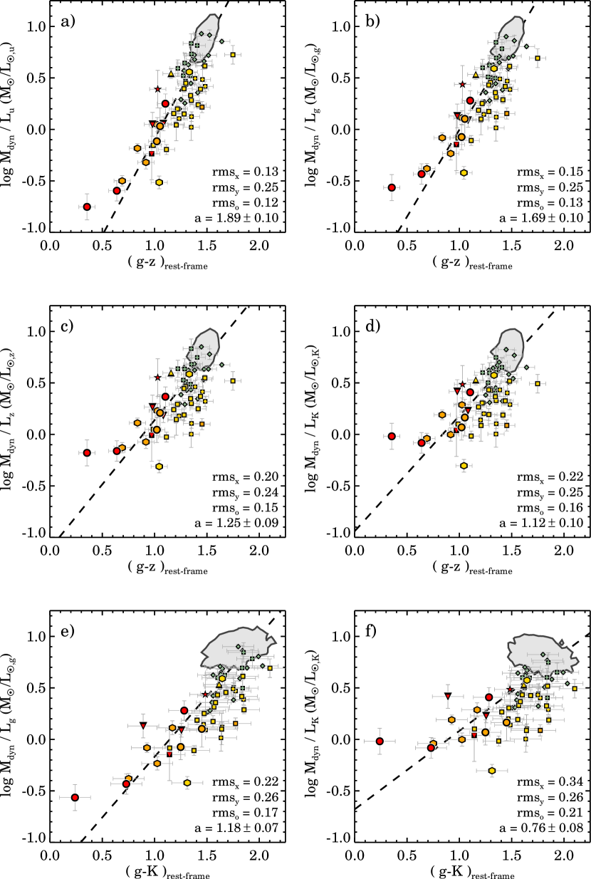
Figure 3.— $M/L$ vs. rest-frame color for massive galaxies between $z=0$ and $z=2$ for different luminosity bands and rest-frame colors. Symbols are similar as in Figure 1, and color coded by redshift. From the rest-frame $u$ to the $K$ band, there is a large range in the $M/L$: 1.8 dex in rest-frame $M/L_{\rm u}$, 1.6 dex in $M/L_{\rm g}$, and 1.3 dex in $M/L_{\rm K}$. We find a strong correlation between the $M/L$ for different luminosity bands and the rest-frame $g-z$ color. The $M_{\rm{dyn}}/L_{\rm u}$ versus $(g-z)_{\rm rest-frame}$ show the least amount of scatter. We use a linear fit to the data to describe the relation between the $M/L$ and rest-frame color, in which galaxies from the SDSS (gray contour) are given equal weight as the high-redshift data. The best-fit values are summarized in Table LABEL:tab:tab3 & LABEL:tab:tab4. For each fit we furthermore give the rms scatter orthogonal to the best-fitting line. Overall, the $M_{\rm{dyn}}/L_{\rm g}$ vs $g-z$ color gives little scatter (rms${}_{o}\sim 0.12$ dex), whereas the scatter is higher when we use the rest-frame $g-K$ color (rms${}_{o}\sim 0.17$ dex).

Figure 4.— Slope $a_{\rm\lambda}$ from the $M/L_{\rm\lambda}$ vs. $(g-z)_{\rm rest-frame}$ relation versus wavelength $\lambda$. For each luminosity band, we use the values from Table LABEL:tab:tab3, and the errors are derived from bootstrapping the data. In the rest-frame $u$ band, we find a steep slope of $\sim 2.0$. The slope $a_{\rm\lambda}$ decreases when we go from the $u$ to $i$ band. Redwards of the $z$ band, we find that the relation between the $M/L$ vs. $g-z$ color is approximately $\sim 1.2$.

Table 3Emperical Relations for the $M/L$ vs. rest-frame Color using SDSS filters

color	$a_{\rm u}$	$b_{\rm u}$	rmsu	$a_{\rm g}$	$b_{\rm g}$	rmsg	$a_{\rm r}$	$b_{\rm r}$	rmsr	$a_{\rm i}$	$b_{\rm i}$	rmsi	$a_{\rm z}$	$b_{\rm z}$	rmsz	$a_{\rm J}$	$b_{\rm J}$	rmsJ	$a_{\rm H}$	$b_{\rm H}$	rmsH	$a_{\rm K}$	$b_{\rm K}$	rmsK
$u-g$	5.02	-7.35	0.08	4.77	-6.95	0.08	4.31	-6.21	0.09	4.08	-5.85	0.09	4.10	-5.91	0.09	4.07	-5.89	0.09	4.19	-6.08	0.10	4.04	-5.81	0.10
$u-r$	1.93	-3.92	0.12	1.72	-3.42	0.13	1.48	-2.86	0.14	1.36	-2.58	0.15	1.29	-2.45	0.15	1.26	-2.38	0.16	1.22	-2.29	0.16	1.16	-2.14	0.16
$u-i$	1.47	-3.31	0.33	1.31	-2.87	0.31	1.13	-2.39	0.30	1.04	-2.15	0.30	0.98	-2.03	0.29	0.96	-1.99	0.28	0.93	-1.92	0.28	0.89	-1.78	0.28
$u-z$	1.28	-3.18	0.66	1.14	-2.76	0.61	0.99	-2.29	0.58	0.91	-2.05	0.56	0.85	-1.93	0.55	0.83	-1.87	0.53	0.81	-1.82	0.53	0.77	-1.68	0.53
$u-J$	1.09	-3.00	1.08	0.97	-2.58	1.02	0.83	-2.11	0.97	0.76	-1.88	0.94	0.71	-1.75	0.92	0.67	-1.65	0.90	0.65	-1.60	0.90	0.62	-1.47	0.89
$u-H$	1.04	-3.04	1.30	0.93	-2.62	1.23	0.80	-2.17	1.16	0.73	-1.93	1.13	0.69	-1.81	1.11	0.65	-1.70	1.09	0.63	-1.64	1.08	0.60	-1.51	1.07
$u-K$	0.99	-2.61	0.96	0.88	-2.26	0.92	0.76	-1.85	0.88	0.70	-1.65	0.86	0.66	-1.55	0.84	0.63	-1.48	0.83	0.61	-1.42	0.83	0.57	-1.28	0.82
$g-r$	4.06	-2.47	0.07	3.73	-2.22	0.08	3.46	-2.01	0.09	3.24	-1.83	0.09	3.24	-1.86	0.09	3.30	-1.93	0.10	3.22	-1.87	0.10	3.14	-1.80	0.10
$g-i$	2.62	-2.22	0.10	2.41	-1.99	0.11	1.92	-1.46	0.12	1.75	-1.27	0.13	1.65	-1.19	0.13	1.61	-1.16	0.14	1.56	-1.12	0.14	1.47	-1.00	0.14
$g-z$	1.89	-1.97	0.12	1.69	-1.69	0.13	1.45	-1.36	0.14	1.32	-1.18	0.15	1.25	-1.11	0.15	1.21	-1.08	0.16	1.18	-1.04	0.16	1.12	-0.94	0.16
$g-J$	1.54	-2.03	0.16	1.37	-1.74	0.16	1.18	-1.40	0.17	1.07	-1.21	0.18	1.00	-1.12	0.19	0.95	-1.05	0.20	0.92	-1.01	0.20	0.87	-0.91	0.20
$g-H$	1.46	-2.18	0.16	1.31	-1.88	0.17	1.13	-1.52	0.18	1.03	-1.34	0.18	0.97	-1.24	0.19	0.92	-1.17	0.20	0.89	-1.12	0.20	0.84	-1.01	0.20
$g-K$	1.31	-1.57	0.17	1.18	-1.35	0.17	1.02	-1.07	0.18	0.93	-0.93	0.18	0.88	-0.87	0.19	0.84	-0.83	0.20	0.82	-0.79	0.20	0.76	-0.68	0.21
$r-i$	7.33	-1.71	0.04	7.05	-1.63	0.04	6.66	-1.50	0.05	6.42	-1.42	0.05	6.41	-1.44	0.05	5.91	-1.29	0.05	6.18	-1.40	0.05	6.11	-1.36	0.05
$r-z$	4.87	-2.34	0.06	4.52	-2.11	0.07	4.30	-1.96	0.07	4.00	-1.80	0.08	3.95	-1.80	0.08	4.13	-1.91	0.09	4.12	-1.91	0.09	3.87	-1.74	0.09
$r-J$	2.57	-1.85	0.13	2.28	-1.56	0.13	1.93	-1.22	0.14	1.75	-1.05	0.15	1.60	-0.93	0.16	1.48	-0.83	0.17	1.43	-0.79	0.17	1.35	-0.69	0.18
$r-H$	2.34	-2.06	0.13	2.07	-1.74	0.14	1.75	-1.37	0.15	1.59	-1.19	0.15	1.48	-1.10	0.16	1.35	-0.97	0.17	1.30	-0.91	0.18	1.23	-0.81	0.18
$r-K$	1.99	-1.19	0.14	1.77	-0.99	0.15	1.53	-0.76	0.15	1.39	-0.64	0.16	1.29	-0.57	0.17	1.20	-0.51	0.18	1.16	-0.48	0.18	1.06	-0.37	0.19

Table 4Emperical Relations for the $M/L$ vs. rest-frame Color using Johnson-Cousin Filters

color	$a_{\rm U}$	$b_{\rm U}$	rmsU	$a_{\rm B}$	$b_{\rm B}$	rmsB	$a_{\rm V}$	$b_{\rm V}$	rmsV	$a_{\rm R}$	$b_{\rm R}$	rmsR	$a_{\rm I}$	$b_{\rm I}$	rmsI	$a_{\rm J}$	$b_{\rm J}$	rmsJ	$a_{\rm H}$	$b_{\rm H}$	rmsH	$a_{\rm K}$	$b_{\rm K}$	rmsK
$U-B$	10.16	-10.42	0.06	9.86	-10.04	0.06	9.44	-9.62	0.06	9.32	-9.49	0.06	8.63	-8.73	0.06	10.31	-10.63	0.07	9.39	-9.59	0.07	9.19	-9.38	0.07
$U-V$	2.44	-4.12	0.10	2.28	-3.77	0.11	1.97	-3.20	0.12	1.83	-2.94	0.13	1.68	-2.65	0.13	1.58	-2.50	0.14	1.55	-2.44	0.14	1.47	-2.27	0.14
$U-R$	1.77	-3.47	0.13	1.66	-3.18	0.13	1.44	-2.69	0.14	1.33	-2.46	0.15	1.22	-2.22	0.16	1.15	-2.08	0.17	1.12	-2.01	0.17	1.06	-1.86	0.17
$U-I$	1.39	-3.05	0.30	1.31	-2.79	0.29	1.13	-2.37	0.28	1.05	-2.15	0.28	0.96	-1.93	0.28	0.90	-1.81	0.27	0.88	-1.75	0.27	0.84	-1.62	0.27
$U-J$	1.08	-2.84	0.94	1.01	-2.58	0.91	0.87	-2.17	0.86	0.80	-1.95	0.84	0.73	-1.73	0.82	0.67	-1.56	0.79	0.65	-1.50	0.79	0.61	-1.38	0.78
$U-H$	1.04	-2.90	1.15	0.97	-2.63	1.12	0.84	-2.22	1.06	0.78	-2.01	1.03	0.71	-1.78	1.01	0.65	-1.61	0.97	0.63	-1.55	0.97	0.59	-1.42	0.96
$U-K$	0.98	-2.47	0.83	0.92	-2.25	0.81	0.80	-1.90	0.78	0.74	-1.72	0.76	0.68	-1.52	0.75	0.62	-1.39	0.72	0.61	-1.33	0.72	0.57	-1.19	0.71
$B-V$	3.95	-2.75	0.07	3.79	-2.59	0.07	3.44	-2.30	0.08	3.27	-2.17	0.09	3.11	-2.05	0.09	3.22	-2.17	0.10	3.13	-2.10	0.10	2.94	-1.91	0.10
$B-R$	2.55	-2.52	0.10	2.47	-2.38	0.10	2.15	-2.01	0.11	1.83	-1.63	0.12	1.66	-1.44	0.13	1.58	-1.36	0.14	1.54	-1.32	0.14	1.47	-1.21	0.14
$B-I$	1.72	-2.06	0.12	1.63	-1.88	0.13	1.42	-1.57	0.14	1.30	-1.41	0.15	1.20	-1.25	0.15	1.14	-1.19	0.16	1.11	-1.15	0.16	1.05	-1.05	0.17
$B-J$	1.32	-2.16	0.17	1.24	-1.96	0.17	1.07	-1.64	0.18	0.99	-1.47	0.18	0.90	-1.29	0.19	0.82	-1.16	0.21	0.80	-1.12	0.21	0.76	-1.01	0.21
$B-H$	1.26	-2.27	0.17	1.19	-2.07	0.17	1.03	-1.75	0.18	0.95	-1.57	0.19	0.87	-1.38	0.19	0.80	-1.26	0.21	0.77	-1.20	0.21	0.73	-1.09	0.21
$B-K$	1.14	-1.73	0.17	1.08	-1.56	0.18	0.94	-1.31	0.18	0.87	-1.17	0.19	0.79	-1.02	0.19	0.74	-0.94	0.21	0.71	-0.90	0.21	0.67	-0.79	0.21
$V-R$	7.86	-2.31	0.04	8.00	-2.31	0.04	7.29	-2.08	0.04	6.96	-1.95	0.05	6.57	-1.84	0.05	6.87	-1.98	0.05	6.73	-1.91	0.05	6.35	-1.76	0.05
$V-I$	3.89	-2.09	0.07	3.75	-1.95	0.07	3.45	-1.78	0.08	3.23	-1.63	0.08	3.15	-1.59	0.09	3.23	-1.68	0.10	3.12	-1.59	0.10	3.02	-1.52	0.10
$V-J$	1.97	-1.85	0.14	1.85	-1.66	0.15	1.59	-1.37	0.15	1.45	-1.21	0.16	1.31	-1.04	0.17	1.15	-0.87	0.19	1.11	-0.83	0.19	1.05	-0.73	0.19
$V-H$	1.88	-2.09	0.14	1.76	-1.88	0.15	1.52	-1.56	0.16	1.39	-1.39	0.16	1.27	-1.22	0.17	1.12	-1.04	0.19	1.08	-0.98	0.19	1.02	-0.87	0.19
$V-K$	1.63	-1.35	0.16	1.54	-1.20	0.16	1.34	-0.99	0.16	1.23	-0.87	0.17	1.13	-0.75	0.17	1.02	-0.66	0.19	0.99	-0.62	0.19	0.91	-0.51	0.20

3. Empirical Relation Between the $M/L$ and Color

3.1. Color and the $M/L$ Evolution

In Figure 2(a) and (c) we show the rest-frame $g-z$ color and $M_{\rm dyn}/L_{\rm g}$ as a function of redshift. We find a large range in $g-z$ color ($\sim 1$mag) and $\log_{10}M_{\rm dyn}/L_{\rm g}$ ($\sim 1.6$ dex). At $z>1$, massive galaxies are bluer and have lower $M/L$ as compared to low-redshift. In van de Sande et al. (2014) we showed that our high-redshift spectroscopic sample is biased toward young quiescent galaxies. While this bias complicated the analysis of the fundamental plane as presented in that work, here we take advantage of that same bias, as it enables us to study massive quiescent galaxies with a large range in stellar population properties.

We show $(g-z)_{\rm rest-frame}$ versus the dynamical mass in Figure 2(b). We find a weak trend between dynamical mass and color for low-redshift galaxies. At $z>1.5$ the lowest mass galaxies have the bluest colors. Figure 2(d) shows the $M_{\rm dyn}/L_{\rm{g}}$ versus the dynamical mass. For galaxies in the SDSS, there is a positive correlation such that low mass galaxies also have lower $M/L$ as compared to more massive galaxies. In the mass range of $10^{11}<M_{\rm dyn}/M_{\odot}<10^{12}$, the $M_{\rm dyn}/L_{\rm{g}}$ for galaxies in the SDSS increases by about $\sim 0.2~{}$dex. For galaxies at $z>0.5$ in our sample, we find that galaxies with high $M/L$ are on average more massive as compared to galaxies with low $M/L$.

3.2. Empirical Relation Between the $M/L$ and Color

Next, we examine empirical relations between the $M/L$ and color, as first predicted by Tinsley (1972; 1980). In Figure 3(a-d) we show the dynamical $M/L$ vs. rest-frame $g-z$ color in the following filters: $u$, $g$, $z$, and $K$. Figures 3(e) and (f) show the rest-frame $g-K$ colors versus the $M/L_{\rm g}$ and $M/L_{\rm K}$. Symbols are similar to Figure 2. Massive quiescent galaxies ($>10^{11}M_{\odot}$) from the SDSS are shown by the gray contour, which encloses $68\%$ of all galaxies. We find that the $\log_{10}M/L_{\rm u}$ varies most, from $\sim-0.7$ to $\sim 1.1$. The range in $\log_{10}M/L$ slowly decreases with increasing wavelength from $1.8$ dex in the $u$ band, to 1.6 dex in the $g$ band, and 1.3 dex in the $z$ and $K$ band.

As expected, we find a strong positive correlation between the $M/L$ in all passbands and rest-frame colors. Following Bell & de Jong (2001), we fit the simple relation:

$$\log_{10}M_{\rm dyn}~{}/~{}L_{\rm\lambda}=a_{\rm\lambda}*{color}~{}+~{}b_{\rm\lambda}$$ (3)

We use the IDL routine $LINMIX\_ERR$ which is a Bayesian method to measure the linear regression, with regression coefficients $a_{\rm\lambda}$ and $b_{\rm\lambda}$. The advantage of using a Bayesian approach over a routine that minimizes $\chi^{2}$, is that the Bayesian approach incorporates the intrinsic scatter as a fit parameter. In the fit we give equal weight to the SDSS galaxy sample and our sample of galaxies at intermediate to high redshift, instead of anchoring the fit to the median of the SDSS galaxies. In practice this means that we add 63 galaxies to the intermediate and high-z sample, which have a $M/L$ and color equal to the median of all SDSS galaxies. We note that when we use the IDL routine $FITEXY$, which minimizes the $\chi^{2}$ in the fit for both $x$ (rest-frame color) and $y$ ($M/L$), we find on average $\sim 5\%$ higher values for $a_{\rm\lambda}$. The results are summarized in Table LABEL:tab:tab3 using the SDSS filters and in Table LABEL:tab:tab4 where we use the Johnson-Cousin Filters.

Besides the coefficients, we also report the root-mean-square (rms_o) scatter, which is a good indicator for the significance of each relation. The scatter around the linear relation increases from 0.12 to 0.16 when going from rest-frame optical $M/L_{\rm u}$ to rest-frame near-infrared $M/L_{\rm K}$. Furthermore, we find that for the $M_{\rm dyn}/L_{\rm{g}}$ the scatter is lower when we use the rest-frame $g-z$ color as compared to the rest-frame $g-K$ color.

For the color $(g-z)_{\rm rest-frame}$ , we find that the slope of the relation becomes flatter from the UV to the near-infrared. To investigate this trend in more detail, we plot the slope $a_{\lambda}$ as a function of wavelength from the $M/L_{\rm\lambda}$ vs. $(g-z)_{\rm rest-frame}$ relation in Figure 4. We find that the slope becomes flatter when we go from the $u$ to $i$ waveband, while the slope is approximately constant ($\sim 1.2$) from $z$ to $K$.

These results indicate that the $M/L$ of an early-type galaxy can be predicted by a singe rest-frame color $g-z$ to an accuracy of $\sim 0.25$ dex. In particular the rest-frame $g-z$ color in combination with the rest-frame $g$ band luminosity, provides a good constrain for mass measurements of quiescent galaxies, as it has a large dynamic range in $M/L$ and color, in combination with little scatter around the linear relation.

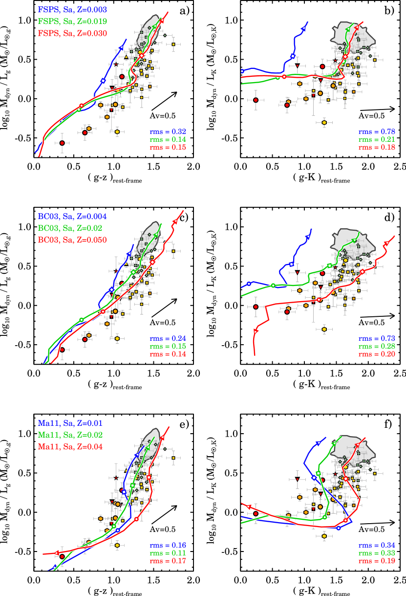
Figure 5.— $M/L$ vs. rest-frame color for the spectroscopic samples compared to the following SPS models: FSPS (top row), BC03 (middle row), and Ma11 (bottom row). The left column shows the $M_{\rm dyn}/L_{\rm{g}}$ vs. $(g-z)_{\rm rest-frame}$ , while the right column shows the $M_{\rm dyn}/L_{\rm{K}}$ vs. $(g-K)_{\rm rest-frame}$ . For each model we show three different metallicities: solar metallicity ($Z=0.02$, green), sub-solar metallicity (blue) and super-solar (red), and we indicate various model ages on the tracks with different symbols: 0.1 Gyr (upside down triangle), 1.0 Gyr (circle), 3.0 Gyr (diamond), 10 Gyr (triangle). The effect of dust is indicated by the black arrow. We find that none of the models are able to match both the rest-frame optical color and the rest-frame infrared color in combination with the $M/L$ simultaneously.

4. Comparisons with Stellar Population Synthesis Models

Here, we compare our dynamical $M/L$ vs. rest-frame color to the predictions from stellar population synthesis (SPS) models. Our main aim is to test whether the different SPS models can reproduce the relations in the optical and NIR and to what accuracy. For the comparison we use the SPS models by Bruzual & Charlot (2003; BC03), Maraston & Strömbäck (2011; Ma11), and Conroy & Gunn (2010) (FSPS, v2.4).

For the BC03 models we use the simple stellar population (SSP) models with the Padova stellar evolution tracks (Bertelli et al., 1994), and the STELIB stellar library (Le Borgne et al., 2003). For the Ma11 models, which are based on Maraston (2005; Ma05) with the Cassisi et al. (1997a), Cassisi et al. (1997b), and Cassisi et al. (2000) stellar evolution tracks and isochrones, we use SSPs with the red horizontal branch morphology and the MILES (Sánchez-Blázquez et al., 2006) stellar library. For the FSPS models, which use the latest Padova stellar evolution tracks (Marigo & Girardi 2007; Marigo et al. 2008), we use the standard program settings, and the MILES stellar library.

For all models we use a Salpeter (1955) IMF and a truncated SFH with a constant star formation rate for the first 0.5 Gyr. However, different SFHs result in nearly identical tracks. For example a longer star formation timescale will smooth out some of the small time-scale variations, but will not change any of our conclusions. For all models we use the total stellar mass, which is the sum of living stars and remnants. We note that our dynamical mass estimates include both stellar mass and dark matter mass. At this point we ignore the effect of dark matter, but we come back to this issue in Section 6.5.

In Figure 5 we compare the $M_{\rm dyn}/L_{\rm{g}}$ vs. $(g-z)_{\rm rest-frame}$ (left column) and $M_{\rm dyn}/L_{\rm{K}}$ vs. $(g-K)_{\rm rest-frame}$ (right column) with the predictions from SPS models. A different model is shown in each row from top to bottom: FSPS, BC03, and Ma11. For each model, we show three different metallicities: solar (green), sub-solar (blue) and super-solar (red). Metallicity values for the specific models are indicated in each panel. Furthermore, we indicate various model ages on the tracks with different symbols: 0.1 Gyr (upside down triangle), 1.0 Gyr (circle), 3.0 Gyr (diamond), 10 Gyr (triangle).

We indicate the effect of dust with the black arrow, assuming a Calzetti et al. (2000) dust law and $A_{\rm V}=0.5$. For the $M_{\rm dyn}/L_{\rm{g}}$ vs. rest-frame $g-z$ color, we find that the dust vector runs parallel to the model. Dust has, however, almost no affect on the rest-frame $K$ band luminosity and therefore runs nearly horizontal. To quantify how well the models match the data, we calculate the scatter orthogonal to the model tracks (rms_o). For the three models with different metallicities this scatter is given each panel in Figure 5 and in Table LABEL:tab:tab5. Below we discuss the comparison for SPS models individually.

4.1. FSPS models

In Figure 5(a) we show the $M_{\rm dyn}/L_{\rm{g}}$ vs. $(g-z)_{\rm rest-frame}$ color in combination with the FSPS models. The difference between the solar ($Z=0.02$) and super-solar ($Z=0.03$) tracks is small, whereas the sub-solar model is at all times too blue at fixed $M/L$. Both models with solar and super-solar metallicity match the $M_{\rm dyn}/L_{\rm{g}}$ and $(g-z)_{\rm rest-frame}$ color for low-redshift galaxies ($z<1$), but are unable to reproduce the low $M_{\rm dyn}/L_{\rm{g}}$ for the bluest galaxies with $(g-z)_{\rm rest-frame}$ $<1$. It is interesting to note that the scatter around the Solar metallicity model (0.14, Table LABEL:tab:tab5) is about similar to the scatter when assuming the linear fit (0.13, Figure 3(b)).

In Figure 5(b) we show the $M_{\rm dyn}/L_{\rm{K}}$ vs. the $(g-K)_{\rm rest-frame}$ color. The FSPS model tracks show a clear transition from a constant $M_{\rm dyn}/L_{\rm{K}}$ for $(g-K)_{\rm rest-frame}$ $<1.75$, to a very steep relation at $(g-K)_{\rm rest-frame}$ $>1.75$. The color difference between the solar ($Z=0.02$) and sub-solar ($Z=0.003$) tracks is large ($\Delta$$(g-z)_{\rm rest-frame}$ $\sim 0.8$) and more distinct as compared to the rest-frame $g-z$ color. The difference between solar and super-solar metallicity tracks is small for the FSPS models. The scatter for the Super-Solar metallicity model (0.18) is similar to the scatter for the linear fit (0.21, Figure 3(f)), even though the FSPS model track is far from linear. As in Figure 5(a), we find that both solar and super-solar tracks are able to match the low-redshift galaxies ($z<1$), but cannot simultaneously match the bluest galaxies with $(g-K)_{\rm rest-frame}$ $<1.5$ colors, for which the model $M/L$ is too high.

Table 5Scatter around SPS Models with different metallicities

SPS Model	$M/L$	color	Sub-Solar	Solar	Super-Solar
FSPS	$M/L_{\rm g}$	$g-z$	0.32	0.14	0.15
	$M/L_{\rm K}$	$g-K$	0.78	0.21	0.18
BC03	$M/L_{\rm g}$	$g-z$	0.24	0.15	0.14
	$M/L_{\rm K}$	$g-K$	0.73	0.28	0.20
Ma11	$M/L_{\rm g}$	$g-z$	0.16	0.11	0.17
	$M/L_{\rm K}$	$g-K$	0.34	0.33	0.19

4.2. BC03 models

For the BC03 models, the solar-metallicity track matches the low-redshift galaxies well for the rest-frame optical colors (Figure 5(c)), but the $M/L$ of the bluest galaxies is still overestimated by $\sim 0.2$ dex. The difference between the solar and super-solar metallicity tracks is larger than for the FSPS models, but this is mainly due to the fact that the BC03 super-solar metallicity ($Z=0.05$) track is significantly higher than the FSPS models ($Z=0.03$). For low-redshift galaxies in the SDSS, the super-solar ($Z=0.05$) model predicts a $M/L$ that is too low by $\sim 0.3$ dex, while the scatter for the $z>0.5$ data with the super-solar model (0.14) is almost the same as the scatter for the solar model (0.15). The sub-solar (Z=0.004) model shows colors that are too blue at fixed $M_{\rm dyn}/L_{\rm{g}}$ at all times.

In Figure 5(d), there is a larger color separation between the three metallicity tracks as compared to Figure 5(c). At fixed age the color difference in rest-frame $g-K$ is approximately twice as large as the color difference in the rest-frame $g-z$ color, indicating that the first color provides a better constraint for metallicity (see also Bell & de Jong 2001). Interestingly, the slope of the BC03 models remain almost linear for the rest-frame $g-K$ color, in contrast with the other two models. Neither solar nor super-solar tracks provide a good match to all the data, but the super-solar metallicity track has significantly lower scatter than the solar metallicity (super-solar=0.20 vs. solar = 0.28). While the solar metallicity model is unable to reproduce the low $M/L$ of the bluest galaxies, the super-solar metallicity model is unable to reproduce the color and the $M/L$ for SDSS galaxies.

4.3. Ma11 models

The Ma11 models are systematically different than the other models (Figure 5(e) and (f)). The Ma11 models exhibit an ”S-shaped” relation between the $M/L$ and rest-frame color, in particular for the $g-K$ colors. The trend in the Ma11 models is such that for blue colors there is a small increase in the $M/L$, whereas there is a steep nearly vertical upturn in the $M/L$ at late ages. It is interesting to note that the Ma11 solar metallicity track is able to match the $M/L$ and rest-frame $g-z$ color of all galaxies. Furthermore, the Ma11 model shows the lowest scatter as compared to the other models: rms = 0.11.

However, for the $(g-K)_{\rm rest-frame}$ color the sub-solar and solar metallicity tracks provide a poor match (Figure 5(f)). The $Z=0.02$ model has a sharp increase in the $M/L$ around $(g-K)_{\rm rest-frame}$ $\sim 1.4$, after which it is too blue by $\sim 0.5$ mag compared to the data. The super-solar metallicity model is able to match all galaxies at $z<1$, but around 1 Gyr the $M/L$ is too low by $\sim 0.2$ dex.

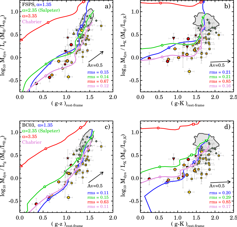
Figure 6.— $M/L$ vs. rest-frame color: comparing IMFs with different slopes. We use FSPS (top row) and BC03 (bottom row) models with solar metallicity ($Z=0.02$). The IMF is defined as a single power-law with slope $\alpha$. Different curves are IMFs with different realizations of $\alpha$. While the FSPS do not favor an IMF with $\alpha=1.35$ (blue) over $\alpha=2.35$ (green), the BC03 has less scatter for the IMF with $\alpha=1.35$ as compared to $\alpha=2.35$. Whereas a Chabrier IMF is able to reproduce the low $M/L$ for the bluest galaxies, it does not match the $M/L$ of low redshift SDSS galaxies in Panel (a) and (c). It does shows an excellent match to the data in Panel (b) and (d) with very little scatter.

4.4. Summary

All the models reproduce the general observed trend in $M/L$ vs. rest-frame color. Even though certain models with specific metallicity tracks match one $M/L$ vs. color, none of the models are able to simultaneously match the data in both the rest-frame $g-z$ vs. $M_{\rm dyn}/L_{\rm{g}}$ and $g-K$ vs. $M_{\rm dyn}/L_{\rm{K}}$ . In particular for FSPS and BC03, the models are unable to match the low $M/L$ for the bluest galaxies in combination with the rest of the data. For the $(g-z)_{\rm rest-frame}$ color, the Ma11 models are able to predict the low $M/L$ for the bluest galaxies at the same time as the $M/L$ for galaxies in the SDSS, with lower rms scatter as compared to the other models. We furthermore find that the SPS models exhibit different relations between the $M/L$ and rest-frame color, most prominently visible in the rest-frame $g-K$ color. The cause for the discrepancies between the models and the data, but also among the different models, can be due to several factors as there are a number of systematic differences in the SPS models. It is beyond the scope of this paper to address these differences, but we refer the reader to Conroy & Gunn (2010) for a recent comparison of several popular models.

5. Constraints on the IMF

In the previous Section we found that the models reproduce the general observed trend between $M/L$ and color, but cannot match all the data. Adapting a different IMF could provide a solution to this problem. The IMF influences the evolution and scaling of the $M/L$, while it has a smaller effect on the color evolution (Tinsley 1972; 1980). Generally speaking, a bottom-heavy IMF ($\alpha>2.35$) will give a flatter $M/L$ vs. color relation as compared to a bottom-light IMF ($\alpha<2.35$). In this Section, we explore the effect of the IMF on the different SPS models in the $M/L$ vs. color plane.

Table 6Scatter around SPS Models with different realizations of the IMF

SPS Model	$M/L$	color	x=1.35	x=2.35	x=3.35	Chabrier
FSPS	$M/L_{\rm g}$	$g-z$	0.15	0.14	0.67	0.12
	$M/L_{\rm K}$	$g-K$	0.21	0.21	0.85	0.15
BC03	$M/L_{\rm g}$	$g-z$	0.11	0.15	0.63	0.11
	$M/L_{\rm K}$	$g-K$	0.20	0.29	0.85	0.17

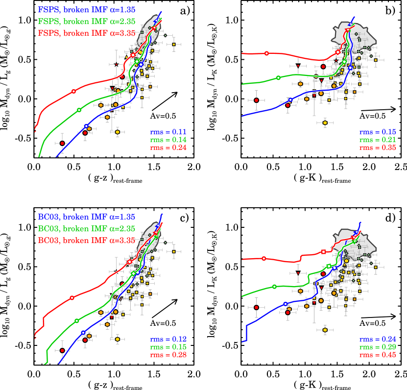
Figure 7.— $M/L$ vs. rest-frame color for an IMF with different slopes between 1$M_{\odot}~{}$and 4$M_{\odot}$. Below 1$M_{\odot}~{}$and above 4$M_{\odot}$, this IMF has a Salpeter slope, as defined according to Equation 5. We use FSPS (top row) and BC03 (bottom row) models with solar metallicity ($Z=0.02$). Based on the rms scatter, the models favor an IMF with a slope of $\alpha=1.35$ over $\alpha=2.35$. The FSPS model with a broken IMF of $\alpha=1.35$ is able to reproduce both the $M/L$ vs. $g-z$ and $g-K$ rest-frame color.

5.1. IMF Comparison

We show the FSPS (top row) and BC03 (bottom row) models with four different realizations of the IMF in Figure 6. We do not further explore the Ma11 models, because these models with different IMFs were not available to us. In this section we use solar metallicity models (FSPS $Z=0.0198$; BC03 $Z=0.02$), and a truncated SFH with a constant star formation rate for the first 0.5 Gyr. The Salpeter IMF with slope $\alpha=2.35$ is shown in green and was the assumed IMF in Figure 5. A bottom-light IMF with slope $\alpha=1.35$ is shown in blue, the bottom-heavy $\alpha=3.35$ IMF in red, and the Chabrier IMF in pink.

In Figure 6(a) we find that the FSPS model with the bottom-heavy IMF ($\alpha=3.35$) has a $M/L$ that is always too high and does not match any of the data. The steepest $M/L$ vs. color relation is predicted by the bottom-light IMF ($\alpha=1.35$). For the Salpeter and the bottom-light IMF we measure a similar rms scatter (0.14-0.15), but both IMFs have a $M/L$ that is on average too high by $\sim 0.1-0.2$ dex. The Chabrier IMF has a very similar behavior in the $M/L$ vs. color plane as the Salpeter IMF, but with a lower $M/L$ by about $\sim 0.2$ dex. For the bluest galaxies the Chabrier IMF reproduces the low $M/L$, but the $M/L$ is too low by $0.2$ dex for galaxies in the SDSS. Out of all four realizations of the IMF that we show in Figure 6(a), we measure the least scatter for the Chabrier IMF (0.12 dex).

For the $M_{\rm dyn}/L_{\rm{K}}$ vs. $(g-K)_{\rm rest-frame}$ (Figure 6(b)), we find similar differences between the IMFs as for the $M_{\rm dyn}/L_{\rm{K}}$ vs. $(g-z)_{\rm rest-frame}$ (Figure 6(a)). The bottom-heavy IMF ($\alpha=3.35$) overpredicts the $M/L$ by more than a dex and does not match any of the data. Compared to the Salpeter IMF, we find that the bottom-light IMF has a steeper $M/L$ vs. color relation, with a steep vertical upturn around 3 Gyr. Interestingly, the Chabrier IMF is able to match all data with very little scatter (0.15 dex).

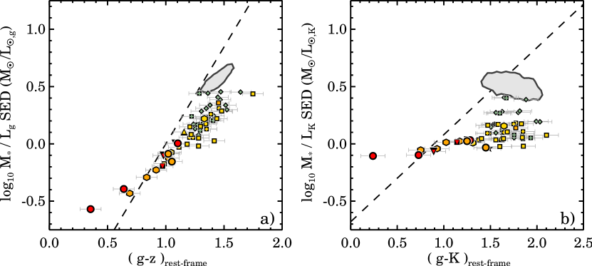
Figure 8.— $M_{*}/L$ versus rest-frame color. Here the $M/L$ have been determined by fitting solar metallicity BC03 models to the full broad-band data. Panel a) The galaxies lie along a tight sequence, but the relation is shallower as compared to the best-fit dynamical relation (dashed-line) from Section 3.2. Panel b) the SED derived $M_{*}/L_{\rm K}$ show a rather complex trend with $(g-K)_{\rm rest-frame}$ color similar to the trends for the FSPS and Ma11 models.

In Figure 6(c), we show the BC03 models with the four different realizations of the IMF. Again, the bottom-heavy IMF does not match any of the data. The bottom-light and Chabrier IMF both provide an excellent match to the intermediate and high-redshift data with the least rms scatter (0.11 dex). However, the Chabrier IMF again predicts a $M/L$ that is slightly too low for the SDSS sample.

The bottom-light IMF which gave a perfect match for the $M_{\rm dyn}/L_{\rm{g}}$ vs. $(g-z)_{\rm rest-frame}$, however, does not provide a good match for the intermediate galaxies in the $M_{\rm dyn}/L_{\rm{K}}$ vs. rest-frame $g-K$ color plane (Figure 6(d)). At $\mbox{$(g-K)_{\rm rest-frame}$}>1.4$ the $M/L$ of the bottom-light IMF is on average too high by $\sim 0.2$ dex. The bottom-light IMF still provides a better prediction than the Salpeter IMF with a respective rms of 0.20 vs 0.29. Again, we find that the Chabrier IMF best matches all the data based on the rms scatter (0.17), but does not provide a perfect match either.

Table 7Scatter around SPS Models with different realizations of the broken IMF

SPS Model	$M/L$	color	x=1.35	x=2.35	x=3.35
FSPS	$M/L_{\rm g}$	$g-z$	0.11	0.14	0.24
	$M/L_{\rm K}$	$g-K$	0.15	0.21	0.35
BC03	$M/L_{\rm g}$	$g-z$	0.12	0.15	0.28
	$M/L_{\rm K}$	$g-K$	0.24	0.29	0.45

Overall, we find that the BC03 model favors an IMF with a slope of $\alpha=1.35$ over an IMF with $\alpha=2.35$, while for the FSPS models we find no statistical preference for one of the two. We get an excellent match to the data with the FSPS model when using a Chabrier IMF for the rest-frame $g-K$ color, but for the rest-frame $g-z$ color this IMF underpredicts the $M/L$ for galaxies in the SDSS. As we still have not identified a model that can simultaneously match the $M/L$ vs. $(g-z)_{\rm rest-frame}$ and $(g-K)_{\rm rest-frame}$ colors, we explore a more exotic IMF in the next Section.

5.2. Broken IMF

As the $M/L$ vs. color relation is mostly sensitive to the IMF around the main sequence turnoff-point of stars in the Hertzsprung-Russell diagram, we experiment with a broken IMF, in which we only vary the slope between 1$M_{\odot}~{}$and 4$M_{\odot}$:

(5)

(6)

One advantage of this approach is that different realizations of the IMF will cause the SPS tracks to naturally intersect at late ages when most of the integrated light will come from low-mass stars with $M_{*}<1$$M_{\odot}$.

Figure 7 shows the three different realizations of the IMF using Equation 5: $\alpha=1.35$ (blue), $\alpha=2.35$ (green, normal Salpeter), and $\alpha=3.35$ (red). As before, we use solar metallicity models (FSPS $Z=0.0198$; BC03 $Z=0.02$), and a truncated SFH with a constant star formation rate for the first 0.5 Gyr.

As expected, in Figure 7(a) we find that the different tracks now all match the oldest $z\sim 0$ SDSS galaxies. This Figure also clearly shows that the $M/L$ vs. color relation becomes increasingly steep with decreasing slope of the IMF. We find that the FSPS model with $\alpha=1.35$ IMF is able to reproduce the low $M/L$ for the bluest galaxies and matches all the other data as well, with very little scatter (rms=0.11). Furthermore, the broken IMF with $\alpha=1.35$ provides a better match to the data than the IMF with slope $\alpha=2.35$. The bottom-heavy $\alpha=3.35$ IMF matches the highest $M/L$ galaxies, but for all galaxies bluer than $(g-z)_{\rm rest-frame}$ $<1.2$ the model $M/L$ is still too high. Most interestingly, in Figure 7(b) the FSPS model with $\alpha=1.35$ IMF matches all the data for the $M_{\rm dyn}/L_{\rm{K}}$ vs $(g-K)_{\rm rest-frame}$ with very little scatter (rms=0.15).

In Figure 7(c) we show the BC03 models with different realizations of the broken IMF. The broken IMF with $\alpha=1.35$ matches all the data from $z\sim 2$ to $z\sim 0$. However, for the $M_{\rm dyn}/L_{\rm{K}}$ vs. $(g-K)_{\rm rest-frame}$ color this IMF over-predicts the $M/L$ by $\sim 0.2$ dex (Figure 7(d)).

Therefore, based on the rms scatter, we conclude that both the FSPS and BC03 models favor a slope of the broken IMF of $\alpha=1.35$ over $\alpha=2.35$. We note that the FSPS model with a broken IMF of $\alpha=1.35$ is the only model that can reproduce both the $M/L$ vs. $g-z$ and $g-K$ rest-frame color.

6. Discussion and Comparison to Previous Studies

6.1. SED derived M/L

To investigate the implication of the results, we first compare our relation of $M_{\rm dyn}/L$ vs. rest-frame color to the relation of $(M_{*}/L)_{\rm SED}$ vs. rest-frame color. The $(M_{*}/L)_{\rm SED}$ has been determined by fitting solar metallicity BC03 models to the full photometric broad-band dataset (see Section 2.2). We show the results for our sample in Figure 8. In Figure 8(a) we compare the $(M_{*}/L_{\rm g})_{\rm SED}$ vs. rest-frame $g-z$ color with our best-fit dynamical relation from Section 3.2 (dashed line). As expected, the galaxies lie along a tight sequence. We note, however, that the best-fit dynamical relation is steeper. This difference in the steepness of the relation is consistent with the fact that the BC03 model tracks do not quite track the trends of Figure 5c. Figure 8(b) shows the $(M_{*}/L_{\rm K})_{\rm SED}$ versus $(g-K)_{\rm rest-frame}$. The derived $(M_{*}/L_{\rm K})_{\rm SED}$ show a rather complex trend with $(g-K)_{\rm rest-frame}$ color. This complex trend is similar to the trends for the FSPS (Figure 5(b)) and Ma11 (Figure 5(f)) SPS models.

The mismatch between the $(M_{*}/L_{\rm g})_{\rm SED}$ (using the BC03 models which were used to fit the full photometric broad-band dataset) and the $M_{\rm dyn}/L_{\rm{g}}$ is highlighted in Figure 9, where we compare the two estimates directly. In the case that the dynamical $M/L$ corresponds well to the SED based $M/L$, we expect to see a one-to-one linear relation (dashed line) with potentially a constant offset due to dark matter or low-mass stars. However, Figure 9 shows a relation that has a shallower slope than the dashed-line, such that galaxies with a lower $M/L$ are further offset from the one-to-one relation. This non-constant offset is similar to the results by van de Sande et al. (2013), in which we showed that $M_{*}/M_{\rm dyn}$ changes slightly as a function of redshift, where the $z\sim 2$ galaxies had the highest $M_{*}/M_{\rm dyn}$. However, as redshift, color, and $M_{\rm dyn}/L$ are correlated in our sample (see Figure 2(a) and (c)), the $M_{*}/M_{\rm dyn}$ trend with redshift could also be caused by the non-constant offset in $(M_{*}/L_{\rm g})_{\rm SED}$ vs. $M_{\rm dyn}/L_{\rm{g}}$. Without additional information (e.g., high signal-to-noise spectroscopy) it is hard to establish whether the trend is driven by galaxy structure evolution/dark matter fraction evolution, IMF variations (Section 5), or discrepancies in SPS models.

6.2. Intrinsic scatter

From the $M_{\rm dyn}/L_{\rm{g}}$ vs $(g-z)_{\rm rest-frame}$ color relation, we find that we can predict the $M/L$ of a galaxy with an accuracy of $\sim 0.25$ dex. However, our dynamical $M/L$ estimates suffer from large (systematic) uncertainties. To quantify the intrinsic scatter in the relation, we calculate the fraction of the scatter induced by uncertainties in the size, and velocity dispersion measurements. As the formal errors on the rest-frame colors are small ($<0.01$ mag), the scatter will be dominated by errors in the dynamical mass. From Monte-Carlo simulations, we find that 0.11 dex of the 0.25 dex scatter can be explained by measurement uncertainties. Thus our intrinsic scatter in the $M_{\rm dyn}/L_{\rm{g}}$ vs. $(g-z)_{\rm rest-frame}$ relation is 0.22 dex. However, if the (systematic) errors on the rest-frame colors are larger, for example $\sim 0.1$ mag, the intrinsic scatter would be 0.14 dex. Furthermore, from the Bayesian linear fit we obtain an estimate for the intrinsic scatter of 0.15 dex for the $(g-z)_{\rm rest-frame}$ vs. $M_{\rm dyn}/L_{\rm{g}}$. The intrinsic scatter can be due to variations in the star formation histories, metallicities for galaxies at high and low redshift, or may be due to unknown sources of measurement errors.

We also consider the fact that a single color might not provide an accurate constraint and that the full broad-band SED fit yields a tighter relation. We use the SED derived stellar $M/L$ (see also Section 6.1) to estimate the scatter when using the full broad-band dataset. We find a mean ratio of $M_{*}/M_{\rm dyn}=-0.20$ with an rms scatter of 0.20 dex. This scatter of 0.20 dex suggests that a single color (which had a $M/L$ accuracy of 0.25 dex) only provides a slightly worse $M/L$ prediction as compared to full broad-band SED fitting.

6.3. Comparison to Literature

6.3.1 Single-burst SPS models

The evolution of the rest-frame K-band $M/L$ out to $z\sim 1$ was measured for the first time by van der Wel et al. (2006), for a sample with a small dynamic range of approximately $\sim 0.4$ dex in $M/L_{\rm K}$. They concluded that single-burst BC03 models with a Salpeter IMF were offset with respect to the data and that the Ma05 models with a Salpeter IMF provided the best match. While we come to a similar conclusion for the BC03 models, we still find a large offset between the data and the Maraston models with a Salpeter IMF, as the Maraston solar metallicity tracks are too blue by 0.5 mag in rest-frame $g-K$. The different conclusion can be explained by the fact that van der Wel et al. (2006) used relative $M/L$ and colors, while we only use absolute values. We could not find other direct comparisons between $M_{\rm dyn}/L$ vs. color relations and SPS models in the literature.

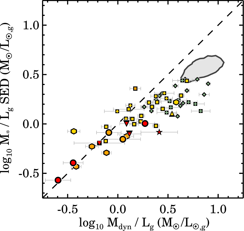
Figure 9.— $M_{*}/L_{\rm g}$ from SED fits vs. the $M_{\rm dyn}/L_{\rm{g}}$. The $M/L$ have been determined by fitting solar metallicity BC03 models to the full broad-band data. We find a non-linear relation, which could be due to an evolving dark matter fraction or IMF variations.

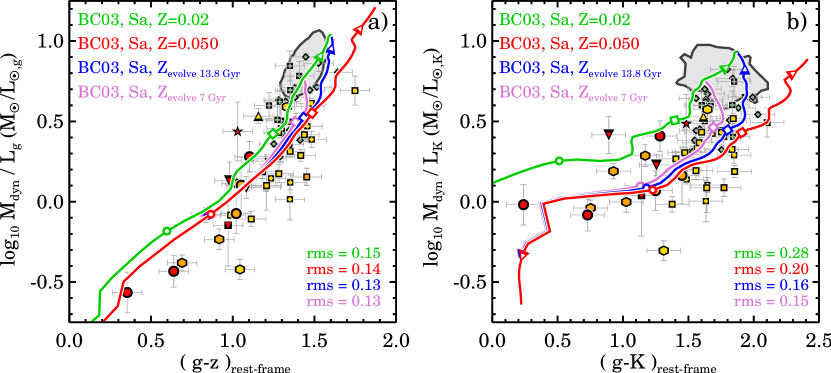
Figure 10.— $M/L$ vs. rest-frame color for evolving metallicities with BC03 models. The green ($Z=0.02$ and red ($Z=0.05$) model track are the same as in Figure 5(c) and (d). The blue track is a model where the metallicity evolves from $Z=0.05$ to $Z=0.02$ a function of time, over a period of 13.8 Gyr. The pink is similar to the blue track, but for this model the metallicity evolves from from $Z=0.05$ to $Z=0.02$ within the first 7 Gyr. The models with evolving metallicity show a slightly steeper relation as compared to the models without evolution in the metallicity.

6.3.2 Star-Forming Galaxies and extended SFH

The relation between $M/L$ vs. color was first explored by Bell & de Jong (2001) for spiral galaxies. They used an early version of the BC03 models, and found that the rest-frame $B-R$ color provided a good estimate of the $M/L$. Follow up work by Bell et al. (2003) used the Pegase SPS models with more extended SFHs to estimate SED based $M/L$, which were then used to derive observationally-constrained $M/L$ vs. color relations. They found that the optical $M/L$ vs. color relations were in good agreement with Bell & de Jong (2001), but they found a shallower slope in the NIR $M/L$ vs. color relation due to unaccounted metallicity effects. Zibetti et al. (2009) used the latest SPS models from Charlot & Bruzual (in Prep.) to directly derive the $M/L$ vs. color relation. Similar to the results by Gallazzi & Bell (2009) they found a steeper slope in the $M/L_{\rm i}$ vs. $(g-i)_{\rm rest-frame}$ relation as compared to Bell et al. (2003). Using BC03 models Taylor et al. (2011) follow a similar method as Bell et al. (2003) and found that slope for the $M/L_{\rm i}$ vs. $(g-i)$ relation is steeper than in Bell et al. (2003), but shallower than in Zibetti et al. (2009). Into & Portinari (2013) use the latest Padova isochrones, with detailed modelling of the Thermally Pulsing Asymptotic Giant Branch phase, to update the theoretical $M/L$-color relations. They also find a steeper slope for their new relations as compared to Bell et al. (2003).

In this Paper, we found that the slope for the $M/L_{\rm i}$ vs. rest-frame $(g-i)$ relation is considerably steeper than in previous work (e.g, Bell et al. 2003; Zibetti et al. 2009; Taylor et al. 2011; Into & Portinari 2013). The difference is easily explained as the $M/L$ vs. color relations in previous studies were derived from samples that include star-forming galaxies, with variable (exponentially declining) star formation histories, and dust. This naturally leads to a shallower slope. In addition, we found in Section 4 that most model tracks predict a shallower relation as compared to our dynamical data. If this trend is indeed caused by stellar population effects, it would imply that the masses of star forming galaxies need recalibration, and may have systematic uncertainties at a level of 0.2 dex.

6.4. Constraints on the IMF

Several authors have constrained the IMF’s using a differential analysis of color evolution against $M/L$ evolution, inspired by early work by Tinsley (1972; 1980). van Dokkum (2008a) used galaxies in clusters at $0<z<0.8$ and found an IMF slope around $1M_{\odot}$ of $\alpha=0.7^{+0.4}_{-0.7}$. Holden et al. (2010) used a larger sample, and analyzed the evolution at fixed velocity dispersion, and found an IMF slope of $\alpha=1.9\pm 0.2$. van Dokkum & Conroy (2012) repeated this analysis with the latest population models (Conroy & van Dokkum, 2012) and found a slope of $\alpha=1.81\pm 0.27$. Although the techniques used by these authors are quite different, the results are similar to those presented here. However, with our larger range in $M/L$ and rest-frame color, we find that the variations between different models with the same IMF are comparable to the variations due to the IMF with the same model. Therefore, with the current models it is still hard to put a robust constraint on the IMF.

6.5. Dark Matter

In this Paper we use dynamical mass estimates for calculating the $M/L$. The dynamical mass includes both stellar mass and dark matter mass, but to this point we have ignored the contribution of dark matter to the dynamical mass. At low-redshift the dynamical to stellar mass fraction is approximately a factor of $~{}1.6$ within one effective radius, due to the contribution of dark matter to the total mass. If we include dark matter in the $M/L$ of the models, this fraction would shift all curves in Figure 5-7 vertically up by $\sim 0.2$ dex. This shift would not solve the discrepancies between the models and the data, because the discrepancies are in the slope and cannot be solved by a constant offset (see Figure 9).

However, whether the dark matter fraction within one $r_{\rm e}$ is constant over time is still subject to debate. The size growth of massive quiescent galaxies may result in an increase of the dark matter to stellar mass fraction within one $r_{\rm e}$, because the dark matter profile is less steep than the stellar mass profile (see also Hilz et al. 2013). Thus, the dark matter fraction within one $r_{\rm e}$ may increase over time. In van de Sande et al. (2013), we indeed find a hint of an evolving dark matter fraction, i.e, the median $M_{*}/M_{dyn}$ is higher by $50\%$ at $z>1.5$ compared to massive SDSS galaxies ($M_{*}/M_{dyn}\propto(1+z)^{0.17\pm 0.011}$). From hydrodynamical simulations, Hopkins et al. (2009) find that for galaxies with $M_{*}\sim 10^{11}$, the stellar to dynamical mass ($M_{*}/M_{dyn}$) at $z\sim 2$ is lower by 0.1 dex. Thus, if we correct for an evolving dark matter fraction the $M/L$ for high-redshift galaxies would decrease by approximately $0.1$ dex and for SDSS galaxies by about $0.2$ dex. As this correction decreases the slope of the empirical $M/L$ vs. color relation, it would make the slope of the data more consistent with a Chabrier ($\alpha=2.35$) IMF (see Figure 6).

6.6. Metallicity & Complex Star Formation Histories

In the comparison of the models with the data, we used model tracks with single metallicities. As galaxies grow in size and mass over time, for example through minor mergers, metallicity may also evolve as the satellite galaxies have lower metallicities (e.g., Gallazzi et al. 2005; 2014; Choi et al. 2014). The core will likely keep the same metallicity, while the metallicity in the outskirts may decrease (Greene et al. 2013; Montes et al. 2014). Also, due to our stellar mass selection limit of $10^{11}$$M_{\odot}$, the descendent of the $z=2$ galaxies will be more massive than our $z=0$ selected galaxies. Thus, the average metallicity of $z=0$ galaxies in our sample is likely lower than that of the $z=2$ galaxies.

We make two simple models for which the metallicity is allowed to evolve as function of time from supersolar ($Z=0.05$) to solar ($Z=0.02$). In Figure 10 we show the BC03 models, similar to Figure 5(c) and (d). In blue, we show the model track with a metallicity transition timescale of 13.8 Gyr. For the pink model track, we assume that the metallicity evolution occurred within the first 7 Gyr after the burst. In Figure 10(a) the metallicity evolution has very little effect as the $Z=0.02$ and $Z=0.05$ metallicity tracks are close together. The rms scatter is only slightly lower for the model tracks with metallicity evolution (rms = 0.13) as compared to normal metallicity tracks (rms = 0.14-0.15). In Figure 10(b), both metallicity evolution tracks (blue and pink) show a steep vertical upturn in the $M/L$ around 3 Gyr, which improves the match with the observed data. The rms scatter is significantly lower for the models where the metallicity is allowed to evolve (e.g., 0.15 vs. 0.20).

While the BC03 models with metallicity evolution provide a better match for the $M_{\rm dyn}/L_{\rm{K}}$ vs. $(g-K)_{\rm rest-frame}$ (Figure 10(b)), these models do not provide a significant improvement for the $M_{\rm dyn}/L_{\rm{g}}$ vs. $(g-z)_{\rm rest-frame}$ , in particular at blue colors and low $M/L$. Without additional data (e.g., resolved images and spectroscopy) we cannot further quantify the effect of metallicity evolution.

Finally, we have assumed a single SFH for all galaxies. While massive galaxies in general are thought to have simple SFHs, for individual galaxies the SFH could be far more complex due to merging events. The fact that we find that none of the SPS models with a Salpeter or Chabrier IMF are able to simultaneously match all the data for both the rest-frame optical and NIR data could imply that the effect of a complex SFH is more important than assumed here.

6.7. Systematic Sample Variations

While the approach of using a mass selected sample has provided us with many insights it is clear that for comparing the $M/L$ of galaxies at different redshifts, this static mass selection could introduce a bias. Recent studies find that several properties of massive quiescent galaxies may change over time: they were smaller than their present-day counterparts (e.g., Daddi et al. 2005; Trujillo et al. 2006; van Dokkum et al. 2008b; Franx et al. 2008; van der Wel et al. 2008; and numerous others), their stellar masses increase by a factor of $\sim 2$ from $z\sim 2$ to $z\sim 0$ (e.g., van Dokkum et al. 2010, Patel et al. 2013), and the effective velocity dispersion may also decrease (e.g., Oser et al. 2012; van de Sande et al. 2013). Thus, our samples and measurements at different redshifts may not be directly comparable.

A possible additional complication is progenitor bias (e.g., van Dokkum & Franx 1996; 2001): the number density of massive galaxies changes by a factor of $\sim 10$ from $z\sim 2$ to $z\sim 0$ (Muzzin et al., 2013b). Thus, a substantial fraction of the current day early-type galaxies were star-forming galaxies at $z\sim 2$ (see also van der Wel et al. 2009). If the properties of the descendants of these $z\sim 2$ star-forming galaxies are systematically different from the descendants of the quiescent galaxies at $z\sim 2$, the simple single burst SPS models which we used here may produce a biased result.

7. CONCLUSIONS

In this Paper, we have used a sample of massive galaxies ($M_{*}>10^{11}M_{\odot}$) out to $z\sim 2$ with stellar kinematic, structural, and photometric measurements. The primary goals of this Paper are to study the empirical relation between the dynamical $M/L$ and rest-frame color, assess the ability of SPS models to reproduce this relation, and study the effect of the IMF on the $M/L$ vs color relation.

We find that our sample spans a large range in $M/L$: 1.8 dex in rest-frame $\log M_{\rm{dyn}}/L_{\rm u}$, 1.6 dex in $\log M_{\rm{dyn}}/L_{\rm g}$, and 1.3 dex in $\log M_{\rm{dyn}}/L_{\rm K}$. As expected for a passively evolving stellar population, we find a strong correlation between the $M/L$ for different bands and rest-frame colors. For rest-frame optical colors, the correlation is well approximated by a linear relation, and we provide coefficients of the linear fits for a large number of $M/L$ vs. color correlations. The root-mean-square scatter in the $\log M_{\rm{dyn}}/L$ residuals is $\sim 0.25$ dex. Thus, these relations are ideal for estimating masses for quiescent galaxies with an accuracy of $\sim 0.25$ dex.

We compare a combination of two $M/L$ vs. rest-frame color relations with SPS models by Bruzual & Charlot (2003), Maraston & Strömbäck (2011), and Conroy et al. (2009). Under the assumption of a Salpeter initial mass function (IMF), none of the SPS models are able to simultaneously match the data in $M_{\rm{dyn}}/L_{\rm g}$ vs. $(g-z)_{\rm rest-frame}$ color and $M_{\rm{dyn}}/L_{\rm K}$ vs. $(g-K)_{\rm rest-frame}$ color.

By changing the IMF, we test whether we can obtain a better match between the models and the data. IMFs with different slopes are still unable to simultaneously match the low $M/L$ of the bluest galaxies in combination with the other data. While a Chabrier IMF underpredicts the $M/L$ for $z\sim 0$ SDSS galaxies in the $M_{\rm{dyn}}/L_{\rm g}$ vs. $(g-z)_{\rm rest-frame}$, it provides an excellent match to all other data.

We also explore a broken IMF with a Salpeter slope at $M<1$$M_{\odot}~{}$ and $M>4$$M_{\odot}$, and we find that the models favor a slope of $\alpha=1.35$ over $\alpha=2.35$ in the intermediate region, based on the rms scatter. This time, the FSPS solar metallicity model with an IMF slope of $\alpha=1.35$, is able to simultaneously match both the $M/L$ vs. $(g-z)_{\rm rest-frame}$ and $(g-K)_{\rm rest-frame}$ relations.

The combination of the $M/L$ and color is a powerful tool for studying the shape of the IMF near 1$M_{\odot}~{}$. However, this work shows that the variations between different SPS models are comparable to the variations induced by changing the IMF. There are several caveats which may change our data or models tracks, among which an evolving dark matter fraction, an evolving metallicity, complicated star formation histories, and an evolving mass-selection limit. More complete and higher resolution empirical stellar libraries, improved stellar evolution models, and larger spectroscopic samples at high-redshift, are needed to provide more accurate constraints on the IMF.

References

- Abazajian et al. (2009) Abazajian, K. N., Adelman-McCarthy, J. K., Agüeros, M. A., et al. 2009, ApJS, 182, 543
- Bell et al. (2003) Bell, E. F., McIntosh, D. H., Katz, N., & Weinberg, M. D. 2003, ApJS, 149, 289
- Bell & de Jong (2001) Bell, E. F., & de Jong, R. S. 2001, ApJ, 550, 212
- Belli et al. (2014b) Belli, S., Newman, A. B., Ellis, R. S., & Konidaris, N. P. 2014b, ApJ, 788, L29
- Belli et al. (2014a) Belli, S., Newman, A. B., & Ellis, R. S. 2014a, ApJ, 783, 117
- Bertelli et al. (1994) Bertelli, G., Bressan, A., Chiosi, C., Fagotto, F., & Nasi, E. 1994, A&AS, 106, 275
- Bezanson et al. (2013a) Bezanson, R., van Dokkum, P., van de Sande, J., Franx, M., & Kriek, M. 2013a, ApJ, 764, L8
- Bezanson et al. (2013) Bezanson, R., van Dokkum, P. G., van de Sande, J., et al. 2013, ApJ, 779, LL21
- Bezanson et al. (2011) Bezanson, R., van Dokkum, P. G., Franx, M., et al. 2011, ApJ, 737, L31
- Blakeslee et al. (2006) Blakeslee, J. P., Holden, B. P., Franx, M., et al. 2006, ApJ, 644, 30
- Blanc et al. (2008) Blanc, G. A., Lira, P., Barrientos, L. F., et al. 2008, ApJ, 681, 1099
- Blanton et al. (2005) Blanton, M. R., Schlegel, D. J., Strauss, M. A., et al. 2005, AJ, 129, 2562
- Brammer et al. (2008) Brammer, G. B., van Dokkum, P. G., & Coppi, P. 2008, ApJ, 686, 1503
- Brammer et al. (2012) Brammer, G. B., van Dokkum, P. G., Franx, M., et al. 2012, ApJS, 200, 13
- Brinchmann et al. (2004) Brinchmann, J., Charlot, S., White, S. D. M., et al. 2004, MNRAS, 351, 1151
- Bruzual & Charlot (2003) Bruzual, G., & Charlot, S. 2003, MNRAS, 344, 1000
- Bundy et al. (2006) Bundy, K., Ellis, R. S., Conselice, C. J., et al. 2006, ApJ, 651, 120
- Calzetti et al. (2000) Calzetti, D., Armus, L., Bohlin, R. C., et al. 2000, ApJ, 533, 682
- Cappellari et al. (2006) Cappellari, M., Bacon, R., Bureau, M., et al. 2006, MNRAS, 366, 1126
- Cassisi et al. (1997a) Cassisi, S., Castellani, M., & Castellani, V. 1997a, A&A, 317, 108
- Cassisi et al. (1997b) Cassisi, S., degl’Innocenti, S., & Salaris, M. 1997b, MNRAS, 290, 515
- Cassisi et al. (2000) Cassisi, S., Castellani, V., Ciarcelluti, P., Piotto, G., & Zoccali, M. 2000, MNRAS, 315, 679
- Chabrier (2003) Chabrier, G. 2003, PASP, 115, 763
- Choi et al. (2014) Choi, J., Conroy, C., Moustakas, J., et al. 2014, ApJ, 792, 95
- Conroy (2013) Conroy, C. 2013, ARA&A, 51, 393
- Conroy & van Dokkum (2012) Conroy, C., & van Dokkum, P. 2012, ApJ, 747, 69
- Conroy & Gunn (2010) Conroy, C., & Gunn, J. E. 2010, ApJ, 712, 833
- Conroy et al. (2009) Conroy, C., Gunn, J. E., & White, M. 2009, ApJ, 699, 486
- Courteau et al. (2014) Courteau, S., Cappellari, M., de Jong, R. S., et al. 2014, Reviews of Modern Physics, 86, 47
- Daddi et al. (2005) Daddi, E., et al. 2005, ApJ, 626, 680
- de Jong & Bell (2007) de Jong, R. S., & Bell, E. F. 2007, Island Universes - Structure and Evolution of Disk Galaxies, 107
- De Lucia & Blaizot (2007) De Lucia, G., & Blaizot, J. 2007, MNRAS, 375, 2
- Förster Schreiber et al. (2006) Förster Schreiber, N. M., Franx, M., Labbé, I., et al. 2006, AJ, 131, 1891
- Franx et al. (2008) Franx, M., van Dokkum, P. G., Schreiber, N. M. F., Wuyts, S., Labbé, I., & Toft, S. 2008, ApJ, 688, 770
- Gallazzi et al. (2014) Gallazzi, A., Bell, E. F., Zibetti, S., Brinchmann, J., & Kelson, D. D. 2014, ApJ, 788, 72
- Gallazzi & Bell (2009) Gallazzi, A., & Bell, E. F. 2009, ApJS, 185, 253
- Gallazzi et al. (2005) Gallazzi, A., Charlot, S., Brinchmann, J., White, S. D. M., & Tremonti, C. A. 2005, MNRAS, 362, 41
- Greene et al. (2013) Greene, J. E., Murphy, J. D., Graves, G. J., et al. 2013, ApJ, 776, 64
- Hilz et al. (2013) Hilz, M., Naab, T., & Ostriker, J. P. 2013, MNRAS, 429, 2924
- Holden et al. (2010) Holden, B. P., van der Wel, A., Kelson, D. D., Franx, M., & Illingworth, G. D. 2010, ApJ, 724, 714
- Hopkins et al. (2009) Hopkins, P. F., Hernquist, L., Cox, T. J., Keres, D., & Wuyts, S. 2009, ApJ, 691, 1424
- Ilbert et al. (2013) Ilbert, O., McCracken, H. J., Le Fèvre, O., et al. 2013, A&A, 556, A55
- Into & Portinari (2013) Into, T., & Portinari, L. 2013, MNRAS, 430, 2715
- Kauffmann et al. (2003) Kauffmann, G., Heckman, T. M., White, S. D. M., et al. 2003, MNRAS, 341, 54
- Kriek et al. (2009) Kriek, M., van Dokkum, P. G., Labbé, I., et al. 2009, ApJ, 700, 221
- Kriek et al. (2008) Kriek, M., van der Wel, A., van Dokkum, P. G., Franx, M., & Illingworth, G. D. 2008, ApJ, 682, 896
- Kuntschner et al. (2010) Kuntschner, H., Emsellem, E., Bacon, R., et al. 2010, MNRAS, 408, 97
- Le Borgne et al. (2003) Le Borgne, J.-F., Bruzual, G., Pelló, R., et al. 2003, A&A, 402, 433
- Maraston (2005) Maraston, C. 2005, MNRAS, 362, 799
- Maraston & Strömbäck (2011) Maraston, C., & Strömbäck, G. 2011, MNRAS, 418, 2785
- Marchesini et al. (2009) Marchesini, D., van Dokkum, P. G., Förster Schreiber, N. M., et al. 2009, ApJ, 701, 1765
- Marigo et al. (2008) Marigo, P., Girardi, L., Bressan, A., et al. 2008, A&A, 482, 883
- Marigo & Girardi (2007) Marigo, P., & Girardi, L. 2007, A&A, 469, 239
- McLean et al. (2012) McLean, I. S., Steidel, C. C., Epps, H. W., et al. 2012, Proc. SPIE, 8446
- Montes et al. (2014) Montes, M., Trujillo, I., Prieto, M. A., & Acosta-Pulido, J. A. 2014, MNRAS, 439, 990
- Muzzin et al. (2013b) Muzzin, A., Marchesini, D., Stefanon, M., et al. 2013b, ApJ, 777, 18
- Muzzin et al. (2013a) Muzzin, A., Marchesini, D., Stefanon, M., et al. 2013a, ApJS, 206, 8
- Newman et al. (2010) Newman, A. B., Ellis, R. S., Treu, T., & Bundy, K. 2010, ApJ, 717, L103
- Oser et al. (2012) Oser, L., Naab, T., Ostriker, J. P., & Johansson, P. H. 2012, ApJ, 744, 63
- Patel et al. (2013) Patel, S. G., van Dokkum, P. G., Franx, M., et al. 2013, ApJ, 766, 15
- Peng et al. (2010) Peng, C. Y., Ho, L. C., Impey, C. D., & Rix, H.-W. 2010, AJ, 139, 2097
- Onodera et al. (2012) Onodera, M., Renzini, A., Carollo, M., et al. 2012, ApJ, 755, 26
- Salpeter (1955) Salpeter, E. E. 1955, ApJ, 121, 161
- Sánchez-Blázquez et al. (2006) Sánchez-Blázquez, P., Peletier, R. F., Jiménez-Vicente, J., et al. 2006, MNRAS, 371, 703
- Simard et al. (2011) Simard, L., Mendel, J. T., Patton, D. R., Ellison, S. L., & McConnachie, A. W. 2011, ApJS, 196, 11
- Simard (1998) Simard, L. 1998, Astronomical Data Analysis Software and Systems VII, 145, 108
- Skelton et al. (2014) Skelton, R. E., Whitaker, K. E., Momcheva, I. G., et al. 2014, ApJS, 214, 24
- Szomoru et al. (2013) Szomoru, D., Franx, M., van Dokkum, P. G., et al. 2013, ApJ, 763, 73
- Taylor et al. (2011) Taylor, E. N., Hopkins, A. M., Baldry, I. K., et al. 2011, MNRAS, 418, 1587
- Taylor et al. (2010) Taylor, E. N., Franx, M., Brinchmann, J., van der Wel, A., & van Dokkum, P. G. 2010, ApJ, 722, 1
- Tinsley (1980) Tinsley, B. M. 1980, Fund. Cosmic Phys., 5, 287
- Tinsley (1972) Tinsley, B. M. 1972, ApJ, 178, 319
- Toft et al. (2012) Toft, S., Gallazzi, A., Zirm, A., et al. 2012, ApJ, 754, 3
- Tremonti et al. (2004) Tremonti, C. A., Heckman, T. M., Kauffmann, G., et al. 2004, ApJ, 613, 898
- Trujillo et al. (2006) Trujillo, I., et al. 2006, MNRAS, 373, L36
- van de Sande et al. (2014) van de Sande, J., Kriek, M., Franx, M., Bezanson, R., & van Dokkum, P. G. 2014, ApJ, 793, L31
- van de Sande et al. (2013) van de Sande, J., Kriek, M., Franx, M., et al. 2013, ApJ, 771, 85
- van de Sande et al. (2011) van de Sande, J., Kriek, M., Franx, M., et al. 2011, ApJ, 736, L9
- van der Wel et al. (2012) van der Wel, A., Bell, E. F., Häussler, B., et al. 2012, ApJS, 203, 24
- van der Wel et al. (2009) van der Wel, A., Bell, E. F., van den Bosch, F. C., Gallazzi, A., & Rix, H.-W. 2009, ApJ, 698, 1232
- van der Wel et al. (2008) van der Wel, A., Holden, B. P., Zirm, A. W., et al. 2008, ApJ, 688, 48
- van der Wel et al. (2006) van der Wel, A., Franx, M., van Dokkum, P. G., et al. 2006, ApJ, 636, L21
- van der Wel et al. (2005) van der Wel, A., Franx, M., van Dokkum, P. G., et al. 2005, ApJ, 631, 145
- van Dokkum & Conroy (2012) van Dokkum, P. G., & Conroy, C. 2012, ApJ, 760, 70
- van Dokkum et al. (2010) van Dokkum, P. G., et al. 2010, ApJ, 709, 1018
- van Dokkum et al. (2009) van Dokkum, P. G., Kriek, M., & Franx, M. 2009, Nature, 460, 717
- van Dokkum et al. (2008b) van Dokkum, P. G., et al. 2008b, ApJ, 677, L5
- van Dokkum (2008a) van Dokkum, P. G. 2008a, ApJ, 674, 29
- van Dokkum & Franx (2001) van Dokkum, P. G., & Franx, M. 2001, ApJ, 553, 90
- van Dokkum & Franx (1996) van Dokkum, P. G., & Franx, M. 1996, MNRAS, 281, 985
- Vernet et al. (2011) Vernet, J., Dekker, H., D’Odorico, S., et al. 2011, A&A, 536, A105
- Whitaker et al. (2011) Whitaker, K. E., Labbé, I., van Dokkum, P. G., et al. 2011, ApJ, 735, 86
- Williams et al. (2009) Williams, R. J., Quadri, R. F., Franx, M., van Dokkum, P., & Labbé, I. 2009, ApJ, 691, 1879
- Wuyts et al. (2007) Wuyts, S., Labbé, I., Franx, M., et al. 2007, ApJ, 655, 51
- Wuyts et al. (2004) Wuyts, S., van Dokkum, P. G., Kelson, D. D., Franx, M., & Illingworth, G. D. 2004, ApJ, 605, 677
- Zibetti et al. (2009) Zibetti, S., Charlot, S., & Rix, H.-W. 2009, MNRAS, 400, 1181