Magnetic end-states in a strongly-interacting one-dimensional topological Kondo insulator

Abstract

Topological Kondo insulators are strongly correlated materials, where itinerant electrons hybridize with localized spins giving rise to a topologically non-trivial band structure. Here we use non-perturbative bosonization and renormalization group techniques to study theoretically a one-dimensional topological Kondo insulator, described as a Kondo-Heisenberg model where the Heisenberg spin-1/2 chain is coupled to a Hubbard chain through a Kondo exchange interaction in the $p$-wave channel (i.e., a strongly correlated version of the prototypical Tamm-Schockley model). We derive and solve renormalization group equations at two-loop order in the Kondo parameter, and find that, at half-filling, the charge degrees of freedom in the Hubbard chain acquire a Mott gap, even in the case of a non-interacting conduction band (Hubbard parameter $U=0$). Furthermore, at low enough temperatures, the system maps onto a spin-1/2 ladder with local ferromagnetic interactions along the rungs, effectively locking the spin degrees of freedom into a spin-$1$ chain with frozen charge degrees of freedom. This structure behaves as a spin-1 Haldane chain, a prototypical interacting topological spin model, and features two magnetic spin-$1/2$ end states for chains with open boundary conditions. Our analysis allows to derive an insightful connection between topological Kondo insulators in one spatial dimension and the well-known physics of the Haldane chain, showing that the ground state of the former is qualitatively different from the predictions of the naïve mean-field theory.

I Introduction

Starting with the pioneering works of Kane and Mele Kane and Mele (2005a, b) and others Moore and Balents (2007); Roy (2009); Fu et al. (2007), there has been a surge of interest in topological characterization of insulating states Hasan and Kane (2010); Qi and Zhang (2011); Bernevig and Hughes (2013). It is now understood that there exist distinct symmetry-protected classes of non-interacting insulators, such that two representatives from different classes can not be adiabatically transformed into one another (without closing the insulating gap and breaking the underlying symmetry along the way). A complete topological classification of such band insulators has been developed in the form of a “periodic table of topological insulators” Kitaev (2009); Ryu et al. (2010). Furthermore, it was realized that the non-trivial (topological) insulators from this table possess, as their hallmark features, gapless boundary modes. The latter have been spectacularly observed in a variety of experiments in both three Hsieh et al. (2008); Xia et al. (2009) and two-dimensional systems König et al. (2007); Knez et al. (2011); Nowack et al. (2013); Spanton et al. (2014).

The aforementioned classification however is limited to non-interacting systems and as such it represents a classification of single-particle band structures. Adding interactions to the theory leads to significant complications. To understand and classify strongly-interacting topological insulator phases in many-particle systems is a fundamental open problem in condensed matter.

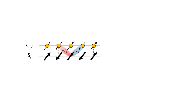
Figure 1: Schematic representation of the 1D “p-wave” Kondo-Heisenberg model. The top chain corresponds to the Hubbard model and the bottom chain is the $S=1/2$ antiferromagnetic Heisenberg model. The Kondo exchange (depicted pictorially as slanted bonds with odd inversion symmetry) is a non-local nearest-neighbor antiferromagnetic interaction $J_{K}>0$ which couples a spin $\mathbf{S}_{j}$ in the Heisenberg chain with the “p-wave” spin-density $\boldsymbol{\pi}_{j}$ in the Hubbard chain [see Eq. (4)].

A class of material that combines strong interactions and non-trivial topology of emergent bands are topological Kondo insulators (TKIs) Dzero et al. (2010). A basic model of these heavy fermion systems involves even-parity conduction electrons hybridizing with strongly correlated $f$-electrons. At low temperatures, a hybridization gap opens up and an insulating state can be formed. Its simplified mean-field description makes it amenable to a topological classification according to the non-interacting theory, and a topologically-non-trivial state appears due to the opposite parities of the states being hybridized. Although the mean-field description (formally well-controlled in the large-$N$ approximation Read and Newns (1983); Coleman (1987); Newns and Read (1987)) does appear to correctly describe the nature of the topological Kondo insulating states observed in bulk materials so far Reich (2012); Zhang et al. (2013); Kim et al. (2013); Wolgast et al. (2013); Neupane et al. (2013), it is interesting to see if non-perturbative effects beyond mean-field can qualitatively change the mean-field picture.

In contrast to higher dimensions, where reliable theoretical techniques to treat strong interactions are scarce, there exists a rich arsenal of such non-perturbative methods for one-dimensional systems, where strongly-correlated “non-mean-field” ground states abound. Since the Kondo insulating Hamiltonian and its mean-field treatment are largely dimension-independent, it is interesting to consider the one-dimensional such model as a natural playground to study interplay between strong interactions and non-trivial topology.

With this motivation in mind, we study here a strongly-interacting model of a one-dimensional topological Kondo insulator, i.e., a “$p$-wave” Kondo-Heisenberg model, introduced earlier by Alexandrov and Coleman Alexandrov and Coleman (2014), who treated the problem in the mean-field approximation. Here, we go beyond the mean-field level and consider quantum fluctuations non-peturbatively using the Abelian bosonization technique. It is shown that a “topological coupling” between the electrons in the Hubbard chain and spins in the Heisenberg chain, gives rise to a charge gap at half-filling in the former. The relevant interaction between the remaining spin-$1/2$ degrees of freedom in the chains is effectively ferromagnetic, which locks them into a state qualitatively similar to the Haldane’s spin-$1$ chain. The ground state therefore is a strongly-correlated topological insulator, which exhibits neutral spin-$1/2$ end modes.

While our main motivation is essentially theoretical (i.e., to allow a deeper understanding of strongly interacting topological matter), we believe our results might have direct application in ultracold atom experiments, where double-well optical superlattices loaded with atoms in $s$ and $p$ orbitals have been realized Wirth et al. (2011); Soltan-Panahi et al. (2012). In addition, our work might have some relevance in recent experimental results Nakajima et al. (2013); Eo et al. (2014); Fuhrman et al. (2014), which suggest the existence of a ferromagnetic phase transition and/or suppressed surface charge transport in samples of Samarium hexaboride ($\text{SmB}_{6}$ – a three-dimensional topological Kondo insulator).

This article is organized as follows: in Section II we specify the model for a 1D TKI and introduce the Abelian bosonization description. In Section III we present the renormalization group analysis and discuss the quantum phase diagram of the system. In Section IV we analyze the topological aspects of the problem and explain the emergence of topologically protected magnetic edge-states and in Section V we present a summary and discussion of results. Finally, in the Appendix A we present the technical derivation of the renormalization group equations.

II Model

We start our theoretical description by considering the Hamiltonian of the system depicted in Fig. 1, $H=H_{1}+H_{2}+H_{K}$ , where

$$H_{1} =-t\sum_{j=1,\sigma}^{N_{s}-1}\left(c_{j,\sigma}^{\dagger}c_{j+1,\sigma}+\mbox{H.c.}\right)-\mu\sum_{j=1,\sigma}^{N_{s}}n_{j,\sigma}$$

$$+U\sum_{j=1}^{N_{s}}\left(n_{j\uparrow}-\frac{1}{2}\right)\left(n_{j\downarrow}-\frac{1}{2}\right)$$ (1)

is a fermionic 1D Hubbard chain with $N_{s}$ sites, where $n_{j,\sigma}=c_{j,\sigma}^{\dagger}c_{j,\sigma}$ is the density of spin-$\sigma$ electrons at site $j$, $\mu$ is the chemical potential, and $U$ is the Hubbard interaction parameter. In this work we will only focus on the half-filled case $\mu=0$, where there is one electron per site. However, we expect our results to remain also valid for small deviations of half-filling. The spin chain is described by the spin-1/2 Heisenberg model

$$H_{2} =J\sum_{j=1}^{N_{s}-1}\mathbf{S}_{j}\cdot\mathbf{S}_{j+1},$$ (2)

with $J>0$. Here we assume the same lattice parameter $a$ for both chains $H_{1}$ and $H_{2}$. Finally, motivated by the work by Alexandrov and Coleman Alexandrov and Coleman (2014), we assume the following exchange coupling between the two chains

$$H_{K} =J_{K}\sum_{j=1}^{N_{s}}\mathbf{S}_{j}\cdot\boldsymbol{\pi}_{j},$$ (3)

where $J_{K}>0$ is the Kondo interaction between the $j-$th spin ($\mathbf{S}_{j}$) in the Heisenberg chain and the p-wave spin density in the fermionic chain at site $j$, defined as

$$\boldsymbol{\pi}_{j} \equiv p_{j,\alpha}^{\dagger}\left(\frac{\boldsymbol{\sigma}_{\alpha\beta}}{2}\right)p_{j,\beta},$$ (4)

where $p_{j,\alpha}\equiv\left(c_{j+1,\alpha}-c_{j-1,\alpha}\right)/\sqrt{2}$ is a linear combination of orbitals with $p$-wave symmetry, and $\boldsymbol{\sigma}_{\alpha\beta}$ is the vector of Pauli matrices. This model can be regarded as a strongly interacting version of the Tamm-Shockley model Tamm (1932); Shockley (1939); Pershoguba and Yakovenko (2012). While for our present purposes, this is an interesting “toy model” Hamiltonian that allows to extract a useful insight into strongly interacting topological phases, it could in principle be realized in ultracold-atom experiments [see Sec.V) for details]. In the absence of interactions in the fermionic chain (i.e., $U=0$) and in the large$-N$ mean-field approximation, Alexandrov and Coleman have shown the emergence of topologically-protected edge states arising from the non-trivial form of the Kondo term (3) Alexandrov and Coleman (2014). In their mean-field approach, the effective description of the system corresponds to non-interacting quasiparticles filling a strongly renormalized valence band with a non-trivial topology, stemming from the charge-conjugation, time-reversal and charge U(1) symmetry of the effectively non-interacting Hamiltonian (see also Ref. Li et al. (2013) for a discussion of a closely related system).

In this paper, our goal is to understand the emergence of topologically protected edge-states without introducing any decoupling of the Kondo interaction, including the interacting case, $U\neq 0$. We consider the case of small $U$ and $J_{K}$. This is formally represented by linearizing the non-interacting spectrum $\epsilon_{k}=-2t\cos ka$ in the fermionic chain $H_{1}$ around the Fermi energy $\mu=0$, and taking the continuum limit where the lattice constant $a\rightarrow 0$. Then, the fermionic operators admit the low-energy representation Giamarchi (2004); Gogolin et al. (1999a)

$$\frac{c_{j,\sigma}}{\sqrt{a}} \sim e^{ik_{F}x_{j}}R_{1,\sigma}\left(x_{j}\right)+e^{-ik_{F}x_{j}}L_{1,\sigma}\left(x_{j}\right),$$ (5)

where $R_{1,\sigma}\left(x\right)$ and $L_{1,\sigma}\left(x\right)$ are right and left moving fermionic field operators, which vary slowly on the scale of $a$. As we are interested in the edge-state physics, we consider open boundary conditions $c_{0,\sigma}=c_{N_{s}+1,\sigma}=0$, leading to the following constraints:

$$L_{1,\sigma}\left(0\right) =-R_{1,\sigma}\left(0\right),$$ (6)

$$L_{1,\sigma}\left(L_{c}\right) =-e^{i2k_{F}L_{c}}R_{1,\sigma}\left(L_{c}\right),$$ (7)

where $L_{c}=N_{s}a$ is the length of the chain. We next introduce the Abelian bosonization formalism Giamarchi (2004); Gogolin et al. (1999a)

$$R_{1,\sigma}\left(x\right) =\frac{F_{1,\sigma}}{\sqrt{2\pi\alpha}}e^{-i\phi_{1,R,\sigma}\left(x\right)},$$

$$L_{1,\sigma}\left(x\right) =\frac{F_{1,\sigma}}{\sqrt{2\pi\alpha}}e^{i\phi_{1,L,\sigma}\left(x\right)},$$ (8)

where $\alpha$ is a short distance cutoff in the bosonization procedure (we will take $\alpha=a$ hereafter). In Eq. (8) $\phi_{1,\lambda\sigma}\left(x\right)$ (with $\lambda=\left\{R,L\right\}$) are bosonic fields obeying the commutation relations $\left[\phi_{1,R\sigma}\left(x\right),\phi_{1,R\sigma^{\prime}}\left(y\right)\right]=i\pi\text{sign}\left(x-y\right)\delta_{\sigma,\sigma^{\prime}}$, $\left[\phi_{1,L\sigma}\left(x\right),\phi_{1,L\sigma^{\prime}}\left(y\right)\right]=-i\pi\text{sign}\left(x-y\right)\delta_{\sigma,\sigma^{\prime}}$, and $F_{1,\sigma}$ are Klein operators which obey anticommutation relations $\left\{F_{1,\sigma},F_{1,\sigma^{\prime}}\right\}=\delta_{\sigma,\sigma^{\prime}}$, and therefore ensure the correct anticommutation relations for fermions. Due to the constraints (6) and (7) introduced by the open boundary conditions, the right and left movers are not independent, and obey the constraints

$$\phi_{1,L,\sigma}\left(0\right) =-\phi_{1,R,\sigma}\left(0\right)+\pi,$$ (9)

$$\phi_{1,L,\sigma}\left(L_{c}\right) =-\phi_{1,R,\sigma}\left(L_{c}\right)+2k_{F}L_{c}-\pi+2q_{\sigma}\pi.$$ (10)

Here, $q_{\sigma}$ is an integer representing the occupation of the “zero-mode” excitations, i.e., particle-hole excitations with momentum $k=0$ and total spin $\sigma$. Its presence in Eq. (10) can be understood recalling that the expression of the non-chiral bosonic field $\phi_{1,\sigma}=\left(\phi_{1,R,\sigma}+\phi_{1,L,\sigma}\right)/2$ is Lecheminant and Orignac (2002)

$$\phi_{1,\sigma}\left(x\right) =\frac{\pi}{2}+\left(k_{F}L_{c}-\pi+\pi q_{\sigma}\right)\frac{x}{L_{c}}$$

$$+\sum_{n=1}^{\infty}\frac{\sin\left(k_{n}x\right)}{\sqrt{n}}\left(\alpha_{n,\sigma}+\alpha^{\dagger}_{n,\sigma}\right),$$

where $k_{n}\equiv\frac{\pi n}{L_{c}}$ with integer $n>0$, and $\alpha^{\dagger}_{n,\sigma}$ are bosonic operators obeying the commutation relation $\left[\alpha_{n,\sigma},\alpha^{\dagger}_{m,\sigma^{\prime}}\right]=\delta_{n,m}\delta_{\sigma,\sigma^{\prime}}$ (see Refs. von Delft and Schoeller, 1998; Lecheminant and Orignac, 2002 for details). From here we obtain the additional commutation relations Lecheminant and Orignac (2002)

$$\left[\phi_{1,R\sigma}\left(x\right),\phi_{1,L\sigma^{\prime}}\left(y\right)\right] =\begin{cases}-i\pi\delta_{\sigma,\sigma^{\prime}}&\text{for }0<x,y<L_{c},\\ 0&\text{for }x=y=0,\\ -2\pi i\delta_{\sigma,\sigma^{\prime}}&\text{for }x=y=L_{c}.\end{cases}$$ (11)

The bosonization procedure applied to the 1D Hubbard model is standard and we refer the reader to textbooks for details Giamarchi (2004); Gogolin et al. (1999a). Introducing charge and spin bosonic fields $\phi_{1,\lambda\sigma}=\frac{1}{\sqrt{2}}\left[\phi_{1c}-\lambda\theta_{1c}+\sigma\left(\phi_{1s}-\lambda\theta_{1s}\right)\right]$ (where the convention of signs $\lambda=\left\{R,L\right\}=\left\{+,-\right\}$ and $\sigma=\left\{\uparrow,\downarrow\right\}=\left\{+,-\right\}$ is implied), the 1D Hubbard model at half-filling (i.e., $k_{F}=\pi/2a$) becomes Giamarchi (2004)

$$H_{1} =\sum_{\nu=c,s}\int_{0}^{L_{c}}dx\;\left[\frac{v_{1\nu}}{2\pi K_{1\nu}}\left(\partial_{x}\phi_{1\nu}\right)^{2}+\frac{v_{1\nu}K_{1\nu}}{2\pi}\left(\partial_{x}\theta_{1\nu}\right)^{2}\right]$$

$$-\frac{U}{2\left(\pi a\right)^{2}}\int_{0}^{L_{c}}dx\;\left[\cos\left(\sqrt{8}\phi_{1c}\right)-\cos\left(\sqrt{8}\phi_{1s}\right)\right],$$ (12)

where the new fields obey the boundary conditions

$$\phi_{1s}\left(0\right)=0 ,\quad\phi_{1s}\left(L_{c}\right)=\frac{\pi}{\sqrt{2}}\left(q_{\uparrow}-q_{\downarrow}\right),$$ (13)

$$\phi_{1c}\left(0\right)=\frac{\pi}{\sqrt{2}} ,\quad\phi_{1c}\left(L_{c}\right)=\sqrt{2}\left(k_{F}L_{c}-\frac{\pi}{2}\right)+\frac{\pi}{\sqrt{2}}\left(q_{\uparrow}+q_{\downarrow}\right),$$ (14)

and the commutation relation $\left[\phi_{1,\nu}\left(x\right),\theta_{1,\nu^{\prime}}\left(y\right)\right]=-i\frac{\pi}{2}\delta_{\nu,\nu^{\prime}}\text{sign}\left(x-y\right)$. From here, we conclude that the field $\frac{1}{\pi}\partial_{x}\theta_{1,\nu}\left(x\right)$ is the momentum canonically conjugated to $\phi_{1,\nu}\left(x\right)$.

As is well-known, in 1D charge and spin excitations generally decouple and the above Hamiltonian can be split as $H_{1}=H_{1c}+H_{1s}$, with the first line describing independent Luttinger liquids for the charge and spin sectors, which are characterized by charge (spin) acoustic modes with velocities $v_{1c}=v_{F}\sqrt{1+Ua/\left(\pi v_{F}\right)}$ $\left(v_{1s}=v_{F}\right)$, and Luttinger parameter controlling the decay of correlation functions $K_{1c}=1/\sqrt{1+Ua/\left(\pi v_{F}\right)}$ ($K_{1s}=1$) . The presence of the cosine terms in the second line of (12) changes the physics qualitatively. In the present work, we restrict our focus to the case $U\geq 0$, where the term $\sim\cos\left(\sqrt{8}\phi_{1c}\right)$ is marginally relevant in the renormalization-group sense, and opens a Mott gap in the charge sector. At the same time, the term $\sim\cos\left(\sqrt{8}\phi_{1s}\right)$ is marginally irrelevant at the SU(2) symmetric point, and the spin sector remains gapless Gogolin et al. (1999a); Giamarchi (2004).

The bosonization of the Heisenberg chain $H_{2}$ is also quite standard and we refer the reader to the above-mentioned textbooks Giamarchi (2004); Gogolin et al. (1999a). A usual trick consists in representing the spin operators $\mathbf{S}_{j}$ by auxiliary fermionic operators in a half-filled Hubbard model with interaction parameter $U^{\prime}\gg U$. Therefore, while technically the procedure is identical to Eq. (12), the charge degrees of freedom in the bosonized Hamiltonian, $H_{2}$, can be assumed to be absent at the relevant energy scales of the problem due to the Mott gap $\sim U^{\prime}$. Then, ignoring the charge degrees of freedom and irrelevant operators in Eq. (12), and replacing the chain label $1\rightarrow 2$, we obtain

$$H_{2} =\frac{v_{2s}}{2\pi}\int_{0}^{L_{c}}dx\;\left[\left(\partial_{x}\phi_{2s}\right)^{2}+\left(\partial_{x}\theta_{2s}\right)^{2}\right].$$ (15)

Finally, we bosonize the Kondo Hamiltonian. The $p$-wave spin density in the fermionic chain and the spin density in the Heisenberg chain are, respectively

$$\frac{\boldsymbol{\pi}_{j}}{a} \sim 2\left[\mathbf{J}_{1R}\left(x_{j}\right)+\mathbf{J}_{1L}\left(x_{j}\right)-\left(-1\right)^{j}\mathbf{N}_{1}\left(x_{j}\right)\right],$$ (16)

$$\frac{\mathbf{S}_{j}}{a} \sim\mathbf{J}_{2R}\left(x_{j}\right)+\mathbf{J}_{2L}\left(x_{j}\right)+\left(-1\right)^{j}\mathbf{N}_{2}\left(x_{j}\right),$$ (17)

where $\mathbf{J}_{aR}\left(x\right)=R_{a,\alpha}^{\dagger}\left(x\right)\left(\frac{\boldsymbol{\sigma}_{\alpha,\beta}}{2}\right)R_{a,\beta}\left(x\right)$ and $\mathbf{J}_{aL}\left(x\right)=L_{a,\alpha}^{\dagger}\left(x\right)\left(\frac{\boldsymbol{\sigma}_{\alpha,\beta}}{2}\right)L_{a,\beta}\left(x\right)$ (with $a=1,2$) are the smooth components of the spin density, with bosonic representation

$$J_{a\lambda}^{x}\left(x\right) =\frac{1}{2\pi a}\cos\left\{\sqrt{2}\left[\lambda\phi_{a,s}\left(x\right)-\theta_{a,s}\left(x\right)\right]\right\},$$ (18)

$$J_{a\lambda}^{y}\left(x\right) =\frac{1}{2\pi a}\sin\left\{\sqrt{2}\left[\lambda\phi_{a,s}\left(x\right)-\theta_{a,s}\left(x\right)\right]\right\},$$ (19)

$$J_{a\lambda}^{z}\left(x\right) =-\frac{1}{\sqrt{8}\pi}\left[\partial_{x}\phi_{a,s}\left(x\right)-\lambda\partial_{x}\theta_{a,s}\left(x\right)\right],$$ (20)

where $\lambda=R(L)$ corresponds to the plus (minus) sign, and where $\mathbf{N}_{a}\left(x\right)=R_{a,\alpha}^{\dagger}\left(x\right)\left(\frac{\boldsymbol{\sigma}_{\alpha,\beta}}{2}\right)L_{a,\beta}\left(x\right)+\mbox{H.c.}$, are the staggered components

$$\mathbf{N}_{1}\left(x\right) =\frac{\cos\left[\sqrt{2}\phi_{1c}\left(x\right)\right]}{\pi a}\left(\cos\left[\sqrt{2}\theta_{1s}\left(x\right)\right],-\sin\left[\sqrt{2}\theta_{1s}\left(x\right)\right],-\cos\left[\sqrt{2}\phi_{1s}\left(x\right)\right]\right),$$ (21)

$$\mathbf{N}_{2}\left(x\right) =\frac{m_{2}}{\pi a}\left(\cos\left[\sqrt{2}\theta_{2s}\left(x\right)\right],-\sin\left[\sqrt{2}\theta_{2s}\left(x\right)\right],-\cos\left[\sqrt{2}\phi_{2s}\left(x\right)\right]\right),$$ (22)

with $m_{2}=\left\langle\cos\left[\sqrt{2}\phi_{2c}\left(x\right)\right]\right\rangle$ resulting from the integration of the gapped charge degrees of freedom in the Heisenberg chain. Therefore, although the spin densities (16) and (17) look similar in the bosonized language, they actually differ in two crucial aspects: 1) while in Eq. (22) the charge degrees of freedom are absent in the expression of the staggered magnetization, they are still present in (21) in the term $\cos\left(\sqrt{2}\phi_{1c}\left(x\right)\right)$ and we need to consider them. 2) Comparing Eqs. (16) and (17), we note a sign difference in the staggered components. This sign is related to the $p$-wave nature of the operators $p_{j,\sigma}$, and is therefore intimately connected to the topology of the Kondo interaction. The role of this sign turns out to be crucial in the rest of the paper.

Replacing the above results into Eq. (3), and taking the continuum limit, the Kondo interaction becomes in the bosonic language

$$H_{K} \sim 2J_{K}a\int_{0}^{L_{c}}dx\biggl{[}\sum_{\lambda,\lambda^{\prime}=L,R}:\mathbf{J}_{1\lambda}\left(x\right)\cdot\mathbf{J}_{2\lambda^{\prime}}\left(x\right):$$

$$-:\mathbf{N}_{1}\left(x\right)\cdot\mathbf{N}_{2}\left(x\right):\biggr{]},$$ (23)

where the sign in the second line is a consequence of the above mentioned sign in the staggered part of $\boldsymbol{\pi}\left(x\right)$.

Note that this model is reminiscent of the (non-topological) 1D Kondo-Heisenberg model, which has recently received much attention in the context of pair-density wave ordered phases in high-$T_{c}$ cuprate physics Zachar et al. (1996); Sikkema et al. (1997); Zachar and Tsvelik (2001); Zachar (2001); Berg et al. (2010); Dobry et al. (2013); Cho et al. (2014), and to the Hamiltonian of a spin-1/2 ladder Shelton et al. (1996); Gogolin et al. (1999b); Lecheminant and Orignac (2002); Robinson et al. (2012). However, a crucial difference with those works is the non-trivial structure of the Kondo interaction, which differs from the usual coupling $\sim J_{K}\mathbf{S}_{j}\cdot\mathbf{s}_{j}$, where $\mathbf{s}_{j}\equiv c_{j,\alpha}^{\dagger}\left(\frac{\boldsymbol{\sigma}_{\alpha\beta}}{2}\right)c_{j,\beta}$ is the standard (i.e., $s$-wave in this context) spin density in the fermionic chain. The first line in (23) is in fact closely related to the model considered in Refs. Sikkema et al. (1997); Zachar and Tsvelik (2001); Zachar (2001); Berg et al. (2010); Dobry et al. (2013). In the half-filling situation we are analyzing here, however, the most relevant part of $H_{K}$ (in the RG sense) is given by the product $\mathbf{N}_{1}\left(x\right)\cdot\mathbf{N}_{2}\left(x\right)$, which dominates the physics at low energies Shelton et al. (1996); Gogolin et al. (1999b); Lecheminant and Orignac (2002); Robinson et al. (2012). The term $\mathbf{N}_{1}\left(x\right)\cdot\mathbf{N}_{2}\left(x\right)$ only survives at half filling, and when both chains have the same lattice parameter (in other situations, the oscillatory factors $\leavevmode\nobreak\ e^{\pm i2k_{F}x}$ suppress this term, and the situation corresponds to the case analyzed in Refs. Sikkema et al. (1997); Zachar and Tsvelik (2001); Zachar (2001); Berg et al. (2010); Dobry et al. (2013)). Therefore, for our present purposes, we can neglect the first term in Eq. (23) and focus on the second term

$$H_{K} \approx-2J_{K}a\int_{0}^{L_{c}}dx\;\mathbf{N}_{1}\left(x\right)\cdot\mathbf{N}_{2}\left(x\right),$$

$$=-\frac{2J_{K}m_{2}}{\pi^{2}a}\int_{0}^{L_{c}}dx\;\cos\left(\sqrt{2}\phi_{1c}\right)$$

$$\left[\cos\left(\sqrt{2}\theta_{1s}\right)\cos\left(\sqrt{2}\theta_{2s}\right)+\sin\left(\sqrt{2}\theta_{1s}\right)\right.$$

$$\left.\times\sin\left(\sqrt{2}\theta_{2s}\right)+\sin\left(\sqrt{2}\phi_{1s}\right)\sin\left(\sqrt{2}\phi_{2s}\right)\right].$$ (24)

At this point we note that the problem is reminiscent of the well-known case of $S=1/2$ ladders with open boundary conditions Gogolin et al. (1999b); Lecheminant and Orignac (2002), with the important difference that here there is an extra factor $\sim\cos\left(\sqrt{2}\phi_{1c}\right)$.

The physics of the spin sector [i.e., term in square brackets in (24)] is quite non-trivial due to the presence of both the canonically conjugate fields $\phi_{a,s}\left(x\right)$ and $\theta_{a,s}\left(x\right)$, which cannot be simultaneously stabilized. However, the analysis of the charge sector is simpler, as only the field $\phi_{1c}\left(x\right)$ appears in the expression. This means that in the limit $J_{K}\rightarrow\infty$ the system can gain energy by “freezing out” the charge degrees of freedom, i.e., $m_{1}=\left\langle\cos\left[\sqrt{2}\phi_{1c}\left(x\right)\right]\right\rangle$, as there is no other competing mechanism. In the next Section we substantiate these ideas by providing a rigorous analysis.

III Renormalization-group analysis

Based on the similarity with the physics of spin ladders, we introduce symmetric and antisymmetric fields $\phi_{\pm}=\frac{1}{\sqrt{2}}\left(\phi_{1s}\pm\phi_{2s}\right)$ and $\theta_{\pm}=\frac{1}{\sqrt{2}}\left(\theta_{1s}\pm\theta_{2s}\right)$, in terms of which the Hamiltonian becomes

$$H_{K} =-\frac{J_{K}m_{2}}{\pi^{2}a}\int_{0}^{L_{c}}dx\;\cos\left(\sqrt{2}\phi_{1c}\right)$$

$$\times\left[-\cos\left(2\phi_{+}\right)+\cos\left(2\phi_{-}\right)+2\cos\left(2\theta_{-}\right)\right],$$ (25)

In what follows, we assume identical spinon dispersion $v_{1s}=v_{2s}=v_{s}$. Although this assumption is certainly an idealization, one can show that the asymmetry $\delta v\equiv v_{1s}-v_{2s}$ is an irrelevant perturbation in the renormalization-group sense, and therefore we do not expect that small asymmetries will have a qualitative effect on our results. We now write the Euclidean action of the system using complex space-time coordinates $z=v_{F}\tau+ix$ and $\overline{z}=v_{F}\tau-ix$, with $\tau=it$ the imaginary time, and the left and right fields $\phi_{\nu}=\left(\phi_{\nu L}+\phi_{\nu R}\right)/2$, where $\{\nu=+,-,1c\}$. The Euclidean action becomes:

$$S =S_{0}+S_{U}+S_{K},$$ (26)

$$S_{0} =-\frac{1}{4\pi}\int d^{2}r\Big{\{}\left(\partial_{z}\phi_{cL}\right)^{2}+\left(\partial_{\overline{z}}\phi_{cR}\right)^{2}$$

$$+ \sum_{\nu=\pm}\left[\left(\partial_{z}\phi_{\nu R}\right)^{2}+\left(\partial_{\overline{z}}\phi_{\nu R}\right)^{2}\right]\Big{\}},$$ (27)

$$S_{U} =G_{2c}\int d^{2}r\;O_{2c}\left(r\right)+G_{3}\int d^{2}r\;O_{3}\left(r\right),$$ (28)

$$S_{K} =G_{K}\int\frac{d^{2}r}{\sqrt{a}}\;O_{K}\left(r\right),$$ (29)

with $d^{2}r=v_{F}dxd\tau$, and where we have defined the dimensionless couplings:

$$G_{2c}^{0}=G_{3}^{0}=\frac{Ua}{\pi v_{F}},\qquad G_{K}^{0}=\frac{J_{K}m_{2}a}{\pi v_{F}}$$ (30)

and the scaling operators:

$$O_{2c} =\frac{1}{4\pi}\partial_{z}\phi_{1cL}\partial_{\overline{z}}\phi_{1cR},$$ (31)

$$O_{3} =-\frac{2\pi}{L^{2}}\colon\cos\left(2\sqrt{2}\phi_{1c}\right)\colon,$$ (32)

$$O_{K} =-\frac{\sqrt{2\pi}}{L^{3/2}}\colon\cos\left(\sqrt{2}\phi_{1c}\right)\left[-\cos\left(2\phi_{+}\right)\right.$$

$$\left.+\cos\left(2\phi_{-}\right)+2\cos\left(2\theta_{-}\right)\right]\colon,$$ (33)

where we have explicitly normal-ordered the operators. $S_{0}$ corresponds to a free fixed-point action, and $S_{U}$ and $S_{K}$ are perturbations arising from the Hubbard repulsion in chain $1$ and the Kondo inter-chain interaction, respectively. We have neglected all the perturbations in the spin sector generated by $U$, as they renormalize to zero along the SU(2)-invariant line in the parameter space. We have also neglected the less relevant terms coming from the product of the smooth part of the currents in equations (16) and (17).

Expanding the generating functional $Z=\int\prod_{i=\left\{1c,\pm\right\}}\mathcal{D}\left[\phi_{i},\theta_{i}\right]\;e^{-S\left[\phi_{i},\theta_{i}\right]}$ perturbatively at second order in $G_{i}$, we obtain the product of the different operators (i.e., the operator product expansion or OPE) of Eqs. (31), (32) and (33). Importantly, the OPE of the Kondo interaction $O_{K}\left(z^{\prime},\overline{z}^{\prime}\right)O_{K}\left(z,\overline{z}\right)$ gives rise to operators $O_{3}$ and $O_{2c}$, which are already present in the charge sector of chain $1$. This corresponds to an effective dynamically generated Hubbard repulsion originated by the inter-chain Kondo coupling (see Appendix A). Therefore, even for an initially non-interacting chain (i.e., $U=0$), this emergent repulsive interaction induces the opening of a Mott insulating gap in the charge sector of the half-filled conduction band. At energies below this gap, the field $\phi_{1c}$ becomes pinned to the degenerate values $0$ or $\frac{\pi}{\sqrt{2}}$. Note that only the latter is consistent with the boundary conditions given in Eq. (14). Therefore, this analysis suggests that the energy is minimized by a uniform configuration of the field $\phi_{1c}$, which “freezes” at the bulk value $\frac{\pi}{\sqrt{2}}$. While other configurations with kink excitations connecting the different minima are certainly possible, these configurations are more costly energetically speaking and do not belong to the groundstate. Therefore, energy minimization prevents the ground state from developing “kink” excitations in the charge sector and, consequently, we can exclude the presence of localized charge edge-states. Then, at low enough energies, the system becomes a Mott insulator in the bulk due the electronic correlations, and no topological effects arise in the charge sector.

A more quantitative study can be done by analyzing the two-loop RG-flow equations (see Appendix A for details):

$$\frac{dG_{2c}}{dl} =G_{3}^{2}+\frac{3}{4}G_{K}^{2},$$ (34)

$$\frac{dG_{3}}{dl} =G_{2c}G_{3}+\frac{3}{4}G_{K}^{2},$$ (35)

$$\frac{dG_{K}}{dl} =\frac{G_{K}}{2}+\frac{1}{4}G_{2c}G_{K}+G_{3}G_{K},$$ (36)

where $l=\ln\left(a/a_{0}\right)$ is the logarithmic RG scale. When $G_{K}=0$ these equations reduce to the Kosterlitz-Thouless ones corresponding to the charge sector of the Hubbard model. They predict a charge gap which is exponentially small in $U$ Giamarchi (2004).

Let us now analyze the case of an initially $U=0$. In this situation, only the linear term survives in the right hand side of Eq. (36), which expresses the relevance of the operator $O_{K}$, and gives rise to an exponential increase of $G_{K}\left(l\right)$ with the RG scale $l$ as $G_{K}\left(l\right)=G_{K}^{0}e^{\frac{l}{2}}$. As a consequence, the coupling $G_{3}\left(l\right)$ in Eq. (35), representing the Hubbard repulsion, also increases exponentially $G_{3}\left(l\right)=\frac{3}{4}\left(G_{K}^{0}\right)^{2}\left(e^{l}-1\right)$, from its initial value $G_{3}\left(0\right)=0$. This produces the anticipated Mott insulating gap $\Delta_{c}$ in the charge sector. Its dependence with the parameters can be obtained by the procedure described in page 65 of Ref. Giamarchi (2004). We obtain $\Delta_{c}\sim\left(G_{K}^{0}\right)^{2}$ for small enough $J_{K}$. We could envisage that if $U$ and $J_{K}$ would be of the same order, the dominant contribution to $\Delta_{c}$ would come from the inter-chain Kondo coupling.

Following previous references Shelton et al. (1996); Gogolin et al. (1999b); Lecheminant and Orignac (2002); Robinson et al. (2012), we can refermionize Eq. (25) noting that the scaling dimension of the cosines in the square bracket exactly corresponds to the free-fermion point and therefore they can be written in terms of right and left-moving free Dirac fermion fields $\eta_{\pm,R}\left(x\right)$ and $\eta_{\pm,L}\left(x\right)$ as

$$\cos\left(2\phi_{\pm}\right) =-i\pi a\left(\eta_{\pm R}^{\dagger}\eta_{\pm L}-\eta_{\pm L}^{\dagger}\eta_{\pm R}\right),$$ (37)

$$\cos\left(2\theta_{\pm}\right) =i\pi a\left(\eta_{\pm R}^{\dagger}\eta_{\pm L}^{\dagger}-\eta_{\pm L}\eta_{\pm R}\right).$$ (38)

For later purposes, it is more convenient to introduce a Majorana-fermion representation of the fields $\eta_{+,\lambda}=\frac{1}{\sqrt{2}}\left(\xi_{\lambda}^{2}+i\xi_{\lambda}^{1}\right)$, $\eta_{-,\lambda}=\frac{1}{\sqrt{2}}\left(\xi_{\lambda}^{3}+i\xi_{\lambda}^{0}\right)$, the Hamiltonian can be compactly written as $H=H_{0}+H_{K}$, where

$$H_{0} =\frac{v_{1c}}{2\pi}\int_{0}^{L_{c}}dx\left[\frac{\left(\partial_{x}\phi_{1c}\right)^{2}}{K_{1c}}+K_{1c}\left(\partial_{x}\theta_{1c}\right)^{2}-\frac{U\cos\sqrt{8}\phi_{1c}}{v_{1c}\pi a^{2}}\right]$$

$$-i\frac{v_{s}}{2}\sum_{a=0}^{3}\int_{0}^{L_{c}}dx\left[\xi_{R}^{a}\partial_{x}\xi_{R}^{a}-\xi_{L}^{a}\partial_{x}\xi_{L}^{a}\right],$$ (39)

$$H_{K} =i\frac{J_{K}m_{2}}{2\pi}\int_{0}^{L_{c}}dx\;\cos\left(\sqrt{2}\phi_{1c}\right)\left[3\xi_{R}^{0}\xi_{L}^{0}-\sum_{a=1}^{3}\xi_{R}^{a}\xi_{L}^{a}\right],$$ (40)

where the Majorana fields obey the boundary conditions

$$\xi_{R}^{a}\left(0\right) =\xi_{L}^{a}\left(0\right),$$ (41)

$$\xi_{R}^{a}\left(L_{c}\right) =\xi_{L}^{a}\left(L_{c}\right).$$ (42)

The uniform symmetric and antisymmetric spin densities in the ladder become Shelton et al. (1996)

$$M_{\lambda}^{a} =J_{1,\lambda}^{a}+J_{2,\lambda}^{a}=-\frac{i}{2}\epsilon_{abc}\xi_{\lambda}^{b}\xi_{\lambda}^{c},$$ (43)

$$K_{\lambda}^{a} =J_{1,\lambda}^{a}-J_{2,\lambda}^{a}=-\frac{i}{2}\xi_{\lambda}^{0}\xi_{\lambda}^{a},$$ (44)

with $a=\left\{1,2,3\right\}$ and $\lambda=\left\{R,L\right\}$. This is a well-known representation of two independent $\text{SU}\left(2\right)_{1}$ Kac-Moody currents $\mathbf{J}_{1,\lambda}$ and $\mathbf{J}_{2,\lambda}$ in terms of four Majorana fields Shelton et al. (1996). In our case, these four degrees of freedom, resulting from the combination of the two SU(2) spin density fields in the two chains, are expressed in terms of a singlet $\xi_{\lambda}^{0}$ and triplet $\xi_{\lambda}^{a}$ Majorana fields.

From the previous analysis we conclude that at temperatures $T\ll\Delta_{c}$, the charge and spin degrees of freedom become effectively decoupled, and the low-energy Hamiltonian of the system can be written as $H\rightarrow\tilde{H}=\tilde{H}_{c}+\tilde{H}_{s}$, with:

$$\tilde{H}_{c}=\frac{v_{1c}}{2\pi}\int_{0}^{L_{c}}\!\!dx\!\left[\frac{\left(\partial_{x}\phi_{1c}\right)^{2}}{K_{1c}}+K_{1c}\left(\partial_{x}\theta_{1c}\right)^{2}+\frac{U_{\text{eff}}m_{1}^{2}}{v_{1c}\pi a^{2}}\left(\phi_{1c}\right)^{2}\right],$$ (45)

where, based on the discussion above Eq. (34), we have expanded the charge field near the value $\phi_{1c}=\pi/\sqrt{2}$, and

$$\tilde{H}_{s}= -i\frac{v_{s}}{2}\sum_{a=0}^{3}\int_{0}^{L_{c}}dx\left[\xi_{R}^{a}\partial_{x}\xi_{R}^{a}-\xi_{L}^{a}\partial_{x}\xi_{L}^{a}\right]$$

$$+i\frac{J_{K}m_{2}m_{1}}{2\pi}\int_{0}^{L_{c}}dx\;\left[3\xi_{R}^{0}\xi_{L}^{0}-\sum_{a=1}^{3}\xi_{R}^{a}\xi_{L}^{a}\right],$$ (46)

where $U_{\text{eff}}\equiv U\left(J_{K}\right)$ is the renormalized Coulomb repulsion parameter and where the charge degrees of freedom in the fermionic chain develop a gap $m_{1}\equiv m_{1}\left(J_{K}\right)=\langle\cos\left(\sqrt{2}\phi_{1c}\right)\rangle$. Note that, in this form, the spin Hamiltonian $\tilde{H}_{s}$ is similar to that of a spin-1/2 ladder Shelton et al. (1996); Gogolin et al. (1999b); Lecheminant and Orignac (2002). The quantitative determination of the parameter $m_{1}$ requires a self-consistent calculation, which is beyond the scope of the present work. Nevertheless, the previous analysis allows to understand two important aspects of the topological Kondo-Heisenberg chain: a) the generation of an insulating state in the bulk (necessary to reproduce the bulk insulating state of a TKI), and b) the emergence of magnetic edge-states, which is the subject of the next section.

IV $S=1/2$ magnetic edge-modes and topological invariant

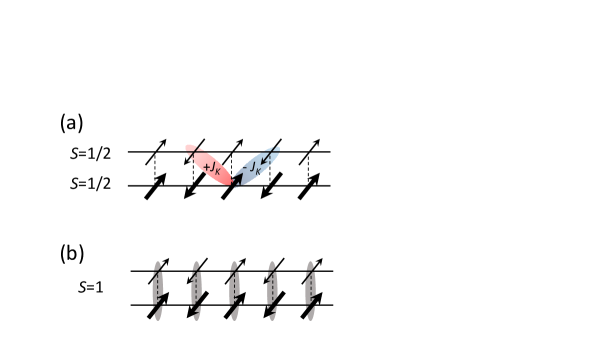
Figure 2: (a) At temperatures $T\ll\Delta_{c}\sim J_{K}^{2}$, the dynamically induced Mott gap, the charge degrees of freedom in the Hubbard chain become frozen and the system maps onto a ladder where the non-local antiferromagnetic Kondo coupling effectively induces local ferromagnetic correlations between the spins in the ladder (vertical dashed lines). (b) The system depicted in (a) can be mapped onto a $S=1$ Haldane chain, which supports topologically protected $S=1/2$ end-states Shelton et al. (1996); Gogolin et al. (1999b); Lecheminant and Orignac (2002); Affleck et al. (1987, 1989); Ng (1992, 1993, 1994).

The previous analysis shows that, at low temperatures $T\ll\Delta_{c}$, the 1D “$p-$wave” Kondo-Heisenberg chain at half-filling can be effectively mapped onto a spin ladder problem, which is dominated by the staggered components of the spin densities. Interestingly, for an antiferromagnetic Kondo coupling $J_{K}>0$, the negative sign emerging from the structure of the non-local Kondo interaction (24), effectively induces alocal ferromagnetic interaction [see vertical dashed lines in Fig. 2(a)]. It is well-known that the spin ladder with ferromagnetic exchange coupling $J_{\perp}<0$ along the rungs has a low-energy triplet sectorShelton et al. (1996); Gogolin et al. (1999b); Lecheminant and Orignac (2002), which maps onto the Haldane spin-1 chain Haldane (1983a, b). Therefore, at temperatures $T\ll J_{\perp}$, our model describes the physics of the Haldane spin-1 chain, which is known to host symmetry-protected topological spin-1/2 modes at the boundaries Affleck et al. (1987, 1989); Ng (1992, 1993, 1994); Berg et al. (2008); Gu and Wen (2009); Pollmann et al. (2010, 2012). This situation is also very reminiscent to the case of the ferromagnetic Kondo lattice Tsunetsugu et al. (1992); Garcia et al. (2004); Janani et al. (2014, 2014). To see how these spin-1/2 boundary modes emerge in our low-energy Hamiltonian (46), we consider solutions of the eigenvalue equation $\tilde{H}_{s}\Psi^{a}\left(x\right)=0$, where $\Psi^{a}\left(x\right)=\left(\xi_{R}^{a},\xi_{L}^{a}\right)^{T}$ is a Majorana spinor, and $a=\left(0,1,2,3\right)$ Lecheminant and Orignac (2002). In matrix form, this equation is

$$\left[-iv_{s}\hat{\tau}_{3}\partial_{x}+m_{a}\hat{\tau}_{2}\right]\Psi^{a}\left(x\right) =0,$$ (47)

with $m_{a}=-3J_{K}m_{2}m_{1}/2\pi$ for $a=0$ [$m_{a}=J_{K}m_{2}m_{1}/2\pi$ for $a=\left(1,2,3\right)$] and $\hat{\tau}_{i}$ the Pauli matrices acting of the right-, left-moving space. Eq. (47) admits solutions of the form $\Psi^{a}\left(x\right)\propto\exp\left(-m_{a}\hat{\tau}_{1}x/v_{s}\right)\Psi^{a}\left(0\right)$ and one would think that in principle two normalizable solutions in the limit $x\rightarrow\infty$ could arise: 1) the choice $\Psi^{a}\left(0\right)=\left(1,-1\right)^{T}$ with $m_{a}<0$, and 2) $\Psi^{a}\left(0\right)=\left(1,1\right)^{T}$ with $m_{a}>0$. However, note that only the last choice is compatible with the boundary condition (41). Then, the only physical solution localized around $x=0$ corresponds to the choice $m_{a}>0$, which in our case corresponds to $a=\left(1,2,3\right)$

$$\Psi^{a}\left(x\right)\propto\xi_{a}e^{-m_{a}x/v_{s}} \left(\begin{array}[]{c}1\\ 1\end{array}\right)\quad a=\left(1,2,3\right),$$ (50)

with $\xi_{a}$ being a localized Majorana fermion. Using the expression (43) for the smooth part of the spin density, we can physically associate the presence of the localized Majorana bound-state with a localized spin-1/2 magnetic edge-state. This is consistent with the results in Ref. Alexandrov and Coleman (2014) where, in the case of a uniform Kondo interaction, a magnetic mode with no admixture with charge degrees of freedom emerges at the boundaries. However, note that the origin of these edge-states is quite different: while in the mean-field regime they emerge as a consequence of Kondo-unscreened end-spins in the Heisenberg chain, in our case they are intimately related to the physics of the Haldane chain.

We now derive a topological invariant to characterize the presence of the edge-states, using a suitable generalization of the concept of electrical polarization in 1D insulators Resta and Sorella (1999); Ortiz and Martin (1994); Aligia and Batista (2005); Torio et al. (2006); Xiao et al. (2010); Fu and Kane (2006). We therefore focus on the uniform magnetization Eq. (43). Although the original Hamiltonian has spin-rotational symmetry, the Abelian bosonization is not an explicitly SU(2)-invariant formalism. Therefore, while the choice of axes is arbitrary due to the spin rotation symmetry of the problem, once we define the $z-$direction as the spin-quantization axis, the perpendicular components of the magnetization $M^{x}\left(x\right)$ and $M^{y}\left(x\right)$ acquire a more complicated mathematical form. For that reason, it is convenient to focus only on the $z$ component of the symmetric spin density Eq. (43)

$$M^{z}\left(x\right) =\sum_{\lambda=L,R}M_{1,\lambda}^{z}\left(x\right)+M_{2,\lambda}^{z}\left(x\right),$$

$$=-\frac{1}{\sqrt{\pi}}\partial_{x}\phi_{+}\left(x\right).$$ (51)

In the expression above, we have used Eq. (20) and the definition of $\phi_{+}\left(x\right)=\frac{1}{\sqrt{2}}\left[\phi_{1}\left(x\right)+\phi_{2}\left(x\right)\right]$. We now define the total magnetic moment along the $\hat{z}-$axis at one end (for concreteness, the left end) of the chain as $m_{T}^{z}\equiv\frac{1}{\sqrt{\pi}}\int_{0}^{x_{b}}dx\;M^{z}\left(x\right)$, where $x_{b}$ is an unspecified position in the interior of the chain where the magnetization reaches the value in the bulk. In bosonic language, it acquires the compact form

$$m_{T}^{z} =-\frac{1}{\pi}\left[\phi_{+}\left(x_{b}\right)-\phi_{+}\left(0\right)\right].$$ (52)

From the expression of the bosonic Hamiltonian Eq. (25) in the limit $J_{K}\rightarrow\infty$, we see that the system minimizes the energy in the bulk by pinning the field $\phi_{+}\left(x\right)$ to one of the degenerate values

$$\phi_{+}\left(x_{b}\right) =\pm\frac{\pi}{2}.$$ (53)

On the other hand, from the definition of $\phi_{\pm}\left(x\right)=\frac{1}{\sqrt{2}}\left[\phi_{1s}\left(x\right)\pm\phi_{2s}\left(x\right)\right]$ and Eq. (13), the boundary condition $\phi_{+}\left(0\right)=0$ is obtained. Replacing these values into Eq. (52), we obtain the following quantized values of the magnetic moment at the left end

$$m_{T}^{z} =\pm\frac{1}{2}.$$ (54)

This magnetic moment at the end of the chain is analogous to the electrical polarization Resta and Sorella (1999); Ortiz and Martin (1994); Aligia and Batista (2005); Torio et al. (2006); Xiao et al. (2010) or the time-reversal polarization Fu and Kane (2006) in 1D insulators. In particular, we note the close relation between our formula Eq. 52 and the expressions for the displacement operator appearing in Eq. (23) of Ref. Aligia and Batista (2005), and for the time-reversal polarization appearing in Eq. (4.8) in Ref. Fu and Kane (2006), both given in bosonic language. Frome here, we can define a $Z_{2}-$topological invariant which characterizes the topological phase of the Kondo-Heisenberg chain

$$Q =\left(-1\right)^{2m_{T}^{z}/\pi}=e^{i2\pi m_{T}^{z}},$$ (55)

which in the limit of an infinite system $L\rightarrow\infty$ is $Q=-1$ in the topological phase ($J_{K}>0$), and $Q=1$ in the trivial one ($J_{K}<0$).

The bosonic representation also provides an alternative way to demonstrate the existence of magnetic edge modes. Since none of the degenerate values (53) of $\phi_{+}\left(x\right)$ in the bulk satisfy the boundary condition at $x=0$, we conclude that a kink excitation necessarily must emerge near the boundary in order to connect those values: precisely this kink excitation gives rise to the spin-1/2 end-state, upon use of Eq. (51). We remind the reader that in Section III, using similar arguments, we demonstrated the absence of kink configurations in the charge field $\phi_{1c}\left(x\right)$, and the fact that there are no charge edge-states in the ground state.

V Conclusions

We have studied theoretically a model for a topological 1D Kondo insulator (the 1D Kondo-Heisenberg model coupled in the $p$-wave channel, with an on-site Hubbard interaction $U$ in the conduction band) using the Abelian bosonization formalism, and derived the two-loop RG flow equations for the system at half-filling. Our RG analysis shows that the system develops a Mott-insulating gap at low enough temperatures, even if $U=0$. Moreover, the remaining spin degrees of freedom are effectively described by a ferromagnetic spin-1/2 ladder, which in turn maps onto a spin-1 Haldane chain with topologically protected spin-1/2 magnetic edge-modes. This situation is reminiscent to the physics of the ferromagnetic Kondo necklace, which also maps onto the spin-1 Haldane chain Tsunetsugu et al. (1992); Garcia et al. (2004); Janani et al. (2014, 2014), although in our case it arises as a result of the non-trivial structure of the Kondo coupling.

In contrast to three-dimensional bulk topological Kondo insulators, where the mean-field approximation is well justified and the system can be effectively described in terms of non-interacting quasiparticles opening a (renormalized) hybridization gap near the Fermi surface Coleman (1984, 1987); Dzero et al. (2010), in one spatial dimension the presence of strong quantum fluctuations cannot be ignored, and one is forced to use different approaches. The Abelian bosonization method allows to obtain a description of the 1D TKI which is fundamentally different from the mean-field picture. In the first place, the system develops a Mott gap (instead of a hybridization gap) in the spectrum of charge excitations when the conduction band is half-filled (small deviations from half-filling do not affect this scenario qualitatively Giamarchi (2004)). This Mott gap arises from umklapp processes at second order in the Kondo interaction. Physically, this can be understood as a dynamically-induced effective interaction term, which appears at order $J_{K}^{2}$ in the conduction band by integrating out perturbatively short-time spin excitations in the Heisenberg chain. In contrast to the mean-field description, where the hybridization gap depends exponentially on the microscopic Kondo coupling $\Delta_{c}\sim\exp\left(-1/J_{K}\right)$, the integration of the RG Eqs. (34)-(36) in the limit $J_{K}\rightarrow 0$ results in $\Delta_{c}\sim J_{K}^{2}$ . Our RG analysis indicates that $J_{K}$ is a relevant perturbation and flows to strong coupling, dominating the physics at low temperatures. In particular, at temperatures below the Mott gap, the charge degrees of freedom are frozen and system effectively behaves as a ferromagnetic spin-1/2 ladder, which is known to map onto the spin-1 Haldane chain. Therefore, our work allows to make an insightful connection between two a priori unrelated physical models. Interestingly, exploiting this connection, we predict the existence of topologically protected spin-1/2 edge states. This seems to correspond to the “magnetic phase” found by Alexandrov and Coleman Alexandrov and Coleman (2014), which for a uniform Kondo coupling $J_{K}$, is characterized by Kondo-unscreened spins at the end of the Heisenberg chain. However, the emergence of these edge states, again corresponds to a very different mechanism than the one provided by the mean-field theory. Interestingly, within the bosonization framework, we have been able to obtain a $Z_{2}$ topological invariant [see Eq. (55)] in terms of the magnetization at an end of the chain.

Our work opens the possibility to explore the physics of broken $Z_{2}\times Z_{2}$ hidden symmetry and the existence of a non-vanishing string order parameter $\mathcal{O}_{\text{string}}^{\alpha}\equiv\lim_{\left|l-m\right|\rightarrow\infty}\left\langle S_{l}^{\alpha}e^{i\pi\sum_{l\leq j<m}S_{j}^{\alpha}}S_{m}^{\alpha}\right\rangle\neq 0$ (which are well-known features of the Haldane phase Kennedy and Tasaki (1992); Affleck et al. (1987, 1989)) in the $p-$wave Kondo-Heisenberg model. In particular, note the close relation between the $Z_{2}$ topological invariant (55) and the string-order parameter in bosonized form [see Eq. (83) in Ref. Shelton et al. (1996)].

Furthermore, we reiterate that the model studied here can be viewed as a non-trivial strongly-correlated generalization of the old Tamm-Shockley model Tamm (1932); Shockley (1939). The latter is a prototypical one-dimensional model that exhibits a topological phase transition and it can be used to construct high-dimensional topological band insulators Pershoguba and Yakovenko (2012). Likewise, the strongly-correlated topological Kondo-Heisenberg model could potentially become a building block in constructing higher-dimensional strongly-interacting topological states – not adiabatically connected to “simple” topological band insulators. Although the physical realization of the 1D $p$-wave Kondo lattice model studied here in solid-state systems might be quite challenging, our results might have direct application to ultracold atom experiments, where double-well optical superlattices loaded with atoms in $s$ and $p$ orbitals have been realized Wirth et al. (2011); Soltan-Panahi et al. (2012). In such systems, one can imagine the atoms forming ladders where one of the legs corresponds to the $s$ orbitals and the other to $p$ orbitals (e.g., see Ref. Li et al. (2013)). The overlap between $s$ and $p$ orbitals along the rungs vanish by symmetry, and therefore only the off-diagonal hopping $t_{sp}$ survives. Next, allowing for an on-site repulsive Hubbard $U^{\prime}$ interaction in the $s$-orbital leg (using, e.g., Feschbach resonances), one can derive an effective $p$-wave Kondo lattice model in the limit $t_{sp}/U\rightarrow 0$, introducing a canonical transformation to eliminate processes at first order in $t_{sp}$. At half-filling, the $s$-orbitals are effectively described by SU(2) spins and the Kondo parameter in our Eq. (3) becomes proportional to $J_{K}\sim t_{sp}^{2}/U$. Therefore, the system can be described by the model described in this work. Finally, we mention in this context recent experimental results Nakajima et al. (2013); Eo et al. (2014); Fuhrman et al. (2014), which suggest the existence of a magnetic phase transition and/or suppressed surface charge transport in select samples of Samarium hexaboride ($\text{SmB}_{6}$ – a three-dimensional topological Kondo insulator). It is possible that these phenomena, which remain unexplained at this stage, involve in a crucial way an interplay between band topology and strong correlations, which conceivably may lead to the formation of non-trivial magnetic topological surface modes reminiscent to the edge states found here. In a more general context, our results might be relevant to other materials which belong to the same “Haldane universality class”, thanks to the connection (unveiled in this work) to the ferromagnetic Kondo lattice model. For example, the organic molecular compound Mo₃S₇(dmit)₃ at two-third filling, a promising candidate for a quantum spin liquid, has recently been shown to be a realization of the ferromagnetic Kondo lattice model at half-filling Janani et al. (2014, 2014), and therefore it should realize a Haldane phase with magnetic end-modes at low temperatures.

A. M. L. acknowledges support from National Science Foundation-Joint Quantum Institute- Physics Frontier Center (NSF-JQ-PFC) and from program Red de Argentinos Investigadores y Científicos en el Exterior (RAICES), Argentina. A. O. D. is partially supported by Proyecto de Investigación Plurianual (PIP) 11220090100392 of Consejo de Investigaciones Científicas y Técnicas (CONICET), Argentina. V. G. was supported by Department of Energy- Basic Energy Sciences (DOE-BES) DESC0001911 and Simons Foundation. The authors would like to thank Thierry Giamarchi, Eduardo Fradkin, Philippe Lecheminant, Edmond Orignac, Dmitry Efimkin, Xiaopeng Li and Tigran Sedrakyan for useful discussions and for pointing out relevant references.

Appendix A Dynamically-generated interactions and derivation of the renormalization group equations

In this Appendix we derive an effective action for the system and the renormalization-group (RG) equations (34-36). The idea is to show that umklapp processes, which mimic a repulsive interaction among electrons in the half-filled conduction band, arise at order $\mathcal{O}\left(J_{K}^{2}\right)$ and open a gap in the charge sector of the model. To that end, we expand the generating functional of the system (i.e., the partition function) up to second order in the coupling constants $G_{\alpha}$ following Refs. Cardy (1996); Fradkin (2013)

$$\frac{Z}{Z_{0}} =\left[1-\sum_{\alpha}\frac{G_{\alpha}}{a^{2-\Delta_{\alpha}}}\int d^{2}r\left\langle O_{\alpha}\right\rangle_{0}+\frac{1}{2}\sum_{\alpha,\beta}\frac{G_{\alpha}G_{\beta}}{a^{4-\Delta_{\alpha}-\Delta_{\beta}}}\int\int_{\left|r-r^{\prime}\right|>a}d^{2}rd^{2}r^{\prime}\left\langle O_{\alpha}\left(r\right)O_{\beta}\left(r^{\prime}\right)\right\rangle_{0}+...\right]$$ (A.1)

indexes $\alpha$ and $\beta$ run on $2c$, $3$ and $K$. Here, $\Delta_{\alpha}$ is the scaling dimension of the operator $O_{\alpha}$ defined in Eqs. (31-33) ($\Delta_{3}=\Delta_{2c}=2$, $\Delta_{K}=\frac{3}{2}$), $Z_{0}=\int\prod_{i=\left\{1c,\pm\right\}}\mathcal{D}\left[\phi_{i},\theta_{i}\right]\;e^{-S_{0}\left[\phi_{i},\theta_{i}\right]}$ is the generating function of the free theory, and the mean values $\left\langle\dots\right\rangle_{0}$ correspond also to that theory. This formalism is standard in the analysis of 1D quantum systems, and has been applied in several previous works (see for example Ref. Dobry and Aligia (2011) where the method is explained in detail).

The third term of the r.h.s. in Eq. (A.1) takes the same form as the second one if we assume that for $r\rightarrow r^{\prime}$ the product of two operators fulfills the following operator product expansion (OPE) property Cardy (1996); Fradkin (2013) :

$$O_{\alpha}\left(r\right)O_{\beta}\left(r^{\prime}\right) =\sum_{\gamma}C_{\alpha\beta}^{\gamma}\frac{O_{\gamma}\left(\frac{r+r^{\prime}}{2}\right)}{\mid r-r^{\prime}\mid^{\Delta_{\alpha}+\Delta_{\beta}-\Delta_{\gamma}}}+\mbox{more irrelevant operators.}$$ (A.2)

where $O_{\gamma}$ includes all the operators generated from each OPE.

Let us focus on the OPE between two $O_{K}$ operators, which is the most relevant perturbation in the RG sense, and is precisely the contribution that leads to the umklapp processes we are trying to describe. To simplify the discussion, here we return to the representation of the bosonic fields in terms of left and right movers $\phi_{L}\left(z\right)$ and $\phi_{R}\left(\bar{z}\right)$ [see Eq. (8)], with $z=v_{F}\tau+ix$ and $\bar{z}=v_{F}\tau-ix$. We now assume to be sufficiently deep in the bulk of the 1D system and far away from the boundaries. In these conditions, the boundary conditions (9) and (10), and the commutation relation (11) can be effectively neglected, and the fields $\phi_{L}\left(z\right)$ and $\phi_{R}\left(\bar{z}\right)$ become independent (i.e., they do not mix). This allows us to focus only on the processes involving the left-moving field $\phi_{L}\left(z\right)$(for right-moving fields we just need to change $L\rightarrow R$ and $z\rightarrow\bar{z}$) . The basic OPE we need is

$$\colon e^{i\lambda\phi_{L}\left(z\right)}\colon\colon e^{i\lambda^{\prime}\phi_{L}\left(z^{\prime}\right)}\colon =\left(\frac{2\pi}{L}\right)^{\frac{\lambda\lambda^{\prime}}{2}}\colon e^{i\left(\lambda+\lambda^{\prime}\right)\phi_{L}\left(z^{\prime}\right)}\left[\frac{1}{\left(z-z^{\prime}\right)^{-\lambda\lambda^{\prime}}}+\frac{i\lambda\partial_{z^{\prime}}\phi_{L}\left(z^{\prime}\right)}{\left(z-z^{\prime}\right)^{-\lambda\lambda^{\prime}-1}}+...\right]\colon$$ (A.3)

which was obtained by normal-ordering the rhs expression and then developing for $z^{\prime}$ near $z$. Through repeated use of this expression we obtain the desired OPE which reads:

$$O_{K}\left(z,\overline{z}\right)O_{K}\left(z^{\prime},\overline{z}^{\prime}\right)= -\frac{3}{4\pi}\frac{O_{3}}{\mid z-z^{\prime}\mid}-\frac{3}{4\pi}\frac{O_{2c}}{\mid z-z^{\prime}\mid}$$

$$+\frac{3}{4\pi}\frac{O_{-}}{\mid z-z^{\prime}\mid}-\frac{1}{4\pi}\frac{O_{+}}{\mid z-z^{\prime}\mid},$$ (A.4)

where we have defined the operators $O_{\pm}\equiv\frac{1}{4\pi}\partial_{\overline{z}}\phi_{\pm R}\partial_{z}\phi_{\pm L}$ [which also appear in the $z$-component of the product of the right and left smooth-varying spin currents, in the first two lines in Eq. (3.8) of Ref. Dobry et al. (2013)]. Note that these terms break the SU(2) invariance of the model. This is a well-known feature of the Abelian bosonization prescription, which is not explicitly SU(2)-invariant formalism Giamarchi (2004); Gogolin et al. (1999a). This means that one has to keep track of all contributions to recover the SU(2) invariance and, vice versa, neglecting irrelevant operators [as we did to obtain the action in Eq.(26)] might result in apparent inconsistencies in the formalism. In our case, this problem has no consequences for our purposes because the operators $O_{\pm}$ renormalize the couplings of the marginal contributions, which we in any case we have neglected in relation to the relevant contribution $\sim:\mathbf{N}_{1}\cdot\mathbf{N}_{2}:$. Therefore, we will not consider these operators.

On the other hand, the first line in Eq. (A.4) is physically more interesting, as the operators $O_{3}$ and $O_{2c}$ were already present in the action (28) corresponding to the Hubbard model. If we insert (A.4) into (A.1), change variables as $\hat{r}=r-r^{\prime}$ and $R=\frac{r+r^{\prime}}{2}$ and integrate over $\hat{r}$ imposing a cutoff of order $a$, we obtain an expression that renormalizes the first order contribution. We identify the effective coupling for operators $O_{2c}$ and $O_{3}$ as:

$$\hat{G}_{2c}^{0} =G_{2c}^{0}+\frac{3}{8}G_{K}^{2}$$ (A.5)

and the same for $\hat{G}_{3}^{0}$. Therefore, we have shown that the interchain Kondo coupling generates an effective Hubbard repulsion $U_{eff}=\frac{3a}{8}\frac{(J_{K}m_{2})^{2}}{\pi v_{F}}$ in the conduction chain. The equation above can be physically interpreted as umklapp processes (generated by integrating out fast spin fluctuations in the Heisenberg chain at second order in the interchain Kondo coupling) which mimic the effect of an interaction in the conduction band.

To determine the actual dependence of the charge gap $\Delta_{c}$ with respect to the parameters of the model, we need to derive the RG flow equations. This is achieved following similar step as in the previous paragraphs. The main idea is that the theory defined with a microscopic cutoff $a$ should remain invariant under a scaling transformation $a\rightarrow a\left(1+dl\right)$, where $dl$ is a dimensionless infinitesimal. Therefore, the couplings $G_{\alpha}\left(a\right)$ in Eq. (A.1) must be changed in such a way that they preserve the generating functional, i.e., $Z\left[a\right]=Z\left[a\left(1+dl\right)\right]$. The method is standard and we refer the reader to Ref. Cardy (1996) for details. The renormalization group flow equations can be written in terms of the coefficients $C_{\alpha\beta}^{\gamma}$ as

$$\frac{dG_{\gamma}}{dl} =\left(2-\Delta_{\gamma}\right)G_{\gamma}-\pi\sum_{\alpha\beta}C_{\alpha\beta}^{\gamma}G_{\alpha}G_{\beta},$$ (A.6)

where the coefficients $C_{KK}^{2c}=C_{KK}^{3}=-\frac{3}{4\pi}$ are extracted from Eq. (A.4). The remaining coefficients are obtained by the OPEs between the corresponding operators. Following the lines of Ref. von Delft and Schoeller (1998) we obtain straightforwardly:

$$C_{2c\;3}^{3}=-\frac{1}{2\pi},\qquad C_{3\;3}^{2c}=-\frac{1}{\pi}$$

$$C_{2c\;K}^{K}=-\frac{1}{8\pi},\qquad C_{3\;K}^{K}=-\frac{1}{2\pi}$$ (A.7)

Inserting these values in Eq. (A.6) we obtain Eqs. (34)-(36) in the main text.

References

- Kane and Mele (2005a) C. L. Kane and E. J. Mele, Topological Order and the Quantum Spin Hall Effect, Phys. Rev. Lett. 95, 146802 (2005a).
- Kane and Mele (2005b) C. L. Kane and E. J. Mele, Quantum Spin Hall Effect in Graphene, Phys. Rev. Lett. 95, 226801 (2005b).
- Moore and Balents (2007) J. E. Moore and L. Balents, Topological invariants of time-reversal-invariant band structures, Phys. Rev. B 75, 121306 (2007).
- Roy (2009) R. Roy, classification of quantum spin Hall systems: An approach using time-reversal invariance, Phys. Rev. B 79, 195321 (2009).
- Fu et al. (2007) L. Fu, C. L. Kane, and E. J. Mele, Topological Insulators in Three Dimensions, Phys. Rev. Lett. 98, 106803 (2007).
- Hasan and Kane (2010) M. Z. Hasan and C. L. Kane, Colloquium : Topological insulators, Rev. Mod. Phys. 82, 3045 (2010).
- Qi and Zhang (2011) X.-L. Qi and S.-C. Zhang, Topological insulators and superconductors, Rev. Mod. Phys. 83, 1057 (2011).
- Bernevig and Hughes (2013) B. A. Bernevig and T. L. Hughes, Topological Insulators and Topological Superconductors (Princeton University Press, 2013).
- Kitaev (2009) A. Kitaev, Periodic table for topological insulators and superconductors, AIP Conf. Proc. 1134, 22 (2009).
- Ryu et al. (2010) S. Ryu, A. P. Schnyder, A. Furusaki, and A. W. W. Ludwig, Topological insulators and superconductors: tenfold way and dimensional hierarchy, New Journal of Physics 12, 065010 (2010).
- Hsieh et al. (2008) D. Hsieh, D. Qian, L. Wray, Y. Xia, Y. S. Hor, R. J. Cava, and M. Z. Hasan, A topological Dirac insulator in a quantum spin Hall phase, Nature 452, 970 (2008).
- Xia et al. (2009) Y. Xia, D. Qian, L. Hsieh, D. Wray, A. Pal, H. Lin, A. Bansil, D. Grauer, Y. S. Hor, R. J. Cava, and M. Z. Hasan, Observation of a large-gap topological-insulator class with a single Dirac cone on the surface, Nat. Phys. 5, 398 (2009).
- König et al. (2007) M. König, S. Wiedmann, C. Brüne, A. Roth, H. Buhmann, L. W. Molenkamp, X.-L. Qi, and S.-C. Zhang, Quantum Spin Hall Insulator State in HgTe Quantum Wells, Science 318, 766 (2007).
- Knez et al. (2011) I. Knez, R.-R. Du, and G. Sullivan, Evidence for Helical Edge Modes in Inverted InAs/GaSb Quantum Wells, Phys. Rev. Lett. 107, 136603 (2011).
- Nowack et al. (2013) K. C. Nowack, E. M. Spanton, M. Baenninger, M. König, J. R. Kirtley, B. Kalisky, C. Ames, P. Leubner, C. Brüne, H. Buhmann, L. W. Molenkamp, D. Goldhaber-Gordon, and K. A. Moler, Imaging currents in HgTe quantum wells in the quantum spin Hall regime, Nat. Mater. 12, 787 (2013).
- Spanton et al. (2014) E. M. Spanton, K. C. Nowack, L. Du, G. Sullivan, R.-R. Du, and K. A. Moler, Images of Edge Current in InAs/GaSb Quantum Wells, Phys. Rev. Lett. 113, 026804 (2014).
- Dzero et al. (2010) M. Dzero, K. Sun, V. Galitski, and P. Coleman, Topological Kondo Insulators, Phys. Rev. Lett. 104, 106408 (2010).
- Read and Newns (1983) N. Read and D. M. Newns, On the solution of the Coqblin-Schreiffer Hamiltonian by the large-N expansion technique, J. Phys. C 16, 3273 (1983).
- Coleman (1987) P. Coleman, Mixed valence as an almost broken symmetry, Phys. Rev. B 35, 5072 (1987).
- Newns and Read (1987) D. M. Newns and N. Read, Mean-field theory of intermediate valence/heavy fermion systems, Adv.Phys. 36, 799 (1987).
- Reich (2012) E. S. Reich, Hopes surface for exotic insulator, Nature 492, 165 (2012).
- Zhang et al. (2013) X. Zhang, N. P. Butch, P. Syers, S. Ziemak, R. L. Greene, and J. Paglione, Hybridization, Inter-Ion Correlation, and Surface States in the Kondo Insulator , Phys. Rev. X 3, 011011 (2013).
- Kim et al. (2013) D. Kim, S. Thomas, T. Grant, J. Botimer, Z. Fisk, and J. Xia, Surface Hall Effect and Nonlocal Transport in SmB6: Evidence for Surface Conduction, Scientific Reports 3, 3150 (2013).
- Wolgast et al. (2013) S. Wolgast, C. Kurdak, K. Sun, J. W. Allen, D.-J. Kim, and Z. Fisk, Low-temperature surface conduction in the Kondo insulator SmB6, Phys. Rev. B 88, 180405 (2013).
- Neupane et al. (2013) M. Neupane, N. Alidoust, S. Xu, T. Kondo, Y. Ishida, D.-J. Kim, C. Liu, I. Belopolski, Y. Jo, T.-R. Chang, H.-T. Jeng, T. Durakiewicz, L. Balicas, H. Lin, A. Bansil, S. Shin, Z. Fisk, and M. Z. Hasan, Surface electronic structure of the topological Kondo-insulator candidate correlated electron system SmB6, Nature Commun. 4, 2991 (2013).
- Alexandrov and Coleman (2014) V. Alexandrov and P. Coleman, End states in a one-dimensional topological Kondo insulator in large- limit, Phys. Rev. B 90, 115147 (2014).
- Wirth et al. (2011) G. Wirth, M. Ölschläger, and A. Hemmerich, Evidence for orbital superfluidity in the p-band of bipartite optical square lattice, Nat. Phys. 7, 147 (2011).
- Soltan-Panahi et al. (2012) P. Soltan-Panahi, D.-S. Lühmann, J. Struck, P. Windpassinger, and K. Sengstock, Quantum phase transition to unconventional multi-orbital superfluidity in optical lattices, Nat. Phys. 8, 71 (2012).
- Nakajima et al. (2013) Y. Nakajima, P. S.Syers, X. Wang, R. Wang, and J. Paglione, One-dimensional edge state transport in a topological Kondo insulator, arXiv:1312.6132 (2013).
- Eo et al. (2014) Y. S. Eo, S. Wolgast, T. Ozturk, G. Li, Z. Xiang, C. Tinsman, T. Asaba, F. Yu, B. Lawson, J. W. Allen, K. Sun, L. Li, C. Kurdak, D.-J. Kim, and Z. Fisk, Hysteretic Magnetotransport in SmB6 at Low Magnetic Fields (2014), arXiv:1410.7430 [cond-mat.str-el] .
- Fuhrman et al. (2014) W. T. Fuhrman, J. Leiner, P. Nikolić, G. E. Granroth, M. B. Stone, M. D. Lumsden, L. DeBeer-Schmitt, P. A. Alekseev, J.-M. Mignot, S. M. Koohpayeh, P. Cottingham, W. A. Phelan, L. Schoop, T. M. McQueen, and C. Broholm, Spin-exciton and topology in SmB$_6$ (2014), arXiv:1407.2647 [cond-mat.str-el] .
- Tamm (1932) I. Tamm, On the possible bound states of electrons on a crystal surface, Physik. Zeits. Soviet Union 1, 733 (1932).
- Shockley (1939) W. Shockley, On the Surface States Associated with a Periodic Potential, Phys. Rev. 56, 317 (1939).
- Pershoguba and Yakovenko (2012) S. S. Pershoguba and V. M. Yakovenko, Shockley model description of surface states in topological insulators, Phys. Rev. B 86, 075304 (2012).
- Li et al. (2013) X. Li, E. Zhao, and V. Liu, Topological states in a ladder-like optical lattice containing ultracold atoms in higher orbital bands, Nature Communications 4, 1523 (2013).
- Giamarchi (2004) T. Giamarchi, Quantum Physics in One Dimension (Oxford University Press, Oxford, 2004).
- Gogolin et al. (1999a) A. O. Gogolin, A. A. Nersesyan, and A. M. Tsvelik, Bosonization and Strongly Correlated Systems (Cambridge University Press, Cambridge, 1999).
- Lecheminant and Orignac (2002) P. Lecheminant and E. Orignac, Magnetization and dimerization profiles of the cut two-leg spin ladder and spin-1 chain, Phys. Rev. B 65, 174406 (2002), cond-mat/0111177 .
- von Delft and Schoeller (1998) J. von Delft and H. Schoeller, Bosonization for beginners - refermionization for experts, Ann. Phys. (Leipzig) 7, 225 (1998).
- Zachar et al. (1996) O. Zachar, S. A. Kivelson, and V. J. Emery, Exact Results for a 1D Kondo Lattice from Bosonization, Phys. Rev. Lett. 77, 1342 (1996).
- Sikkema et al. (1997) A. E. Sikkema, I. Affleck, and S. R. White, Spin Gap in a Doped Kondo Chain, Phys. Rev. Lett. 79, 929 (1997).
- Zachar and Tsvelik (2001) O. Zachar and A. M. Tsvelik, One dimensional electron gas interacting with a Heisenberg spin-1/2 chain, Phys. Rev. B 64, 033103 (2001), cond-mat/9909296.
- Zachar (2001) O. Zachar, Staggered liquid phases of the one-dimensional Kondo-Heisenberg lattice model, Phys. Rev. B 63, 205104 (2001).
- Berg et al. (2010) E. Berg, E. Fradkin, and S. A. Kivelson, Pair-Density-Wave Correlations in the Kondo-Heisenberg Model, Phys. Rev. Lett. 105, 146403 (2010).
- Dobry et al. (2013) A. Dobry, A. Jaefari, and E. Fradkin, Inhomogeneous superconducting phases in the frustrated Kondo-Heisenberg chain, Phys. Rev. B 87, 245102 (2013).
- Cho et al. (2014) G. Y. Cho, R. Soto-Garrido, and E. Fradkin, Topological Pair-Density-Wave Superconducting States, ArXiv e-prints (2014), arXiv:1407.6358 [cond-mat.str-el] .
- Shelton et al. (1996) D. G. Shelton, A. A. Nersesyan, and A. M. Tsvelik, Antiferromagnetic spin ladders: Crossover between spin S =1/2 and S =1 chains, Phys. Rev. B 53, 8521 (1996).
- Gogolin et al. (1999b) A. O. Gogolin, A. A. Nersesyan, A. M. Tsvelik, and L. Yu, Zero-modes and thermodynamics of disordered spin-1/2 ladders, Nucl. Phys. B 540, 705 (1999b).
- Robinson et al. (2012) N. J. Robinson, F. H. L. Essler, E. Jeckelmann, and A. M. Tsvelik, Finite wave vector pairing in doped two-leg ladders, Phys. Rev. B 85, 195103 (2012).
- Affleck et al. (1987) I. Affleck, T. Kennedy, E. H. Lieb, and H. Tasaki, Rigorous results on valence-bond ground states in antiferromagnets, Phys. Rev. Lett. 59, 799 (1987).
- Affleck et al. (1989) I. Affleck, T. Kennedy, E. H. Lieb, and H. Tasaki, Valence bond ground states in isotropic quantum antiferromagnets, Commun. Math. Phys. 115, 477 (1989).
- Ng (1992) T. K. Ng, Schwinger boson mean-field theory for open spin chain, Phys. Rev. B 45, 8181 (1992).
- Ng (1993) T. K. Ng, Edge states in Schwinger-boson mean-field theory of low-dimensional quantum antiferromagnets, Phys. Rev. B 47, 11575 (1993).
- Ng (1994) T. K. Ng, Edge states in antiferromagnetic quantum spin chains, Phys. Rev. B 50, 555 (1994).
- Haldane (1983a) F. D. M. Haldane, Continuum dynamics of the 1-D Heisenberg antiferromagnet: Identification with the O(3) nonlinear sigma model, Phys. Lett. A 93, 464 (1983a).
- Haldane (1983b) F. D. M. Haldane, Nonlinear Field Theory of Large-Spin Heisenberg Antiferromagnets: Semiclassically Quantized Solitons of the One-Dimensional Easy-Axis Néel State, Phys. Rev. Lett. 50, 1153 (1983b).
- Berg et al. (2008) E. Berg, E. G. Dalla Torre, T. Giamarchi, and E. Altman, Rise and fall of hidden string order of lattice bosons, Phys. Rev. B 77, 245119 (2008).
- Gu and Wen (2009) Z.-C. Gu and X.-G. Wen, Tensor-entanglement-filtering renormalization approach and symmetry-protected topological order, Phys. Rev. B 80, 155131 (2009).
- Pollmann et al. (2010) F. Pollmann, A. M. Turner, E. Berg, and M. Oshikawa, Entanglement spectrum of a topological phase in one dimension, Phys. Rev. B 81, 064439 (2010).
- Pollmann et al. (2012) F. Pollmann, E. Berg, A. M. Turner, and M. Oshikawa, Symmetry protection of topological phases in one-dimensional quantum spin systems, Phys. Rev. B 85, 075125 (2012).
- Tsunetsugu et al. (1992) H. Tsunetsugu, Y. Hatsugai, K. Ueda, and M. Sigrist, Spin-liquid ground state of the half-filled Kondo lattice in one dimension, Phys. Rev. B 46, 3175 (1992).
- Garcia et al. (2004) D. J. Garcia, K. Hallberg, B. Alascio, and M. Avignon, Spin Order in One-Dimensional Kondo and Hund Lattices, Phys. Rev. Lett. 93, 177204 (2004).
- Janani et al. (2014) C. Janani, J. Merino, I. P. McCulloch, and B. J. Powell, Low-energy effective theories of the two-thirds filled Hubbard model on the triangular necklace lattice, Phys. Rev. B 90, 035120 (2014).
- Janani et al. (2014) C. Janani, J. Merino, I. P. McCulloch, and B. J. Powell, Topological spin liquid phase in a low-dimensional organic molecular compound, ArXiv e-prints (2014), arXiv:1401.6605 [cond-mat.str-el] .
- Resta and Sorella (1999) R. Resta and S. Sorella, Electron Localization in the Insulating State, Phys. Rev. Lett. 82, 370 (1999).
- Ortiz and Martin (1994) G. Ortiz and R. M. Martin, Phys. Rev. B 49, 14202 (1994).
- Aligia and Batista (2005) A. A. Aligia and C. D. Batista, Dimerized phase of ionic Hubbard models, Phys. Rev. B 71, 125110 (2005).
- Torio et al. (2006) M. E. Torio, A. A. Aligia, G. I. Japaridze, and B. Normand, Quantum phase diagram of the generalized ionic Hubbard model for chains, Phys. Rev. B 73, 115109 (2006).
- Xiao et al. (2010) D. Xiao, M.-C. Chang, and Q. Niu, Berry phase effects on electronic properties, Rev. Mod. Phys. 82, 1959 (2010).
- Fu and Kane (2006) L. Fu and C. L. Kane, Time reversal polarization and a adiabatic spin pump, Phys. Rev. B 74, 195312 (2006).
- Coleman (1984) P. Coleman, New approach to the mixed-valence problem, Phys. Rev. B 29, 3035 (1984), the idea of slave bosons seems to go back to S.E. Barnes, J. Phys. F 6, 1374 (1976).
- Kennedy and Tasaki (1992) T. Kennedy and H. Tasaki, Hidden symmetry breaking in Haldane gap antiferromagnets, Phys. Rev. B 45, 304 (1992).
- Cardy (1996) J. Cardy, Scaling and Renormalization in Statistical Physics (Cambridge University Press, Cambridge, 1996).
- Fradkin (2013) E. Fradkin, Field theories of condensed matter systems (2nd Edition) (Cambridge University Press, New York, 2013).
- Dobry and Aligia (2011) A. O. Dobry and A. A. Aligia, Quantum phase diagram of the half filled Hubbard model with bond-charge interaction, Nuclear Physics B 843, 767 (2011), arXiv:1009.4113 .