End-to-End Integration of a
Convolutional Network, Deformable Parts Model
and Non-Maximum Suppression

Abstract

Deformable Parts Models and Convolutional Networks each have achieved notable performance in object detection. Yet these two approaches find their strengths in complementary areas: DPMs are well-versed in object composition, modeling fine-grained spatial relationships between parts; likewise, ConvNets are adept at producing powerful image features, having been discriminatively trained directly on the pixels. In this paper, we propose a new model that combines these two approaches, obtaining the advantages of each. We train this model using a new structured loss function that considers all bounding boxes within an image, rather than isolated object instances. This enables the non-maximal suppression (NMS) operation, previously treated as a separate post-processing stage, to be integrated into the model. This allows for discriminative training of our combined Convnet + DPM + NMS model in end-to-end fashion. We evaluate our system on PASCAL VOC 2007 and 2011 datasets, achieving competitive results on both benchmarks.

1 Introduction

Object detection has been addressed using a variety of approaches, including sliding-window Deformable Parts Models [5, 19, 6], region proposal with classification [7, 16], and location regression with deep learning [13, 14]. Each of these methods have their own advantages, yet are by no means mutually exclusive. In particular, structured parts models capture the composition of individual objects from component parts, yet often use rudimentary features like HoG [2] that throw away much of the discriminative information in the image. By contrast, deep learning approaches [9, 18, 13], based on Convolutional Networks [10], extract strong image features, but do not explicitly model object composition. Instead, they rely on pooling and large fully connected layers to combine information from spatially disparate regions; these operations can throw away useful fine-grained spatial relationships important for detection.

Figure 1: An overview of our system: (i) a convolutional network extracts features from an image pyramid; (ii) a set of deformable parts models (each capturing a different view) are applied to the convolutional feature maps; (iii) non-maximal suppression is applied to the resulting response maps, yielding bounding box predictions. Training is performed using a new loss function that enables back-propagation through all stages.

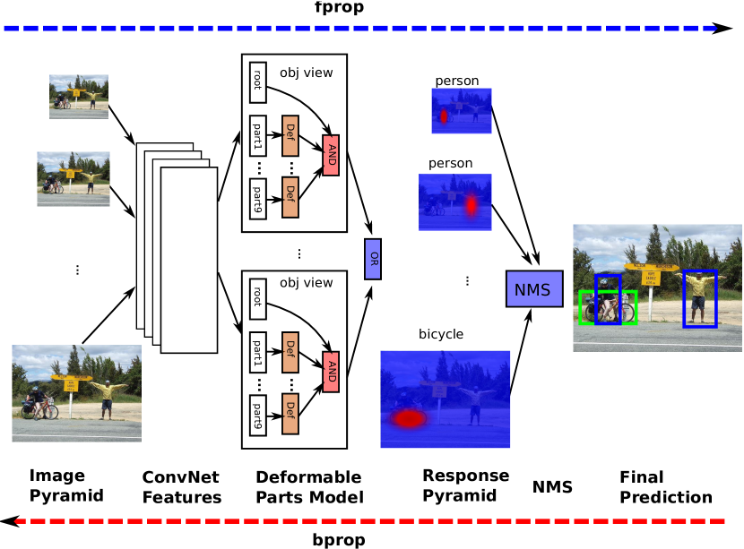
In this paper, we propose a framework (shown in Fig. 1) that combines these two approaches, fusing together structured learning and deep learning to obtain the advantages of each. We use a DPM for detection, but replace the HoG features with features learned by a convolutional network. This allows the use of complex image features, but still preserves the spatial relationships between object parts during inference.

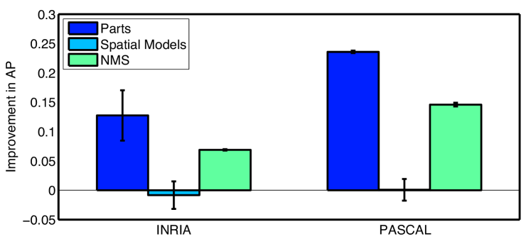
An often overlooked aspect of many detection systems is the non-maximal suppression stage, used to winnow multiple high scoring bounding boxes around an object instance down to a single detection. Typically, this is a post-processing operation applied to the set of bounding boxes produced by the object detector. As such, it is not part of the loss function used to train the model and any parameters must be tuned by hand. However, as demonstrated by Parikh and Zitnick [11], NMS can be a major performance bottleneck (see Fig. 2). We introduce a new type of image-level loss function for training that takes into consideration of all bounding boxes within an image. This differs with the losses used in existing frameworks that consider single cropped object instances. Our new loss function enables the NMS operation trained as part of the model, jointly with the Convnet and DPM components.

Figure 2: Reproduced from Parikh and Zitnick [11]: an ablation study of the stages in a DPM model [5] . Their figure shows how significant performance improvements could be obtained by replacing the parts detection and non-maximal suppresssion stages with human subjects. This suggests that these stages limit performance within the model. Our work focuses on improving each of these, replacing the part detectors with a Convnet and integrating NMS into the model.

2 Related Work

Most closely related is the concurrent work of Girshick et al.  [8], who also combine a DPM with ConvNet features in a model called DeepPyramid DPM (DP-DPM). Their work, however, is limited to integrating fixed pretrained ConvNet features with a DPM. We independently corroborate the conclusion that using ConvNet features in place of HoG greatly boosts the performance of DPMs. Furthermore, we show how using a post-NMS online training loss improves response ordering and addresses errors from the NMS stage. We also perform joint end-to-end training of the entire system.

The basic building blocks of our model architecture come from the DPMs of Felzenszwalb et al. [5] and Zhu et al.  [19][1], and the ConvNet of Krizhevsky et al. [9]. We make crucial modifications in their integration that enables the resulting model to achieve competitive object detection performance. In particular, we develop ways to transfer the ConvNet from classification to the detection environment, as well as changes to the learning procedure to enable joint training of all parts.

The first system to combine structured learning with a ConvNet is LeCun et al. [10], who train a ConvNet to classify individual digits, then train with hand written strings of digits discriminatively. Very recently, Tompson et al. [15] trained a model for human pose estimation that combines body part location estimates into a convolutional network, in effect integrating an MRF-like model with a ConvNet. Their system, however, requires annotated body part locations and is applied to pose estimation, whereas our system does not require annotated parts and is applied to object detection.

Some recent works have applied ConvNets to object detection directly: Sermanet et al. [13] train a network to regress on object bounding box coordinates at different strides and scales, then merge predicted boxes across the image. Szegedy et al. [14] regress to a bitmap with the bounding box target, which they then apply to strided windows. Both of these approaches directly regress to the bounding box from the convolutional network features, potentially ignoring many important spatial relationships. By contrast, we use the ConvNet features as input to a DPM. In this way, we can include a model of the spatial relationships between object parts.

In the R-CNN model, Girshick et al. [7] take a different approach in the use of ConvNets. Instead of integrating a location regressor into the network, they instead produce candidate region proposals with a separate mechanism, then use the ConvNet to classify each region. However, this explicitly resizes each region to the classifier field of view (fixed size), performing significant distortions to the input, and requires the entire network stack to be recomputed for each region. Instead, our integration runs the features in a convolutional bottom-up fashion over the whole image, preserving the true aspect ratios and requiring only one computational pass.

End-to-end training of a multi-class detector and post-processing has also been discussed in Desai et al.  [3]. Their approach reformulates NMS as a contextual relationship between locations. They replace NMS, which removes duplicate detections, with a greedy search that adds detection results using an object class-pairs context model. Whereas their system handles interactions between different types of objects, our system integrates NMS in a way that creates an ordering of results both of different classes and the same class but different views. In addition, we further integrate this into a full end-to-end system including ConvNet feature generation.

3 Model Architecture

Figure 3: Our model architecture, with Convolutional Network (left), Deformable Parts Model (right) and non-maximal suppression (top) components. An input $x$ is first repeatedly downsampled to create an image pyramid (a). We run the convolutional network on each scale, by performing four layers of convolution and max-pooling operations (b.ii - b.iv). This produces a set of appearance features $\phi_{A}(x_{s})$ at each scale, which are used as input to a DPM (c.i). Each object class model has three views of object templates (c.ii), each of which is composed of a root filter and nine parts filters. These produce a response map $F_{v}$ for each view (c.iii), which are then combined using a pixel-wise max (c.iv) to form a final activation map for the object class, $F(x_{s},y)$. We then perform NMS (d) across responses for all scales. To generate bounding boxes, we trace the activation locations back to their corresponding boxes in the input.

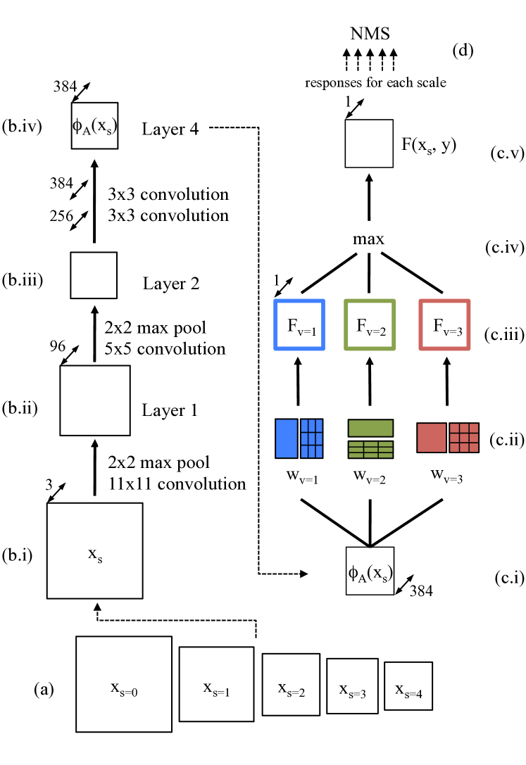
The architecture of our model is shown in Fig. 3. For a given input image $x$, we first construct an image pyramid (a) with five intervals over one octave We apply the ConvNet (b) at each scale $x_{s}$ to generate feature maps $\phi_{A}(x_{s})$. These are then passed to the DPM (c) for each class; as we describe in Section 3.2, the DPM may also be formulated as a series of neural network layers. At training time, the loss is computed using the final detection output obtained after NMS (d), and this is then back-propagated end-to-end through the entire system, including NMS, DPM and ConvNet.

3.1 Convolutional Network

We generate appearance features $\phi_{A}(x)$ using the first five layers of a Convolutional Network pre-trained for the ImageNet Classification task. We first train an eight layer classification model, which is composed of five convolutional feature extraction layers, plus three fully-connected classification layers. After this network has been trained, we throw away the three fully-connected layers, replacing them instead with the DPM. The five convolutional layers are then used to extract appearance features.

Note that for detection, we apply the convolutional layers to images of arbitrary size (as opposed to ConvNet training, which uses fixed-size inputs). Each layer of the network is applied in a bottom-up fashion over the entire spatial extent of the image, so that the total computation performed is still proportional to the image size. This stands in contrast to [7], who apply the ConvNet with a fixed input size to different image regions, and is more similar to [13].

Applying the ImageNet classification model to PASCAL detection has two scale-related problems that must be addressed. The first is that there is a total of 16x subsampling between the input and the fifth layer; that is, each pixel in $\phi_{A}$ corresponds to 16 pixels of input — this is insufficient for detection, as it effectively constrains detected bounding boxes to a lie on a 16-pixel grid. The second is that the ImageNet classifier was trained on objects that are fairly large, taking up much of the 224x224 image area. By contrast, many target objects in PASCAL are significantly smaller.

To address these, we simply apply the first convolution layer with a stride of 1 instead of 4 when combining with the DPM (however, we also perform 2x2 pooling after the top ConvNet layer due to speed issues in training, making the net resolution increase only a factor of 2). This addresses both scale issues simultaneously. The feature resolution is automatically increased by elimination of the stride. Moreover, the scale of objects presented to the network at layers 2 and above is increased by a factor of 4, better aligning the PASCAL objects to the ImageNet expected size This is due to the fact that when the second layer is applied to the output of the stride-1 maps, their field of view is 4x smaller compared to stride-4, effectively increasing the size of input objects.

Note that changing the stride of the first layer is effectively the same as upsampling the input image, but preserves resolution in the convolutional filters (if the filters were downsampled, these would be equivalent operations; however we found this to work well without changing the filter size, as they are already just 11x11).

3.2 Deformable Parts Model

3.2.1 Part Responses

The first step in the DPM formulation is to convolve the appearance features with the root and parts filters, producing appearance responses. Each object view has both a root filter and nine parts filters; the parts are arranged on a 3x3 grid relative to the root, as illustrated in Fig. 4. (This is similar to [19], who find this works as well as the more complex placements used by [5]). Note that the number of root and parts filters is the same for all classes, but the size of each root and part may vary between classes and views.

Given appearance filters $w_{A,y,v}^{\rm root}$ for each class $y$ and view $v$, and filters $w_{A,y,v,p}^{\rm part}$ for each part $p$, the appearance scores are:

$$F_{v}^{\rm root}(x_{s},y) = w_{A,y,v}^{\rm root}*\phi_{A}(x_{s})$$ (1)

$$F_{v,p}^{\rm part}(x_{s},y) = w_{A,y,v,p}^{\rm part}*\phi_{A}(x_{s})$$ (2)

Part responses are then fed to the deformation layer.

3.2.2 Deformation Layer

The deformation layer finds the optimal part locations, accounting for both apperance and a deformation cost that models the spatial relation of the part to the root. Given appearance scores $F_{v,p}^{\rm part}$, part location $p$ relative to the root, and deformation parameters $w_{D,v,p}$ for each part, the deformed part responses are the following (input variables $(x_{s},y)$ omitted):

$$F_{v,p}^{\rm def}=\max_{\delta_{i},\delta_{j}}~{}F_{v,p}^{\rm part}[p_{i}+\delta_{i},p_{j}+\delta_{j}]+w_{D,v,p}^{\rm part}\phi_{D}(\delta_{i},\delta_{j})$$ (3)

where $F_{v,p}^{\rm part}[p_{i}+\delta_{i},p_{j}+\delta_{j}]$ is the part response map $F_{v,p}^{\rm part}(x_{s},y)$ shifted by spatial offset $(p_{i}+\delta_{i},p_{j}+\delta_{j})$, and $\phi_{D}(\delta_{i},\delta_{j})=[|\delta_{i}|,|\delta_{j}|,\delta_{i}^{2},\delta_{j}^{2}]^{T}$ is the shape deformation feature. $w_{D,y,v}^{\rm part}\geq 0$ are the deformation weights.

Note the maximum in Eqn. 3 is taken independently at each output spatial location: i.e. for each output location, we find the max over possible deformations $(\delta_{i},\delta_{j})$. In practice, searching globally is unnecessary, and we constrain to search over a window $[-s,s]\times[-s,s]$ where $s$ is the spatial size of the part (in feature space). During training, we save the optimal $(\hat{\delta}_{i},\hat{\delta}_{j})$ at each output location found during forward-propagation to use during back-propagation.

The deformation layer extends standard max-pooling over $(\delta_{i},\delta_{j})$ with (i) a shift offset $(p_{i},p_{j})$ accounting for the part location, and (ii) deformation cost $w_{D}^{T}\phi_{D}(\delta_{i},\delta_{j})$. Setting both of these to zero would result in standard max-pooling.

(a) $w_{A,v}^{\rm root}$         (b) $w_{A,v}^{\rm part}$         (c) $w_{A,v}^{\rm part},w_{D,v}^{\rm part}$

Figure 4: Root and parts filter setup for our DPM. (a) Each view $v$ has a root filter with a different pre-defined aspect ratio. (b) Part filters are aligned on a 3x3 grid relative to the root. (c) Parts may deform relative to the root position at a cost, parameterized by $w_{D}^{\text{part}}$.

3.2.3 AND/OR Layer

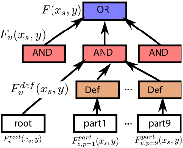
Combining the scores of root, parts and object views is done using an AND-like accumulation over parts to form a score $F_{v}$ for each view $v$, followed by an OR-like maximum over views to form the final object score $F$:

$$F_{v}(x_{s},y) = F^{\rm root}_{v}(x_{s},y)+\sum_{p\in{\rm parts}}F^{\rm def}_{v,p}(x_{s},y)$$ (4)

$$F(x_{s},y) = \max_{v\in{\rm views}}F_{v}(x_{s},y)$$ (5)

$F(x_{s},y)$ is then the final score map for class $y$ at scale $s$, given the image $x$ as shown in Fig. 5(left).

Figure 5: Left: Overview of the top part of our network architecture: (i) the root and part layers are convolution layers with different sizes of filter but same input size; (ii) OR/AND/Def layer preserve the size of the input to the output; (iii) each AND layer represents an object view which contains a root and 9 parts.
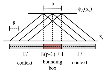
Right: Aligning a bounding box from DPM prediction through the convolutional network (see Section 3.3).

3.3 Bounding Box Prediction

After obtaining activation maps for each class at each scale of input, we trace the activation locations back to their corresponding bounding boxes in input space. Detection locations in $F(x_{s},y)$ are first projected back to boxes in $\phi_{A}(x_{s})$, using the root and parts filter sizes and inferred parts offsets. These are then projected back into input space through the convolutional network. As shown in Fig. 5(right), each pixel in $\phi_{A}(x_{s})$ has a field of view of 35 pixels in the input, and moving by 1 pixel in $\phi_{A}$ moves by 8 pixels in the input (due to the 8x subsampling of the convolutional model). Each bounding box is obtained by choosing the input region that lies between the field of view centers of the box’s boundary. This means that 17 pixels on all sides of the input field of view are treated as context, and the bounding box is aligned to the interior region.

3.4 Non-Maximal Suppression (NMS)

The procedure above generates a list of label assignments $A_{0}=\{(b_{i},y_{i},r_{i})_{i=1\dots|B|}\}$ for the image, where $b_{i}$ is a bounding box, and $y_{i}$ and $r_{i}$ are its associated class label and network response score, i.e. $r_{i}$ is equal to $F(x,y_{i})$ at the output location corresponding to box $b_{i}$. $B$ is the set of all possible bounding boxes in the search.

The final detection result is a subset of this list, obtained by applying a modified version of non-maximal suppression derived from [19]. If we label location $b_{i}$ as object type $y_{i}$, some neighbors of $b_{i}$ might also have received a high scores, where the neighbors of $b$ are defined as $neigh(b)=\{b^{\prime}|overlap(b,b^{\prime})\geq\theta\}$. However, $neigh(b_{i})\setminus b_{i}$ should not be labeled as $y_{i}$ to avoid duplicate detections. Applying this, we get a subset of $A=\{(b_{i},y_{i},r_{i})_{i=1\dots n}\}$ as the final detection result; usually $n\ll|B|$.

When calculating $overlap(b,b^{\prime})$, we use a symmetric form when the bounding boxes are for different classes, but an asymmetric form when the boxes are both of the same class. For different-class boxes, $overlap(b,b^{\prime})=\frac{Area(b\cap b^{\prime})}{Area(b\cup b^{\prime})}$, and threshold $\theta=0.75$. For same-class boxes, e.g. boxes of different views or locations, $overlap(b,b^{\prime})=\max\left(\frac{Area(b\cap b^{\prime})}{Area(b)},\frac{Area(b\cap b^{\prime})}{Area(b^{\prime})}\right)$ and $\theta=0.5$.

4 Final Prediction Loss

4.1 Motivation

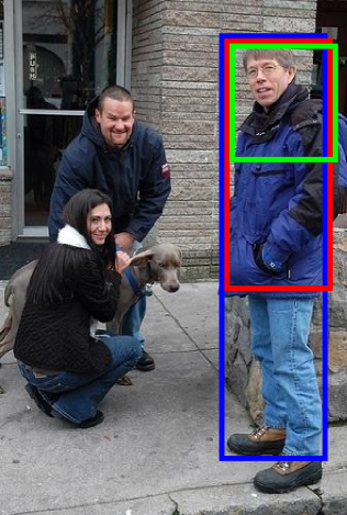
Our second main contribution is the use of a final-prediction loss that takes into account the NMS step used in inference. In contrast to bootstrapping with a hard negative pool, such as in [19] [5], we consider each image individually when determining positive and negative examples, accounting for NMS and the views present in the image itself. Consider the example in Fig. 6: A person detector may fire on three object views: red, green, and blue. The blue (largest in this example) is closest to the ground truth, while green and red are incorrect predictions. However, we cannot simply add the green or red boxes to a set negative examples, since they are indeed present in other images as occluded people. This leads to a situation where the red view has a higher inference score than blue or green, i.e. $r(red)>r(blue)$ and $r(red)>r(green)$, because red is never labeled as negative in the bootstrapping process. After NMS, blue response will be suppressed by red, causing a NMS error. Such an error can only be avoided when we have a global view on each image: if $r(blue)>r(red)$, then we would have a correct final prediction.

Figure 6: Three possible bounding boxes: blue, green and red (blue closest to the ground truth). However, green and red should not be considered negative instances (since they may be positive in other images where the person is occluded). Thus, we want
$r(blue)>r(red)$
$r(blue)>r(green)$

4.2 Loss Function

Recall that the NMS stage produces a set of assignments predicted by the model $A=\{(b_{i},y_{i},r_{i})_{i=1\dots n}\}$ from the set $B$ of all possible assignments. We compose the loss using two terms, $C(A)$ and $C(A^{\prime})$. The first, $C(A)$, measures the cost incurred by the assignment currently predicted by the model, while $C(A^{\prime})$ measures the cost incurred by an assignment close to the ground truth. The current prediction cost $C(A)$ is:

$$C(A)=\underbrace{\sum_{(b_{i},y_{i},r_{i})\in A}H(r_{i},y_{i})}_{C^{P}(A)}+\underbrace{\sum_{(b_{j},y_{j},r_{j})\in S(A)}H(r_{j},0)}_{C^{N}(A)}$$ (6)

where $H(r,y)=I(y>0)\max(0,1-r)^{2}+I(y=0)\max(0,r+1)$ i.e. a squared hinge error. $S(A)$ is the set of all bounding boxes predicted to be in the background ($y=0$): $S(A)=B\setminus neigh(A)$ with $neigh(A)=\bigcup_{(b_{i},y_{i},r_{i})\in A}neigh(b_{i})$. $C_{P}(A)$ and $C_{N}(A)$ are the set of positive predicted labels and the set of background labels, respectively.

The second term in the loss, $C(A^{\prime})$, measures the cost incurred by the ground truth bounding boxes under the model. Let the ground truth bounding box set be $A^{gt}=\{(b^{gt}_{i},y^{gt}_{i})_{i=1\dots m}\}$. We construct a constrained inference assignment $A^{\prime}$ close to $A^{gt}$ by choosing for each $b^{gt}_{i}$ the box $(b^{\prime}_{i},y^{\prime}_{i},r^{\prime}_{i})=\operatornamewithlimits{argmax}_{(b,y,r)}r$, where the $\operatornamewithlimits{argmax}$ is taken over all $overlap(b,b^{gt}_{i})\geq\theta^{\prime}$; that is, the box with highest response out of those with sufficient overlap with the ground truth. ($\theta^{\prime}=0.7$ in our experiments.) Similarly to before, the cost $C(A^{\prime})$ is:

$$C(A^{\prime})=\sum_{(b^{\prime}_{i},y^{\prime}_{i},r^{\prime}_{i})\in A^{\prime}}H(r^{\prime}_{i},y^{\prime}_{i})+\sum_{(b^{\prime}_{j},y^{\prime}_{j},r^{\prime}_{j})\in S(A^{\prime})}H(r^{\prime}_{j},0)$$ (7)

Thus we measure two costs: that of the current model prediction, and that of an assignment close to the ground truth. The final discriminative training loss is difference between these two:

$$L(A,A^{\prime})=C(A^{\prime})-C(A)\geq 0$$ (8)

Note this loss is always greater than 0 because the constrained assignment always has cost at least as large as the unconstrained one, and $L(A,A^{\prime})=0$ when $A=A^{\prime}$, i.e. when we produce detection results which are consistent with the ground truth $A^{gt}$.

Combining Equations 6 and 7 leads to

$$L(A,A^{\prime}) = L^{P}(A,A^{\prime})+L^{N}(A,A^{\prime})$$ (9)

$$L^{P}(A,A^{\prime}) = \sum_{(b^{\prime},y^{\prime},r^{\prime})\in A^{\prime}}H(r^{\prime},y^{\prime})-\sum_{(b,y,r)\in A}H(r,y)$$

$$L^{N}(A,A^{\prime}) = \sum_{(b^{\prime},y^{\prime},r^{\prime})\in S(A^{\prime})}H(r^{\prime},0)-\sum_{(b,y,r)\in S(A)}H(r,0)$$

$$= \sum_{(b,y,r)\in N\setminus N^{\prime}}H(r,0)-\sum_{(b^{\prime},y^{\prime},r^{\prime})\in N^{\prime}\setminus N}H(r^{\prime},0)$$

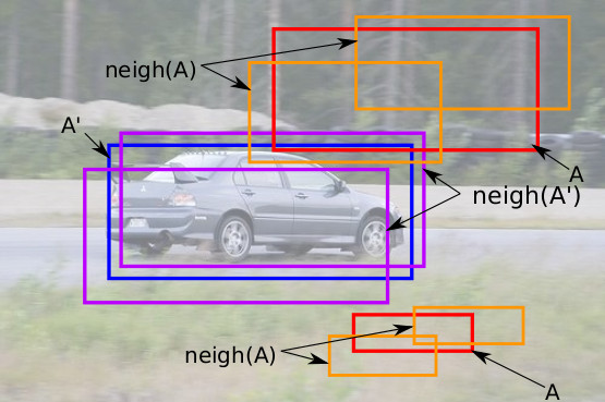
where $N=neigh(A)$ and $N^{\prime}=neigh(A^{\prime})$. The last line comes from the fact that most of the boxes included in $S(A)$ and $S(A^{\prime})$ are shared, and cancel out (see Fig. 7); thus we can compute the loss looking only at these neighborhood sets.

Figure 7: Illustration of ground-truth-constrained assignment $A^{\prime}$ and unconstrained assignments $A$ from the model, along with associated neighborhoods. Note neighborhoods are actually dense, and we show only a few boxes for illustration.

4.3 Interpretation and Effect on NMS Ordering

As mentioned earlier, a key benefit to training on the final predictions as we describe is that our loss accounts for the NMS inference step. In our example in Fig. 6, if the response $r(red)>r(blue)$, then $red\in A$ and $blue\in A^{\prime}$. Thus $L^{P}(A,A^{\prime})$ will decrease $r(red)$ and increase $r(blue)$. This ensures the responses $r$ are in an appropriate order when NMS is applied. Once $r(blue)>r(red)$, the mistake will be fixed.

The term $L^{N}$ in the loss is akin to an online version of hard negative mining, ensuring that the background is not detected as a positive example.

4.4 Soft Positive Assignments

When training jointly with the ConvNet, it is insufficient to measure the cost using only single positive instances, as the network can easily overfit to the individual examples. We address this using soft positive assignments in place of hard assignments; that is, we replace the definition of $C^{P}$ in Eqn. 6 used above with one using a weighted average of neighbors for each box in the assignment list:

$$C^{P}(A)=\sum_{b_{i}\in A}\frac{\sum_{b_{j}\in neigh(b_{i})}\alpha_{ij}H(r_{j},y_{j})}{\sum_{j}\alpha_{ij}}$$

where $\alpha_{ij}=2(Area(b_{i}\cap b_{j})/Area(b_{i}))-1$, and similarly for $C^{P}(A^{\prime})$.

Note a similar strategy has been tried in the case of HoG features before, but was not found to be beneficial [5]. By contrast, we found this to be important for integrating the ConvNet. We believe this is because the ConvNet has many more parameters than can easily overfit, whereas HoG is more constrained.

5 Training

Our model is trained in online fashion with SGD, with each image being forward propagated through the model and then the resulting error backpropagated to update the parameters. During the fprop, the position of the parts in the DPM are computed and then used for the subsequent bprop. Training in standard DPM models [5] differs in two respects: (i) a fixed negative set is mined periodically (we have no such set, instead processing each image in turn) and (ii) part positions on this negative set are fixed for many subsequent parameter updates.

We first pretrain the DPM root and parts filters without any deformation, using a fixed set of 20K random negative examples for each class. Note that during this stage, the ConvNet weights are fixed to their initialization from ImageNet. Following this, we perform end-to-end joint training of the entire system, including ConvNet, DPM and NMS (via the final prediction loss). During joint training, we use inferred part locations in the deformation layer.

The joint training phase is outlined in Algorithm 1. For each training image sample, we build an image pyramid, and fprop each scale of the pyramid through the ConvNet and DPM to generate the assignment list $A_{0}$. Note $A_{0}$ is represented using the output response maps. We then apply NMS to get the final assignments $A$, as well as construct the ground-truth constrained assignments $A^{\prime}$. Using the final prediction loss $L(A,A^{\prime})$ from Eqn. 9, we find the gradient and backpropagate through the network to update the model weights. We repeat this for 15 epochs through the training set with a learning rate $\eta=10^{-3}$, then another 15 using $\eta=10^{-4}$.

At test time, we simply forward-propagate the input pyramid through the network (ConvNet and DPM) and apply NMS.

Algorithm 1 Training algorithm for each image

1:  Input: Image $X$ with ground truth assignment $A^{gt}$

2:  Build image pyramid $X\rightarrow X_{1},X_{2},\dots,X_{s}$

3:  $A_{0}=\{\}$

4:  for  $X_{i}\in X_{1},X_{2},\dots X_{s}$ do

5:     $A_{0}=A_{0}\cup\mbox{assignments from responses~{}}F(X_{i};w)$

6:  end for

7:  find $A=NMS(A_{0})$

8:  find $A^{\prime}$ using $A_{0}$ and $A^{gt}$

9:  for  $X_{i}\in X_{1},X_{2},\dots X_{s}$ do

10:     find gradient at scale $i$: $g_{i}=\frac{\partial L(A,A^{\prime})}{\partial F(X_{i};w)}\frac{\partial F(X_{i};w)}{\partial w}$

11:  end for

12:  $w\leftarrow w+\eta\sum_{i}g_{i}$

6 Experiments

We apply our model to the PASCAL VOC 2007 and VOC 2011/2012 object detection tasks [4]. Table 1 shows how each component in our system improves performance on the PASCAL 2007 dataset. Our baseline implementation of HoG DPM with bootstrap training achieves 30.7 mAP. Switching HoG for a fixed pretrained ConvNet results in a large 32% relative performance gain to 40.8 mAP, corroborating the finding of [8] that such features greatly improve performance. On top of this, training using our online post-NMS procedure improves substantially improves performance to 43.3 mAP, and jointly training all components (ConvNet + DPM + NMS) further improves to 46.5 mAP.

	Bootstrap	NMS loss	NMS loss+FT
HoG-root	22.8	23.9	N/A
HoG-root+part	30.7	33.2	N/A
conv-root	38.7	40.3	43.1
conv-root+part	40.8	43.3	46.5

Table 1: A performance breakdown of our approach. Columns show different training methods and loss functions. Rows show different feature extractors and DPM with/without parts. Note: (i) conv features give a significant boost; (ii) our new NMS loss consistently improves performance, irrespective of features/model used and (iii) fine-tuning (FT) of the entire model gives further gains.

In addition, we can train different models to produce detections for each class, or train all classes at once using a single model with shared ConvNet feature extractor (but different DPM components). Training all classes together further boosts performance to 46.9% mAP. Note that this allows the post-NMS loss to account for objects of different classes as well as locations and views within classes, and also makes inference faster due to the shared features. We call this model “conv-dpm+FT-all”, and the separate-class set of models “conv-dpm+FT”.

Comparisons with other systems are shown in Tables 2 (VOC 2007) and 3 (VOC 2011/2012). For VOC 2007 (Table 2), our results are very competitive, beating all other methods except the latest version of R-CNN trained on $fc_{7}$ (“R-CNN(v4)FT $fc_{7}$”). Notably, we outperform the DP-DPM method ($45.2\%$ vs. our $46.9\%$), due to our integrated joint training and online NMS loss. In addition, our final model achieves comparible performance to R-CNN [7] with a similar feature extractor using $pool_{5}$ features ($46.9\%$ vs. $47.3\%$). Recent version of R-CNN achieve a better performance $54.2\%$ using a more complex network which includes fully connected layers ($fc_{7}$); extending our model to use deeper networks may also provide similar gains from better feature representations.

Table 3 shows our system performance on VOC2011. Here our system outperforms comparison methods, and in particular DP-DPM, achieving $43.7\%$ mAP versus $29.6\%$ for HoG-DPM [5] and $41.6\%$ for DP-DPM [8].

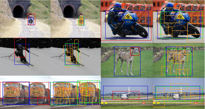
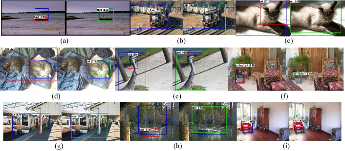
Finally, we provide examples of detections from our model in Figures 8, 9 and 10. Detection results are either show in green or red with ground truth bounding box in blue. Figure 10 illustrates training with our new loss function helps model fix problem for both inter-class and intra-class NMS. Our loss allows the larger view of the train to be selected in $(b)$, rather than the more limited view that appears in more images. However, the gains are not limited to selecting larger views: In $(d)$, we see a cat correctly selected at a smaller scale. Finally, there are also examples of inter-class correction in $(g)$, e.g. “train” being selected over “bus”.

Figure 8 shows the effect of using a DPM with parts over just the root-only model. Figures 9 shows correct and incorrect detection examples.

Figure 8: Examples of detections using root filter only (left half of each example; red) and the DPM with both root and part filters (right halves; green+orange).

7 Discussion

We have described an object detection system that integrates a Convolutional Network, Deformable Parts model and NMS loss in an end-to-end fashion. This fuses together aspects from both structured learning and deep learning: object structures are modeled by a composition of parts and views, while discriminative features are leveraged for appearance comparisons. Our evaluations show that our model achieves competitive performance on PASCAL VOC 2007 and 2011 datasets, and achieves substantial gains from integrating both ConvNet features as well as NMS, and training all parts jointly.

VOC2007	aero	bike	bird	boat	botl	bus	car	cat	chair	cow	table	dog	horse	mbike	pers	plant	sheep	sofa	train	tv	mAP
DetectorNet [14]	29.2	35.2	19.4	16.7	3.7	53.2	50.2	27.2	10.2	34.8	30.2	28.2	46.6	41.7	26.2	10.3	32.8	26.8	39.8	47.0	30.5
HoG-dpm(v5) [5]	33.2	60.3	10.2	16.1	27.3	54.3	58.2	23.0	20.0	24.1	26.7	12.7	58.1	48.2	43.2	12.0	21.1	36.1	46.0	43.5	33.7
HSC-dpm [12]	32.2	58.3	11.5	16.3	30.6	49.9	54.8	23.5	21.5	27.7	34.0	13.7	58.1	51.6	39.9	12.4	23.5	34.4	47.4	45.2	34.3
Regionlets [17]	54.2	52.0	20.3	24.0	20.1	55.5	68.7	42.6	19.2	44.2	49.1	26.6	57.0	54.5	43.4	16.4	36.6	37.7	59.4	52.3	41.7
DP-DPM [8]	44.6	65.3	32.7	24.7	35.1	54.3	56.5	40.4	26.3	49.4	43.2	41.0	61.0	55.7	53.7	25.5	47.0	39.8	47.9	59.2	45.2
R-CNN [7]$fc_{7}$	56.1	58.8	34.4	29.6	22.6	50.4	58.0	52.5	18.3	40.1	41.3	46.8	49.5	53.5	39.7	23.0	46.4	36.4	50.8	59.0	43.4
R-CNN(v1)FT $pool_{5}$	55.6	57.5	31.5	23.1	23.2	46.3	59.0	49.2	16.5	43.1	37.8	39.7	51.5	55.4	40.4	23.9	46.3	37.9	49.7	54.1	42.1
R-CNN(v4)FT $pool_{5}$	58.2	63.3	37.9	27.6	26.1	54.1	66.9	51.4	26.7	55.5	43.4	43.1	57.7	59.0	45.8	28.1	50.8	40.6	53.1	56.4	47.3
R-CNN(v1)FT $fc_{7}$	60.3	62.5	41.4	37.9	29.0	52.6	61.6	56.3	24.9	52.3	41.9	48.1	54.3	57.0	45.0	26.9	51.8	38.1	56.6	62.2	48.0
R-CNN(v4)FT $fc_{7}$	64.2	69.7	50.0	41.9	32.0	62.6	71.0	60.7	32.7	58.5	46.5	56.1	60.6	66.8	54.2	31.5	52.8	48.9	57.9	64.7	54.2
HoG	29.3	55.5	9.3	13.3	25.2	43.1	53	20.4	18.5	25.1	23.3	10.3	55.4	44.2	40.8	10.5	19.8	34.3	43.3	39.5	30.7
HoG+	32.8	58.5	10.3	16.0	27.1	46.1	56.9	21.9	20.6	27.2	26.4	13.0	57.8	47.5	44.2	11.0	22.7	36.5	45.8	42.1	33.2
conv-root	38.1	60.9	21.9	17.8	29.3	51.4	58.5	26.7	16.5	31.1	33.2	24.2	65.0	58.0	44.4	21.7	35.4	36.8	49.5	54.1	38.7
conv-dpm	45.3	64.5	21.1	21.0	34.2	54.4	59.0	32.6	20.0	31.0	34.5	25.3	63.8	60.1	45.0	23.2	36.0	38.4	51.5	56.2	40.8
conv-dpm+	48.9	67.3	25.3	25.1	35.7	58.3	60.1	35.3	22.7	36.4	37.1	26.9	64.9	62.0	47.0	24.1	37.5	40.2	54.1	57.0	43.3
conv-dpm+ FT	50.9	68.3	31.9	28.2	38.1	61.0	61.3	39.8	25.4	46.5	47.3	29.6	67.5	63.4	46.1	25.2	39.1	45.4	57.0	57.9	46.5
conv-dpm+ FT-all	49.3	69.5	31.9	28.7	40.4	61.5	61.5	41.5	25.5	44.5	47.8	32.0	67.5	61.8	46.7	25.9	40.5	46.0	57.1	58.2	46.9

Table 2: Mean AP on PASCAL VOC 2007

VOC2011/2012	aero	bike	bird	boat	botl	bus	car	cat	chair	cow	table	dog	horse	mbike	pers	plant	sheep	sofa	train	tv	mAP
HoG-DPM [5]	45.6	49.0	11.0	11.6	27.2	50.5	43.1	23.6	17.2	23.2	10.7	20.5	42.5	44.5	41.3	8.7	29.0	18.7	40.0	34.5	29.6
conv-root	56.0	45.4	20.6	12.7	29.5	49.2	38.6	38.1	16.4	28.2	22.9	28.8	48.3	52.1	47.7	17.0	39.1	29.6	41.2	48.6	35.5
conv-dpm	56.9	53.2	26.6	17.6	29.9	51.4	42.5	42.4	16.5	31.6	25.0	37.7	52.7	56.7	49.9	16.5	41.0	30.9	44.4	49.7	38.4
conv-dpm+	59.6	56.6	29.8	20	31.1	55.8	42.8	43.3	18.3	35.6	28.5	39.7	56.3	59.7	51.1	19.6	42.1	33.1	49.1	50.3	41.1
conv-dpm+FT-all	63.3	60.2	33.4	24.4	33.6	60	44.7	49.3	19.4	36.6	30.2	40.7	57.7	61.4	52.3	21.2	44.4	37.9	51.1	52.2	43.7

Table 3: Mean AP on PASCAL VOC 2011

Figure 9: Examples of correct (green) and incorrect (red) detections found by our model.

Figure 10: Examples of model with (green) and without (red) NMS loss (parts location are ommited)

References

- [1] Y. Chen, L. Zhu, and A. L. Yuille. Active mask hierarchies for object detection. In ECCV 2010, volume 6315 of Lecture Notes in Computer Science, pages 43–56. Springer, 2010.
- [2] N. Dalal and B. Triggs. Histograms of oriented gradients for human detection. In CVPR, 2005.
- [3] C. Desai, D. Ramanan, and C. Fowlkes. Discriminative models for multi-class object layout. International Journal of Computer Vision, 2011.
- [4] M. Everingham, L. Van Gool, C. K. I. Williams, J. Winn, and A. Zisserman. The PASCAL Visual Object Classes Challenge 2012 (VOC2012) Results.
- [5] P. F. Felzenszwalb, R. B. Girshick, D. McAllester, and D. Ramanan. Object detection with discriminatively trained part-based models. IEEE Trans. Pattern Anal. Mach. Intell., 32(9):1627–1645, Sept. 2010.
- [6] P. F. Felzenszwalb, R. B. Girshick, D. McAllester, and D. Ramanan. Object detection with discriminatively trained part based models. IEEE Transactions on Pattern Analysis and Machine Intelligence, 32(9):1627–1645, 2010.
- [7] R. B. Girshick, J. Donahue, T. Darrell, and J. Malik. Rich feature hierarchies for accurate object detection and semantic segmentation. CoRR, abs/1311.2524, 2013.
- [8] R. B. Girshick, F. N. Iandola, T. Darrell, and J. Malik. Deformable part models are convolutional neural networks. CoRR, abs/1409.5403, 2014.
- [9] A. Krizhevsky, I. Sutskever, and G. E. Hinton. Imagenet classification with deep convolutional neural networks. pages 1106–1114, 2012.
- [10] Y. LeCun, L. Bottou, Y. Bengio, and P. Haffner. Gradient-based learning applied to document recognition. Proceedings of the IEEE, 86(11):2278 –2324, nov 1998.
- [11] D. Parikh and C. L. Zitnick. Human-debugging of machines. In In NIPS WCSSWC, 2011.
- [12] X. Ren and D. Ramanan. Histograms of sparse codes for object detection. 2013 IEEE Conference on Computer Vision and Pattern Recognition, 0:3246–3253, 2013.
- [13] P. Sermanet, D. Eigen, X. Zhang, M. Mathieu, R. Fergus, and Y. LeCun. Overfeat: Integrated recognition, localization and detection using convolutional networks. CoRR, abs/1312.6229, 2013.
- [14] C. Szegedy, A. Toshev, and D. Erhan. Deep neural networks for object detection. NIPS, 2013.
- [15] J. Tompson, A. Jain, Y. LeCun, and C. Bregler. Joint training of a convolutional network and a graphical model for human pose estimation. CoRR, abs/1406.2984, 2014.
- [16] J. Uijlings, K. Sande, T. Gevers, and A. Smeulders. Selective search for object recognition. International Journal of Computer Vision, 104(2):154–171, 2013.
- [17] X. Wang, M. Yang, S. Zhu, and Y. Lin. Regionlets for generic object detection. IEEE 14th International Conf. on Computer Vision, 2013.
- [18] M. D. Zeiler and R. Fergus. Visualizing and understanding convolutional networks. CoRR, abs/1311.2901, 2013.
- [19] L. L. Zhu, Y. Chen, A. Yuille, and W. Freeman. Latent hierarchical structural learning for object detection. 2010 IEEE Conference on Computer Vision and Pattern Recognition, 0:1062–1069, 2010.