Using Graphics Processing Units to solve the classical $N$-Body Problem in Physics and Astrophysics

Abstract

Graphics Processing Units (GPUs) can speed up the numerical solution of various problems in astrophysics including the dynamical evolution of stellar systems; the performance gain can be more than a factor 100 compared to using a Central Processing Unit only. In this work I describe some strategies to speed up the classical $N$-body problem using GPUs. I show some features of the $N$-body code HiGPUs as template code. In this context, I also give some hints on the parallel implementation of a regularization method and I introduce the code HiGPUs-R. Although the main application of this work concerns astrophysics, some of the presented techniques are of general validity and can be applied to other branches of physics such as electrodynamics and QCD.

1 Introduction

The $N$-body problem is the study of the motion of $N$ point-like particles interacting through their mutual forces that can be expressed according to a specific physical law. In particular, if the reciprocal interaction is well approximated by the Newton’s gravity law, we refer to the classical, gravitational $N$-body problem. The differential equations that describe the kinematics of the $N$-body system are

$$\begin{cases}\mathbf{\ddot{r}}_{i}&=-G\sum\limits_{\begin{subarray}{c}j=1\\ j\neq i\end{subarray}}^{N}\frac{m_{j}}{{r_{ij}}^{3}}\mathbf{r_{ij}}\\ \mathbf{r}_{i}\left(t_{0}\right)&={\mathbf{r}}_{i,0}\hskip 50.0pti=1,2,...,N\\ \mathbf{\dot{r}}_{i}\left(t_{0}\right)&={\mathbf{\dot{r}}}_{i,0}\end{cases}$$ (1)

where $t$ is the time, $\mathbf{r}_{i}$, $\mathbf{\dot{r}}_{i}$ and $\mathbf{\ddot{r}}_{i}$ are the position, the velocity and the acceleration of the $i$-th particle, respectively, $G$ is the universal gravitational constant, $m_{j}$ indicates the mass of the particle $j$, ${\mathbf{r}}_{i,0}$ and ${\mathbf{\dot{r}}}_{i,0}$ represent the initial position and velocity and $r_{ij}$ is the mutual distance between particle $i$ and particle $j$. Although we know that the solution of the system of equations (1) exists and is unique, we do not have its explicit expression. Therefore, the best way to solve the $N$-body problem is numerical. The numerical solution of the system of equations (1) is considered a challenge despite the considerable advances in both software development and computing technologies; for instance, it is still not possible to study the dynamical evolution of stellar systems composed of more than $\sim 10^{6}$ objects without the need of theoretical approximations. The numerical issues come mainly from two aspects:

• ultraviolet divergence (UVd): close encounters between particles ($r_{ij}\rightarrow 0$) produce a divergent mutual force ($F_{ij}\rightarrow\infty$). The immediate consequence is that the numerical time step must be very small in order to follow the rapid changes of positions and velocities with sufficient accuracy, slowing down the integration.

• infrared divergence (IRd): to evaluate the acceleration of the $i$-th particle we need to take into account all the other $N-1$ contributions because the gravitational force never vanishes ($F_{ij}\rightarrow 0\Leftrightarrow r_{ij}\rightarrow\infty$). This implies that the $N$-body problem has a computational complexity of $O\left(N^{2}\right)$.

To control the effects of the UVd and smooth the behavior of the force during close encounters, a parameter $\epsilon$ (softening parameter) is introduced in the gravitational potential. This leads to an approximate expression for the reciprocal attraction which is

$$\mathbf{F_{i}}=-G\frac{m_{i}m_{j}}{\left({r_{ij}}^{2}+\epsilon^{2}\right)^{\tfrac{3}{2}}}\mathbf{r_{ij}}.$$ (2)

In this way, the UVd is artificially removed paying a loss of resolution at spatial scales comparable to $\epsilon$ and below. An alternative approach concerns the usage of a regularization method, that is a coordinate transformation that modifies the standard $N$-body Hamiltonian removing the singularity for $r_{ij}=0$. We briefly discuss this strategy in Sec. 3.

On the other hand, the issues that come from the IRd can be overcome using:

1. approximation schemes: the direct sum of inter-particle forces is replaced by another mathematical expression with lower computational complexity. To this category belongs, for instance, the tree scheme, originally introduced by Barnes and Hut, which is one of the most known approximation strategies [1];

2. hardware acceleration: it is also possible to use more efficient hardware to speed up the force calculation maintaining the $O\left(N^{2}\right)$ computational complexity of the problem.

For what concerns hardware advances, Graphics Processing Units (GPUs) can act as computing accelerators of the evaluation of the mutual forces. This approach is extremely efficient because a GPU is a highly parallel device which can have up to $\sim$ 3,000 cores and run up to $\sim$ 80,000 virtual units (GPU threads) that can execute independent instructions at the same time. Since the evaluations of mutual distances can be executed independently, a GPU perfectly matches the structure of the $N$-body problem. Nowadays, the overwhelming majority of $N$-body simulations are carried out exploiting the GPU acceleration.

2 The direct $N$-body code HiGPUs

In this section I give an overview of the most common strategies adopted to numerically solve the $N$-body problem using a GPU. I describe the HiGPUs code as an example of GPU optimized $N$-body code [2]. HiGPUs is a direct summation $N$-body code that implements a Hermite 6th order time integrator. It is written combining utilities of C and C++ and it uses CUDA (or OpenCL), MPI and OpenMP to exploit GPU workstations as well as GPU clusters. The main features of HiGPUs and of other GPU optimized $N$-body codes are the following:

1. THE HERMITE ALGORITHM: the Hermite time integrators (4th, 6th and 8th order) represent the state of the art of direct $N$-body simulations( [4], [3]). In particular, the 4th order scheme is, by far, the most widely used algorithm in this context being particularly efficient in terms of ratio between computing time and accuracy. The Hermite integrators are based on Taylor series of positions and velocities and their most important feature is that they have high accuracy even though they need to evaluate the distances between particles just once per time step. This is a huge advantage in using Hermite integrators if we consider that, for example, a standard Runge-Kutta method needs to evaluate accelerations 4 times per integration step and it is “only” 4th order accurate.

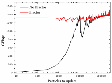
Figure 1: The effects of the Bfactor optimization on the performance of a GeForce GTX TITAN Black (measured in billions of floating point operations per second, GFlops) as a function of the number of particles that need to be updated (according to the block time steps distribution). The results were obtained using the $N$-body code HiGPUs with $N\simeq 260,000$.

2. BLOCK TIME STEPS: stars in an $N$-body system can have very different accelerations; this corresponds to have a large variety of evolutionary time-scales. In this context, it is convenient to assign to all the objects their own time step which becomes a function of the physical parameters that describe the kinematic state of the corresponding particle. In order to avoid time synchronization issues among the $N$ bodies and to simplify the parallelization process, the time step is forced to be a power of two. Thus, particles are sub-divided in several groups (blocks) that share the same time step [4]. In this way we need to update positions and velocities only of $m\leq N$ particles per time step; in particular, bodies with smaller time steps will be updated more often than particles with bigger time steps for which the kinematic state will be estimated using Taylor expansions only. This implies that the computational complexity per time step is reduced from $O\left(N^{2}\right)$ to $O\left(mN\right)$.

3. THE Bfactor VARIABLE: another important aspect concerns the GPU load. For example, a GeForce GTX TITAN Black GPU can run a maximum of 30,720 threads in parallel, therefore we need to fittingly distribute the work load to fully exploit this kind of GPU. When using the block time steps strategy it is quite common to have $m<30,720$ therefore we introduce the variable Bfactor that can increase the number of running threads and further split and distribute the work load among the GPU cores. For instance, if we have $m<30,720$ and Bfactor$=B$ we run $mB$ threads and each thread calculates the accelerations due to $N/B$ bodies. The optimal Bfactor value must be determined step by step. We show in Fig. 1 the differences in terms of GPU performance running a typical $N$-body simulation with and without the Bfactor variable. It is evident that, for a GeForce GTX TITAN Black, when the particles that must be updated are $m\lesssim 30,720$ we obtain significantly higher performance when the Bfactor optimization is turned on. A similar optimization strategy can be found in [5].

4. PRECISION: it is well known that the maximum theoretical performance of all the GPUs in double precision (DP) is lower than their capability to execute single precision (SP) operations. For $N$-body problems it is important to use DP to calculate reciprocal distances and to cumulate accelerations in order to reduce round-off errors as much as possible. All the other instructions (square roots included) can be executed in SP to speed up the integration. Some authors use an alternative approach based on an emulated double precision arithmetic (also known as double-single precision or simply DS). In this strategy a DP variable is replaced with two, properly handled, SP values; in this way only SP quantities are used against a slightly larger number of operations that must be executed [6].

5. SHARED MEMORY: the GPU shared memory (SM) is a limited amount of memory (in general $\lesssim 65$kB) and it is shared between all the GPU threads in the same block and can be used for fast data transactions (on average, SM is about 10 times faster than “standard” memory). During the evaluation of the $N$-body accelerations, the best strategy is to cyclically load SM until all the pair-wise forces are computed.

2.1 Performance results

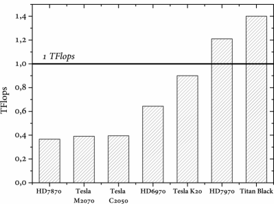
Figure 2: Left panel: speed up of the code HiGPUs as a function of the number of used GPUs for different $N$-body systems with $3.2\times{10^{4}}\lesssim N\lesssim 8\times{10^{6}}$. The dashed line corresponds to the maximum computing efficiency (linear speedup). Right panel: performance (in TFlops) of HiGPUs running on single, different GPUs. For the scalability tests we used the IBM DataPlex DX360M3 Linux Infiniband Cluster provided by the Italian supercomputing consortium CINECA.

Fig. 2 shows the scalability of the code HiGPUs on a GPU cluster (left panel) and its performance using single, different GPUs (right panel). Form Fig. 2, it is apparent that GPUs are extremely well suited to solve the $N$-body problem: we reach a computing efficiency of $\sim 92\%$ using 256 GPUs and $\sim 8$ million bodies and a sustained performance of $\sim 1.4$ TFlops on just one GPU (GeForce GTX TITAN Black). More details can be found in [2] and [7].

3 Regularization

Close encounters between (two or more) particles are critical in $N$-body simulations because of the UVd of the gravitational force. An attempt to remove the small-scale singularity of the interaction potential is referred as an attempt of regularization. The Burdet-Heggie method ( [8], [9]), the Kustaanheimo-Stiefel algorithm [10] or the Mikkola’s algorithmic formulation (MAR, [11]) are some of the most famous examples of regularization. In general, all these methods are quite expensive in terms of implementation effort and computing time but, if we use them to integrate few bodies only, they become both faster and much more accurate than standard $N$-body integrators. It is not convenient to implement regularization methods on a GPU because of their mathematical construction and because they can integrate, in general, a maximum of few tens of bodies. Nevertheless, during the dynamical evolution of an $N$-body system, we can identify the groups of particles that are in tight systems or that are experimenting a close encounter, and regularize them.

Figure 3: Left panel: trajectories obtained for the modified version of the Pythagorean 3-body problem, where the three particles are replaced with three binaries, using a regularized algorithm. Three binary systems, indicated with (1,2), (3,4) and (5,6), are initially placed at the vertices of a right triangle with null velocities. During the dynamical evolution, the particles 1, 2, 3 and 6 are ejected form the system with high velocities (outside directions are indicated with arrows) while particles 4 and 5 form a very hard binary. Right panel: relative energy variation during the integration of the Pythagorean problem.

This process can be done in parallel by the CPU, by means of OpenMP, establishing a 1 to 1 correspondence between groups that must be regularized and CPU threads. At the same time, given that the GPU kernels are asynchronous, the regularization process can be performed while the GPU works in background. This describes the parallel scheme adopted to implement the MAR in the code HiGPUs-R which is still under development. A test application to demonstrate the advantages of regularization is shown in Fig. 3. It represents a modified version of the so called Pythagorean 3-body problem (e.g. [12]) integrated with HiGPUs-R. Standard $N$-body integrators, such as the Hermite 4th order scheme, cannot evolve this system, because either the time step becomes prohibitively small throughout the dynamical evolution, or, if we fix a minimum time step, the solution is completely inaccurate. The only chance is to use a regularized code which is very fast ($\sim 10$ seconds of simulations to obtain the trajectories in the left panel of Fig. 3) and maintains a very good total energy conservation (see the right panel of Fig. 3).

4 Conclusions

In this work I have presented and discussed the main strategies adopted to speed up the numerical solution of the $N$-body problem using GPUs. I have also shown the main advantages in using regularization methods and described a new parallel scheme to implement the Mikkola’s algorithmic regularization in the context of a GPU $N$-body code. I have used the direct $N$-Body code HiGPUs as reference and I have given an overview of the code HiGPUs-R that is a new regularized version of HiGPUs. The development of fast and regularized $N$-body codes such as HiGPUs-R is of fundamental importance to investigate a large number of astrophysical problems (ranging from the dynamical evolution of star clusters to the formation of double black hole binaries).

5 Acknowledgments

MS thanks Michela Mapelli and Roberto Capuzzo Dolcetta for useful discussions, and acknowledges financial support from the MIUR through grant FIRB 2012 RBFR12PM1F.

References

- [1] J. Barnes and P. Hut, Nature 324 446 (1986)
- [2] R. Capuzzo-Dolcetta, M. Spera and D. Punzo, JCP 236 580 (2013)
- [3] Nitadori, K., & Makino, J., New Astronomy 13 498 (2008)
- [4] S.J. Aarseth, Gravitational N-body simulations: tools and algorithms, Cambridge Univ. Press, UK (2003)
- [5] L. Nyland, M. Harris and J. Prins, GPU gems 3 31 677 (2007)
- [6] E. Gaburov, S. Harfst and S. Portegies Zwart, New. Ast. 14 630 (2009)
- [7] R. Capuzzo-Dolcetta, M. Spera, Comp. Phys. Comm. 184 2528 (2013)
- [8] C.A. Burdet, Z. Angew. Math. Phys. 18 434 (1967)
- [9] D.C. Heggie, Astr. and Space Science Lib. 39 34 (1973)
- [10] P. Kustaanheimo and E. Stiefel, Jour. für Reine und Angew. Math. 218 204 (1965)
- [11] S. Mikkola and K. Tanikawa, Celest. Mech. Dyn. Astr. 74 287 (1999)
- [12] S. Mikkola and S.J. Aarseth, Celest. Mech. Dyn. Astr. 57 439 (1993)