CL²QCD - Lattice QCD based on OpenCL

Abstract:

We present the Lattice QCD application CL²QCD, which is based on OpenCL and can be utilized to run on Graphic Processing Units as well as on common CPUs. We focus on implementation details as well as performance results of selected features. CL²QCD has been successfully applied in LQCD studies at finite temperature and density and is available at .

1 Lattice QCD at Finite Temperature

Lattice QCD (LQCD) successfully describes many aspects of the strong interactions and is the only method available to study QCD from first principles. The idea is to discretize space-time on a $N_{\sigma}^{3}\times N_{\tau}$ hypercube with lattice spacing $a$ and treat this system with numerical methods. State-of-the-art lattice simulations require high-performance computing and constitute one of the most compute intensive problems in science. The discretization procedure is not unique and several different lattice theories of QCD have been developed. It is important, in general, to cross check each result using different formulations.

The QCD phase diagram is of great interest both theoretically and experimentally, e.g. at the dedicated programs at RHIC at Brookhaven, LHC at CERN or at the future FAIR facility in Darmstadt. On the lattice, studies at finite temperature $T$ are possible via the identification $T=(a(\beta)N_{\tau})^{-1}$. Thus, scans in $T$ require simulations at multiple values of the lattice coupling $\beta$. In addition, to employ a scaling analysis, simulations on various spatial volumes $N_{\sigma}^{3}$ are needed (to avoid finite size effects one typically uses $N_{\sigma}/N_{\tau}\approx 3$). Hence, studies at finite $T$ naturally constitute a parallel simulation setup. Currently, these investigations are restricted to zero chemical potential $\mu$, as the sign-problem prevents direct simulations at $\mu>0$. To circumvent this issue one can use reweighting, a Taylor series approach or one can employ a purely imaginary chemical potential $\mu_{I}$.

On the lattice, observables are evaluated by means of importance sampling methods by generating ensembles of gauge configurations $\{U_{m}\}$ using as probability measure the Boltzmann-weight $p[U,\phi]=\exp\left\{-S_{\text{eff}}[U,\phi]\right\}$. Expectation values are then

$$\left<K\right>\approx\frac{1}{N}\sum_{m}K[U_{m}]\;.$$

These ensembles are commonly generated using the Hybrid-Monte-Carlo (HMC) algorithm [1], which does not depend on any particular lattice formulation of QCD.

The fermions enter in the effective action $S_{\text{eff}}$ via the fermion determinant $\det D$, which is evaluated using pseudo-fermions $\phi$, requiring the inverse of the fermion matrix, $D^{-1}$. The fermion matrix $D$ is specific to the chosen discretization. The most expensive ingredient to current LQCD simulations is the inversion of the fermion-matrix

$$D\phi=\psi\quad\Rightarrow\quad\phi=D^{-1}\;\psi\;,$$

which is carried out with Krylov subspace methods, e.g. conjugate gradient (CG). During the inversion, the matrix-vector product $D\phi$ has to be carried out multiple times. The performance of this operation, like almost all LQCD operations, is limited by the memory bandwidth. For example, in the Wilson formulation, the derivative part of $D$, the so-called ${\not}D$, requires to read and write 2880 Bytes per lattice site in each call, while it performs only 1632 FLOPs per site, giving a rather low numerical density $\rho$ (FLOPs per Byte) of $\sim 0.57$. In the standard staggered formulation, the situation is even more bandwidth-dominated. To apply the discretization of the Dirac operator on a fermionic field ($D_{KS}\;\phi$) 570 FLOPs per each lattice site are performed and 1584 Bytes are read or written, with a consequent smaller $\rho$ of $\sim 0.35$. This emphasizes that LQCD requires hardware with a high memory-bandwidth to run effectively, and that a meaningful measure for the efficiency is the achieved bandwidth. In addition, LQCD functions are local, i.e. they depend on a number of nearest neighbours only. Hence, they are very well suited for parallelization.

2 OpenCL and Graphic Cards

	Chip	Peak SP	Peak DP	Peak BW
		{GFLOPS}	{GFLOPS}	{GB/s}
AMD Radeon HD 5870	Cypress	2720	544	154
AMD Radeon HD 7970	Tahiti	3789	947	264
AMD FirePro S10000	Tahiti	2$\times$3410	2$\times$850	2$\times$240
NVIDIA GeForce GTX 680	Kepler	3090	258	192
NVIDIA Tesla K40	Kepler	4290	1430	288
AMD Opteron 6172	Magny-Cours	202	101	43
Intel Xeon E5-2690	Sandy Bridge EP	371	186	51

Table 1: Theoretical peak performance of current GPUs and CPUs. SP and DP denote single and double precision, respectively. BW denotes bandwidth.

	LOEWE -CSC		SANAM
GPU nodes	600	40	304
GPUs/node	1 $\times$ AMD 5870	2 $\times$ AMD S10000	2 $\times$ AMD S10000
CPUs/node	2 $\times$ Opteron 6172	2 $\times$ Intel Xeon E5-2630 v2	2 $\times$ Xeon E5-2650

Table 2: AMD based clusters where CL²QCD was used for production runs.

Graphics Processing Units (GPUs) surpass CPUs in peak performance as well as in memory bandwidth (see Table 1) and can be used for general purposes. Hence, many clusters are today accelerated by GPUs, for example LOEWE -CSC in Frankfurt [2] or SANAM [3] (see Table 2). GPUs constitute an inherently parallel architecture. As LQCD applications are always memory-bandwidth limited (see above) they can benefit from GPUs tremendously. Accordingly, in recent years the usage of GPUs in LQCD simulations has increased. These efforts mainly rely on CUDA as computing language, applicable to NVIDIA hardware only. A hardware independent approach to GPU applications is given by the Open Computing Language (OpenCL), which is an open standard to perform calculations on heterogeneous computing platforms. This means that GPUs and CPUs can be used together within the same framework, taking advantage of their synergy and resulting in a high portability of the software. First attempts to do this in LQCD have been reported in [4].

An OpenCL application consists of a host program coordinating the execution of the actual functions, called kernels, on computing devices (Figure 1), like for instance GPUs or a CPUs.

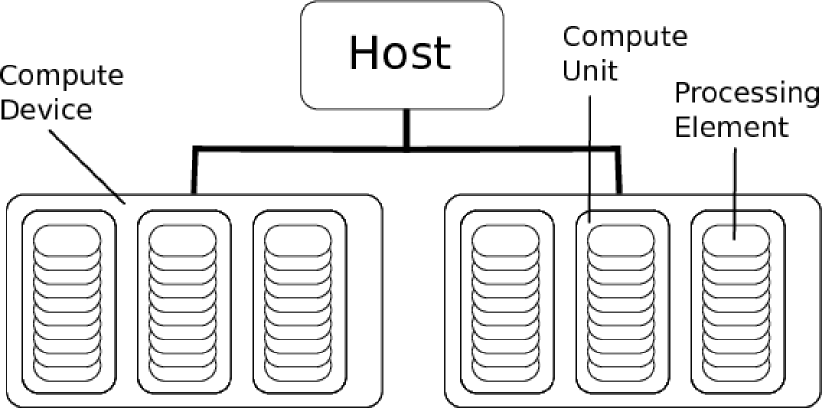
Figure 1: OpenCL concept

Although the hardware has different characteristics, GPU programming shares many similarities with parallel programming of CPUs. A computing device consists of multiple compute units. When a kernel is executed on a computing device, actually a huge number of kernel instances is launched. They are mapped onto work-groups consisting of work-items. The work-items are guaranteed to be executed concurrently only on the processing elements of the compute unit (and share processor resources on the device).

Compared to the main memory of traditional computing systems, on-board memory capacities of GPUs are low, though increasing more and more. This constitutes a clear boundary for simulation setups. Also, communication between host system and GPU is slow, limiting workarounds in case the available GPU memory is exceeded. Nevertheless, as finite $T$ studies are usually carried out on moderate lattice sizes (in particular $N_{\sigma}\gg N_{\tau}$), this is less problematic for the use cases CL²QCD was developed for.

3 CL²QCD Features

CL²QCD is a Lattice QCD application based on OpenCL, applicable to CPUs and GPUs. Focusing on Wilson fermions, it constitutes the first such application for this discretization type [5]. In particular, the so-called Twisted Mass Wilson fermions [6, 7], which ensure $\mathcal{O}(a)$ improvement at maximal twist, are implemented. Recently, the (standard) formulation of staggered fermions has been added. Improved gauge actions and standard inversion and integration algorithms are available, as well as ILDG-compatible IO and the RANLUX Pseudo-Random Number Generator (PRNG) [8]. More precisely, CL²QCD provides the following executables.

• HMC: Generation of gauge field configurations for $N_{f}=2$ Twisted Mass Wilson type or pure Wilson type fermions using the HMC algorithm [1].

• RHMC: Generation of gauge field configurations for $N_{f}$ staggered type fermions using the Rational HMC algorithm [9].

• SU3HEATBATH: Generation of gauge field configurations for $SU(3)$ Pure Gauge Theory using the heatbath algorithm [10, 11, 12].

• INVERTER: Measurements of fermionic observables on given gauge field configurations.

• GAUGEOBSERVABLES: Measurements of gauge observables on given gauge field configurations.

4 CL²QCD Code Structure

The host program of CL²QCD is set up in C++, which allows for independent program parts using C++ functionalities and also naturally provides extension capabilities. Cross-platform compilation is provided using the CMake framework.

The code structure of CL²QCD is displayed in Figure 2. It is separated in two main components: the physics package, representing high-level functionality, and the hardware package, representing low-level functionality. In addition, the meta package collects what is needed to control the program execution and IO operations.

All parts of the simulation code are carried out using OpenCL kernels in double precision. The OpenCL language is based on C99. In particular, concrete implementations of basic LQCD functionality like matrix-matrix multiplication, but also more complex operations like the ${\not}D$ or the (R)HMC force calculation, are found in the kernel files. Their compilation and execution is handled within the hardware package. The kernels are in a certain way detached from the host part as the latter can continue independently of the status of the kernel execution. This nicely shows the separation into the administrative part (host) and the performance-critical calculations (kernels).

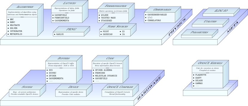
Figure 2: CL²QCD code structure. Packages and substructures are realized as namespaces. The names of the various components are, for the sake of simplicity, not always identical to those in the code.

The physics package provides representations of the physical objects like gauge fields or fermion fields. In addition, the corresponding classes provide functionality to operate on the respective field type. Moreover, algebraic operations like saxpy are provided. Similarly, the various fermion matrices are provided. This allows for the implementation of high-level functionality without knowing details of the underlying OpenCL structure. For example, the (R)HMC or the calculation of observables are completely independent of system or kernel specifics. In other words, the physics package works as an interface between algorithmic logic and the actual OpenCL implementation.

In turn, the hardware package is destined to handle the compilation and execution of the OpenCL kernels. The hardware::System class represents the architecture available at runtime. The latter can provide multiple computing devices (i.e. CPUs and/or GPUs), which are represented by hardware::Device objects and initialized based on runtime parameters. Kernels are organized topic-wise within the hardware::code namespace; for example the different fermionic fields are found in the hardware::code::Fermions classes. These classes take over the calling logic of the kernels and provide meta informations like the number of FLOPs a specific kernels performs. The hardware::Device class has each of the hardware::code classes as singleton objects, i.e. they are initialized the first time they are needed. During this process, the OpenCL kernels are compiled.

Memory management is performed by the hardware::buffers classes, which also ensure that memory objects are treated in a Structure of arrays (SOA) fashion on GPUs, which there is crucial for optimal memory access as opposed to Array of structures (AOS).

OpenCL kernels are compiled at runtime using the OpenCL compiler class. In OpenCL, this is mandatory as the specific architecture is not known a priori. On the one hand, this introduces an overhead, but on the other hand allows to pass runtime parameters (like the lattice size) as compile time parameters to the kernels, saving arguments and enabling compiler optimization for specific parameter sets. In addition, the compiled kernel code is saved for later reuse, e.g. when resuming an HMC chain with the same parameters on the same architecture. This reduces the initialization time. Kernel code is common to GPUs and CPUs, device specifics are incorporated using macros.

5 Unit Tests, Maintainability and Portability

In general, it is desireable to be able to test every single part of code on its own and to have as little code duplication as possible. This is at the heart of the Test Driven Development [13] and Clean Code [14] concepts, which we follow during the development of CL²QCD and which is visible in the code structure (see Figure 2). Unit tests are implemented utilizing the BOOST and CMake unit test frameworks.

During the development of CL²QCD, it was found that regression tests for the OpenCL parts are absolutely mandatory due to the runtime compilation. The latter implies that both the architecture and the used compiler can lead to miscompilations of the kernels. Having trustable tests at hand allows to recognize such situations quickly and simplifies error location drastically. Most important, this can prevent the user from wasting computing time.

In particular, as LQCD functions are local in the sense that they depend only on a few nearest neighbours, one can calculate analytic results to test against. Often, the dependence on the lattice size is easily predictable. Varying the lattice size in the tests, or in general the parameters of the considered function, is important as errors may occur in certain parameter ranges only.

Another crucial aspects to guarantee maintainability and portability of code is to avoid dependence of the tests on specific environments. For example, this happens when random numbers are used (e.g. for trial field configuration). If this is the case, a test result then depends not only on the used PRNG but also on the hardware in a multi-core architecture.

6 Performance of ${\not}D$

Our Wilson ${\not}D$ implementation, which is crucial for overall performance, shows very good performance on various lattice sizes (Figure 3) and outperforms performances reported in the literature (see [5]). We are able to utilize $\sim 80\%$ of the peak memory bandwidth on the AMD Radeon HD 5870, Radeon HD 7970 and FirePro S10000. Note that the code runs also on NVIDIA devices as shown in the figure, however, with lower performance since AMD was the primary development platform and no optimization was carried out here.

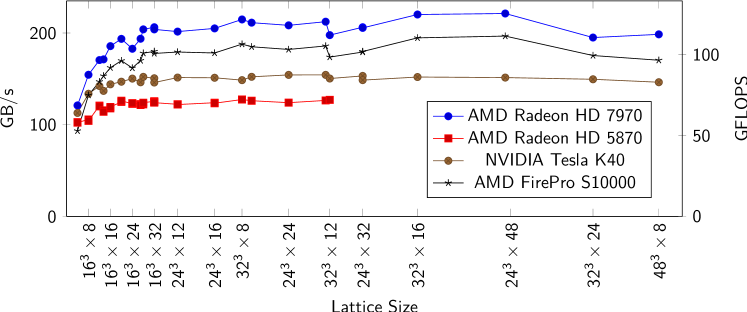
Figure 3: Performace of Wilson ${\not}D$ kernel for various lattice sizes on different devices in double precision.

The staggered $D_{KS}$ implementation, which plays the same role as ${\not}D$ regarding the overall speed of the code, shows also good performance on various lattice sizes (Figure 4). In this case we are able to utilize $\sim 70\%$ of the peak memory bandwidth on the AMD Radeon HD 5870 and AMD Radeon HD 7970. Due to its recent development, the implementation of the staggered code can be further optimized. So far no other benchmark for a possible comparison is present in the literature. Again, the code runs also on NVIDIA devices as shown in the figure. The performance is though also here lower for the same reasons explained above regarding the Wilson ${\not}D$.

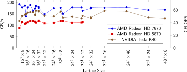
Figure 4: Performace of $D_{KS}$ kernel for various lattice sizes on different devices in double precision.

7 Algorithmic Performance

The full HMC application also performs very well compared to a reference CPU-based code tmLQCD [15] (see Figure 5). The tmLQCD performance was taken on one LOEWE -CSC node. Compared to tmLQCD, the older AMD Radeon HD 5870 is twice as fast. The newer AMD FirePro S10000 again doubles this performance. This essentially means that we gain a factor of 4 in speed, comparing a single GPU to a whole LOEWE -CSC node. In addition, it is interesting to look at the price-per-flop, which is much lower for the GPUs used then for the used CPUs.

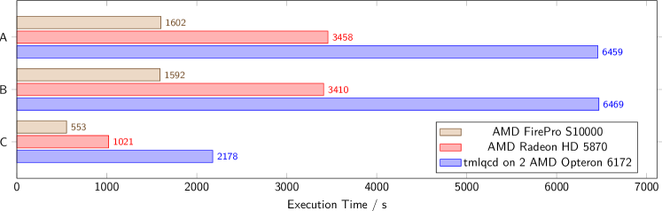
Figure 5: HMC performance for different Setups A, B and C (setup A having the smallest fermion mass) for $N_{\tau}=8,N_{\sigma}=24$. The HMC is compared on different GPUs and compared to a reference code [15] running on one LOEWE -CSC node.

As on-board memory is the biggest limiting factor on GPUs, using multiple GPUs is of great interest [16]. In CL²QCD it is possible to split the lattice in time direction [17].

8 Conclusions and Perspectives

We presented the OpenCL-based LQCD application CL²QCD. It has been successfully applied in finite temperature studies on LOEWE -CSC and SANAM supercomputers (see Table 2), providing a well-suited basis for future applications. CL²QCD is available at

In $N_{f}=2$ Lattice QCD studies we explore the phase diagram of QCD, in particular aiming at the chiral limit, where the order of the chiral transition is not resolved yet. Results obtained here can be used to constrain the physical phase diagram of QCD. The chiral limit is investigated in two independent approaches. On the one hand, in studies employing Twisted Mass Wilson fermions [18, 19, 20], we aim directly at the chiral limit at zero chemical potential. On the other hand, one can approach this issue by studying the phase structure of QCD at purely imaginary values of the chemical potential $\mu$, which we do with Wilson and staggered fermions [21, 22].

Additional features will be added to CL²QCD according to the needs of the physical studies. In the near future, these will cover the extension of Wilson fermions to $N_{f}=2+1$ flavours and the implementation of the clover discretization. Adding to that, optimizations of performances of staggered fermions and the inclusion of improved staggered actions are planned.

- [1] S. Duane et al. “Hybrid Monte Carlo” In Phys. Lett. B195, 1987, pp. 216–222 DOI: 10.1016/0370-2693(87)91197-X
- [2] Matthias Bach et al. “Optimized HPL for AMD GPU and multi-core CPU usage” In Comput. Sci. 26.3-4 Secaucus, NJ, USA: Springer-Verlag New York, Inc., 2011, pp. 153–164 DOI: 10.1007/s00450-011-0161-5
- [3] David Rohr et al. “An Energy-Efficient Multi-GPU Supercomputer” In Proceedings of the 16th IEEE International Conference on High Performance Computing and Communications, HPCC 2014, Paris, France. IEEE, 2014
- [4] O. Philipsen et al. “LatticeQCD using OpenCL” In PoS LATTICE2011, 2011, pp. 044 arXiv:1112.5280 [hep-lat]
- [5] Matthias Bach et al. “Lattice QCD based on OpenCL” In Comput.Phys.Commun. 184, 2013, pp. 2042–2052 DOI: 10.1016/j.cpc.2013.03.020
- [6] A. Shindler “Twisted mass lattice QCD” In Phys. Rept. 461, 2008, pp. 37–110 DOI: 10.1016/j.physrep.2008.03.001
- [7] R. Frezzotti and G.C. Rossi “Chirally improving Wilson fermions. 1. O(a) improvement” In JHEP 0408, 2004, pp. 007 DOI: 10.1088/1126-6708/2004/08/007
- [8] Martin Lüscher “A portable high-quality random number generator for lattice field theory simulations” In Computer Physics Communications 79.1, 1994, pp. 100 –110 DOI: 10.1016/0010-4655(94)90232-1
- [9] M. A. Clark and A. D. Kennedy “Accelerating staggered-fermion dynamics with the rational hybrid Monte Carlo algorithm” In Phys. Rev. D 75 American Physical Society, 2007, pp. 011502 DOI: 10.1103/PhysRevD.75.011502
- [10] M. Creutz “Monte Carlo Study of Quantized SU(2) Gauge Theory” In Phys. Rev. D21, 1980, pp. 2308–2315 DOI: 10.1103/PhysRevD.21.2308
- [11] Nicola Cabibbo and Enzo Marinari “A new method for updating SU(N) matrices in computer simulations of gauge theories” In Physics Letters B 119.4-6, 1982, pp. 387 –390 DOI: 10.1016/0370-2693(82)90696-7
- [12] A.D. Kennedy and B.J. Pendleton “Improved heatbath method for Monte Carlo calculations in lattice gauge theories” In Physics Letters B 156.5-6, 1985, pp. 393 –399 DOI: 10.1016/0370-2693(85)91632-6
- [13] Beck “Test Driven Development: By Example” Boston, MA, USA: Addison-Wesley Longman Publishing Co., Inc., 2002
- [14] Robert C. Martin “Clean Code: A Handbook of Agile Software Craftsmanship” Upper Saddle River, NJ, USA: Prentice Hall PTR, 2008
- [15] K. Jansen and C. Urbach “tmLQCD: a program suite to simulate Wilson Twisted mass Lattice QCD” In Comput. Phys. Commun. 180, 2009, pp. 2717–2738 DOI: 10.1016/j.cpc.2009.05.016
- [16] R. Babich “Scaling Lattice QCD beyond 100 GPUs”, 2011 arXiv:1109.2935 [hep-lat]
- [17] M. Bach et al. “Twisted-Mass Lattice QCD using OpenCL” In PoS LATTICE2013, 2014, pp. 032
- [18] O. Philipsen and L. Zeidlewicz “Cutoff effects of Wilson fermions on the QCD equation of state to ” In Phys. Rev. D81, 2010, pp. 077501 DOI: 10.1103/PhysRevD.81.077501
- [19] E.-M. Ilgenfritz et al. “Phase structure of thermal lattice QCD with twisted mass Wilson fermions” In Phys. Rev. D80, 2009, pp. 094502 DOI: 10.1103/PhysRevD.80.094502
- [20] F. Burger et al. “The thermal QCD transition with two flavours of twisted mass fermions”, 2011 arXiv:1102.4530 [hep-lat]
- [21] Owe Philipsen and Christopher Pinke “Nature of the Roberge-Weiss transition in QCD with Wilson fermions” In Phys. Rev. D 89 American Physical Society, 2014, pp. 094504 DOI: 10.1103/PhysRevD.89.094504
- [22] Claudio Bonati et al. “The chiral phase transition for two-flavour QCD at imaginary and zero chemical potential”, 2013 arXiv:1311.0473 [hep-lat]