Glueball masses in 2+1 dimensional SU(N) gauge theories with twisted boundary conditions

Abstract:

We analyze 2+1 dimensional Yang-Mills theory regularized on a lattice with twisted boundary conditions in the spatial directions. In previous work it was shown that the observables in the non-zero electric flux sectors obey the so-called $x$-scaling, i.e. depend only on the dimensionless variable $x\propto NL/b$ and the angle $\tilde{\theta}$ given by the parameters of the twist ($L$ being the length of the spatial torus and $b$ the inverse ’t Hooft coupling). It is conjectured that this scaling is obeyed by all physical quantities. In this work we extend the previous analyses to the zero electric flux (glueball) sector. We study the mass of the lightest scalar glueball in two theories with different $N$ but matching $x$ and $\tilde{\theta}$ in a wide range of couplings from the perturbative small-volume regime to the non-perturbative one. We find that the results are consistent with the $x$-scaling hypothesis.

1 Introduction

Large-$N$ gauge theories ($N$ being the degree of the gauge group) exhibit a number of peculiar features related to the fact that only the leading contribution in the so-called $N$-counting rules survives in the $N\to\infty$ limit (see e.g. Refs. [1, 2] for review). One particularly interesting feature of the large-$N$ limit is the emergence of the so-called large-$N$ equivalences, linking theories with different parameters such as the matter content, gauge groups or the spacetime volume on which the theories are defined [3, 5, 4].

In fact, one of the most renowned examples of such equivalences is the Eguchi-Kawai reduction [6], also known as volume reduction or volume independence, which (in the lattice language) relates two $SU(N)$ gauge theories: one defined on infinite lattice and the other defined on a toroidal lattice of arbitrarily small size (including one spacetime lattice site).

The Eguchi-Kawai reduction requires that the center symmetry in the small-volume theory remains unbroken, which turns out to be a non-trivial condition. One of the ways to fulfill it is to use twisted boundary conditions in the spacetime torus [7, 8, 9, 10]. Other methods include partial reduction (which requires keeping the physical volume of the reduced model large enough, $\gtrsim 1\textrm{fm}^{4}$) [11], the addition of adjoint fermions to the model [12, 13, 14] and the related idea of trace-deformed reduction [15].

Note that the large-$N$ equivalences are only strictly true in the $N\to\infty$ limit. In this work we follow a slightly different approach and analyze the interplay between finite $N$ and $L$, where $L$ denotes the size (in lattice units) of the spatial torus on which the theory is defined.

In our particular case, we analyze 2+1-dimensional lattice gauge theory (extensions to 3+1 dimensions are also possible, see Ref. [16]) defined on a spatial torus with twisted boundary conditions. The action of the model is given by:

$$S=Nb\sum_{n}\sum_{\mu\neq\nu}\left(N-z^{*}_{\mu\nu}(n)P_{\mu\nu}(n)\right),$$ (1)

where $n$ runs over the lattice of size $L\times L\times T$, $b$ is the inverse ’t Hooft coupling, $P_{\mu\nu}(n)$ is the plaquette and $z_{\mu\nu}$ is the twist tensor equal to 1 except at corner plaquettes in (1,2)-plane where it is equal to:

$$z_{ij}(n)=\exp\Big{(}i\epsilon_{ij}\frac{2\pi k}{N}\Big{)},$$ (2)

where $k$ is an integer known as the magnetic flux. We also define integer $\bar{k}$ as the modular multiplicative inverse of $k$:

$$k\bar{k}=1\ (\textrm{mod }N).$$ (3)

Our interest is motivated by the work of Ref. [17] where this setup was analyzed in the non-zero electric flux sector, which in the large volume corresponds to the $k$-string tensions. In this work it was shown, both in perturbation theory to all orders and in non-perturbative lattice calculations, that the $k$-string tensions depend only on the dimensionless scaling variable:

$$x=\frac{NL}{4\pi b}$$ (4)

and the angle determined by the coefficient $\bar{k}$:

$$\tilde{\theta}=\frac{2\pi\bar{k}}{N}.$$ (5)

Thus, for given twist, the physics of the non-zero flux sector depends on $N$ and $L$ only via the product $NL$. This can be thought as a generalized volume reduction where volume and gauge group size can be interchanged also at finite $N$.

The long-term goal of this work is to verify whether this fact holds also in the zero electric flux sector (corresponding to the glueball and torelon spectrum). In this paper we restrict ourselves to comparing the mass of the lightest scalar glueball in two theories:

1. $N=5$, $L=14$, $\bar{k}=2$, corresponding to $NL=70$, $\tilde{\theta}\approx 2.513$

2. $N=17$, $L=4$, $\bar{k}=7$, corresponding to $NL=68$. $\tilde{\theta}\approx 2.587$

The theories are chosen so that while the values of $N$ are vastly different, the values of the parameters $x$ and $\tilde{\theta}$, determining the physical behaviour (at least in the non-zero electric flux sector), are close within a couple percent. Thus, if the hypothesis that this behaviour extends to the glueball sector is true, the values of the glueball mass should be approximately equal in the two theories for all values of the coupling $b$ (corresponding to different values of the scaling parameter $x$).

2 Calculation

The calculation of the glueball masses is performed in a wide range of couplings. In particular we need to deal with several regions in which the behaviour is widely different – knowledge from earlier works [17, 18] as well as some hindsight allow us to distinguish three such regions:

1. Perturbative, small-volume region: $x\lesssim 0.5$.

2. Intermediate region: $0.5\lesssim x\lesssim 3$.

3. Large-volume region: $x\gtrsim 3$. Note: to have better access to the large-volume region we also use the theories with the lattice torus size $L$ doubled.

The extraction of the ground state for the glueballs is not an easy task and requires variational analysis, using the solution of the Generalized Eigenvalue Problem (called GEVP in the following).

The observables $O_{i}(t)$ we use are rectangular Wilson loops and squared moduli of multi-winding spatial Polyakov loops $|\textrm{Tr}\,P^{\,n}|^{2}$, projected to zero momentum and angular momentum.

We employ three different levels of APE [19] smearing on the loops (7, 14 and 21 steps, with smearing parameter $\alpha=0.475$) and, instead of blocking, use Wilson loops of large sizes, trying, for given values of the coupling, to choose the loop sizes whose correlators give good signal at large time separations (i.e. trying to follow the physical size of the glueball). That includes, in particular using Wilson loops larger than the spatial extent of the lattice for small $x$.

From the observables we construct the correlation matrix:

$$C_{ij}(t)=\sum_{t^{\prime}}\langle O_{i}(t^{\prime}+t)O_{j}(t^{\prime})\rangle-\langle O_{i}(t^{\prime}+t)\rangle\langle O_{j}(t^{\prime})\rangle,$$ (6)

on which we solve the GEVP for $t_{0}=a$, $t_{1}=t_{0}+a$ (we find that in practice, increasing the value of $t_{0}$ does not change the results significantly):

$$C(t_{1})v=C(t_{0})\lambda v.$$ (7)

We then use the obtained eigenvectors $v$ to change the basis of $C(t)\to\tilde{C}(t)$ for all values of $t$ and use the diagonal values of $\tilde{C}(t)$ to extract the plateau ranges and subsequently perform fits on the selected ranges.

One subtlety when fitting outside the large-volume region is that the finite-temperature corrections turn out to play a sizeable role in the correlators for the temporal extents $T$ of the lattices used ($T=72$, except the large-volume region, where $T=36$). In perturbation theory one can show that the correction is proportional to $\exp(-mT/2)$ where $m$ is the mass of the lightest glueball, rather than $\exp(-mT)$; the factor 2 comes from the fact that there is a single gluon propagating around the temporal torus which has energy $m/2$. This forces us to include the effect of the constant term on the fits. We do that using the midpoint-subtracted correlators [20] in the effective mass plots and the fits.

The correlation matrix typically consists of approximately $15$ operators. We verify whether the basis allows for reliable GEVP solution by first solving it on non-symmetrized correlation matrix – the breakdown of the non-symmetrized GEVP signals insufficient signal-to-noise ratio. The GEVP and basis change are done in quadruple (128 bit) floating-point precision to avoid adding round-off errors to the problem.

3 Results

The physics of the problem is significantly different in the three regions of interest. In the large-volume (large-$x$) region the result is expected to be close to the non-twisted large-volume calculations. In this region the operators with largest overlap to the ground state are the contractible Wilson loops. The choice of boundary conditions should be irrelevant in large volume thus we expect that the results are consistent with [18].

On the other hand, in the small-$x$ region, the expectations can be made using perturbation theory. In the twisted theory, the leading contribution for the lowest energy is [17]:

$${b\cal{E}}={1\over x}-2G(\tilde{\theta}/2\pi)-{3\over 4\pi^{2}}\sin^{2}(\tilde{\theta}/2)\,,$$ (8)

where we have introduced the function:

$$G(z)=-{1\over 16\pi^{2}}\int_{0}^{\infty}{dt\over\sqrt{t}}\,\Big{(}\theta_{3}(0,it)\big{(}\theta_{3}(0,it)-\theta_{3}(z,it)\big{)}-{1\over t}\Big{)}.$$ (9)

with $\theta_{3}$ the Jacobi Theta function. Also, the operator with the highest overlap to the ground state is $|\textrm{Tr}\,P^{\,\bar{k}}|^{2}$, corresponding to the pair of (mutually conjugate, i.e. carrying momenta with opposite signs) gluonic operators, each having the lowest possible momentum given by

$$|\vec{p}|=\frac{2\pi}{NL}\,.$$ (10)

The hardest to analyze is the intermediate-$x$ region where there are no theoretical expectations and where different states contribute to the result. We expect level crossing in this region and many states with similar energies may be found. We find that in this region it is necessary to include $|\textrm{Tr}\,P^{\,\bar{k}}|^{2}$, $|\textrm{Tr}\,P|^{2}$ and the Wilson loops whose contribution to the ground state changes as $x$ goes from the perturbative to the large-volume regime.

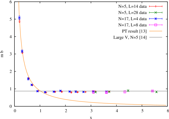
(a)

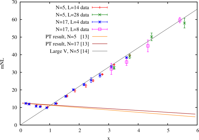
(b)

Figure 1: The results for the lightest scalar glueball mass as a function of the $x$ variable. Two quantities are shown: Fig. (a) shows the lattice results rescaled times the inverse ’t Hooft coupling and in Fig. (b) the lattice results are rescaled by a factor $NL$. The error bars are purely statistical, coming from the jackknife estimation of errors from the correlated fits. In Fig. (a) only one perturbative result is drawn as the results for the two theories are indistinguishable.

The results, together with theoretical expectations, are presented in Fig. 1. Fig. 1a presents the results in the units of $mb=m/(g^{2}N)$ ($g^{2}$ has dimension of mass in 2+1 dimensions). On Fig. 1b the same results are presented in different units, introduced as following. The standard rescaling in finite volume analyses is done using the control variable $z=mL$ [21]. On the other hand, if the $x$-scaling hypothesis is correct, we expect the data points to be governed rather by the combination $mNL$, which is presented in Fig. 1b.

The plots show a rather striking agreement between the two theories. The results for $N=5$ and $N=17$ are consistent within errors for all values of $x$ analyzed. This is a strong confirmation of the $x$-scaling hypothesis also in the zero electric flux sector.

Another observation is that the change of behaviour between the perturbative and large-volume like behaviour is rather abrupt. Even in the region $1\lesssim x\lesssim 3$ where the inclusion of the moduli of Polyakov loops in the GEVP basis is necessary to get satisfying plateaux, the results follow the large-volume value closely.

4 Conclusions & outlook

We verified that the mass of the lightest scalar glueball in 2+1 dimensions with twisted spatial boundary conditions is consistent between theories with $N=5$ and $N=17$ with matching values of the parameters $x\propto NL/b$ and $\tilde{\theta}\propto\bar{k}/N$ for a very wide range of couplings, including all regions of physical interest.

The equality of masses of the glueball states, belonging to the zero electric flux sector, gives a strong support to the $x$-scaling hypothesis, which states that the physics of twisted theories in 2+1 dimensions can be accurately described by using solely two dimensionless parameters $x$ and $\tilde{\theta}$, as was already verified in the non-zero electric flux sector (corresponding to the $k$-string tensions) in Ref. [17].

The analysis presented here can be improved in many ways. To reduce the systematic errors the introduction of well-defined criteria for the choice of plateau ranges is necessary. Choosing the plateaux “by the eye” is particularly problematic in the presence of the midpoint subtraction procedure. We plan to eliminate this difficulty by choosing the temporal extent $T$ to be large enough to suppress the finite-temperature related constant term. This will also allow to use the GEVP in the way done by ALPHA Collaboration which puts the contamination by excited states under better control [22].

For the forthcoming publication we also plan to include another value of $N$ and study the $\bar{k}$ dependence, as well as calculate the mass of the tensor glueball.

References

- [1] A. V. Manohar, arXiv:hep-ph/9802419.
- [2] B. Lucini and M. Panero, Phys. Rept. 526, 93 (2013) [arXiv:1210.4997 [hep-th]].
- [3] C. Lovelace, Nucl. Phys. B201, 333 (1982).
- [4] A. Armoni, M. Shifman and G. Veneziano, Nucl. Phys. B667, 170 (2003) [arXiv:hep-th/0302163].
- [5] P. Kovtun, M. Ünsal and L. G. Yaffe, JHEP 0507, 008 (2005) [arXiv:hep-th/0411177].
- [6] T. Eguchi and H. Kawai, Phys. Rev. Lett. 48, 1063 (1982).
- [7] A. González-Arroyo and M. Okawa, Phys. Lett. B120, 174 (1983).
- [8] A. González-Arroyo and M. Okawa, Phys. Rev. D27, 2397 (1983).
- [9] A. González-Arroyo and M. Okawa, JHEP 1007, 043 (2010) [arXiv:1005.1981 [hep-lat]].
- [10] A. González-Arroyo and M. Okawa, Phys. Lett. B718, 1524 (2013) [arXiv:1206.0049 [hep-lat]].
- [11] J. Kiskis, R. Narayanan and H. Neuberger, Phys. Lett. B574, 65 (2003) [arXiv:hep-lat/0308033].
- [12] P. Kovtun, M. Ünsal, L. G. Yaffe, JHEP 0706, 019 (2007) [hep-th/0702021].
- [13] G. Başar, A. Cherman, D. Dorigoni and M. Ünsal, Phys. Rev. Lett. 111, 121601 (2013) [arXiv:1306.2960 [hep-th]].
- [14] M. Koreń, PhD thesis, Kraków, 2013, arXiv:1312.5351 [hep-lat].
- [15] M. Ünsal, L. G. Yaffe, Phys. Rev. D78, 065035 (2008) [0803.0344 [hep-th]].
- [16] M. García Pérez, A. González-Arroyo and M. Okawa, Int. J. Mod. Phys. A29, 1445001 (2014) [arXiv:1406.5655 [hep-th]].
- [17] M. García Pérez, A. González-Arroyo and M. Okawa, JHEP 1309, 003 (2013) [arXiv:1307.5254 [hep-lat]].
- [18] M. Teper, Phys. Rev. D59, 014512 (1999) [arXiv:hep-lat/9804008].
- [19] M. Albanese et al. [APE Collaboration], Phys. Lett. B192, 163 (1987).
- [20] T. Umeda, Phys. Rev. D75, 094502 (2007) [arXiv:hep-lat/0701005].
- [21] M. Lüscher and G. Münster, Nucl. Phys. B232, 445 (1984).
- [22] B. Blossier, M. DellaMorte, G. von Hippel, T. Mendes, and R. Sommer, JHEP 0904, 094 (2009) [arXiv:0902.1265 [hep-lat]].