A new algorithm for wavelet-based heart rate variability analysis

Abstract

One of the most promising non-invasive markers of the activity of the autonomic nervous system is Heart Rate Variability (HRV). HRV analysis toolkits often provide spectral analysis techniques using the Fourier transform, which assumes that the heart rate series is stationary. To overcome this issue, the Short Time Fourier Transform is often used (STFT). However, the wavelet transform is thought to be a more suitable tool for analyzing non-stationary signals than the STFT. Given the lack of support for wavelet-based analysis in HRV toolkits, such analysis must be implemented by the researcher. This has made this technique underutilized.

This paper presents a new algorithm to perform HRV power spectrum analysis based on the Maximal Overlap Discrete Wavelet Packet Transform (MODWPT). The algorithm calculates the power in any spectral band with a given tolerance for the band’s boundaries. The MODWPT decomposition tree is pruned to avoid calculating unnecessary wavelet coefficients, thereby optimizing execution time. The center of energy shift correction is applied to achieve optimum alignment of the wavelet coefficients. This algorithm has been implemented in RHRV, an open-source package for HRV analysis. To the best of our knowledge, RHRV is the first HRV toolkit with support for wavelet-based spectral analysis.

1 Introduction

Heart Rate Variability (HRV) refers to the variation over time of the intervals between consecutive heartbeats. Since the heart rhythm is modulated by the autonomic nervous system (ANS), HRV is thought to reflect the activity of the sympathetic and parasympathetic branches of the ANS. The continuous modulation of the ANS results in continuous variations in heart rate. One of the most powerful HRV analysis techniques is based on the spectral analysis of the time series obtained from the distances between each pair of consecutive heartbeats. The HRV power spectrum is a useful tool as a predictor of multiple pathologies [1], [2].

Akselrod et al. [3] described three components in the HRV power spectrum with physiological relevance: the very low frequency (VLF) component (frequencies below 0.03 Hz), which is modulated by the renin-angiotensin system; the low frequency (LF) component (0.03-0.15 Hz), which is thought to be of both sympathetic and parasympathetic nature; and the high frequency (HF) component (0.18-0.4 Hz), which is related to the parasympathetic system. At present, there is no absolute consensus on the precise limits of the boundaries of these three bands. In the literature we can find authors who use slightly different bands’ boundaries [4].

There exist several HRV spectral analysis techniques. These techniques may be classified as nonparametric and parametric [5]. The main advantage of the nonparametric methods is the simplicity and speed of the algorithm used (The Fast Fourier Transform). The main advantage of the parametric methods is that they give smoother spectral components. However, parametric methods present problems regarding to correct model order selection. Although these techniques are widely used, they have no temporal resolution. This severely limits their ability to analyze non-stationary signals and transient phenomena. To alleviate this limitation temporal windows are often used, so that small segments of the whole signal are analyzed. Among these techniques we may highlight the Short Time Fourier Transform (STFT) [6]. However, time-frequency resolution of the STFT depends on the spread of the window used. Thus, the STFT has fixed time-frequency resolution: high frequency resolution implies poor time resolution and vice versa. Conversely to Fourier, the wavelet transform performs time-frequency analysis and it is recognized as a powerful tool to study non-stationary signals [7].

HRV analysis toolkits such as Kubios HRV [8] or aHRV [9] only enable HRV spectral analysis based on the Fourier transform or parametric methods. To the best of our knowledge, the only option for using the wavelet transform in HRV analysis is to manually implement the algorithms, probably with the support of some general wavelet library. This is tedious, and prone to error. Although some researchers have done this [10], [11], many more (especially those with a medical background) choose to use Fourier-based tools, even when they know that the signal being analyzed is non-stationary. A query in the PubMed database with the terms “heart rate variability Fourier transform” returns 660 articles, while a query with the terms “heart rate variability wavelet transform” only returns 145 articles. The lack of tools for carrying out HRV analysis using the wavelet transform has made this potentially superior analysis technique underutilized in comparison with the Fourier transform.

In this paper we present an algorithm to perform HRV power spectrum analysis based on the Maximal Overlap Discrete Wavelet Packet Transform (MODWPT). The algorithm calculates the spectrogram in any frequency band, allowing a certain tolerance for the position of the band’s boundaries. The algorithm has been validated over simulated and real RR series. Its capability for identifying fast changes in the RR series’ spectral components has been compared with the STFT and a windowed version of the Burg method, showing that these techniques miss some transient changes that are successfully identified by the wavelet transform. We have implemented the algorithm in RHRV, an open-source package for HRV analysis publicly available on the Internet. A previous version of this algorithm was published in [12].

Section 2 starts with a brief review of the wavelet transform, with particular attention to the MODWPT, and then introduces our algorithm to perform HRV power spectrum analysis. Section 2.5 provides a short description of the implementation of the algorithm in the RHRV package. Section 3 presents a comparison between our algorithm, the STFT and the windowed Burg method over simulated and real RR series. Finally, the results of this paper are discussed and some conclusions are given.

2 Material and methods

A brief review of some important wavelet concepts for our algorithm is now given. A wavelet is a small wave $\psi(t)$ (oscillating function) that is well concentrated in time. This function must have unitary norm $\|\psi\|=1$ and verify the so-called admissibility condition: $\int_{-\infty}^{\infty}\psi(t)dt=0.$ $\psi(t)$ can be translated and dilated in time, yielding a set of wavelet functions:

$$\psi_{u,s}(t)=\frac{1}{\sqrt{s}}\psi\left(\frac{t-u}{s}\right),$$ (1)

where $s>0$ is a dilation factor, and $u$ is a real number representing the translations. As $\psi$ generates all $\psi_{u,s}$ functions, it is called mother wavelet.

A continuous wavelet transform measures the time-frequency variations of a signal $f$ by correlating it with $\psi_{u,s}$

$$Wf(u,s)=\int_{-\infty}^{\infty}f(t)\psi^{*}_{u,s}(t)dt.$$ (2)

In order to make the wavelet transform implementable on a computer, both dilation and translation factors must be discretized. This can be achieved as follows:

$$\left\{\psi_{j,n}=\frac{1}{\sqrt{2^{j}}}\psi\left(\frac{t-2^{j}n}{2^{j}}\right)\right\}_{j,n\;\in\;\mathbb{Z}.}$$ (3)

This family is an orthonormal basis of $\mathbf{L^{2}(\mathbb{R})}$. Orthogonal wavelets dilated by $2^{j}$ can be used to study signal variations at the resolution $2^{-j}$. Thus, these families of wavelets originate a multiresolution signal analysis. Multiresolution analysis projects signals at various resolution spaces $\mathbf{V}_{j}$. Each $\mathbf{V}_{j}$ space contains all possible approximations at the resolution $2^{-j}$. Thus, each decomposition level increases the spectral resolution of the decomposition, at the expense of losing temporal resolution. Let $\{\mathbf{V}_{j}\}_{j\in\mathbb{Z}}$ be a multiresolution approximation verifying $\mathbf{V}_{j+1}\subset\mathbf{V}_{j}\;\forall j\in\mathbb{Z}$ and let $\mathbf{W}_{j}$ be the orthogonal complement of $\mathbf{V}_{j}$ in $\mathbf{V}_{j-1}$: $\mathbf{V}_{j-1}=\mathbf{V}_{j}\oplus\mathbf{W}_{j}$. According to [13], the families

$$\left\{\phi_{j,n}=\frac{1}{\sqrt{2^{j}}}\phi\left(\frac{t-2^{j}n}{2^{j}}\right)\right\}_{n\in\mathbb{Z}}\qquad\text{ and }\qquad\left\{\psi_{j,n}=\frac{1}{\sqrt{2^{j}}}\psi\left(\frac{t-2^{j}n}{2^{j}}\right)\right\}_{n\in\mathbb{Z}}$$ (4)

are an orthonormal basis for $\mathbf{V}_{j}$ and $\mathbf{W}_{j}$, respectively, for all $j\in\mathbb{Z}$. $\psi_{j,n}$ are the wavelet functions and $\phi_{j,n}$ are the scaling functions.

Thus, we can approximate any function $f$ $\epsilon\;\mathbf{L^{2}(\mathbb{R})}$ at resolution $2^{-j}$ as

$$P_{\mathbf{V}_{j}}f=\sum_{n=-\infty}^{\infty}\langle f,\phi_{j,n}\rangle\phi_{j,n}=\sum_{n=-\infty}^{\infty}a_{j}[n]\phi_{j,n}$$ (5)

and the orthogonal projection of $f$ onto detail space $\mathbf{W}_{j}$ is:

$$P_{\mathbf{W}_{j}}f=\sum_{n=-\infty}^{\infty}\langle f,\psi_{j,n}\rangle\psi_{j,n}=\sum_{n=-\infty}^{\infty}d_{j}[n]\psi_{j,n}.$$ (6)

where $a_{j}[n]$ and $d_{j}[n]$ are called the approximation and detail coefficients, respectively.

Mallat proved [7] that both approximation and detail coefficients may be calculated using a filter bank. Let $h[n]$ and $g[n]$ be the FIR filters that will be used to compute the approximation and detail coefficients, respectively. It has been proven [13] that the filter $h[n]=\langle\frac{1}{\sqrt{2}}\phi\left(\frac{t}{2}\right),\phi\left(t-n\right)\rangle$ and that $g[n]=\langle\frac{1}{\sqrt{2}}\psi\left(\frac{t}{2}\right),\phi\left(t-n\right)\rangle$. $g[n]$ and $h[n]$ can be regarded as an approximation to a high-pass filter (the wavelet filter) and to a low-pass filter (the scaling filter), respectively. By applying recursively over the approximation coefficients the same filtering operation followed by sub-sampling by two, we obtain the multiresolution expression of $f$. This algorithm, known as the pyramid algorithm, is the most efficient way of computing the Fast Orthogonal Wavelet Transform (FOWT) [13].

2.1 MODWPT

Given that the filtering operation is only applied over the approximation coefficients, the FOWT only provides information on a limited set of frequency bands which need not be the ones used in the HRV analysis. A more suitable wavelet transform is needed for our algorithm: the wavelet packet decomposition (WPD). Instead of dividing only the approximation coefficients $a_{j}[n]$, both detail and approximation coefficients are decomposed successively by applying high pass and low pass filters to each set of coefficients.

Among the WPD transforms we have chosen the MODWPT [14] because it is less sensitive to the starting point of the time series and it is applicable to non dyadic sequences. Furthermore, the MODWPT avoids the sub-sampling step, and therefore it has the same number of wavelet coefficients in every decomposition level. This simplifies computations involving different decomposition levels.

The $j^{th}$ level of the MODWPT decomposes the frequency interval $[0,f_{s}/2]$, where $f_{s}$ is the sampling frequency of the original signal $f$, into $2^{j}$ equal width intervals (see Fig. 1). Thus, the $n^{th}$ node (beginning at zero) in the $j^{th}$ level of the decomposition tree, the $(j,n)$ node, is associated with the frequency interval $\frac{f_{s}}{2^{j+1}}\left[n,n+1\right]$. Each node will have $N$ wavelet coefficients associated, $N$ being the length of the sampled signal $f$. The $N$-dimensional vector $\mathbf{W}_{j,n}$ will denote the $N$ wavelet coefficients associated with the $(j,n)$ node.

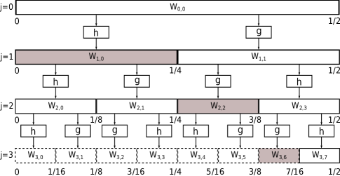
Figure 1: MODWPT decomposition tree with the nodes selected to cover the band $[0,7/16]$ Hz. $\mathbf{W}_{0,0}$ represents the original signal, $f(t).$

MODWPT coefficients fulfill that:

$$\|f\|^{2}=\sum_{n=0}^{2^{j}-1}\|\mathbf{W}_{j,n}\|^{2}\quad\forall j.$$ (7)

Therefore, given a frequency band $\left[f_{1},f_{2}\right]=\frac{f_{s}}{2^{j+1}}\left[k,k^{\prime}+1\right]$, $f_{s}$ being the sampling frequency and $k$, $k^{\prime}$ and $j$ integers, the spectral power in $\left[f_{1},f_{2}\right]$, $P(\left[f_{1},f_{2}\right])$, can be calculated from the appropriate MODWPT coefficients. We just need to find the nodes $(j,k)$ and $(j,k^{\prime})$ and compute the spectral power in the band $\left[f_{1},f_{2}\right]$ as:

$$P(\left[f_{1},f_{2}\right])=\sum_{n=k}^{k^{\prime}}\|\mathbf{W}_{j,n}\|^{2}.$$ (8)

2.2 Finding a proper cover for a set of frequency bands

Equation (8) can only be applied to bands that can be written as $\frac{f_{s}}{2^{j+1}}\left[k,k^{\prime}+1\right]$, $f_{s}$ being the sampling frequency and $k$, $k^{\prime}$ and $j$ integers. In an HRV spectral analysis the user can be interested in bands that cannot be written this way. This forces us to permit a certain error when we try to cover the bands with coefficients obtained from the MODWPT decomposition. Let $[f_{l},f_{u}]$ be the band, and let $\epsilon_{l}$ and $\epsilon_{u}$ be the maximum errors allowed for the beginning and the ending of the band, respectively. We need to find a node $(j,n)$ whose lower frequency corresponds roughly to $f_{l}$ with the tolerance allowed by $\epsilon_{l}$, i.e.:

$$\left|f_{l}-\frac{f_{s}}{2^{j+1}}n\right|\leq\epsilon_{l}.$$ (9)

Analogously, we also need to find a node $(j^{\prime},n^{\prime})$ whose upper frequency corresponds roughly to $f_{u}$ with the tolerance allowed by $\epsilon_{u}$:

$$\left|f_{u}-\frac{f_{s}}{2^{j^{\prime}+1}}(n^{\prime}+1)\right|\leq\epsilon_{u}.$$ (10)

We shall refer to (9) and (10) as the cover conditions.

The level $j$ of the decomposition tree in which the node $(j,n)$ that fulfills (9) is found needs not be the same as the level $j^{\prime}$ in which the node $(j^{\prime},n^{\prime})$ that fulfills (10) is found. But, (8) requires that $j=j^{\prime}$. To avoid this problem we may think that, after the nodes $(j,n)$ and $(j^{\prime},n^{\prime})$ have been found, we could descend the node that is at the higher level, decomposing it to the level of the other node [12]. However, when descending to low levels in the frequency decomposition tree, frequency resolution increases and temporal resolution decreases because of the Gabor-Heisenberg uncertainty principle for signals: $\Delta t\Delta f\geq 1/2$ [15]. Furthermore, wavelet coefficients suffer a circular time shift as a result of the use of wavelet filters. As we descend to lower levels, the circular shift will be more pronounced as we perform more convolutions. Therefore, to obtain a good temporal resolution, we should avoid descending to deep levels of the tree.

Let’s suppose that, when looking for a cover for the band of interest $\left[f_{1},f_{2}\right]$, the nodes $(j,n)$ and $(j^{\prime},n^{\prime})$ are selected. These nodes must fulfill the cover conditions (9) and (10) with $f_{l}=f_{1}$ and $f_{u}=f_{2}$. Generally, the nodes $(j,n)$ and $(j^{\prime},n^{\prime})$ are at different levels (i.e., $j\neq j^{\prime}$). Furthermore, these nodes cover the band $\frac{f_{s}}{2^{j+1}}\left[n,n+1\right]\cup\frac{f_{s}}{2^{j^{\prime}+1}}\left[n^{\prime},n^{\prime}+1\right]$, but the band $f_{s}\left[\frac{n+1}{2^{j+1}},\frac{n^{\prime}}{2^{j^{\prime}+1}}\right]=\left[f^{\prime}_{1},f^{\prime}_{2}\right]$ remains uncovered (see nodes $(1,0)$ and $(3,6)$ of Fig. 1). The problem has been reduced to finding a cover for the band $\left[f^{\prime}_{1},f^{\prime}_{2}\right]$. Thus, new nodes will be selected fulfilling the cover conditions (9) and (10), with $f_{l}=f^{\prime}_{1}$ and $f_{u}=f^{\prime}_{2}$. The complete cover of $\left[f_{1},f_{2}\right]$ can be achieved applying this technique recursively. The set of nodes resulting from this cover will be referred to as $\Gamma$.

There may be overlap between the bands associated with the nodes $(j,n)$ and $(j^{\prime},n^{\prime})$ (the original nodes fulfilling the cover conditions). This overlap will occur if a node is the parent of the other node or if both nodes are equal. If $(j,n)=(j^{\prime},n^{\prime})$, the node covers all the band and the search has ended. If the node $(j^{\prime},n^{\prime})$ is a child of the node $(j,n)$, we shall replace the node $(j,n)$ with its (unique) child verifying (9): the node $(j+1,2n)$. Thus, the algorithm continues with the nodes $(j+1,2n)$ and $(j^{\prime},n^{\prime})$. The process shall be repeated until there is no overlap between the two nodes fulfilling the cover condition. Similarly, if the node $(j,n)$ is a child of the node $(j^{\prime},n^{\prime})$, we replace the node $(j^{\prime},n^{\prime})$ with the node $(j^{\prime}+1,2n^{\prime}+1)$.

Figure 1 illustrates the cover process for the band $\left[0,7/16\right]$ Hz with $f_{s}=1$ Hz and $\epsilon_{u}=\epsilon_{l}=0.01$ using the “nodes at the same level” criteria used in [12] (dashed nodes) and the “nodes at different levels” criteria proposed here (dark nodes).

There exist multiple covers of any band $\left[f_{l},f_{u}\right]$. Our algorithm builds a cover using the nodes of the higher levels of the MODWPT tree. This selection criteria leads to a cover that minimizes temporal shift and maximizes temporal resolution. Furthermore, this cover also minimizes the number of nodes.

Equation (8) cannot be applied to this decomposition, because the decomposition uses nodes from different levels. However, because of the wavelet coefficients property

$$\|\mathbf{W}_{j,n}\|^{2}=\|\mathbf{W}_{j+1,2n}\|^{2}+\|\mathbf{W}_{j+1,2n+1}\|^{2},$$ (11)

we may write (8) as

$$P(\left[f_{1},f_{2}\right])\approx\sum_{n=k}^{k^{\prime}}\|\mathbf{W}_{j,n}\|^{2}=\sum_{\mathbf{W}_{j,n}\;\epsilon\;\Gamma}\|\mathbf{W}_{j,n}\|^{2}.$$ (12)

In practical applications, the complete MODWPT decomposition tree will be rarely needed. In order to improve the execution time of wavelet analysis we have developed a pruning algorithm that we call Pruned MODWPT (PMODWPT). The PMODWPT, instead of expanding every node of the decomposition tree will only calculate those children required to cover a frequency band. Figure 2 illustrates the pruning performed when calculating the power of the band $\left[0,3/8\right]$ Hz being $f_{s}=2$ Hz.

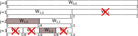
Figure 2: Prune procedure using the PMODWPT. The crosses indicates which nodes have been pruned.

2.3 Shift correction

As a consequence of the frequency-dependent phase response of the wavelet filters, it is necessary to keep track of which wavelet coefficients contain the energy contribution of a given portion of the signal being analyzed (see Fig. 3). That is, the wavelet coefficients must be corrected so that they can be accurately aligned with the original time series.

Hess-Nielsen and Wickerhauser proposed in [16] a technique to compute shift corrections exact for linear phase filters, and showed how to estimate the perturbation that a deviation from linear phase produces. This suggests that the method will produce better results with filters whose phase does not deviate much from a linear phase filter. Thus, this algorithm can be used to compute approximate shift corrections for a wide range of wavelets, including least asymmetric and extremal phase Daubechies, Symmlet or Coiflet wavelets.

Time shifts proposed in [16] are based on the notion of the “center of energy” of a filter. Let $a_{l}$ be a filter of length $l$. Its center of energy, $E\left\{a_{l}\right\}$ , is given by:

$$E\left\{a_{l}\right\}=\frac{\underset{n=0}{\overset{l-1}{\sum}}n\cdot a_{l}[n]^{2}}{\underset{n=0}{\overset{l-1}{\sum}}a_{l}[n]^{2}}$$ (13)

The time shift needed for the node $(j,n)$ of the MODWPT is always an advance (shift to the left) of $|p_{j,n}|$ units that is given by [16]

$$|p_{j,n}|=C_{j,n}(E\left\{g\right\}-E\left\{h\right\})+(2^{j}-1)E\left\{h\right\},$$ (14)

where $C_{j,n}$ is the bit-reversal of the binary gray code which encodes each of the MODWPT tree nodes [16].

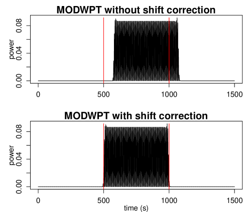
Figure 3: Time shift using MODWPT without (top) and with (bottom) “Center of Energy” correction. The vertical lines indicate where spectral power should be.

2.4 Wavelet-based HRV analysis

Listing 1 shows the pseudocode of our wavelet-based HRV analysis algorithm. The function waveletAnalysis takes as input parameters the interpolated and filtered RR series, the boundaries of the frequency bands, the wavelet to be used in the analysis, the sampling frequency of the RR series and the tolerance allowed when covering the frequency bands to be analyzed. The algorithm starts by finding the covers for each of the bands in which the user wants to calculate the spectral power. The calculateCover function implements the recursive covering algorithm presented in section 2.2. The getNode function selects the initial nodes fulfilling the cover conditions given by (9) and (10). It expands the node whose frequency interval contains the boundary frequency ($f$). If none of its children verify the cover condition for $f$, the child containing $f$ is selected and the process is repeated. The fillGapsBetweenNodes function completes the cover given a pair of initial nodes: $(j,n)$ and $(k,m)$ that fulfill (9) and (10), respectively. This function distinguishes the four cases discussed in section 2.2: $(j,n)=(k,m)$; $(k,m)$ is a child of the $(j,n)$ node; $(j,n)$ is a child of $(k,m)$ or the general case where there is an uncovered band.

Once the cover for the bands has been found, the wavelet coefficients are computed using the PMODWPT. Note that we use a single decomposition tree to calculate the power in all the bands. The shift correction described in section 2.3 is computed using shiftCorrection. The target nodes are specified to avoid applying corrections to nodes that will not be used in subsequent calculations. Since the wavelet and scaling filters are involved in (14), the wavelet used to perform the analysis must also be specified in the shiftCorrection function. Finally, the spectrogram of each band is computed with $\sum_{\mathbf{W}_{j,n}\;\epsilon\;\Gamma}|\mathbf{W}_{j,n}|^{2}$ by the getSpectrogram function.

Listing 1: Pseudocode of our wavelet-based HRV analysis algorithm.

⬇

waveletAnalysis($rr$, $VLFmin$, $VLFmax$, $LFmin$, $LFmax$, $HFmin$, $HFmax$,$wavelet$, $f_{s}$,$bandtolerance$){

$VLFnodes$=calculateCover($[VLFmin,VLFmax]$,$f_{s}$,$bandtolerance$)

$LFnodes$=calculateCover($[LFmin,LFmax]$,$f_{s}$,$bandtolerance$)

$HFnodes$=calculateCover($[HFmin,HFmax]$,$f_{s}$,$bandtolerance$)

$wrr$=PMODWPT($rr$,$wavelet$,$VLFnodes\cup LFnodes\cup HFnodes$)

$wrr$ = shiftCorrection($wrr$,$wavelet$,$VLFnodes\cup LFnodes\cup HFnodes$)

$VLFpower$=getSpectrogram($wrr$,$VLFnodes$)

$LFpower$=getSpectrogram($wrr$,$LFnodes$)

$HFpower$=getSpectrogram($wrr$,$HFnodes$)

return($VLFpower$,$LFpower$,$HFpower$)

}

calculateCover([$f_{l}$,$f_{u}$],$f_{s}$,$error$){

if ($f_{u}$==$f_{l}$ ) return($\left\{\right\}$)

$W_{j,n}$=getNode($f_{l}$,$f_{s}$,$error$)

$W_{k,m}$=getNode($f_{u}$,$f_{s}$,$error$)

return(fillGapsBetweenNodes($W_{j,n}$,$W_{k,m}$,$f_{s}$,$error$))

}

getNode($f$,$f_{s}$,$error$,$type$){

$i$=$1$

$nodeToExpand=0$

while($TRUE$){

$b_{j}$=$nodeToExpand$

$\Delta$ = $\frac{f_{s}}{2^{i+1}}$

for ($j$ in $(2\cdot b_{j}):(2\cdot b_{j}+1)$){

$interval$= $[j\Delta,(j+1)\Delta]$

if ($f$ $\in$ $interval$) $nodeToExpand$=$j$

if ($interval$ verifies band cover condition for $f$ and $error$) return ($W_{i,j}$)

}

$i=i+1$

}

}

fillGapsBetweenNodes($W_{j,n}$,$W_{k,m}$,$f_{s}$,$error$){

if($W_{j,n}$==$W_{k,m}$) return($W_{j,n}$)

if($W_{k,m}$ is Child of $W_{j,n}$) return(fillGapsBetweenNodes($W_{j+1,2n}$,$W_{k,m}$,$f_{s}$,$error$))

if($W_{j,n}$ is Child of $W_{k,m}$) return(fillGapsBetweenNodes($W_{j,n}$,$W_{k+1,2m+1}$,$f_{s}$,$error$))

$mediumNodes$=calculateCover($f_{s}\left[\frac{n+1}{2^{j+1}},\frac{m}{2^{k+1}}\right]$,$f_{s}$,$error$)

return($\left\{W_{j,n},W_{k,m}\right\}\cup\;mediumNodes$)

}

getSpectrogram($wrr$,$nodes$){

$S_{\left\{\mathbf{x}\right\}}[m]=0$

for ($W_{j,n}$ in $nodes$){

$d_{j,n}[m]$=getWaveletCoefficients($wrr$, $W_{j,n}$)

$S_{\left\{\mathbf{x}\right\}}[m]=S_{\left\{\mathbf{x}\right\}}[m]+|d_{j,n}[m]|^{2}$

}

return ($S_{\left\{\mathbf{x}\right\}}[m]$)

}

2.5 Implementation of the algorithms in RHRV

RHRV is an open-source package for the R environment for statistical computing that comprise a complete set of tools for HRV analysis. Further details about RHRV package may be found in [17]. Here we shall only describe the RHRV functionality which is related to the algorithm presented in this paper.

RHRV imports data files containing heartbeat positions. Supported formats include ASCII (LoadBeatAscii function), EDF (LoadBeatEDFPlus), Polar (LoadBeatPolar), Suunto (LoadBeatSuunto) and WFDB data files (LoadBeatWFDB). To compute the instantaneous heart rate series BuildNIHR can be used. A filtering operation can be carried out in order to eliminate outliers or spurious points present in the HR time series with unacceptable physiological values (FilterNIHR). A uniformly sampled heart rate signal (with equally spaced values) is obtained using InterpolateNIHR.

Spectral power HRV analysis is performed with the CalculatePowerBand function. This function computes the spectrogram of the heart rate series in the ULF, VLF, LF and HF frequency bands. Boundaries of the bands may be chosen by the user. If boundaries are not specified, default values are used: ULF, $\left[0,0.03\right]$ Hz; VLF, $\left[0.03,0.05\right]$ Hz; LF, $\left[0.05,0.15\right]$ Hz; HF, $\left[0.15,0.4\right]$ Hz. Until now, CalculatePowerBand used the STFT to compute the spectral power (window size, window shift and zero padding may be specified by the user). The wavelet analysis algorithm presented in this paper was included in this function in such a way that we maintain backward compatibility. Thus, both Fourier and wavelet analysis may be used with the CalculatePowerBand function. Type of analysis can be selected by the user by specifying the type parameter (“fourier” or “wavelet”).

When using wavelet analysis, in addition to the frequency bands, an error for the boundaries (default value is 0.1 in absolute terms) and a mother wavelet can be specified by the user. Some of the most used wavelets are available: “haar”, extremal phase (“d4”, “d6”, “d8” and “d16”) and the least asymmetric (“la8”, “la16” and “la20”) Daubechies, and the best localized (“bl14” and “bl20”) among others. Default value is “d4”. Listing 2 shows all the RHRV code required to perform a typical wavelet-based spectral analysis.

Listing 2: HRV wavelet-based analysis in RHRV.

⬇

md = CreateHRVData( )

md = LoadBeatAscii(md, ”BeatPositions.beats”)

md = BuildNIHR(md)

md = FilterNIHR(md)

md = InterpolateNIHR(md, freqhr = 4)

md = CreateFreqAnalysis(md)

md = CalculatePowerBand(md, indexFreqAnalysis=1, ULFmin = 0, ULFmax=0.03, VLFmin = 0.03,VLFmax = 0.05, LFmin = 0.05, LFmax = 0.15, HFmin= 0.15, HFmax =0.4, type=”wavelet”, wavelet=”d4”, bandtolerance=0.01)

PlotPowerBand (md, indexFreqAnalysis=1)

3 Results

3.1 Temporal resolution

In order to compare the temporal resolution of the HRV analysis techniques based on our algorithm with those based on the Fourier transform (the STFT) and parametric estimation (the windowed Burg method), simulated RR series will be used. Simulated signals are used instead of real signals because when using real signals, it is difficult to know which is the “correct” result. Therefore, we use simulated signals to know exactly what spectral components they have at each instant.

The Integral Pulse Frequency Modulation (IPFM) model [18], [19] is a widely accepted technique used to generate RR series. The IPFM model simulates the sino-atrial node (SA) modulation by using a modulating signal $m(t)$ and the SA function as trigger of the cardiac contraction by using a threshold $\hat{T}$. We shall use a signal with several fast (every 16 seconds) spectral changes as modulating signal:

$$\footnotesize m(t)=\left\{\begin{tabular}[]{l}$0.3\sin{(2\pi\cdot 0.09375\cdot t)}\;\;0\leq t<16\;s$\\ $0.3\sin{(2\pi\cdot 0.03125\cdot t)}\;\;16\leq t<32\;s$\\ $0.3\sin{(2\pi\cdot 0.09375\cdot t)}\;\;32\leq t<48\;s$\\ $0.3\sin{(2\pi\cdot 0.03125\cdot t)}\;\;48\leq t<64\;s$\\ $0.3\sin{(2\pi\cdot 0.09375\cdot t)}\;\;64\leq t<80\;s$\\ \end{tabular}\right.$$

The idea is to test the time-frequency transforms in a non-stationary scenario. To obtain a more realistic simulation, white noise was added to the $m(t)$ signal.

Figure 4 shows how the wavelet transform correctly finds most of the spectral power in the first band between 16 s and 32 s, and between 48 s and 64 s; and in the second band between 0 s and 16 s, between 32 s and 48 s and between 64 s and 80s, while the other methods cannot track the spectral changes. The wavelet analysis was performed using a least asymmetric Daubechies filter of width 8. The tolerance was set to 0.01. The selection of the window parameters for the STFT and the Burg method is not trivial. Note that the minimum size of the window for the STFT should be approximately $T\approx 1/0.03125=32\;s$. However, there is a spectral change every 16 seconds. The results shown in Fig. 4(a) were obtained using a 30-second window with a 1-second shift. In the Burg method, we may use smaller windows, provided that we take enough points to estimate the model in each segment. The parametric analysis shown in Fig. 4(b) was performed using a 16-second window with a 1-second shift. The selected value for the model order was 16 [20]. It can be appreciated how the STFT and the Burg method cannot track changes on this signal. Using smaller length analysis windows did not improve these results.

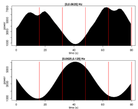
(a) Spectrogram using STFT HRV analysis.

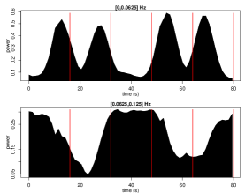
(b) Spectrogram using parametric HRV analysis.

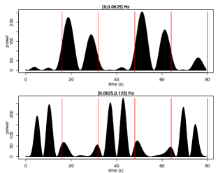
(c) Spectrogram using wavelet HRV analysis.

Figure 4: Spectrogram analysis of the simulated RR series.

Table 1: Relative power per frequency and per zone for STFT, windowed Burg method and wavelet analysis.

band$\setminus$time(s)	[0,16)	[16,32)	[32,48)	[48,64)	[64,80)
VLF	0.209	0.235	0.067	0.217	0.272
LF	0.128	0.147	0.384	0.224	0.117

(a) Fourier Analysis

band$\setminus$time(s)	[0,16)	[16,32)	[32,48)	[48,64)	[64,80)
VLF	0.180	0.245	0.083	0.259	0.233
LF	0.228	0.124	0.288	0.167	0.193

(b) Parametric Analysis

band$\setminus$time(s)	[0,16)	[16,32)	[32,48)	[48,64)	[64,80)
VLF	0.040	0.400	0.041	0.447	0.072
LF	0.270	0.071	0.344	0.077	0.238

(c) Wavelet analysis

For each of the two bands, and for each of the five zones with different spectral components, we calculated the ratio of the power that the band presents in each zone divided by the overall power of the band in the five zones. Theoretically, the power in the VLF band should be distributed among the $2^{nd}$ and $4^{th}$ zones, whereas the power in the LF band should be distributed among the $1^{st}$, $3^{rd}$ and $5^{th}$ zones. Therefore, the ideal ratios if perfect time-frequency discrimination is obtained are $(0,0.5,0,0.5,0)$ and $(1/3,0,1/3,0,1/3)$. Tables 2(a), 2(b) and 2(c) show the real ratios for the STFT, the Burg method and wavelet analysis, respectively. We can see that the wavelet ratios are closer to the theoretical values.

3.2 Computational burden

The top of Fig. 5 compares execution time (as a function of the signal size) of HRV analysis algorithms based on MODWPT, PMODWPT (our algorithm) and the STFT. The input signal to these algorithms was generated randomly. In order to compare Fourier with wavelet-based analysis, two configurations of the STFT typically used on HRV analysis were selected. First Fourier analysis used a window size and a displacement value of 5 minutes and 30 s, respectively (“Typical Fourier” in Fig. 5). The second Fourier analysis used a shorter window in order to achieve a higher temporal resolution. Window size and displacement took a value of 30 s and 2.5 s, respectively (“High Resolution Fourier” in Fig. 5). Wavelet analysis was performed using least asymmetric Daubechies of width 8 (“la8”) and extremal phase Daubechies of width 4 (“d4”) since the efficiency depends on the filter length.

PMODWPT and “Typical Fourier” STFT are much more efficient than MODWPT and “High Resolution Fourier” STFT when analyzing HRV signals (see the top of Fig. 5). The bottom of Fig. 5 shows that the performance of the PMODWPT is comparable to the “Typical Fourier” analysis.

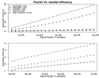
Figure 5: Performance of HRV analysis using PMODWPT, MODWPT and STFT.

3.3 Validation on real data

We have tested the algorithms presented in this paper on the recordings of the Apnea ECG database used in the PhysioNet/Computers in Cardiology Challenge 2000 [21]. Obstructive Sleep Apnea-Hypopnea (OSAH) Syndrome is a sleep-breathing disorder characterized by the presence of total (apneas) and/or partial (hypopneas) cessations of respiratory airflow while the patient is asleep. There is an interest in developing low-cost OSAH screening tests that can be carried out in the patient’s home and that can decrease the workload of hospitals’ Sleep Units. This is related to the goal of the Computers in Cardiology Challenge 2000: to develop a diagnostic test for OSAH from a single ECG lead. The dataset for this challenge is divided into a learning set and a test set. Each of these sets consist of 35 recordings of the modified lead V2 of the patient’s ECG recorded during nocturnal rest. Both training and test sets are made of 20 recordings of patients suffering from OSAH, 5 recordings of patients who were on the borderline between normality and OSAH, and 10 recordings of control patients who did not suffer from the disorder. Each recording includes minute by minute annotations indicating the presence or absence of apneas during that minute.

The goal of the second part of the challenge, the one which will be addressed here, is to detect whether or nor the patient has suffered an apnea during each minute of nocturnal rest. To this end we shall use two algorithms previously published in the bibliography which are based on the calculation of a ratio between HRV spectral power in two different bands. Specifically, we have computed the Drinnan ratio ($R_{d}$) [22] and the Otero ratio ($R_{o}$) [23]. The Drinnan ratio and the Otero ratio are defined as $R_{d}=\frac{P(\left[0.005,0.01\;Hz\right])}{P(\left[0.01,0.05\;Hz\right])}$ and $R_{o}=\frac{P(\left[0.026,0.06\;Hz\right])}{P(\left[0.06,0.25\;Hz\right])},$ respectively. Both ratios were computed with RHRV using both wavelet and Fourier analysis.

The ratios obtained for each minute of the recording were fed to a support vector machine (SVM) [24]. The SVM was trained using the learning set and validated on the validation set of the Apnea ECG Database. The scores (percentage of minutes labelled correctly) obtained in the minute by minute apnea classification using $R_{d}$, $R_{o}$ and $(R_{d},R_{o})$ as SVM parameters when the spectral power in the bands was calculated using wavelets were: 74.9%, 68.4% and 78.5%, respectively. When using Fourier, the scores were 71.4%, 66.8% and 75.4%, respectively.

Wavelet-based analysis performs slightly better than Fourier-based analysis in all scenarios. This may be due to the non-stationary nature of the signal being analyzed, and the fact that the higher temporal resolution of the wavelet analysis can help minimize the spectral contributions of apneas which have occurred outside the minute in question, but close to the end of the previous minute or to the beginning of the following one.

4 Discussion

We have presented an algorithm to perform HRV power spectrum analysis based on the MODWPT. The computational load of the our algorithm is comparable to the load of widely used STFT-based algorithms. The algorithm has been validated over simulated RR series with known spectral components. We have shown that the STFT and the windowed Burg method miss some quick changes that are successfully identified by the MODWPT. These results suggest that wavelet-based analysis is a better tool to analyze fast transient phenomena in the RR time series than other techniques based on windowing.

In order to obtain optimal temporal resolution, we should avoid descending to deep levels of the PMODWPT decomposition tree. In RHRV, a warning is generated if the band cover needed for the analysis requires expanding more than $\log_{2}(N/(L-1)+1)$ levels, $N$ being the number of samples of the signal and $L$ the filter length. A careful selection of the frequency bands to be analyzed provides some control over the depth of the tree. For example, if the RR time series is sampled at 4 Hz, and we want to obtain the power in the band $[0.27,0.5]$ Hz with a tolerance in the position of the band’s boundaries of 0.01, our algorithm will need to descend seven levels on the tree. However, to calculate the power in $[0.26,0.5]$ Hz with the same tolerance our algorithm only needs to descend three levels. In this way, we obtain a good estimate of the power in the band $[0.27,0.5]$ Hz without compromising the temporal resolution of the results.

A corollary of the phenomenon described in the previous paragraph is that, in order to achieve optimum temporal resolution (and therefore maximize the chance of identifying fast transient phenomena), the spectral bands used in HRV analysis with wavelets will probably have to differ from those traditionally associated with VLF, LF and HF. This opens the question of what may be the pathophysiological significance of spectral bands different from those which have already been widely studied in the literature.

The mother wavelet used in HRV analysis also influences the time-frequency resolution because it determines the filter shape. Further study on how the mother wavelet influences the results of the HRV analysis is required. For example, our initial tests suggest that shorter wavelets have greater time resolution than the larger wavelets, whereas the latter have a better filtering behavior than the first ones.

When performing a wavelet analysis, a careful choice of the bands is needed to avoid heavy computations, as well as a choice of the mother wavelet. When using STFT analysis we also have to choose the frequency bands (although we have more flexibility in the choice), as well as the window size, window displacement and zero padding size. Overall, more parameter choices need to be made when using the STFT. Furthermore, the selection of the STFT parameters is complex, not only because of the computation efficiency, but also because the use of a certain window size influences the temporal resolution and the frequency bands available to the analysis. To address this issue, some authors use different windows for each frequency band. This makes the analysis process heavy. Moreover, the results obtained in each of the bands are not comparable since they have been obtained using different windows. The need for tuning a lower number of knobs, and the possibility of using the same parameters in the analysis of all the HRV frequency bands are two additional advantages of using wavelets in HRV studies.

The algorithm described in this paper has been implemented in the RHRV package for the R environment in its 3.0 version. To the best of our knowledge, RHRV is the first HRV analysis toolkit that supports wavelet-based spectral analysis of the RR time series. This software can be freely downloaded from [25]. The availability of this package will enable researchers to carry out HRV power spectrum analysis based on the wavelet transform in a simple manner (see Listing 2). We hope that this will help increase the number of HRV studies that use the higher temporal resolution wavelet-based techniques.

Figure captions

• Figure 1: MODWPT decomposition tree with the nodes selected to cover the band $[0,7/16]$ Hz. $\mathbf{W}_{0,0}$ represents the original signal, $f(t).$

• Figure 2: Prune procedure using the PMODWPT. The crosses indicates which nodes have been pruned.

• Figure 3: Time shift using MODWPT without (top) and with (bottom) “Center of Energy” correction. The vertical lines indicate where spectral power should be.

• Listing 1: Pseudocode of our wavelet-based HRV analysis algorithm.

• Listing 2: HRV wavelet-based analysis in RHRV.

• Figure 4: Spectrogram analysis of the simulated RR series.

• Table 1: Relative power per frequency and per zone for STFT, windowed Burg method and wavelet analysis.

• Figure 5: Performance of HRV analysis using PMODWPT, MODWPT and STFT.

References

- Malik and Camm [1995] M. Malik, A. Camm, Heart rate variability, Futura Pub. Co., Armonk, NY, 1995.
- Jovic and Bogunovic [2012] A. Jovic, N. Bogunovic, Evaluating and comparing performance of feature combinations of heart rate variability measures for cardiac rhythm classification, Biomedical Signal Processing and Control 7 (2012) 245–255.
- Akselrod et al. [1981] S. Akselrod, D. Gordon, F. Ubel, D. Shannon, A. Berger, R. Cohen, Power spectrum analysis of heart rate fluctuation: a quantitative probe of beat-to-beat cardiovascular control, Science 213 (1981) 220.
- Lewis et al. [2007] M. J. Lewis, M. Kingsley, A. Short, K. Simpson, Influence of high-frequency bandwidth on heart rate variability analysis during physical exercise, Biomedical Signal Processing and Control 2 (2007) 34–39.
- tas [1996] Heart rate variability: standards of measurement, physiological interpretation and clinical use. Task Force of the European Society of Cardiology and the North American Society of Pacing and Electrophysiology., Circulation 93 (1996) 1043–1065.
- Vila et al. [1997] J. Vila, F. Palacios, J. Presedo, M. Fernandez-Delgado, P. Felix, S. Barro, Time-frequency analysis of heart-rate variability, Engineering in Medicine and Biology Magazine, IEEE 16 (1997) 119–126.
- Mallat [1989] S. Mallat, A theory for multiresolution signal decomposition: The wavelet representation, IEEE Transactions on Pattern Analysis and Machine Intelligence 11 (1989) 674–693.
- kub [2012] Kubios HRV, Heart Rate Variability Analysis Software, biosignal Analysis and Medical Imaging Group, University of Eastern Finland, http://kubios.uef.fi/, website last accessed February 2012.
- ahr [2012] Nevrokard-aHRV software, http://www.nevrokard.eu/index.html, website last accessed February 2012.
- Addison [2005] P. S. Addison, Wavelet transforms and the ecg: a review, Physiological measurement 26 (2005) R155.
- Hossen and Al-Ghunaimi [2007] A. Hossen, B. Al-Ghunaimi, A wavelet-based soft decision technique for screening of patients with congestive heart failure, Biomedical Signal Processing and Control 2 (2007) 135–143.
- García et al. [2012] C. García, A. Otero, X. Vila, M. Lado, An open source tool for heart rate variability wavelet-based spectral analysis, in: International Joint Conference on Biomedical Engineering Systems and Technologies, BIOSIGNALS 2012, pp. 206–211.
- Mallat [1999] S. Mallat, A wavelet tour of signal processing. Second Edition, Academic Pr, 1999.
- Percival and Walden [2006] D. Percival, A. Walden, Wavelet methods for time series analysis, volume 4, Cambridge Univ Pr, 2006.
- Gabor [1946] D. Gabor, Theory of communication. part 1: The analysis of information, Journal of the Institution of Electrical Engineers-Part III: Radio and Communication Engineering 93 (1946) 429–441.