11institutetext: Department of Physics, Harbin Institute of Technology, Harbin 150001, China 22institutetext: Center for Quantum Sciences and School of Physics, Northeast Normal University, Changchun 130024, China 33institutetext: Department of Physics, College of Science, Yanbian University, Yanji, Jilin 133002, China

Preparation of entanglement between atoms in spatially separated cavities via fiber loss

Shi-Lei Su 11    Xiao-Qiang Shao 22    Qi Guo 11    Liu-Yong Cheng 11    Hong-Fu Wang 33    Shou Zhang Corresponding author: szhang@ybu.edu.cn1133
(Received: date / Revised version: date)
Abstract

We propose a scheme to prepare a maximally entangled state for two $\Lambda$-type atoms trapped in separate optical cavities coupled through an optical fiber based on the combined effect of the unitary dynamics and the dissipative process. Our work shows that the fiber loss, as well as the atomic spontaneous emission and the cavity decay, is no longer undesirable, but requisite to prepare the distributed entanglement, which is meaningful for the long distance quantum information processing tasks. Originating from an arbitrary state, the desired state could be prepared without precise time control. The robustness of the scheme is numerically demonstrated by considering various parameters.

pacs:
03.67.BgEntanglement production and manipulation and 42.50.PqCavity quantum electrodynamics; micromasers and 03.65.Yz Decoherence; open systems; quantum statistical methods

1 Introduction

Quantum entanglement w001 ; w002 is a fundamental and fascinating quantum effect and has been a key resource for quantum information science (QIS) w003 ; w004 ; w005 . How to effectively prepare entanglement influences the development of QIS. One traditional obstacle for preparing entanglement is the dissipation that induced by the inevitable coupling between the quantum system and the environment, which would degrade the quantum coherence of the system. The usual methods to deal with the dissipation can be divided into the following categories: quantum error correction w006 ; w007 ; w008 , decoherence-free subspace w009 ; w010 ; w011 , geometric phase w012 ; w013 ; w014 ; w015 , quantum-control technique w016 ; w017 ; w018 and dissipative dynamics  w019 ; w020 ; w021 ; w022 ; w023 ; w024 ; w025 ; w026 ; w027 ; w028 ; w029 ; w030 ; w031 ; w032 ; w033 ; w034 ; w035 ; w036 ; w037 ; w038 ; w039 ; w040 ; w043 ; w044 ; w045 ; w048 ; b048 ; w041 ; w042 ; w046 ; w047 ; b049 ; b050 ; nb051 . Compared with the other methods, dissipative dynamics has unique characters since the dissipation is used to prepare entanglement so that the preparation process is robust against decoherence. In particular, Kastoryano et al. considered a dissipative scheme for preparing a maximally entangled state of two $\Lambda$-type atoms trapped in one optical cavity w030 , whose performance is better than that based on the unitary dynamics. Subsequently, this scheme was generalized to coupled cavity system w035 , atom-cavity-fiber system w037 and the circuit quantum electrodynamics system w044 . Besides, Zheng et al. proposed two schemes to prepare the maximal entanglement between two atoms coupled to a decaying resonator w048 ; b048 . The common place of these schemes is that the cavity decay is used as resource for state preparation. On the other hand, Rao and Mølmer, Carr and Saffman considered two schemes w041 ; w042 to prepare the entanglement of Rydberg atoms via dissipation, respectively. And Shao et al. gave two dissipative schemes for three-dimensional entanglement preparation w046 ; w047 . These schemes demonstrated that the atomic spontaneous emission is quite capable of being the powerful resource for entanglement preparation. Moreover, the schemes proposed in Refs. w031 ; b049 indicate that the atomic spontaneous emission and cavity decay could be used simultaneously to prepare the desired entanglement for two atoms in one cavity.

To realize the long distance and large-scale quantum information processing, atom-cavity-fiber system is proposed w049 ; w050 and has been an excellent platform for distributed quantum computation w051 ; w052 , quantum entanglement preparation  w053 ; w054 ; w055 ; w056 ; w057 ; w058 , and quantum communication w059 . For these unitary-dynamics-based schemes, atomic spontaneous emission, cavity decay and the fiber loss are three main and undesirable dissipative factors, which would affect the practical applications of the scheme in the QIS.

The previous dissipative schemes showed that the atomic spontaneous emission or cavity decay is no longer undesirable, but necessary for maximal entanglement preparation for two atoms trapped in one cavity. In this paper, we generalize the idea to the case when two atoms trapped into two distributed cavities that connected through an optical fiber. Interestingly, we find that the fiber loss, like the other two dissipative factors, could also be used to prepare the distributed entanglement, which is meaningful for the long distance and large-scale quantum information processing tasks. The present work has the following features: (i) It has no specific requirement of the initial state. (ii) It does not need to control evolution time accurately. And, it is robustness on parameter fluctuations. (iii) Different with the unitary-dynamics-based schemes in the atom-cavity-fiber system, the present one shows that, the fiber loss, as well as the atomic spontaneous emission and the cavity decay, is no longer undesirable, but requisite for the preparation of the distributed entanglement. (iv) In contrast with the schemes based on the similar system w037 ; w038 , the current one is special in the sense that the decay of cavity and fiber modes are considered uncorrelated since we do not define the normal bosonic mode $\hat{c}$ to rewrite the Hamiltonian.

2 Fundamental model

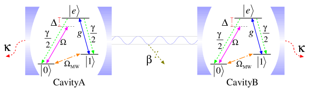
We consider the setup described in Fig. 1, where two identical $\Lambda$-type atoms are individually trapped into two single mode cavities coupled through an optical fiber with length l. Each atom has two ground states $|0\rangle$ and $|1\rangle$ and one excited state $|e\rangle$ with the corresponding energies $\omega_{0}$, $\omega_{1}$ and $\omega_{e}$, respectively. The atomic transition $|1\rangle\leftrightarrow|e\rangle$ is coupled resonantly to the corresponding cavity mode with the coupling constant $g$. Besides, the transition $|0\rangle\leftrightarrow|e\rangle$ is driven by the corresponding off-resonance optical laser with detuning $\Delta$, and Rabi frequency $\Omega$. The transition between two ground states $|0\rangle$ and $|1\rangle$ is coupled resonantly by means of a microwave field with Rabi frequency $\Omega_{\rm MW}$. In the short fiber limit $(l\bar{v})/(2\pi c)\leqslant 1$, where $\bar{v}$ is the decay rate of the cavity fields into a continuum of fiber modes, only one fiber mode interacts with the cavity mode w050 ; w051 ; w052 . For simplicity, we assume the interaction between cavity mode and fiber mode is resonant. Under the rotating wave approximation, the Hamiltonian of the whole system could be written as (setting $\hbar=1$) $H=H_{a,c,f}+H_{cl}+H_{mw}$,

$\displaystyle H_{a,c,f}$ $\displaystyle=$ $\displaystyle\sum_{i={\rm A,B}}\Big{[}\sum_{j=0,1,e}\omega_{j}|j\rangle_{ii}\langle j|+\omega_{a}a^{{\dagger}}_{i}a_{i}$ (5)
$\displaystyle+~{}~{}(g|e\rangle_{ii}\langle 1|a_{i}+{\rm H.c.})\Big{]}$
$\displaystyle+~{}~{}\omega_{b}b^{{\dagger}}b+\big{[}\nu b(a^{{\dagger}}_{A}+a^{{\dagger}}_{B})+{\rm H.c.}\big{]},$
$$H_{cl}=\Omega\sum_{i={\rm A,B}}e^{i\omega t}|0\rangle_{ii}\langle e|+{\rm H.c.},$$ (6)
$$H_{mw}=\Omega_{\rm MW}e^{i\omega_{\rm MW}t}(|0\rangle_{\rm AA}\langle 1|-|0\rangle_{\rm BB}\langle 1|)+{\rm H.c.},$$ (7)

in which $a_{i}$ and $a^{{\dagger}}_{i}$ denote the annihilation and creation operators for the optical mode of cavity i, respectively. $b$ and $b^{{\dagger}}$ denote the annihilation and creation operator for the fiber mode, respectively. $\omega_{a}$ and $\omega_{b}$ denote the frequencies of cavity mode and the fiber mode, respectively. $\omega$ and $\omega_{\rm MW}$ stand for the frequencies of the classical laser field and the microwave field, respectively. $\nu$ is the coupling strength between the cavity mode and the fiber mode.

Refer to caption
Figure 1: Experimental setup and level diagram of $\Lambda$-type atoms. $\gamma$, $\kappa$ and $\beta$ denote the atomic spontaneous emission rate, cavity decay rate and fiber loss rate, respectively. Here, we assume the cavity decay rate of the two cavities are the same, and the excited state $|e\rangle$ spontaneously decays into two ground states with branching rate $\gamma/2$.

Then, we define the excitation number operator of the total system $N_{e}=\sum_{i=\rm A,B}(|e\rangle_{ii}\langle e|+a^{{\dagger}}_{i}a_{i})+b^{{\dagger}}b$. Under the weak excitation condition and if the initial state is in the zero excitation subspace, we can safely discard the subspace with excitation number greater than or equals two.

With the dissipation being included, the dynamics of the system in Lindblad form could be described by the master equation

$$\dot{\rho}=i[\rho,H]+\sum_{j}\Big{[}L_{j}\rho\L_{j}^{{\dagger}}-\frac{1}{2}(\L_{j}^{{\dagger}}L_{j}\rho+\rho\L_{j}^{{\dagger}}L_{j})\Big{]},$$ (8)

where $L_{j}$ is the so-called Lindblad operators governing dissipation. Specifically, in the current scheme the Lindblad operators can be expressed as $L_{\beta}=\sqrt{\beta}b$, $L_{\gamma_{\rm 1}}=\sqrt{\gamma/2}|0\rangle_{\rm AA}\langle e|$, $L_{\gamma_{\rm 2}}=\sqrt{\gamma/2}|1\rangle_{\rm AA}\langle e|$, $L_{\gamma_{3}}=\sqrt{\gamma/2}|0\rangle_{\rm BB}\langle e|$, $L_{\gamma_{4}}=\sqrt{\gamma/2}|1\rangle_{\rm BB}\langle e|$, $L_{\kappa_{1}}=\sqrt{\kappa}a_{\rm A}$ and $L_{\kappa_{2}}=\sqrt{\kappa}a_{\rm B}$. $L_{\beta}$ describes the dissipation induced by the fiber loss. $L_{\gamma_{\rm 1}}$ and $L_{\gamma_{\rm 2}}$ describe the dissipation induced by the spontaneous emission of atom in cavity A. $L_{\gamma_{\rm 3}}$ and $L_{\gamma_{\rm 4}}$ describe the dissipation induced by the spontaneous emission of atom in cavity B. $L_{\kappa_{1}}=\sqrt{\kappa}a_{\rm A}$ and $L_{\kappa_{2}}=\sqrt{\kappa}a_{\rm B}$ describe the dissipation induced by the leakage of cavities A and B, respectively. Since cavity A and cavity B are distant from each other, the dissipation processes are spatially separated.

3 Preparation of the distributed entanglement

3.1 Dressed states

To see clearly the roles of the classical laser field, microwave field and dissipative factors, we identify the eigenstates of the Hamiltonian $H_{a,c,f}$ in zero and one excitation subspace and use them as dressed states.

Table 1: The eigenstates and the corresponding eigenenergies of Hamiltonian $H_{a,c,f}$ in zero excitation subspaces. Here, $|\alpha\beta\rangle|\gamma\delta\epsilon\rangle$ represents that atom in cavity A (B) is in the state $|\alpha\rangle$ ($|\beta\rangle$), optical mode of the cavity A (B) is in the state $|\gamma\rangle~{}(|\epsilon\rangle)$ and of the fiber is in state $|\delta\rangle$.
Eigenstate Eigenenergy
$|00\rangle|000\rangle$ 0
$|S\rangle|000\rangle$ $\omega_{1}$
$|T\rangle|000\rangle$ $\omega_{1}$
$|11\rangle|000\rangle$ 2$\omega_{1}$
Table 2: The eigenstates and the corresponding eigenenergies of Hamiltonian $H_{a,c,f}$ in one excitation subspace.
Eigenstate Eigenenergy
$|\varphi\rangle_{1}$ $\omega_{e}-\omega_{1}$
$|\varphi\rangle_{2}$ $\omega_{e}-\omega_{1}-\sqrt{2}\nu$
$|\varphi\rangle_{3}$ $\omega_{e}-\omega_{1}+\sqrt{2}\nu$
$|\varphi\rangle_{4}$ $\omega_{e}+\omega_{1}$
$|\varphi\rangle_{5}$ $\omega_{e}+\omega_{1}-g$
$|\varphi\rangle_{6}$ $\omega_{e}+\omega_{1}+g$
$|\varphi\rangle_{7}$ $\omega_{e}+\omega_{1}-g_{1}$
$|\varphi\rangle_{8}$ $\omega_{e}+\omega_{1}+g_{1}$
$|T_{1}\rangle$, $|S_{1}\rangle$ $\omega_{e}-\sqrt{g_{1}^{2}-g_{3}^{2}}/\sqrt{2}$
$|T_{2}\rangle$, $|S_{2}\rangle$ $\omega_{e}+\sqrt{g_{1}^{2}-g_{3}^{2}}/\sqrt{2}$
$|T_{3}\rangle$, $|S_{3}\rangle$ $\omega_{e}-\sqrt{g_{1}^{2}+g_{3}^{2}}/\sqrt{2}$
$|T_{4}\rangle$, $|S_{4}\rangle$ $\omega_{e}+\sqrt{g_{1}^{2}+g_{3}^{2}}/\sqrt{2}$

In Tables 1 and 2, we show the eigenstates and the corresponding eigenvalues (setting $\omega_{0}$=0) with the notations shown in Appendix, and $|T\rangle$ is the maximal entanglement we want to prepare for the two distributed atoms.

3.2 Roles of the microwave field and the classical laser field

Refer to caption
Figure 2: Level configuration and the transitions of the states in the dressed state picture. Microwave field causes resonant transitions among states $|11\rangle|000\rangle$, $|S\rangle|000\rangle$ and $|00\rangle|000\rangle$. Classical laser field causes resonant transitions between states $|00\rangle|000\rangle$ and $|T_{4}\rangle$. The other transitions between state in zero excitation subspace and that in one excitation caused by classical laser field are non-resonant with different detunings. Dissipative factors, i.e., atomic spontaneous emission, cavity decay and fiber loss, are critical to translate the state $|T_{4}\rangle$ into the desired state. We use the notations $\Omega_{1}=\sqrt{2}g\nu\Omega/\sqrt{g_{3}^{4}+g^{2}g_{3}^{2}-2\nu^{2}g_{3}^{2}}$ and $\Omega_{2}=\sqrt{2}g\nu\Omega/\sqrt{g_{3}^{4}-g^{2}g_{3}^{2}+2\nu^{2}g_{3}^{2}}$ for simplicity.

Under the dressed state picture, Hamiltonian $H_{mw}$ can be rewritten as

$\displaystyle H_{mw}$ $\displaystyle=$ $\displaystyle\sqrt{2}~{}\Omega_{\rm MW}~{}e^{i\omega_{\rm MW}t}(|S\rangle|000\rangle\langle 000|\langle 11|$ (11)
$\displaystyle-|00\rangle|000\rangle\langle 000|\langle S|){\rm+~{}H.c.}.$

Similarly, $H_{cl}$ can be rewritten as

$\displaystyle H_{cl}$ $\displaystyle=$ $\displaystyle\frac{\sqrt{2}g\nu\Omega}{\sqrt{g_{3}^{4}+g^{2}g_{3}^{2}-2\nu^{2}g_{3}^{2}}}e^{i\omega t}|00\rangle|000\rangle(\langle T_{1}|+\langle T_{2}|)$ (20)
$\displaystyle+\frac{\sqrt{2}g\nu\Omega}{\sqrt{g_{3}^{4}-g^{2}g_{3}^{2}+2\nu^{2}g_{3}^{2}}}e^{i\omega t}|00\rangle|000\rangle(\langle T_{3}|+\langle T_{4}|)$
$\displaystyle+\frac{\sqrt{2}\Omega\nu}{g_{1}}e^{i\omega t}|T\rangle|000\rangle\langle\varphi_{4}|$
$\displaystyle+\frac{g\Omega}{\sqrt{2}g_{1}}e^{i\omega t}|T\rangle|000\rangle(\langle\varphi_{7}|+\langle\varphi_{8}|)$
$\displaystyle+\frac{\Omega}{\sqrt{2}}e^{i\omega t}|S\rangle|000\rangle(\langle\varphi_{5}|+\langle\varphi_{6}|)+{\rm H.c.}.$

In the interaction picture with respect to the Hamiltonian $H_{a,c,f}$ that expressed by the eigenvectors and eigenvalues in zero and one excitation subspace, Eqs. (11) and (20) can be transformed to

$\displaystyle H_{mw}$ $\displaystyle=$ $\displaystyle\sqrt{2}~{}\Omega_{\rm MW}(|S\rangle|000\rangle\langle 000|\langle 11|-|00\rangle|000\rangle\langle 000|\langle S|)$ (23)
$\displaystyle{\rm+~{}H.c.}$

and

$\displaystyle H_{cl}$ $\displaystyle=$ $\displaystyle\frac{\sqrt{2}g\nu\Omega}{\sqrt{g_{3}^{4}+g^{2}g_{3}^{2}-2\nu^{2}g_{3}^{2}}}\Big{[}e^{i(\omega-\omega_{e}+\sqrt{g_{1}^{2}-g_{3}^{2}}/\sqrt{2})t}$ (40)
$\displaystyle\times|00\rangle|000\rangle\langle T_{1}|+e^{i(\omega-\omega_{e}-\sqrt{g_{1}^{2}-g_{3}^{2}}/\sqrt{2})t}|00\rangle|000\rangle\langle T_{2}|\Big{]}$
$\displaystyle+\frac{\sqrt{2}g\nu\Omega}{\sqrt{g_{3}^{4}-g^{2}g_{3}^{2}+2\nu^{2}g_{3}^{2}}}\Big{[}e^{i(\omega-\omega_{e}+\sqrt{g_{1}^{2}+g_{3}^{2}}/\sqrt{2})t}$
$\displaystyle\times|00\rangle|000\rangle\langle T_{3}|+e^{i(\omega-\omega_{e}-\sqrt{g_{1}^{2}+g_{3}^{2}}/\sqrt{2})t}|00\rangle|000\rangle\langle T_{4}|\Big{]}$
$\displaystyle+\frac{\sqrt{2}\Omega\nu}{g_{1}}e^{i(\omega-\omega_{e})t}|T\rangle|000\rangle\langle\varphi_{4}|$
$\displaystyle+\frac{g\Omega}{\sqrt{2}g_{1}}\Big{[}e^{i(\omega-\omega_{e}+g_{1})t}|T\rangle|000\rangle\langle\varphi_{7}|$
$\displaystyle+e^{i(\omega-\omega_{e}-g_{1})t}|T\rangle|000\rangle\langle\varphi_{8}|\Big{]}$
$\displaystyle+\frac{\Omega}{\sqrt{2}}\Big{[}e^{i(\omega-\omega_{e}+g)t}|S\rangle|000\rangle\langle\varphi_{5}|$
$\displaystyle+e^{i(\omega-\omega_{e}-g)t}|S\rangle|000\rangle\langle\varphi_{6}|\Big{]}+{\rm H.c.}.$

Equation. (23) shows that Hamiltonian $H_{mw}$ causes resonant transitions among states $|11\rangle|000\rangle$, $|S\rangle|000\rangle$ and $|00\rangle|000\rangle$, as we shall see later, which is exactly the reason why the scheme is independent of the initial states. From Eq. (40), one can see that classical laser field causes interactions between the states in zero excitation subspace and that in one excitation subspace, and the detuning of the interaction could be adjusted through choosing the values of $\omega$, $\omega_{e}$, $g$ and $\nu$ according to the requirement of the scheme. For example, if one choose $\omega_{e}-\omega=-\sqrt{g_{1}^{2}+g_{3}^{2}}/\sqrt{2}$, $|00\rangle|000\rangle$ would couple resonantly to $|T_{4}\rangle$, while other terms in Eq. (40) would undergo non-resonant interactions with different detunings.

3.3 Roles of the dissipative factors

Dissipation, which can occur via the fiber loss, atomic spontaneous emission, and cavity decay, is an integrant component of the current state preparation scheme. The states in one excitation subspace would be transformed to the corresponding states in zero excitation subspace via dissipation. Interestingly, it is easy to find that the second term of $|T_{4}\rangle$ would be transformed to the state $|T\rangle|000\rangle$ (have not considered the normalization factor) when $L_{\beta}$ works. The first and the third terms of $|T_{4}\rangle$ would be transformed to the state $|T\rangle|000\rangle$ when $L_{\kappa_{1}}$ and $L_{\kappa_{2}}$ work. Besides, the fourth term of $|T_{4}\rangle$ would also be converted to $|T\rangle|000\rangle$ when $L_{\gamma_{2}}$ and $L_{\gamma_{4}}$ work. Since $|T\rangle|000\rangle$ is the product state of the atomic maximally entangled state $|T\rangle$, the cavity mode vacuum state, and the fiber mode vacuum state, the scheme would be considered successful if $|T\rangle|000\rangle$ is prepared. Therefore, in order to prepare the desired state, it is better if other undesired states in zero excitation subspace could be coupled resonantly to $|T_{4}\rangle$ in one excitation subspace directly or indirectly.

3.4 Preparation process
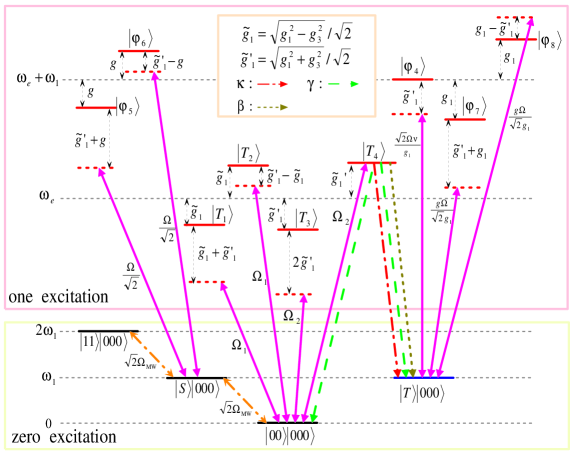
Refer to caption
Figure 3: (a)(c)(e) Populations of the states in zero subspace with the initial state $|11\rangle|000\rangle$. (b)(d)(f) Fidelities of the desired state with the initial state $|11\rangle|000\rangle$. In subfigures (a) and (b), the parameters are chosen as $\Omega=0.008g,\Omega_{\rm MW}=0.25\Omega,\nu=g$. And the dissipative factors are chosen as $\beta=0.1g$, $\kappa=0$, and $\gamma=0$. The inset of subfigure (b) is plotted with the dissipative factors $\kappa=0$, $\gamma=0$, and $\beta$ varies from 0 to $0.1g$ at the time $8\times 10^{3}/g$. In subfigures (c) and (d), the parameters are chosen as $\Omega=0.008g,\Omega_{\rm MW}=0.2\Omega,\nu=g$. And the dissipative factors are chosen as $\beta=0$, $\kappa=0.1g$, and $\gamma=0$. The inset of subfigure (d) is plotted with the dissipative factors $\beta=0$, $\gamma=0$, and $\kappa$ varies from 0 to $0.1g$ at the time $1.6\times 10^{4}/g$. In subfigures (e) and (f), the parameters are chosen as $\Omega=0.008g,\Omega_{\rm MW}=0.2\Omega,\nu=g$. And the dissipative factors are chosen as $\beta=0$, $\kappa=0$, and $\gamma=0.1g$. The inset of subfigure (f) is plotted with the dissipative factors $\beta=0$, $\kappa=0$, and $\gamma$ varies from 0 to $0.1g$ at the time $1.6\times 10^{4}/g$.

If the parameters satisfy $\omega_{e}-\omega=-\sqrt{g_{1}^{2}+g_{3}^{2}}/\sqrt{2}$, $|00\rangle|000\rangle$ would couple resonantly to $|T_{4}\rangle$ while the other terms in Eq. (40) underdo non-resonant interactions with different detunings. First, we take into account the case that the initial state is $|11\rangle|000\rangle$. As shown in Sec. 3.2, $|11\rangle|000\rangle$ would be transformed to $|00\rangle|000\rangle$ through the intermediate state $|S\rangle|000\rangle$. Since $|00\rangle|000\rangle$ couples resonantly to $|T_{4}\rangle$, the initial state $|11\rangle|000\rangle$ would be transformed to $|T\rangle|000\rangle$ via dissipation finally. The process could be expressed as $~{}~{}~{}~{}|11\rangle|000\rangle\xrightarrow[]{H_{mw}}|S\rangle|000\rangle\xrightarrow[]{H_{mw}}|00\rangle|000\rangle\xrightarrow[]{H_{cl}}|T_{4}\rangle\xrightarrow[]{\gamma,\kappa,\beta}|T\rangle|000\rangle$. Similarly, if the initial state is $|S\rangle|000\rangle$ or $|00\rangle|000\rangle$, it would also be converted to the desired state finally. Besides, since $|01\rangle|000\rangle$ or $|10\rangle|000\rangle$ could be regarded as a superposition of the states $|S\rangle|000\rangle$ and $|T\rangle|000\rangle$, and $|S\rangle|000\rangle$ would be transformed to $|T\rangle|000\rangle$ finally, the desired state could also be achieved if the initial state is $|01\rangle|000\rangle$ or $|10\rangle|000\rangle$. In brief, if the initial state is $|T\rangle|000\rangle$, it is stable and keeps invariant. Otherwise, it would be transformed to $|T\rangle|000\rangle$ via unitary dynamics and dissipative process. As a result, the population of $|T\rangle|000\rangle$ accumulates as time grows.

In the above analysis, for simplicity we only consider the dissipative channel $|e\rangle\rightarrow|1\rangle$ when we study the roles of the atomic spontaneous emission. Nevertheless, the atomic spontaneous emission has another possibilities, $|e\rangle\rightarrow|0\rangle$. By the time that happens, the fourth term of the state $|T_{4}\rangle$ would be converted to $|00\rangle|000\rangle$, which is coupled resonantly to the state $|T_{4}\rangle$ through the classical laser field and thus has little or no effect on the state preparation. The detailed level configuration and the transformed process of the whole scheme are shown in Fig. 2.

We also noticed that $|T_{1}\rangle$, $|T_{2}\rangle$, and $|T_{3}\rangle$ could also be transformed to the desired state through the dissipative process. Thus, if the selection of $\omega_{e}-\omega$ could realize the resonant interactions between the state $|00\rangle|000\rangle$ and any one of the three states $|T_{1}\rangle$, $|T_{2}\rangle$ and $|T_{3}\rangle$, the desired state could also be prepared via the dissipation.

4 Discussion

Refer to caption
Figure 4: Fidelity of the desired state with the initial state $|11\rangle|000\rangle$ at the time $1.5\times 10^{4}/g$. The parameters are chosen as $\Omega=0.008g,\Omega_{\rm MW}=0.25\Omega$, and $\nu=g$. (a) The dissipative factors $\beta$ and $\kappa$ vary from 0 to $0.06g$, and $\gamma$ is set to zero. (b) The dissipative factors $\beta$ and $\gamma$ vary from 0 to $0.06g$, and $\kappa$ is set to zero. (c) The dissipative factors $\gamma$ and $\kappa$ vary from 0 to $0.06g$, and $\beta$ is set to zero.
Refer to caption
Figure 5: Fidelity of the desired state with the initial state $|11\rangle|000\rangle$. The parameters are chosen as $\Omega=0.008g,\Omega_{\rm MW}=0.25\Omega$, and $\nu=g$. The dissipative factors are set as $\beta=\kappa=\gamma$.
Refer to caption
Figure 6: (a) Fidelity of the desired state versus the relative fluctuations of $\Omega$ and $\Omega_{\rm MW}$ with the initial state $|11\rangle|000\rangle$ at the time $2\times 10^{4}/g$. The notations d$\Omega$ and d$\Omega_{\rm MW}$ in the axis labels denote the deviations of $\Omega$ and $\Omega_{\rm MW}$, respectively. The parameters are chosen as $\Omega=0.008g,\Omega_{\rm MW}=0.002g$, and $\nu=g$. (b) Fidelity of the desired state versus $\nu$ and evolution time with the initial state $|11\rangle|000\rangle$. The parameters are chosen as $\Omega=0.008g$ and $\Omega_{\rm MW}=0.002g$. Both figures are plotted with the dissipative factors $\beta=\kappa=\gamma=0.04g$.

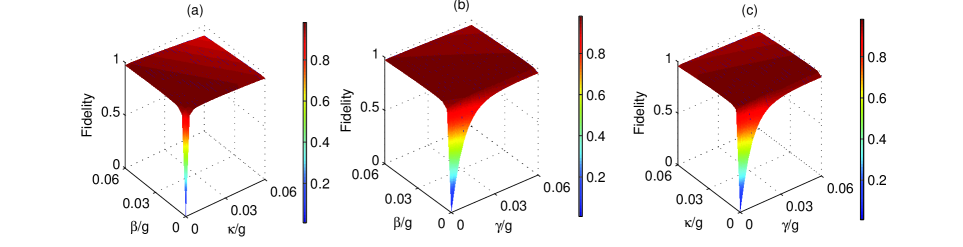
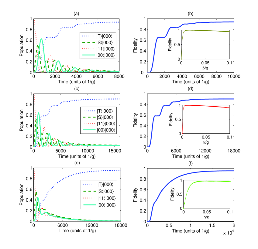
To verify the feasibility of the scheme, we solve the master equation numerically in zero and one excitation subspace. For the purpose of studying the effect of each of the dissipative factors, we would first consider one factor at a time. Then, the combined effect of the dissipative factors would be considered. In Figs. 3(a) and 3(b), we plot the populations and the fidelity of the scheme when the dissipative factors satisfy $\beta=0.1g$, $\kappa=0$, and $\gamma=0$. The results show that the desired state could be prepared with the fidelity more than 94% when the evolution time equals $10^{4}/g$. The inset in Fig. 3(b) shows that when $\kappa=\gamma=0$, the fiber loss is critical for the state preparation since the fidelity would be zero if the fiber loss is not exist. Similarly, numerical results in Figs. 3(c) and 3(d), and  3(e) and 3(f) indicate that the cavity decay and atomic spontaneous emission could also be utilized as resources to prepare the maximal entanglement with high fidelity, respectively. In Fig. 4, we plot the fidelity when two out of three dissipative factors are considered at the same time. The result gives a further verification that each of the dissipative factors could be utilized to prepare the distributed entanglement.

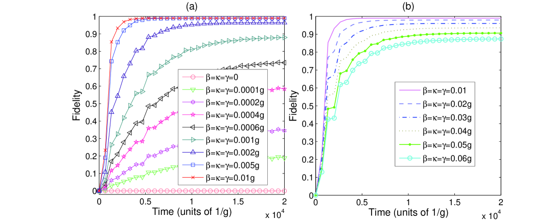
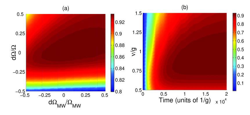
In Fig. 5, we plot the fidelity when the three dissipative factors are considered at the same time. One can see from Fig. 5(a) that the fidelity increases as the dissipative factors increases. However, as shown in Fig. 5(b), further increase of the dissipative factors would decrease the performance of the scheme. In fact, like most of the dissipative schemes, the present one is based on the combined effect of the unitary dynamics and the dissipative process. When the values of the dissipative factors are set to zero, the scheme would not succeed. As the dissipative factors increases, the role of the dissipative process becomes evident and the fidelity increases. Nevertheless, further increase of the dissipative factors would lead to an adverse effect on the unitary dynamics and thus decrease the overall performance of the scheme. Besides, in Fig. 6(a) we plot the fidelity versus the fluctuations of $\Omega$ and $\Omega_{\rm MW}$, which shows that the scheme is robust on the variation of $\Omega$ and $\Omega_{\rm MW}$ since the fidelity remains higher than 80% even when the relative errors of these two factors reach 50% simultaneously. And Fig. 6(b) indicates that the scheme is robust on the variation of the coupling strength between the cavity mode and the fiber mode.

If we use the experimental cavity-parameters $(g,\kappa,\gamma)\sim 2\pi\times(34,4.1,3.6)$MHz b060 and select $\Omega=0.015g,\Omega_{\rm MW}=0.36\Omega,\beta\simeq\kappa$, and $\nu=0.9g$ for simulation, the fidelity is about 71.7%. And this value may further decrease after considering various realistic experimental conditions. Nevertheless, as shown in Fig. 5(b), the performance can be greatly improved as the dissipative rate decreases within a certain range. Thus, a better cavity with high cooperativity should be satisfied for implementing the scheme experimentally. In addition, the short fiber limit $l\bar{\nu}/2\pi c<1$ should be fulfilled during the whole experimental process. On that premise, the scheme has certain requirements about the value of $\bar{\nu}$ for realizing long-distance quantum information processing.

In contrast with the unitary-dynamics-based schemes w053 ; w054 ; w055 ; w056 ; w057 ; w058 ; w060 , the fiber loss takes on a new role since it constitutes a vital passage from the state in one excitation subspace to the desired state in the zero excitation subspace. In comparison with the dissipative schemes w037 ; w038 based on the similar system, the difference is that the current scheme has not introduced the normal bosonic modes. Therefore, the bosonic modes of the cavity and the fiber are considered to be completely uncorrelated in our scheme.

5 Conclusion

In conclusion, we have designed an alternative scheme to prepare the distributed entanglement in the atom-cavity-fiber system via the fiber loss as well as the atomic spontaneous emission and cavity decay. And the dissipation is an essential part of the scheme. We hope that out work may be useful for the distributed quantum information processing tasks in the near future.

Appendix

$\displaystyle|S\rangle$ $\displaystyle\equiv$ $\displaystyle(|01\rangle-|10\rangle)/\sqrt{2},~{}~{}|T\rangle\equiv(|01\rangle+|10\rangle)/\sqrt{2},~{}~{}$ (41)
$\displaystyle|\varphi\rangle_{1}$ $\displaystyle\equiv$ $\displaystyle(|00\rangle|100\rangle-|00\rangle|001\rangle)/\sqrt{2},$ (43)
$\displaystyle|\varphi\rangle_{2}$ $\displaystyle\equiv$ $\displaystyle(|00\rangle|100\rangle+|00\rangle|001\rangle-\sqrt{2}|00\rangle|010\rangle)/2,~{}~{}$ (45)
$\displaystyle|\varphi\rangle_{3}$ $\displaystyle\equiv$ $\displaystyle(|00\rangle|100\rangle+|00\rangle|001\rangle+\sqrt{2}|00\rangle|010\rangle)/2,$ (47)
$\displaystyle|\varphi\rangle_{4}$ $\displaystyle\equiv$ $\displaystyle(|e1\rangle|000\rangle+|1e\rangle|000\rangle-\frac{g}{\nu}|11\rangle|010\rangle)/\sqrt{2+(\frac{g}{\nu})^{2}},$ (49)
$\displaystyle|\varphi\rangle_{5}$ $\displaystyle\equiv$ $\displaystyle(|11\rangle|001\rangle+|e1\rangle|000\rangle-|1e\rangle|000\rangle-|11\rangle|100\rangle)/2,$ (51)
$\displaystyle|\varphi\rangle_{6}$ $\displaystyle\equiv$ $\displaystyle(|11\rangle|100\rangle+|e1\rangle|000\rangle-|1e\rangle|000\rangle-|11\rangle|001\rangle)/2,$ (53)
$\displaystyle|\varphi\rangle_{7}$ $\displaystyle\equiv$ $\displaystyle(|e1\rangle|000\rangle+|1e\rangle|000\rangle+\frac{2\nu}{g}|11\rangle|010\rangle-\frac{g_{1}}{g}|11\rangle|001\rangle$ (57)
$\displaystyle-\frac{g_{1}}{g}|11\rangle|100\rangle)/\sqrt{2(\frac{g_{1}}{g})^{2}+(\frac{2\nu}{g})^{2}+2},$
$\displaystyle|\varphi\rangle_{8}$ $\displaystyle\equiv$ $\displaystyle(|e1\rangle|000\rangle+|1e\rangle|000\rangle+\frac{2\nu}{g}|11\rangle|010\rangle+\frac{g_{1}}{g}|11\rangle|001\rangle$ (61)
$\displaystyle+\frac{g_{1}}{g}|11\rangle|100\rangle)/\sqrt{2(\frac{g_{1}}{g})^{2}+(\frac{2\nu}{g})^{2}+2},$
$\displaystyle|T_{1}\rangle$ $\displaystyle\equiv$ $\displaystyle\Big{[}\frac{\sqrt{g^{2}_{1}-g^{2}_{3}}~{}(g^{2}+g^{2}_{3})}{2\sqrt{2}g\nu^{2}}(|01\rangle|100\rangle+|10\rangle|001\rangle)$ (69)
$\displaystyle-\frac{g^{2}_{2}+g^{2}_{3}}{2g\nu}(|01\rangle|010\rangle+|10\rangle|010\rangle)$
$\displaystyle-\frac{\sqrt{g^{2}_{1}-g_{3}^{2}}}{\sqrt{2}g}(|01\rangle|001\rangle+|10\rangle|100\rangle)$
$\displaystyle+(|0e\rangle|000\rangle+|e0\rangle|000\rangle)\Big{]}/\frac{\sqrt{2(g_{3}^{4}+g^{2}g_{3}^{2}-2g_{3}^{2}\nu^{2})}}{g\nu},$
$\displaystyle|S_{1}\rangle$ $\displaystyle\equiv$ $\displaystyle\Big{[}\frac{\sqrt{g^{2}_{1}-g^{2}_{3}}~{}(g^{2}+g^{2}_{3})}{2\sqrt{2}g\nu^{2}}(|01\rangle|100\rangle-|10\rangle|001\rangle)$ (77)
$\displaystyle-\frac{g^{2}_{2}+g^{2}_{3}}{2g\nu}(|01\rangle|010\rangle-|10\rangle|010\rangle)$
$\displaystyle-\frac{\sqrt{g^{2}_{1}-g_{3}^{2}}}{\sqrt{2}g}(|01\rangle|001\rangle-|10\rangle|100\rangle)$
$\displaystyle+(|0e\rangle|000\rangle-|e0\rangle|000\rangle)\Big{]}/\frac{\sqrt{2(g_{3}^{4}+g^{2}g_{3}^{2}-2g_{3}^{2}\nu^{2})}}{g\nu},$
$\displaystyle|T_{2}\rangle$ $\displaystyle\equiv$ $\displaystyle\Big{[}-\frac{\sqrt{g^{2}_{1}-g^{2}_{3}}~{}(g^{2}+g^{2}_{3})}{2\sqrt{2}g\nu^{2}}(|01\rangle|100\rangle+|10\rangle|001\rangle)$ (85)
$\displaystyle-\frac{g^{2}_{2}+g^{2}_{3}}{2g\nu}(|01\rangle|010\rangle+|10\rangle|010\rangle)$
$\displaystyle+\frac{\sqrt{g^{2}_{1}-g_{3}^{2}}}{\sqrt{2}g}(|01\rangle|001\rangle+|10\rangle|100\rangle)$
$\displaystyle+(|0e\rangle|000\rangle+|e0\rangle|000\rangle)\Big{]}/\frac{\sqrt{2(g_{3}^{4}+g^{2}g_{3}^{2}-2g_{3}^{2}\nu^{2})}}{g\nu},$
$\displaystyle|S_{2}\rangle$ $\displaystyle\equiv$ $\displaystyle\Big{[}-\frac{\sqrt{g^{2}_{1}-g^{2}_{3}}~{}(g^{2}+g^{2}_{3})}{2\sqrt{2}g\nu^{2}}(|01\rangle|100\rangle-|10\rangle|001\rangle)$ (93)
$\displaystyle-\frac{g^{2}_{2}+g^{2}_{3}}{2g\nu}(|01\rangle|010\rangle-|10\rangle|010\rangle)$
$\displaystyle+\frac{\sqrt{g^{2}_{1}-g_{3}^{2}}}{\sqrt{2}g}(|01\rangle|001\rangle-|10\rangle|100\rangle)$
$\displaystyle+(|0e\rangle|000\rangle-|e0\rangle|000\rangle)\Big{]}/\frac{\sqrt{2(g_{3}^{4}+g^{2}g_{3}^{2}-2g_{3}^{2}\nu^{2})}}{g\nu},$
$\displaystyle|T_{3}\rangle$ $\displaystyle\equiv$ $\displaystyle\Big{[}\frac{\sqrt{g^{2}_{1}+g^{2}_{3}}~{}(g^{2}-g^{2}_{3})}{2\sqrt{2}g\nu^{2}}(|01\rangle|100\rangle+|10\rangle|001\rangle)$ (101)
$\displaystyle+\frac{g^{2}_{3}-g^{2}_{2}}{2g\nu}(|01\rangle|010\rangle+|10\rangle|010\rangle)$
$\displaystyle-\frac{\sqrt{g^{2}_{1}+g_{3}^{2}}}{\sqrt{2}g}(|01\rangle|001\rangle+|10\rangle|100\rangle)$
$\displaystyle+(|0e\rangle|000\rangle+|e0\rangle|000\rangle)\Big{]}/\frac{\sqrt{2(g_{3}^{4}-g^{2}g_{3}^{2}+2g_{3}^{2}\nu^{2})}}{g\nu},$
$\displaystyle|S_{3}\rangle$ $\displaystyle\equiv$ $\displaystyle\Big{[}\frac{\sqrt{g^{2}_{1}+g^{2}_{3}}~{}(g^{2}-g^{2}_{3})}{2\sqrt{2}g\nu^{2}}(|01\rangle|100\rangle-|10\rangle|001\rangle)$ (109)
$\displaystyle+\frac{g^{2}_{3}-g^{2}_{2}}{2g\nu}(|01\rangle|010\rangle-|10\rangle|010\rangle)$
$\displaystyle-\frac{\sqrt{g^{2}_{1}+g_{3}^{2}}}{\sqrt{2}g}(|01\rangle|001\rangle-|10\rangle|100\rangle)$
$\displaystyle+(|0e\rangle|000\rangle-|e0\rangle|000\rangle)\Big{]}/\frac{\sqrt{2(g_{3}^{4}-g^{2}g_{3}^{2}+2g_{3}^{2}\nu^{2})}}{g\nu},$
$\displaystyle|T_{4}\rangle$ $\displaystyle\equiv$ $\displaystyle\Big{[}\frac{\sqrt{g^{2}_{1}+g^{2}_{3}}~{}(g^{2}_{3}-g^{2})}{2\sqrt{2}g\nu^{2}}(|01\rangle|100\rangle+|10\rangle|001\rangle)$ (117)
$\displaystyle+\frac{g^{2}_{3}-g^{2}_{2}}{2g\nu}(|01\rangle|010\rangle+|10\rangle|010\rangle)$
$\displaystyle+\frac{\sqrt{g^{2}_{1}+g_{3}^{2}}}{\sqrt{2}g}(|01\rangle|001\rangle+|10\rangle|100\rangle)$
$\displaystyle+(|0e\rangle|000\rangle+|e0\rangle|000\rangle)\Big{]}/\frac{\sqrt{2(g_{3}^{4}-g^{2}g_{3}^{2}+2g_{3}^{2}\nu^{2})}}{g\nu},$
$\displaystyle|S_{4}\rangle$ $\displaystyle\equiv$ $\displaystyle\Big{[}\frac{\sqrt{g^{2}_{1}+g^{2}_{3}}~{}(g^{2}_{3}-g^{2})}{2\sqrt{2}g\nu^{2}}(|01\rangle|100\rangle-|10\rangle|001\rangle)$ (125)
$\displaystyle+\frac{g^{2}_{3}-g^{2}_{2}}{2g\nu}(|01\rangle|010\rangle-|10\rangle|010\rangle)$
$\displaystyle+\frac{\sqrt{g^{2}_{1}+g_{3}^{2}}}{\sqrt{2}g}(|01\rangle|001\rangle-|10\rangle|100\rangle)$
$\displaystyle+(|0e\rangle|000\rangle-|e0\rangle|000\rangle)\Big{]}/\frac{\sqrt{2(g_{3}^{4}-g^{2}g_{3}^{2}+2g_{3}^{2}\nu^{2})}}{g\nu},$

where $g_{1}^{2}=g^{2}+2\nu^{2}$, $g_{2}^{2}=g^{2}-2\nu^{2}$ and $g_{3}^{2}=\sqrt{g^{4}+4\nu^{4}}$.

ACKNOWLEDGMENT

Shi-Lei Su thank Li-Tuo Shen for helpful discussions. We also would like to thank the anonymous reviewers for their constructive comments that helped in improving the quality of this paper. This work was supported by the National Natural Science Foundation of China under Grant Nos. 11264042, 11465020, 11204028 and 61465013.

References

  • (1) E. Schrödinger, Naturwissenschaften 23, 807 (1935)
  • (2) A. Einstein, B. Podolsky, N, Rosen, Phys. Rev. 47, 777 (1935)
  • (3) A.K. Ekert, Phys. Rev. Lett. 67, 661 (1991)
  • (4) C.H. Bennett, G. Brassard, C. Crepeau, R. Jozsa, A. Peres, W. Wootters, Phys. Rev. Lett. 70, 1895 (1993)
  • (5) C.H. Bennett, S.J. Wiesner, Phys. Rev. Lett. 69, 2881 (1992)
  • (6) J. Chiaverini, D. Leibfried, T. Schaetz, M.D. Barrett, R.B. Blakestad, J. Britton, W.M. Itano, J.D. Jost, E. Knill, C. Langer, R. Ozeri, D.J. Wineland, Nature (London) 432, 602 (2004)
  • (7) R.L. Kosut, A. Shabani, D.A. Lidar, Phys. Rev. Lett. 100, 020502 (2008)
  • (8) M.D. Reed, L. Dicarlo, S.E. Nigg, L. Sun, L. Frunzio, S.M. Girvin, R.J. Schoelkopf, Nature (London) 482, 382 (2013)
  • (9) D.A. Lidar, I.L. Chuang, K.B. Whaley, Phys. Rev. Lett. 81, 2594 (1998)
  • (10) A. Beige, D. Braun, B. Tregenna, P.L. Knight, Phys. Rev. Lett. 85, 1762 (2000)
  • (11) J. Kempe, D. Bacon, D.A. Lidar, K.B. Whaley, Phys. Rev. A 63, 042307 (2001)
  • (12) L.M. Duan, J.I. Cirac, P. Zoller, Science 292, 1695 (2001)
  • (13) J.A. Jones, V. Vedral, A. Ekert, G. Castagnoli, Nature(London) 403, 869 (2000)
  • (14) S.L. Zhu, Z.D. Wang, Phys. Rev. Lett. 91, 187902 (2003)
  • (15) X.L. Feng, Z.S. Wang, C.F. Wu, L.C. Kwek, C.H. Lai, C.H. Oh, Phys. Rev. A 75, 052312 (2007)
  • (16) H. Gutmann, F.K. Wilhelm, W.M. Kaminsky, S. Lloyd, Phys. Rev. A 71, 020302(R) (2005)
  • (17) A.R.R. Carvalho, J.J. Hope, Phys. Rev. A 76, 010301(R) (2007)
  • (18) S.B. Xue, R.B. Wu, W.M. Zhang, J. Zhang, C.W. Li, T.J. Tarn, Phys. Rev. A 86, 052304 (2012)
  • (19) M.B. Plenio, S.F. Huelga, A. Beige, P.L. Knight, Phys. Rev. A 59, 2468 (1999)
  • (20) C. Cabrillo, J.I. Cirac, P. García-Fernández, P. Zoller, Phys. Rev. A 59 1025 (1999)
  • (21) D. Braun, Phys. Rev. Lett. 89, 277901 (2002)
  • (22) F. Benatti, R. Floreanini, M. Piani, Phys. Rev. Lett. 91, 070402 (2003)
  • (23) F. Benatti, R. Floreanini, J. Phys. A 39, 2689 (2006)
  • (24) C. Hörhammer, H. Buttner, Phys. Rev. A 77, 042305 (2008)
  • (25) S. Diehl, A. Micheli, A. Kantian, B. Kraus, H.P. Büchler, P. Zoller, Nat. Phys. 4, 878 (2008)
  • (26) F. Verstraete, M.M. Wolf, J.I. Cirac, Nat. Phys. 5, 633 (2009)
  • (27) G. Vacanti, A. Beige, New J. Phys. 11, 083008 (2009)
  • (28) D.G. Angelakis, S. Bose, S. Mancini, Europhys. Lett. 85, 20007 (2009)
  • (29) A.F. Alharbi, Z. Ficek, Phys. Rev. A 82, 054103 (2010)
  • (30) M.J. Kastoryano, F.Reiter, A.S. Sørensen, Phys. Rev. Lett. 106, 090502 (2011)
  • (31) J. Busch, S. De, S.S. Ivanov, B.T. Torosov, T.P. Spiller, A. Beige, Phys. Rev. A 84, 022316 (2011)
  • (32) X.T. Wang, S.G. Schirmer, e-print arXiv:1005.2114v2.
  • (33) L. Memarzadeh, S. Mancini, Phys. Rev. A 83, 042329 (2011)
  • (34) K.G.H. Vollbrecht, C.A. Muschik, J.I. Cirac, Phys. Rev. Lett. 107, 120502 (2011)
  • (35) L.T. Shen, X.Y. Chen, Z.B. Yang, H.Z. Wu, S.B. Zheng, Phys. Rev. A 84, 064302 (2011)
  • (36) F. Reiter, M.J. Kastoryano, A.S. Sørensen, New J. Phys. 14, 053022 (2012)
  • (37) L.T. Shen, X.Y. Chen, Z.B. Yang, H.Z. Wu, S.B. Zheng, Europhys. Lett. 99, 20003 (2012)
  • (38) P.B. Li, S.Y. Gao, H.R. Li, S.L. Ma, F.L. Li, Phys. Rev. A 85, 042306 (2012)
  • (39) P.B. Li, S.Y. Gao, F.L. Li, Phys. Rev. A 86, 012318 (2012)
  • (40) E.G. Dalla Torre, J. Otterbach, E. Demler, V. Vuletic, M.D. Lukin, Phys. Rev. Lett. 110, 120402 (2013)
  • (41) Y. Lin, J.P. Gaebler, F. Reiter, T.R. Tan, R. Bowler, A.S. Sørensen, D. Leibfried, D.J. Wineland, Nature (London) 504, 415 (2013)
  • (42) F. Reiter, L. Tornberg, Göran Johansson, A.S. Sørensen, Phys. Rev. A 88, 032317 (2013)
  • (43) R. Sweke, I. Sinayskiy, F. Petruccione, Phys. Rev. A 87, 042323 (2013)
  • (44) S.B. Zheng, L.T. Shen, J. Phys. B: At. Mol. Opt. Phys. 47, 055502 (2014)
  • (45) L.T. Shen, R.X. Chen, Z.B. Yang, H.Z. Wu, S.B. Zheng, Opt. Lett. 39, 6046 (2014)
  • (46) D.D. Bhaktavatsala Rao, K. Mølmer, Phys. Rev. Lett. 111, 033606 (2013)
  • (47) A.W. Carr, M. Saffman, Phys. Rev. Lett. 111, 033607 (2013)
  • (48) X.Q. Shao, T.Y. Zheng, C.H. Oh, S. Zhang, Phys. Rev. A 89, 012319 (2014)
  • (49) X.Q. Shao, J.B. You, T.Y. Zheng, C.H. Oh, S. Zhang, Phys. Rev. A 89, 052313 (2014)
  • (50) S.L. Su, X.Q. Shao, H.F. Wang, S. Zhang, Phys. Rev. A 90, 054302 (2014)
  • (51) X.Y. Chen, L.T. Shen, Z.B. Yang, H.Z. Wu, M.F. Chen, J. Opt. Soc. Am. B  29, 1535 (2012)
  • (52) S.L. Su, X.Q. Shao, H.F. Wang, S. Zhang, Sci. Rep. 4, 7566 (2014)
  • (53) J.I. Cirac, P. Zoller, H.J. Kimble, H. Mabuchi, Phys. Rev. Lett. 78, 3221 (1997)
  • (54) T. Pellizzari, Phys. Rev. Lett. 79, 5242 (1997)
  • (55) A. Serafini, S. Mancini, S. Bose, Phys. Rev. Lett. 96, 010503 (2006)
  • (56) Z.Q. Yin, F.L. Li, Phys. Rev. A 75, 012324 (2007)
  • (57) S. Clark, A. Peng, M. Gu, S. Parkins, Phys. Rev. Lett. 91, 177901 (2003)
  • (58) J. Song, Y. Xia, H.S. Song, J. Phys. B: At. Mol. Opt. Phys. 40, 4503 (2007)
  • (59) J. Song, Y. Xia, H.S. Song, J.L. Guo, J. Nie, Europhys. Lett. 80, 60001 (2007)
  • (60) X.Y. Lü, J.B. Liu, C.L. Ding, J.H. Li, Phys. Rev. A 78, 032305 (2008)
  • (61) W. A. Li and L. F. Wei, Opt. Express 20, 13440 (2012).
  • (62) L.B. Chen, P. Shi, C.H. Zheng, Y.J. Gu, Opt. Express 20, 14547 (2012)
  • (63) S.J. van Enk, H.J. Kimble, J.I. Cirac, P. Zoller, Phys. Rev. A 59, 2659 (1999)
  • (64) A. Boca, R. Miller, K.M. Birnbaum, A.D. Boozer, J. McKeever, H.J. Kimble, Phys. Rev. Lett. 93, 233606 (2004)
  • (65) X.Y. Lü, L.G. Si, M. Wang, S.Z. Zhang, X.X Yang, J. Phys. B: At. Mol. Opt. Phys. 41, 235502 (2008)