Introduction to astroML: Machine Learning for Astrophysics

Abstract

Astronomy and astrophysics are witnessing dramatic increases in data volume as detectors, telescopes and computers become ever more powerful. During the last decade, sky surveys across the electromagnetic spectrum have collected hundreds of terabytes of astronomical data for hundreds of millions of sources. Over the next decade, the data volume will enter the petabyte domain, and provide accurate measurements for billions of sources. Astronomy and physics students are not traditionally trained to handle such voluminous and complex data sets. In this paper we describe astroML; an initiative, based on python and scikit-learn, to develop a compendium of machine learning tools designed to address the statistical needs of the next generation of students and astronomical surveys. We introduce astroML and present a number of example applications that are enabled by this package.

I Introduction

Data mining, machine learning and knowledge discovery are fields related to statistics, and to each other. Their common themes are analysis and interpretation of data, often involving large quantities of data, and even more often resorting to numerical methods. The rapid development of these fields over the last few decades was led by computer scientists, often in collaboration with statisticians, and is built upon firm statistical foundations. To an outsider, data mining, machine learning and knowledge discovery compared to statistics are akin to engineering compared to fundamental physics and chemistry: applied fields that “make things work”.

Here we introduce astroML, a python package developed for extracting knowledge from data, where “knowledge” means a quantitative summary of data behavior, and “data” essentially means results of measurements. Rather than re-implementing common data processing techniques, astroML leverages the powerful tools available in numpy, scipy, matplotlib, scikit-learn [1], and other open-source packages, adding implementations of algorithms specific to astronomy. Its purpose is twofold: to provide an open repository for fast python implementations of statistical routines commonly used in astronomy, and to provide accessible examples of astrophysical data analysis using techniques developed in the fields of statistics and machine learning.

The astroML package is publicly available and includes dataset loaders, statistical tools and hundreds of example scripts. In the following sections we provide a few examples of how machine learning can be applied to astrophysical data using astroML. We focus on regression (§II), density estimation (§III), dimensionality reduction (§IV), periodic time series analysis (§V), and hierarchical clustering (§VI). All examples herein are implemented using algorithms and datasets available in the astroML software package.

II Regression and Model Fitting

Regression is a special case of the general model fitting problem. It can be defined as the relation between a dependent variable, $y$, and a set of independent variables, $x$, that describes the expectation value of $y$ given $x$: $E[y|x]$. The solution to this generalized problem of regression is, however, quite elusive. Techniques used in regression therefore tend to make a number of simplifying assumptions about the nature of the data, the uncertainties on the measurements, and the complexity of the models. An example of this is the use of regularization, discussed below.

The posterior pdf for the regression can be written as,

$$p(\boldsymbol{\theta}|\{x_{i},y_{i}\},I)\propto p(\{x_{i},y_{i}\}|\boldsymbol{\theta},I)\,p(\boldsymbol{\theta},I).$$ (1)

Here the information $I$ describes the error behavior for the dependent variable, and $\boldsymbol{\theta}$ are model parameters. The data likelihood is the product of likelihoods for individual points, and the latter can be expressed as

$$p(\{x_{i},y_{i}\}|\boldsymbol{\theta},I)=e(y_{i}|y)$$ (2)

where $y=f(x|\boldsymbol{\theta})$ is the adopted model class, and $e(y_{i}|y)$ is the probability of observing $y_{i}$ given the true value (or the model prediction) of $y$. For example, if the $y$ error distribution is Gaussian, with the width for $i$-th data point given by $\sigma_{i}$, and the errors on $x$ are negligible, then

$$e(y_{i}|y)={1\over\sigma_{i}\sqrt{2\pi}}\,\exp{\left({-[y_{i}-f(x_{i}|\boldsymbol{\theta})]^{2}\over 2\sigma_{i}^{2}}\right)}.$$ (3)

It can be shown that under most circumstances the least-squares approach to regression results in the best unbiased estimator for the linear model. In some cases, however, the regression problem may be ill-posed and the best unbiased estimator is not the most appropriate regression (we trade an increase in bias for a reduction in variance). Examples of this include cases where attributes within high-dimensional data show strong correlations within the parameter space (which can result in ill-conditioned matrices), or when the number of terms in the regression model reduces the number of degrees of freedom such that we must worry about overfitting of the data.

One solution to these problems is to constrain or limit the complexity of the underlying regression model. In a Bayesian framework, this can be accomplished through the use of a non-uniform prior. In a frequentist framework, this is often referred to as regularization, or shrinkage, and works by applying a penalty to the likelihood function. Regularization can come in many forms, but is usually a constraint on the smoothness of the model, or a limit on the quantity or magnitude of the regression coefficients. We can impose a penalty on this minimization if we include a regularization term,

$$\chi^{2}(\boldsymbol{\theta})=(Y-\boldsymbol{\theta}M)^{T}(Y-\boldsymbol{\theta}M)-\lambda|\boldsymbol{\theta}|^{2},$$ (4)

where $M$ is the design matrix that describes the regression model, $\lambda$ is a Lagrange multiplier, and $|\boldsymbol{\theta}|^{2}$ is an example the penalty function. In this example, we penalize the size of the regression coefficients. Minimizing $\chi^{2}$ w.r.t. $\boldsymbol{\theta}$ gives

$$\boldsymbol{\theta}=(M^{T}C^{-1}M+\lambda I)^{-1}(M^{T}C^{-1}Y)$$ (5)

where $I$ is the identity matrix and $C$ is a covariance matrix whose diagonal elements contain the uncertainties on the dependent variable, $Y$.

This regularization is often referred to as ridge regression or Tikhonov regularization [2]. It provides a constraint on the sum of the squares of the model coefficients, such that

$$|\boldsymbol{\theta}|^{2}<s,$$ (6)

where $s$ controls the complexity of the model in the same way as the Lagrange multiplier $\lambda$ in eqn. 4. By suppressing large regression coefficients this constraint limits the variance of the system at the expense of an increase in the bias of the derived coefficients.

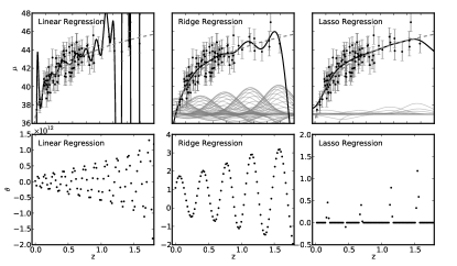
Figure 1 uses Gaussian basis function regression to illustrate how ridge regression constrains the regression coefficients for simulated supernova data. We fit $\mu$, a measure of the distance based on brightness, vs $z$, a measure of the distance based on the expansion of space. The form of this relationship can yield insight into the geometry and dynamics of the expanding universe: similar observations led to the discovery of dark energy [3, 4]. The left panel of Figure 1 shows a general linear regression using 100 evenly spaced Gaussians as basis functions. This large number of model parameters results in an overfitting of the data, which is particularly evident at either end of the interval where data is sparsely sampled. This overfitting is reflected in the lower panel of Figure 1: the regression coefficients for this fit are on the order of 10⁸. The central panel demonstrates how ridge regression (with $\lambda=0.005$) suppresses the amplitudes of the regression coefficients and the resulting fluctuations in the modeled response.

A modification of ridge regression is to use the $L_{1}$-norm to impose sparsity in the model as well as apply shrinkage. This technique is known as Lasso (least absolute shrinkage and selection [5]). Lasso penalizes the likelihood as,

$$\chi^{2}(\boldsymbol{\theta})=(Y-\boldsymbol{\theta}M)^{T}(Y-\boldsymbol{\theta}M)-\lambda|\boldsymbol{\theta}|,$$ (7)

where $|\boldsymbol{\theta}|$ constrains the absolute value of $\boldsymbol{\theta}$. Lasso regularization is equivalent to least squares regression within a constraint on the absolute value of the regression coefficients

$$|\boldsymbol{\theta}|<s.$$ (8)

The most interesting aspect of Lasso is that it not only weights the regression coefficients, it also imposes sparsity on the regression model. This corresponds to setting one (or more if we are working in higher dimensions) of the model attributes to zero. This subsetting of the model attributes reduces the underlying complexity of the model (i.e. we force the model to select a smaller number of features through zeroing of weights). As $\lambda$ increases, the size of the region of parameter space encompassed within the constraint decreases. Figure 1 illustrates this effect for our simulated dataset: of the 100 Gaussians in the input model, with $\lambda=0.005$, only 14 are selected by Lasso (note the regression coefficients in the lower panel). This reduction in model complexity suppresses the overfitting of the data.

In practice, regression applications in astronomy are rarely clean and straight-forward. Heteroscedastic measurement errors and missing or censored data can cause problems. Additionally, the form of the underlying regression model must be carefully chosen such that it can accurately reflect the fundamental nature of the data.

Figure 1: Example of a regularized regression for a simulated supernova dataset $\mu(z)$. We use Gaussian Basis Function regression with a Gaussian of width $\sigma=0.2$ centered at 100 regular intervals between $0\leq z\leq 2$. The lower panels show the best-fit weights as a function of basis function position. The left column shows the results with no regularization: the basis function weights $w$ are on the order of $10^{8}$, and over-fitting is evident. The middle column shows Ridge regression ($L_{2}$ regularization) with $\alpha=0.005$, and the right column shows Lasso regression ($L_{1}$ regularization) with $\alpha=0.005$. All three fits include the bias term (intercept). Dashed lines show the input curve.

III Density Estimation Using Gaussian Mixtures

The inference of the probability density distribution function (pdf) from a sample of data is known as density estimation. Density estimation is one of the most critical components of extracting knowledge from data. For example, given a single pdf we can generate simulated distributions of data and compare against observations. If we can identify regions of low probability within the pdf we have a mechanism for the detection of unusual or anomalous sources.

A common pdf model is the Gaussian mixture model, which describes a pdf by a sum of (often multivariate) Gaussians. The optimization of the model likelihood is typically done using the iterative Expectation-Maximization algorithm [6]. Gaussian mixtures in the presence of data errors are known in astronomy as Extreme Deconvolution (XD) [7]. XD generalizes the EM approach to a case with measurement errors and possible pre-projection of the underlying data. More explicitly, one assumes that the noisy observations $\mathbf{x}_{i}$ and the true values $\mathbf{v}_{i}$ are related through

$$\mathbf{x}_{i}=\mathbf{R}_{i}\mathbf{v}_{i}+\mathbf{\epsilon}_{i}$$ (9)

where $\mathbf{R}_{i}$ is the so-called projection matrix, which may be rank-deficient. The noise $\mathbf{\epsilon}_{i}$ is assumed to be drawn from a Gaussian with zero mean and variance $\mathbf{S}_{i}$. Given the matrices $\mathbf{R}_{i}$ and $\mathbf{S}_{i}$, the aim of XD is to find the model parameters describing the underlying Gaussians and their weights in a way that maximizes the likelihood of the observed data. The EM approach to this problem results in an iterative procedure that converges to (at least) a local maximum of the likelihood. Details of the use of XD, including methods to avoid local maxima in the likelihood surface, can be found in [7].

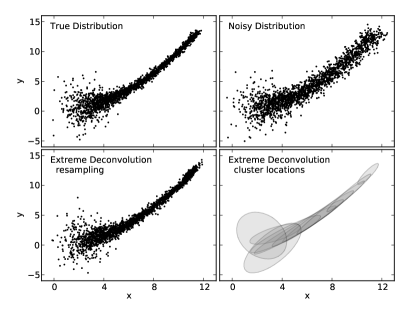
The XD implementation in astroML is used for the example illustrated in Figure 2. The top panels show the true dataset (2000 points) and the dataset with noise added. The bottom panels show the extreme deconvolution results: on the left is a new dataset drawn from the mixture (as expected, it has the same characteristics as the noiseless sample). On the right are the 2-$\sigma$ limits of the ten Gaussians used in the noisy data fit. The important feature of this figure is that from the noisy data, we are able to recover a distribution that closely matches the true underlying data: we have deconvolved the data and the noise.

In practice, one must be careful with XD that the measurement errors used in the algorithm are accurate: If they are over or under-estimated, the resulting density estimate will not reflect that of the underlying distribution. Additionally such EM approaches typically are only guaranteed to converge to a local maximum. Typically, several random initial configurations are used to increase the probability of converging to a global maximum likelihood.

Figure 2: An example of extreme deconvolution showing the density of stars as a function of color from a simulated data set. The top two panels show the distributions for high signal-to-noise and lower signal-to-noise data. The lower panels show the densities derived from the noisy sample using extreme deconvolution; the resulting distribution closely matches that of the high signal-to-noise data.

IV Dimensionality of Data

Many astronomical analyses must address the question of the complexity as well as size of the data set. For example, with imaging surveys such as the LSST [8] and SDSS [9], we could measure arbitrary numbers of properties or features for any source detected on an image (e.g. we could measure a series of progressively higher moments of the distribution of fluxes in the pixels that makeup the source). From the perspective of efficiency we would clearly rather measure only those properties that are directly correlated with the science we want to achieve. In reality we do not know the correct measurement to use or even the optimal set of functions or bases from which to construct these measurements. Dimensionality reduction addresses these issues, allowing one to search for the parameter combinations within a multivariate data set that contain the most information.

Figure 3: A sample of fifteen galaxy spectra selected from the SDSS spectroscopic data set [9]. These spectra span a range of galaxy types, from star-forming to passive galaxies. Each spectrum has been shifted to its rest-frame and covers the wavelength interval 3000–8000 Å. The specific fluxes, $F_{\lambda}(\lambda)$, on the ordinate axes have an arbitrary scaling.

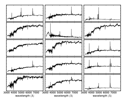
We use SDSS galaxy spectra as an example of high dimensional data. Figure 3 shows a representative sample of these spectra covering the rest-frame wavelength interval 3200–7800 Å in 1000 bins. Classical approaches for identifying the principal dimensions within the large samples of spectroscopic data include: principal component analysis (PCA), independent component analysis (ICA), and non-negative matrix factorization (NMF).

IV-A Principal Component Analysis

PCA is a linear transform, applied to multivariate data, that defines a set of uncorrelated axes (the principal components) ordered by the variance captured by each new axis. It is one of the most widely applied dimensionality reduction techniques used in astrophysics today. Figure 4 shows, from top to bottom, the first four eigenvectors together with the mean spectrum. The first 10 of the 1000 principal components represent 94% of the total variance of the system. From this we can infer that, with little loss of information, we can represent each galaxy spectrum as a linear sum of a small number of eigenvectors. Eigenvectors with large eigenvalues are predominantly low order components (in the context of the astronomical data they reflect the smooth continuum component of the galaxies). Higher order components, which have smaller eigenvalues, are predominantly made up of sharp features such as atomic emission lines, or uncorrelated features like spectral noise.

Figure 4: A comparison of the decomposition of SDSS spectra using PCA (left panel), ICA (middle panel) and NMF (right panel). The rank of the component increases from top to bottom. For the ICA and PCA the first component is the mean spectrum (NMF does not require mean subtraction). All of these techniques isolate a common set of spectral features (identifying features associated with the continuum and line emission). The ordering of the spectral components is technique dependent.

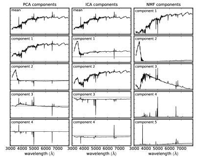
As seen in Figure 4, the eigenspectra of SDSS galaxies are reminiscent of the various stellar components which make up the galaxies. However, one of the often-cited limitations of PCA is that the eigenvectors are based on the variance, which does not necessarily reflect any true physical properties of the data. For this reason, it is useful to explore other linear decomposition schemes.

IV-B Independent Component Analysis

Independent Component Analysis (ICA) [10] is a computational technique that has become popular in the biomedical signal processing community to solve what has often been referred to as blind source-separation or the “cocktail party problem” [11]. In this problem, there are multiple microphones situated through out a room containing $N$ people. Each microphone picks up a linear combination of the $N$ voices. The goal of ICA is to use the concept of statistical independence to isolate (or unmix) the individual signals.

The principal that underlies ICA comes from the observation that the input signals, $s_{i}(\lambda)$, should be statistically independent. Two random variables are considered statistically independent if their joint probability distribution, $f(x,y)$, can be fully described by a combination of their marginalized probabilities, i.e.

$$f(x^{p},y^{q})=f(x^{p})f(y^{q})$$ (10)

where $p$, and $q$ represent arbitrary higher order moments of the probability distributions [12].

ICA refers to a class of related algorithms: in most of these the requirement for statistical independence is expressed in terms of the non-Gaussianity of the probability distributions. The rationale for this is that, by the central limit theorem, the sum of any two independent random variables will always be more Gaussian than either of the individual random variables. This would mean that, for the case of the independent stellar components that make up a galaxy spectrum, the input signals can be approximated by identifying an unmixing matrix, $W$, that maximizes the non-Gaussianity of the resulting distributions. Definitions of non-Gaussianity include the kurtosis of a distribution, the negentropy (the negative of the entropy of a distribution), and mutual information.

The middle panel of Figure 4 shows the ICA components derived via the FastICA algorithm from the spectra represented in Figure 3. As with many multivariate applications, as the size of the mixing matrix grows, computational complexity often makes it impractical to calculate it directly. Reduction in the complexity of the input signals through the use of PCA (either to filter the data or to project the data onto these basis functions) is often applied to ICA applications.

IV-C Non-negative Matrix Factorization

Non-negative matrix factorization (NMF) is similar in spirit to PCA, but adds a positivity constraint on the components that comprise the data matrix $X$ [13]. It assumes that any data matrix can be factored into two matrices, $W$ and $Y$, such that,

$$X=WY,$$ (11)

where both $W$ and $Y$ are non-negative (i.e. all elements in these matrices are $\geq 0$). $WY$ is, therefore, an approximation of $X$. By minimizing the reconstruction error $||(X-WY)^{2}||$ it is shown in [13] that non-negative bases can be derived using a simple update rule,

$$W_{ki} = W_{ki}\frac{[XY^{T}]_{ki}}{[WYY^{T}]_{ki}},$$ (12)

$$Y_{in} = Y_{in}\frac{[W^{T}X]_{in}}{[W^{T}WY]_{in}},$$ (13)

where $n$, $k$, and $i$ denote the wavelength, spectrum and template indices respectively. This iterative process does not guarantee a local minimum, but random initialization and cross-validation procedures can be used to determine appropriate NMF bases.

The right panel of Figure 4 shows the results of NMF applied to the spectra shown in Figure 3. Comparison of the components derived from PCA, ICA, and NMF in Figure 4 shows that these decompositions each produce a set of basis functions that are broadly similar to the others, including both continuum and line emission features. The ordering of the importance of each component is dependent on the technique: in the case of ICA, finding a subset of ICA components is not the same as finding all ICA components [14]. The a priori assumption of the number of underlying components will affect the form of these components.

These types of dimensionality techniques can be useful for identifying classes of objects, for detecting rare or outlying objects, and for constructing compact representations of the distribution of observed objects. One potential weakness of dimensionality reduction algorithms is that the components are defined statistically, and as such have no guarantee of reflecting true physical aspects of the systems being observed. Because of this, one must be careful when making physical inferences from such results.

V Time Series Analysis

Time series analysis is a branch of applied mathematics developed mostly in the fields signal processing and statistics. Even when limited to astronomical datasets, the diversity of applications is enormous. The most common problems range from detection of variability and periodicity to treatment of non-periodic variability and searches for localized events. The measurement errors can range from as small as one part in 100,000, such as for photometry from the Kepler mission [15], to potential events buried in noise with a signal-to-noise ratio of a few at best, such as in searches for gravitational waves using the Laser Interferometric Gravitational Observatory (LIGO) data [16]. Datasets can include many billions of data points, and sample sizes can be in millions, such as for the LINEAR data set with 20 million light curves, each with a few hundred measurements [17]. The upcoming Gaia and LSST surveys will increase existing datasets by large factors; the Gaia satellite will measure about a billion sources close to 100 times during its five year mission, and the ground-based LSST will obtain about 1000 measurements for about 20 billion sources during its ten years of operations. Scientific utilization of such datasets includes searches for extrasolar planets, tests of stellar astrophysics through studies of variable stars and supernovae explosions, distance determination, and fundamental physics such as tests of general relativity with radio pulsars, cosmological studies with supernovae and searches for gravitational wave events.

One of the most popular tools for analysis of regularly (evenly) sampled time series is the discrete Fourier transform. However, it cannot be used when data are unevenly (irregularly) sampled. The Lomb-Scargle periodogram [18, 19, 20] is a standard method to search for periodicity in unevenly sampled time series data. The Lomb-Scargle periodogram corresponds to a single sinusoid model,

$$y(t)=a\,\sin(\omega t)+b\,\cos(\omega t),$$ (14)

where $t$ is time and $\omega$ is angular frequency ($=2\pi f$). The model is linear with respect to coefficients $a$ and $b$, and non-linear only with respect to frequency $\omega$. A Lomb-Scargle periodogram measures the power $P_{LS}(\omega)$, which is a straightforward trigonometric calculation involving the times, amplitudes, and uncertainties of the observed quantity (details can be found in, e.g. [21]). An important property of this technique is that the periodogram $P_{LS}(\omega)$ is directly related to the $\chi^{2}$ of this model evaluated with maximum a-posteriori estimates for $a$ and $b$ [21, 22]. It can be thought of as an “inverted” plot of the $\chi^{2}(\omega)$ normalized by the “no-variation” $\chi^{2}_{0}$ ($0\leq P_{LS}(\omega)<1$).

There is an important practical deficiency in the original Lomb-Scargle method: it is implicitly assumed that the mean value of data values $\overline{y}$ is a good estimator of the mean of $y(t)$. In practice, the data often do not sample all the phases equally, the dataset may be small, or it may not extend over the whole duration of a cycle; the resulting error in mean can cause problems such as aliasing [22]. A simple remedy proposed in [22] is to add a constant offset term to the model from eqn. 14. Zechmeister and Kürster [21] have derived an analytic treatment of this approach, dubbed the “generalized” Lomb-Scargle periodogram (it may be confusing that the same terminology was used by Bretthorst for a very different model [23]). The resulting expressions have a similar structure to the equations corresponding to standard Lomb-Scargle approach listed above and are not reproduced here.

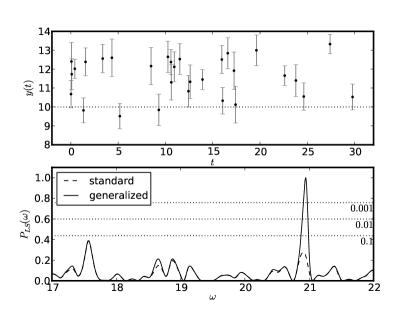
Both the original and generalized Lomb-Scargle methods are implemented in astroML. Figure 5 compares the two in a worst-case scenario where the data sampling is such that the standard method grossly overestimates the mean. While the standard approach fails to detect the periodicity due to the unlucky data sampling, the generalized Lomb-Scargle approach recovers the expected period of $\sim$0.3 days, corresponding to $\omega\approx 21$. Though this example is quite contrived, it is not entirely artificial: in practice this situation could arise if the period of the observed object were on the order of 1 day, such that minima occur only in daylight hours during the period of observation.

The underlying model of the Lomb-Scargle periodogram is non-linear in frequency and thus in practice the maximum of the periodogram is found by grid search. The searched frequency range can be bounded by $\omega_{min}=2\pi/T_{data}$, where $T_{data}=t_{max}-t_{min}$ is the interval sampled by the data, and by $\omega_{max}$. As a good choice for the maximum search frequency, a pseudo-Nyquist frequency $\omega_{max}=\pi\overline{1/\Delta t}$, where $\overline{1/\Delta t}$ is the median of the inverse time interval between data points, was proposed by [24] (in case of even sampling, $\omega_{max}$ is equal to the Nyquist frequency). In practice, this choice may be a gross underestimate because unevenly sampled data can detect periodicity with frequencies even higher than $2\pi/(\Delta t)_{min}$ [25]. An appropriate choice of $\omega_{max}$ thus depends on sampling (the phase coverage at a given frequency is the relevant quantity) and needs to be carefully chosen: a very conservative limit on maximum detectable frequency is of course given by the time interval over which individual measurements are performed, such as imaging exposure time.

An additional pitfall of the Lomb-Scargle algorithm is that the classic algorithm only fits a single harmonic to the data. For more complicated periodic data such as that of a double-eclipsing binary stellar system, this single-component fit may lead to an alias of the true period.

Figure 5: A comparison of standard and generalized Lomb-Scargle periodograms for a signal $y(t)=10+\sin(2\pi t/P)$ with $P=0.3$, corresponding to $\omega_{0}\approx 21$. This example is in some sense a worst-case scenario for the standard Lomb-Scargle algorithm because there are no sampled points during the times when $y_{true}<10$, which leads to a gross overestimation of the mean. The bottom panel shows the Lomb-Scargle and generalized Lomb-Scargle periodograms for these data: the generalized method recovers the expected peak, while the standard method misses the true peak and choose a spurious peak at $\omega\approx 17.6$.

VI Hierarchical Clustering: Minimum Spanning Tree

Clustering is an approach to data analysis which seeks to discover groups of similar points in parameter space. Many clustering algorithms have been developed; here we briefly explore a hierarchical clustering model which finds clusters at all scales. Hierarchical clustering can be approached as a divisive (top-down) procedure, where the data is progressively sub-divided, or as an agglomerative (bottom-up) procedure, where clusters are built by progressively merging nearest pairs. In the example below, we will use the agglomerative approach.

We begin at the smallest scale with $N$ clusters, each consisting of a single point. At each step in the clustering process we merge the “nearest” pair of clusters: this leaves $N-1$ clusters remaining. This is repeated $N$ times so that a single cluster remains, encompassing the entire data set. Notice that if two points are in the same cluster at level $m$, they remain together at all subsequent levels: this is the sense in which the clustering is hierarchical. This approach is similar to “friends-of-friends” approaches often used in the analysis of $N$-body simulations [26, 27]. A tree-based visualization of a hierarchical clustering model is called a dendrogram.

At each step in the clustering process we merge the “nearest” pair of clusters. Options for defining the distance between two clusters, $C_{k}$ and $C_{k^{\prime}}$, include:

$$d_{\rm{min}}(C_{k},C_{k^{\prime}}) = \min_{x\in C_{k},x^{\prime}\in C_{k^{\prime}}}||x-x^{\prime}||$$ (15)

$$d_{\rm{max}}(C_{k},C_{k^{\prime}}) = \max_{x\in C_{k},x^{\prime}\in C_{k^{\prime}}}||x-x^{\prime}||$$ (16)

$$d_{\rm{avg}}(C_{k},C_{k^{\prime}}) = \frac{1}{N_{k}N_{k^{\prime}}}\sum_{x\in C_{k}}\sum_{x^{\prime}\in C_{k^{\prime}}}||x-x^{\prime}||$$ (17)

$$d_{\rm{cen}}(C_{k},C_{k^{\prime}}) = ||\mu_{k}-\mu_{k^{\prime}}||$$ (18)

where $x$ and $x^{\prime}$ are the points in cluster $C_{k}$ and $C_{k^{\prime}}$ respectively, $N_{k}$ and $N_{k^{\prime}}$ are the number of points in each cluster and $\mu_{k}$ the centroid of the clusters.

Figure 6: Dendrogram of a minimum spanning tree over the 2D projection of the SDSS Great Wall. Each of the 8014 points represents the two-dimensional spatial location of a galaxy.

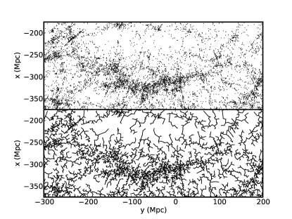
Using the distance $d_{\rm{min}}$ results in a hierarchical clustering known as a minimum spanning tree (see [28, 29, 30], for some astronomical applications) and will commonly produce clusters with extended chains of points. Using $d_{\rm{max}}$ tends to produce hierarchical clustering with compact clusters. The other two distance examples have behavior somewhere between these two extremes.

Figure 6 shows a dendrogram for a hierarchical clustering model using a minimum spanning tree. The data is the SDSS “Great Wall”, a filament of galaxies that is over 100 Mpc in extent [31]. The extended chains of points trace the large scale structure present within the data. Individual clusters can be isolated by sorting the edges by increasing length, then removing edges longer than some threshold. The clusters consist of the remaining connected groups.

Unfortunately a minimum spanning tree is $O(N^{3})$ to compute using a brute-force approach, though this can be improved using well-known graph traversal algorithms. astroML implements a fast approximate minimum spanning tree based on sparse graph representation of links among nearest neighbors, using scipy’s sparse graph submodule.

VII Discussion

The above examples are just a small subset of the analysis methods covered in the astroML codebase. Each of these methods has advantages and disadvantages in practice. A full discussion of these characteristics is beyond the scope of this work; we suggest a careful reading of the references both in this paper and in the astroML code.

To some extent, astroML, and the upcoming companion book, are analogous to the well-known Numerical Recipes book, but aimed at the analysis of massive astronomical data sets with emphasis on modern tools for data mining and machine learning. A strength of astroML lies in the fact that the python code used to download, process, analyze, and plot the data is all open-source and freely available, and that the examples are geared toward common applications in the field of astronomy.

Rather than creating a heavy-weight comprehensive package which duplicates many tools already available in well-known open-source python libraries, astroML places a priority on maintaining a light-weight codebase and using existing tools and packages when available. Notably, code developed for use in astroML has already been submitted upstream, and is included in the latest releases of scipy and scikit-learn, where it is being used by researchers in fields beyond astronomy and astrophysics (notable examples are the BallTree in scikit-learn, and the sparse graph module in scipy). This open-source model of code sharing and development is an increasingly important component of reproducibility of results in the age of data-driven science. We invite all colleagues who are currently developing software for analysis of massive survey data to contribute to the astroML code base. With this sort of participation, we hope for astroML to become a community-driven resource for research and education in data-intensive science.

References

- [1] F. Pedregosa, G. Varoquaux, A. Gramfort, V. Michel, B. Thirion, O. Grisel, M. Blondel, P. Prettenhofer, R. Weiss, V. Dubourg, J. Vanderplas, A. Passos, D. Cournapeau, M. Brucher, M. Perrot, and E. Duchesnay, “Scikit-learn: Machine Learning in Python ,” Journal of Machine Learning Research, vol. 12, pp. 2825–2830, 2011.
- [2] A. N. Tikhonov, Numerical methods for the solution of ill-posed problems, ser. Mathematics and its applications. pub-KLUWER:adr: Kluwer Academic Publishers, 1995, vol. 328.
- [3] A. G. Riess, A. V. Filippenko, P. Challis, A. Clocchiatti, A. Diercks, P. M. Garnavich, R. L. Gilliland, C. J. Hogan, S. Jha, R. P. Kirshner, B. Leibundgut, M. M. Phillips, D. Reiss, B. P. Schmidt, R. A. Schommer, R. C. Smith, J. Spyromilio, C. Stubbs, N. B. Suntzeff, and J. Tonry, “Observational Evidence from Supernovae for an Accelerating Universe and a Cosmological Constant,” AJ, vol. 116, pp. 1009–1038, Sep. 1998.
- [4] S. Perlmutter, G. Aldering, G. Goldhaber, R. A. Knop, P. Nugent, P. G. Castro, S. Deustua, S. Fabbro, A. Goobar, D. E. Groom, I. M. Hook, A. G. Kim, M. Y. Kim, J. C. Lee, N. J. Nunes, R. Pain, C. R. Pennypacker, R. Quimby, C. Lidman, R. S. Ellis, M. Irwin, R. G. McMahon, P. Ruiz-Lapuente, N. Walton, B. Schaefer, B. J. Boyle, A. V. Filippenko, T. Matheson, A. S. Fruchter, N. Panagia, H. J. M. Newberg, W. J. Couch, and Supernova Cosmology Project, “Measurements of Omega and Lambda from 42 High-Redshift Supernovae,” ApJ, vol. 517, pp. 565–586, Jun. 1999.
- [5] R. J. Tibshirani, “Regression shrinkage and selection via the lasso,” Journal of the Royal Statistical Society, Series B, vol. 58, no. 1, pp. 267–288, 1996.
- [6] A. P. Dempster, N. M. Laird, and D. Rubin, “Maximum-likelihood from incomplete data via the em algorithm,” J. R. Stat. Soc. Ser. B, vol. 39, pp. 1–38, 1977.
- [7] J. Bovy, D. Hogg, and S. Roweis, “Extreme deconvolution: Inferring complete distribution functions from noisy, heterogeneous and incomplete observations,” The Annals of Applied Statistics, vol. 5, no. 2B, pp. 1657–1677, 2011.
- [8] Ž. Ivezić, J. A. Tyson, E. Acosta et al., “LSST: from Science Drivers to Reference Design and Anticipated Data Products,” arXiv:0805.2366, May 2008.
- [9] D. G. York, J. Adelman, J. E. Anderson, Jr. et al., “The Sloan Digital Sky Survey: Technical Summary,” AJ, vol. 120, pp. 1579–1587, Sep. 2000.
- [10] P. Comon, “Independent component analysis — a new concept?” Signal Processing, vol. 36, no. 3, pp. 287–314, 1994.
- [11] E. C. Cherry, “Some Experiments on the Recognition of Speech, with One and with Two Ears,” Acoustical Society of America Journal, vol. 25, p. 975, 1953.
- [12] J. V. Stone and J. Porrill, “Independent components analysis for step-wise separation of signals,” Dec. 16 1997.
- [13] D. D. Lee and H. S. Seung, “Algorithms for non-negative matrix factorization,” in Advances in Neural Information Processing Systems 13: Proceedings of the 2000 Conference, T. K. Leen, T. G. Dietterich, and V. Tresp, Eds. Cambridge, Massachusetts: MIT Press, 2001, pp. 556–562. [Online]. Available: http://hebb.mit.edu/people/seung/papers/nmfconverge.pdf
- [14] M. Girolami and C. Fyfe, “Negentropy and kurtosis as projection pursuit indices provide generalised ica algorithms,” 1997.
- [15] D. G. Koch, W. J. Borucki, G. Basri et al., “Kepler Mission Design, Realized Photometric Performance, and Early Science,” ApJL, vol. 713, pp. L79–L86, Apr. 2010.
- [16] B. P. Abbott, R. Abbott, R. Adhikari et al., “LIGO: the Laser Interferometer Gravitational-Wave Observatory,” Reports on Progress in Physics, vol. 72, no. 7, p. 076901, Jul. 2009.
- [17] B. Sesar, J. S. Stuart, Ž. Ivezić, D. P. Morgan, A. C. Becker, and P. Woźniak, “Exploring the Variable Sky with LINEAR. I. Photometric Recalibration with the Sloan Digital Sky Survey,” AJ, vol. 142, p. 190, Dec. 2011.
- [18] E. W. Gottlieb, E. L. Wright, and W. Liller, “Optical studies of UHURU sources. XI. A probable period for Scorpius X-1 = V818 Scorpii.” ApJL, vol. 195, pp. L33–L35, Jan. 1975.
- [19] N. R. Lomb, “Least-squares frequency analysis of unequally spaced data,” Ap&SS, vol. 39, pp. 447–462, Feb. 1976.
- [20] J. D. Scargle, “Studies in astronomical time series analysis. II - Statistical aspects of spectral analysis of unevenly spaced data,” ApJ, vol. 263, pp. 835–853, Dec. 1982.
- [21] M. Zechmeister and M. Kürster, “The generalised Lomb-Scargle periodogram. A new formalism for the floating-mean and Keplerian periodograms,” A&A, vol. 496, pp. 577–584, Mar. 2009.
- [22] A. Cumming, G. W. Marcy, and R. P. Butler, “The Lick Planet Search: Detectability and Mass Thresholds,” ApJ, vol. 526, pp. 890–915, Dec. 1999.
- [23] G. L. Bretthorst, “Generalizing the Lomb-Scargle periodogram-the nonsinusoidal case,” in Bayesian Inference and Maximum Entropy Methods in Science and Engineering, ser. American Institute of Physics Conference Series, A. Mohammad-Djafari, Ed., vol. 568, May 2001, pp. 246–251.
- [24] J. Debosscher, L. M. Sarro, C. Aerts, J. Cuypers, B. Vandenbussche, R. Garrido, and E. Solano, “Automated supervised classification of variable stars. I. Methodology,” A&A, vol. 475, pp. 1159–1183, Dec. 2007.
- [25] L. Eyer and P. Bartholdi, “Variable stars: Which Nyquist frequency?” A&AS, vol. 135, pp. 1–3, Feb. 1999.
- [26] M. Davis, G. Efstathiou, C. S. Frenk, and S. D. M. White, “The evolution of large-scale structure in a universe dominated by cold dark matter,” ApJ, vol. 292, pp. 371–394, May 1985.
- [27] E. Audit, R. Teyssier, and J.-M. Alimi, “Non-linear dynamics and mass function of cosmic structures. II. Numerical results,” A&A, vol. 333, pp. 779–789, May 1998.
- [28] J. D. Barrow, S. P. Bhavsar, and D. H. Sonoda, “Minimal spanning trees, filaments and galaxy clustering,” MNRAS, vol. 216, pp. 17–35, Sep. 1985.
- [29] L. G. Krzewina and W. C. Saslaw, “Minimal spanning tree statistics for the analysis of large-scale structure,” MNRAS, vol. 278, pp. 869–876, Feb. 1996.
- [30] R. J. Allison, S. P. Goodwin, R. J. Parker, S. F. Portegies Zwart, R. de Grijs, and M. B. N. Kouwenhoven, “Using the minimum spanning tree to trace mass segregation,” MNRAS, vol. 395, pp. 1449–1454, May 2009.
- [31] J. R. Gott, III, M. Jurić, D. Schlegel, F. Hoyle, M. Vogeley, M. Tegmark, N. Bahcall, and J. Brinkmann, “A Map of the Universe,” ApJ, vol. 624, pp. 463–484, May 2005.