WITS-CTP-154

In the low temperature confining phase of QCD or QCD-like theories it is challenging to capture the temperature dependence of observables through AdS/CFT. Using the blackfold approach we compute the quark–anti-quark linear static potential in the low temperature confining phase, taking into account the thermal excitations of the string. We find the explicit temperature dependence of the string tension and notice that, as naturally expected, tension decreases as temperature increases. We have also generalized the blackfold approach for the computation of the Wilson loops, making it directly applicable to a large class of backgrounds.

1 Introduction

The static potential between a heavy quark and anti-quark pair, generated by a thin gluonic flux-tube formed between the pair, is of fundamental interest. Confining theories at zero temperature are characterized by a linearly increasing potential at large separation distances with the proportionality constant given by the string tension. The linear behavior in the potential comes from the world-sheet of the string while its quantum fluctuations produce the universal subleading Lüscher term. At low temperatures, below the deconfinement transition temperature, string models predict a decrease of the potential – in particular the string tension decreases as temperature increases. For large separation lengths it has been found that the string tension, $\sigma$, goes like $\sigma=\sigma_{0}-cT^{2}$, where $\sigma_{0}$ is the zero temperature string tension, $T$ is the temperature and $c$ is a constant Pisarski:1982cn ; deForcrand:1984cz ; Gao:1989kg . For a certain range of parameters these predictions were confirmed with Monte Carlo lattice data Bakry:2010zt .

In addition to the string tension, the temperature affects other quantitative and qualitative properties of the confined QQ̄ state. For instance, the flux tube profile differs from the zero temperature one. At zero temperature, it has been found using a string model Luscher19811 and confirmed by several lattice calculations Caselle:1995fh , that the width broadens logarithmically as a function of the bound state size. At low temperature this broadening is modified Bakry:2010zt , increasingly, deviating from the zero temperature result as the temperature increases. In fact, when one approaches the deconfinement temperature, the broadening becomes linear Allais:2008bk .

There have been extensive efforts using string theory models and lattice calculations to understand the temperature dependence of the binding dynamics of a heavy QQ̄ pair. In our paper, we extend these investigations using gauge/gravity duality adscft1 ; adscft2 . We calculate the string tension of a heavy bound state in a confining theory at low temperature, taking into account the thermal excitations of the string.

To our knowledge this is the first top-down AdS/CFT computation that captures the temperature dependence of the string tension. The challenge in setting up this computation is that the low temperature solutions of confining backgrounds do not have a black hole horizon. One can increase the temperature but this leads to a Hawking-Page transition and to a deconfined theory with a black hole. This is a first order transition since there is no smooth solution connecting the two phases. Alternatively, there is a simple geometrical reason to explain the absence of a black hole in the low temperature case. Black hole horizons, associated with a temperature, and cigar type geometries, associated with confinement, are generated by two qualitatively compactifications – the former is along the Euclideanised time direction while the latter is space-like . When the time circle shrinks to zero, the spatial circle does not and vice versa. In other words, one either has a black hole horizon or a scale that introduces confinement encoded in the metric. This is a reason that in confining gauge/gravity theories it is difficult to study the temperature dependence of certain observables. A way to overcome this problem was to introduce bottom-up models to phenomenologically study the static potential Andreev:2006ct ; Ghoroku:2005kg ; BoschiFilho:2006pe . In our paper we capture part of the temperature dependence of the bound state quantities holographically using an alternative more natural method, the blackfold approach, where the string world-sheet corresponding to the Wilson loop, is modified by the thermal excitations generated by the finite temperature of the theory.

We find a temperature dependent string tension, $\sigma=\sigma_{0}-cT^{3}/N$ where $N$ is the number of colors in the theory and $c$ is a known constant, depending on the number of QQ̄ pairs of the bound state. The decrease in the string tension is in qualitative agreement with string model predictions and physical expectation. Note that we did not necessarily expect our result to match with the $T^{n}$ scaling of the string tension for the single quark pair found using effective string models given the differences between the two bound states, the techniques used and the physics that they probe, but the results might be complementary. We elaborate further on this in our paper.

The blackfold approach is an effective theory which aims to describe black branes whose worldvolume is not in stationary equilibrium or flat. It is valid in the probe approximation, for small deviations from the flat stationary black branes on scales much longer than the brane thickness Emparan:2009cs ; Emparan:2009at ; Emparan:2011br ; Emparan:2011hg . For our purpose we use blackfolds to capture the thermal excitations of the string world-sheet corresponding to a Wilson loop in a heat bath. The probe black string is placed in a finite temperature background in thermal equilibrium. This method has already been used for Wilson loops in finite temperature $AdS$ space Grignani:2012iw , in Schrödinger space with scaling $z=2$ Armas:2014nea and giant gravitons in $AdS$ Grignani:2013ewa , as well as in other cases, for example Grignani:2010xm ; Niarchos:2012cy .

We find generic equations, obtained from applying the blackfold approach to black string probes dual to a Wilson loop, which can be applied directly to appropriate backgrounds. It is interesting that this generalization is possible, and allows a direct substitution of the metric elements to obtain the energy of the string in particular backgrounds. This happens with several observables that can be expressed in terms of metric elements using the Nambu-Goto action, including the Wilson loop expectation value Kinar:1998vq ; Giataganas:2012zy ; Giataganas:2013lga ; Brandhuber:1999jr .

To calculate the expectation value of the Wilson loop, rather than the Nambu-Goto action Maldacena:1998im , we use the free energy of the probe, which in the zero temperature limit reproduces the Nambu-Goto result. We use $k$ separate, fundamental strings with $1\ll k\ll N$ and $g_{s}^{2}L\gg 1$. The separate $k$ strings should not be confused with $k$-strings. The $k$-strings correspond to Wilson loops in higher symmetric and antisymmetric representations, and in the dual gravity side are represented as $D3$ and $D5$ branes respectively with electric fluxes Gomis:2006sb ; Gomis:2006im ; Yamaguchi:2006tq . In the blackfold approach a more plausible explanation is that we have $k$ separate QQ̄ flux tubes, that do not interact at zero temperature. Increasing the temperature we find the energy of the $k$ separate strings in thermal equilibrium with the background. We observe that the thermal terms in the energy of the strings do depend on the number of strings in a way that can not be factorized as a common factor in the expression. This means that while bringing the separate strings into thermal equilibrium with the background, the strings do interact although this interaction may be indirect. We point out that this interaction is different from the $k$-string bound state computed by the DBI action of the $D3$ or $D5$ branes.

We apply our generic formulas to confining theories. We choose the AdS soliton background Horowitz:1998ha , and we calculate the new linear static potential taking into account thermal fluctuations and we find a decrease in the string tension. Our work opens new directions, especially in determining the temperature dependence qualitatively in observables in confining theories at low temperature. We remark that in the top-down constructions this has not been achieved until now.

Our paper is organized as follows. In section 2 we provide generic techniques for applying the blackfold method to the Wilson loop string world-sheets for any appropriate background. We obtain the free energy and the constraints on the validity of the results in terms of the background metric elements. Having developed the generic formalism we apply it to the confining $AdS$ soliton background in section 3. We compute the string tension and we find it reduced compared to the zero temperature case. We comment on the modified term in the low temperature case as well as in the high temperature one. We conclude our paper by summarizing and discussing our results in section 4.

2 $k$ F-Strings in Blackfold Approach

In this section, which generalizes Grignani:2012iw , we use the blackfold approach to study the orthogonal QQ̄ Wilson loop in a generic background. In the strong coupling regime we use a number of probe strings ($k$ of them) to construct the finite temperature dual of Wilson loops. The general approach we follow below is for a background with metric $g_{\mu\nu}$ where the probe extends in two dimensions for configurations that satisfy the following equilibrium and boundary conditions Emparan:2011hg

$$T^{ab}K_{ab}^{c}=0~{},\quad T^{ab}n_{b}|_{\partial}=0~{},\quad J^{abc}n_{c}|_{\partial}=0~{}.$$ (2.1)

The equilibrium conditions are on the effective stress energy tensor $T^{ab}$ of the probes and the extrinsic curvature $K^{c}_{ab}$. The boundary conditions are projected with the use of the orthogonal covector at the boundary of the space and also include the case of a charged black probe with an effective current $J$.

By considering the equation of state of the effective fluid that lives in its worldvolume, we get the effective stress energy tensor of the fluid depending on the temperature of the theory $T$. However, as we will see below, it is more convenient to express the temperature dependence of the stress energy tensor implicitly in terms of other parameters.

In order to examine the probes, we consider the generic background

$$ds^{2}=g_{00}dt^{2}+g_{ii}d{x^{i}}^{2}+g_{uu}du^{2}+d{\cal X}^{2}$$ (2.2)

in which the probes are placed. The index $i$ is summed over traverse spatial dimensions and $u$ is the radial coordinate. At the boundary of the background, $u_{b}$, the metric elements $g_{ii}$ diverge, so $g_{ii}(u_{b})=\infty$. When the background includes a black hole, its horizon $u_{h}$, is located at a zero of $g_{00}$, so $g_{00}(u_{h})=0$. ${\cal X}$ is the internal space of the theory and in our analysis plays no role since we consider the string localized at a point on ${\cal X}$. In the most generic treatment an extension of the string in the internal space is allowed, but the form of contributions from the external space in the blackfold approach is not expected to change, apart from certain constants. This is because the additional terms in the string energy due to the blackfold approach are generated from the excitations of the string close to the black hole horizon. Moreover, the additional form fluxes of the generic background do not play any role in the following analysis since they do not couple to the string. Only the $B$-field may play a role, and it couples to the string but its contributions also do not expected to modify qualitatively the form of the energy corrections.

To simplify the form of various equations we define the following quantities

$$f_{1}(u):=|g_{00}(u)|g_{11}(u)~{},\quad f_{u}(u):=|g_{00}(u)|g_{uu}(u)~{},\quad f_{1u}(u):=\frac{g_{11}(u)}{g_{uu}(u)}~{},$$ (2.3)

which will be used in the paper.

To examine the Wilson loop, we choose the radial gauge configuration for the world-sheet

$$t=\tau,\quad u=\sigma,\quad x^{1}=x(\sigma)~{},$$ (2.4)

with the conditions at the boundary, $u_{b}$, of the space being

$$x(u_{b})=0~{},\quad x(u_{b})=L~{}.$$ (2.5)

The induced metric, which contains all the background information we need for our analysis, then reads

$$ds^{2}=g_{00}d\tau^{2}+(g_{uu}+x^{\prime 2}g_{11})d\sigma^{2}~{},$$ (2.6)

where $x^{\prime}:=dx/d\sigma$.

The solution of $k$-coincident black string probes in IIB supergravity gives the effective temperature, $T_{loc}$ , string tension, $T_{s}$, and entropy density, $s$, as Emparan:2011hg

$$T_{loc}=\frac{n}{4\pi r_{0}\cosh\alpha}~{},\qquad T_{s}=\frac{nAr_{0}^{n}\cosh\alpha\sinh\alpha}{k}~{},\qquad s=4\pi Ar_{0}^{n+1}\cosh\alpha~{},$$ (2.7)

where $n:=D-p-3$, $p$ is the black probe spacial dimension, $D$ is the total number of the space-time dimensions, $r_{0}$ is a length scale associated with the horizon, $\alpha$ is a dimensionless charge parameter and $A=\frac{\Omega_{n+1}}{16\pi G}$. The energy momentum tensor elements corresponding to energy density and pressure are

$$\epsilon=T_{00}=Ar_{0}^{n}(n+1+n\sinh^{2}\alpha),\quad P=T_{11}=-Ar_{0}^{n}(1+n\sinh^{2}\alpha)~{}.$$ (2.8)

For strings we consider here, $p=1$, so that for ten dimensional supergravity $n=6$. In the blackfold approach the first law of thermodynamics is equivalent to the equations of motion and therefore the free energy can be used as the action principle. In a generic background with a redshift factor $R_{0}$, the free energy for the string probe (keeping the charge $k$ fixed) reads

$${\cal F}=\int dVR_{0}\left(\epsilon-T_{loc}s\right)=A\int dVR_{0}r_{0}^{6}(1+6\sinh^{2}\alpha)~{},$$ (2.9)

where $V$ is the spacial volume of the world-sheet. Using (2.7) to eliminate $Ar_{0}^{6}$ we can also write the free energy as

$${\cal F}=kT_{s}\int dVR_{0}\left(\frac{1+6\sinh^{2}\alpha}{6\cosh\alpha\sinh\alpha}\right)~{}.$$ (2.10)

The redshift factor $R_{0}$ and the local temperature measured from an asymptotic observer in the induced metric (2.6) are

$$T_{loc}=\frac{T}{R_{0}}~{},\qquad R_{0}(\sigma)=\sqrt{|g_{00}|}~{}.$$ (2.11)

Therefore to achieve asymptotic equilibrium of the probe with the background we need to equate the local temperature with the temperature (2.7) obtaining a relation between $\alpha$ and $r_{0}$:

$$r_{0}=\frac{3\sqrt{|g_{00}|}}{2\pi T\cosh\alpha}~{}.$$ (2.12)

Having specified all the quantities appearing in (2.9) we proceed to solve the resulting equations of motion.

2.1 Free Energy of the QQ̄ configuration

In this section we derive the static potential from the blackfold approach for generic supergravity finite temperature backgrounds. Using the definitions (2.3), the form of the induced metric and the equation (2.12), the free energy (2.9) in the radial gauge for the thermal $F$-string probe in a generic background reads

$${\cal F}=A\left(\frac{3}{2\pi T}\right)^{6}\int d\sigma\sqrt{f_{u}(u)}\sqrt{1+f_{1u}(u)x^{\prime 2}}|g_{00}|^{3}\frac{1+6\sinh^{2}\alpha}{\cosh^{6}\alpha}~{}.$$ (2.13)

Varying the free energy with respect to $x(\sigma)$ leads to the equation of motion

$$x^{\prime}=\left(\frac{f_{1u}^{2}G(\sigma)^{2}}{c^{2}}-f_{1u}\right)^{-1/2}~{},$$ (2.14)

where $c$ is an integration constant and $G(\sigma)$ is defined as

$$G(\sigma):=\sqrt{f_{u}}~{}|g_{00}|^{3}\frac{1+6\sinh^{2}\alpha}{\cosh^{6}\alpha}~{}.$$ (2.15)

The constant $c$, can be related to the turning point of the string $x(\sigma_{0})$ (where $x^{\prime}(\sigma_{0})=0$). It is easily seen from (2.14) that

$$c^{2}=f_{1u}(\sigma_{0})G(\sigma_{0})^{2}~{}.$$ (2.16)

Due to symmetry, the turning point of the string configuration is located at $x(\sigma_{0})=L/2$. Therefore, the distance $L$ between the QQ̄ pairs is obtained by (2.14) and is equal to

$$\frac{L}{2}=\int_{\sigma_{b}}^{\sigma_{0}}d\sigma\left(\frac{f_{1u}^{2}(\sigma)G^{2}(\sigma)}{f_{1u}(\sigma_{0})G^{2}(\sigma_{0})}-f_{1u}(\sigma)\right)^{-1/2}~{}.$$ (2.17)

Now using (2.10) and $T_{s}=1/{\left({2\pi l_{s}^{2}}\right)}=\sqrt{\lambda}/{\left({2\pi R^{2}}\right)}$ (with $\lambda$ the t’Hooft parameter and $R$ the $AdS$ radius), it is convenient to write the free energy as

$${\cal F}=\frac{\sqrt{\lambda}k}{\pi R^{2}}\int_{\sigma_{b}}^{\sigma_{0}}d\sigma\sqrt{f_{u}}\sqrt{1+f_{1u}x^{\prime 2}}Y~{},$$ (2.18)

with

$$Y=\tanh\alpha+\frac{1}{6\cosh\alpha\sinh\alpha}~{},$$ (2.19)

and $\sigma_{b}$ is the boundary of the space either at $u\rightarrow\infty$ or $u\rightarrow 0$. To avoid possible sign errors we choose the boundary at $\sigma_{b}=0$ without loss of generality. The results can be easily converted to the case $\sigma_{b}=\infty$ where $\sigma_{b}>\sigma_{0}$.

2.2 Length scales and constraints

The validity of the blackfold approach for Wilson loop computations puts strong constraints on the parameters of the model which subsequently constrain the turning point of the world-sheet and the length $L$ of the string. The thickness of the F-string $r_{c}=r_{0}(\cosh\alpha\sinh\alpha)^{1/6}$ should be smaller than the other basic length scales in the problem. In a generic case with asymptotic $AdS$, we require that $r_{c}$ is much smaller than the $AdS$ radius ie. $r_{c}\ll R$. In most of the cases another scale is introduced in the radial direction – such as a black hole horizon or a natural cut off of the space (coming for example from a spatial compactification and leading to cigar type geometries). For the confining backgrounds a sensible constraint would be that the radial cut off scale $u_{k}$ is larger that the thickness of the F-string $r_{c}\ll u_{k}$.

To compare length scales, we use (2.7) write $r_{c}$ in terms of $R$ as

$$r_{c}={\left({\frac{kT_{s}}{6AR^{6}}}\right)}^{\frac{1}{6}}R:=\frac{3^{7}}{2^{5}}\kappa^{\frac{1}{6}}R~{},$$ (2.20)

where the dimensionless parameter $\kappa$ has been defined as

$$\kappa:=\frac{2^{5}}{3^{7}}\frac{kT_{s}}{AR^{6}}=B(\sigma)\frac{\sinh\alpha}{\cosh^{5}\alpha}~{},\quad\mbox{with}\quad B(\sigma)=\frac{|g_{00}|^{3}}{\pi^{6}T^{6}R^{6}}~{},$$ (2.21)

and the normalization of $\kappa$ is chosen to simplify its relation to $B$ above. From (2.20) we obtain:

$$r_{c}\ll R~{}\Rightarrow\kappa\ll 1~{}.$$ (2.22)

The constant $\kappa$ can also be related to the parameters $\lambda,~{}N$ and $\kappa$ as

$$\kappa=\frac{2^{7}}{3^{6}}~{}\frac{k\sqrt{\lambda}}{N^{2}}~{},$$ (2.23)

where we have used the definition of $A$ given in (2.8) and the fact that $16\pi G_{10}=(2\pi l_{s})^{8}g_{s}^{2}/(2\pi)$, $\lambda=4\pi g_{s}N$ and $\Omega_{7}=\pi^{4}/3$. Notice that by considering the supergravity limit, the condition (2.22) implies that $k\ll N$.

From (2.11) see that as we move into the bulk $T_{loc}$ becomes large as the redshift increases – at some point $T_{loc}$ will become so large that the probe approximation breaks down. For some backgrounds, this constraint, which translates into how deep the worldsheet can extend into the bulk, can be extracted from (2.21). If we assume that, for the background of interest, the redshift factor increases as we go deeper into the bulk and using the fact that $F(\alpha)=\sinh\alpha/\cosh^{5}\alpha$ has a maximal value, one sees that for fixed $\kappa$, (2.21) puts an upper bound on the redshift allowed for the string. Using the maximal value of $F(\alpha)_{max}=16/{\left({25\sqrt{5}}\right)}$ gives the inequality

$$\frac{\kappa}{B(\sigma)}\leq\frac{2^{4}}{25\sqrt{5}}~{}\Rightarrow~{}|g_{00}(u)|^{3}\geq\frac{25\sqrt{5}}{2^{4}}~{}\kappa\pi^{6}R^{6}T^{6}$$ (2.24)

Let $\sigma_{c}$ be the value of $\sigma$ which saturates the inequality (2.24) so that $\sigma\leq\sigma_{c}$ (recall that we take the boundary at $\sigma_{b}=0$).

Another constraint is generated by the requirement that the variation of the local temperature should be small over the length of the string probe:

$$\frac{r_{c}T_{loc}^{\prime}}{T}=-\frac{1}{2}\frac{r_{c}|g_{00}|^{\prime}}{|g_{00}|^{3/2}}\ll 1~{}.$$ (2.25)

This ensures that the string can be regarded as a probe locally in the background.

In general, in order to satisfy the probe approximation limit, especially for the conformal backgrounds, we should keep the turning point of the string relatively far away from the horizon of the black hole of the background. However, in the confining theories these constrains are weaker or even absent.

2.3 Regularized free energy

We eliminate the divergences in the free energy using the usual subtraction of infinite bare quark masses. This translates to subtracting the free energy of two infinite straight strings, ${\cal F}_{\parallel}$, with shape

$$x_{0}=\tau,\quad u=\sigma~{},$$ (2.26)

which gives

$${\cal F}_{\parallel}=\frac{\sqrt{\lambda}k}{\pi R^{2}}\int_{\sigma_{b}}^{\sigma_{c}}d\sigma\sqrt{f_{u}(u)}Y~{},$$ (2.27)

where $\sigma_{c}$ is the critical point saturating (2.24) defined earlier. It follows that the total regularized free energy for a QQ̄ Wilson loop configuration is given by

$${\cal F}_{reg}={\cal F}-{\cal F}_{\parallel}=\frac{\sqrt{\lambda}k}{\pi R^{2}}\left(\int_{\sigma_{b}}^{\sigma_{0}}d\sigma\sqrt{f_{u}(u)}Y\left(\sqrt{1+f_{1u}(u)x^{\prime 2}}-1\right)-\int_{\sigma_{0}}^{\sigma_{c}}d\sigma\sqrt{f_{u}(u)}Y\right)~{},$$ (2.28)

where the $x^{\prime}$ is given by (2.14). To express the free energy in terms of the length, $L$, one should integrate (2.17) and solve for $\sigma_{0}$. The expression $\sigma_{0}{\left({L}\right)}$ can then be inserted into (2.28) to get the static potential in the form $V{\left({L}\right)}$. This procedure is not usually doable analytically without approximations so we find an expansion for the static potential using $\kappa\sim k/N^{2}$ as an expansion parameter.

The last integral of equation (2.28) has $\sigma_{c}$ as a lower limit. However, close to $\sigma_{c}$ the probe approximation for the string in certain backgrounds, might break down. This is usually the case for the conformal backgrounds, while for the confining backgrounds we mostly focus on here, we do not have this problem. For a possible resolution of the issue in the conformal backgrounds, where we can take $\sqrt{f_{u}}\sim 1/\sigma^{2}$, we can write energy from the equation (2.28) as

$${\cal F}_{reg}= \frac{\sqrt{\lambda}k}{\pi R^{2}}\bigg{(}\int_{0}^{\sigma_{0}}d\sigma\sqrt{f_{u}(u)}{\left({Y\left(\sqrt{1+f_{1u}(u)x^{\prime 2}}\right)-1}\right)}-$$ (2.29)

$${\left({\frac{1}{u_{0}}-\frac{1}{u_{c}}+\int_{0}^{\sigma_{c}}d\sigma\sqrt{f_{u}(u)}{\left({1-Y}\right)}}\right)}\bigg{)}~{}.$$

In the limit $\kappa\rightarrow 0$ the last term approaches zero and $\sigma_{c}\rightarrow\sigma_{h}$. Since, in this case the infrared $\sigma_{c}$ dependence is eliminated, we seem to have a sensible regularized energy for the conformal backgrounds. However, although the result is independent of the IR cutoff, special care is needed since, the UV divergence cancellation need to be equivalent to the Legendre transform method Chu:2008xg ; Drukker:1999zq , and the contributions of the infinite strings free energy, ${\cal F}_{\parallel}$, might not be properly taken into account. However, in the confining backgrounds we are mainly interested in, this is not a problem – we will see below that the usual choice for subtraction of the UV divergences is valid.

2.4 Analytic expressions for small $\kappa$ expansion

The equation (2.21) can be written as a quintic in $\cosh^{2}\alpha$:

$$\left(\frac{\kappa}{B}\right)^{2}X^{5}-X+1=0\qquad\mathrm{where}\quad X=\cosh^{2}\alpha~{}.$$ (2.30)

For $(\kappa/B)^{2}<256/3156$, this has two real positive solutions. Taking $\kappa\rightarrow 0$ one of the solutions corresponds to $\alpha\rightarrow 0$ and the other to $\alpha\rightarrow\infty$. The extremal limit of the branes is obtained by sending the local temperature to zero while at the same time $r_{0}\rightarrow 0$ and $\alpha\rightarrow\infty$ keeping the total charge fixed. This means we should take the second root which may be expanded as

$$\begin{split}\alpha&\simeq\mathop{\mathrm{arccosh}}\left(\sqrt{\frac{\sqrt{B(\sigma)}}{\sqrt{\kappa}}-\frac{1}{4}-\frac{5}{32}\frac{\sqrt{\kappa}}{\sqrt{B(\sigma)}}}\right)\\ &\simeq\frac{1}{4}\log\left(\frac{16B(\sigma)}{\kappa}\right)-\frac{3\sqrt{\kappa}}{8\sqrt{B(\sigma)}}+{\cal O}{\left({\frac{\kappa}{B(\sigma)}}\right)}~{}.\end{split}$$ (2.31)

We may now expand the equation of motion (2.14) and subsequently the length $L$ without reference to explicit metric components giving

$$\frac{L}{2}=\int_{0}^{\sigma_{0}}d\sigma\left(l_{0}(\sigma)+\sqrt{\kappa}~{}l_{1}(\sigma)+{\cal O}{\left({\kappa}\right)}\right),{\quad\mbox{where}\quad}$$ (2.32)

$$l_{0}(\sigma):=\sqrt{\frac{f_{1}(\sigma_{0})}{f_{1u}(\sigma)(f_{1}(\sigma)-f_{1}(\sigma_{0}))}}~{},\quad\mbox{and}$$ (2.33)

$$l_{1}(\sigma):=l_{0}(\sigma)\frac{R^{3}\pi^{3}T^{3}}{3}\frac{\left(|g_{00}(\sigma_{0})|^{3/2}-|g_{00}(\sigma)|^{3/2}\right)g_{11}(\sigma)}{\left(f_{1}(\sigma)-f_{1}(\sigma_{0})\right)|g_{00}(\sigma_{0})|^{3/2}\sqrt{|g_{00}(\sigma)|}}~{}.$$ (2.34)

When the integrals can be done analytically the inversion of (2.32) may be possible. The free energy can be also expanded in small $\kappa$ giving

$$E=\int_{0}^{\sigma_{0}}d\sigma{\left({E_{1}+\sqrt{\kappa}E_{2}}\right)}-\int_{\sigma_{0}}^{\sigma_{c}}d\sigma{\left({E_{3}+\sqrt{\kappa}E_{4}}\right)}+{\cal O}{\left({\kappa}\right)}~{},$$ (2.35)

where the exact expressions are presented in the Appendix Acknowledgements:. Notice the second term has a further implicit dependence on $\kappa$ due to the upper bound, $\sigma_{c}$, of the integral. For particular confining backgrounds this dependence might be avoided as we explain below.

3 Blackfold approach in confining backgrounds

In this section we apply our results to confining theories. We examine the relevant thermal excitations of the strings and obtain modifications of the static potential related to the way that the string tension is modified. It is known that for large separation, the static potential has the linear term indicating confinement and higher order corrections depending exponentially on $(-L)$, where $L$ is the length Giataganas:2011nz ; Giataganas:2011uy ; Nunez:2009da . We analytically compute the potential of heavy QQ̄ pairs in the blackfold approach, using the confining theory of the a temperature $AdS_{3}$ soliton background. Corrections to the term linear in $L$ indicate a decrease of the string tension. This is naturally expected as we elaborate below.

3.1 Confining Theory in the low Temperature Phase

The thermal soliton $AdS_{3}$ background in the low temperature phase corresponds to a confining theory. The background has the form

$$ds^{2}=\frac{u^{2}}{R^{2}}{\left({-dt^{2}+dx_{1}^{2}+dx_{2}^{2}+f{\left({u}\right)}d\phi^{2}}\right)}+\frac{R^{2}}{u^{2}f{\left({u}\right)}}du^{2}~{},$$ (3.1)

$$f(u)=1-\frac{u_{k}^{4}}{u^{4}}~{}.$$ (3.2)

The submanifold parametrized by the coordinates $u$ and $\phi$ has the topology of a cigar. The tip of the cigar is at $u=u_{k}$ which introduces a new scale. To avoid a singularity at the tip, the following periodicity conditions must hold

$$\phi\sim\phi+2\pi\rho~{},\quad\quad\rho:=\frac{R^{2}}{u_{k}}~{}.$$ (3.3)

The periodicity of the Euclidean time $t$ is associated with the inverse temperature $1/T:=2\pi u_{h}$ and can be freely chosen. While the time circle never shrinks to zero, the circle in the $\phi$ direction shrinks to zero at the tip .

By exchanging the $\phi$ and $t$ circles we obtain a blackhole background with same the asymptotics, corresponding to the deconfined phase:

$$ds^{2}=\frac{u^{2}}{R^{2}}{\left({-f{\left({u}\right)}dt^{2}+dx_{1}^{2}+dx_{2}^{2}+d\phi^{2}}\right)}+\frac{R^{2}}{u^{2}f{\left({u}\right)}}du^{2}~{},$$ (3.4)

$$f(u)=1-\frac{u_{h}^{4}}{u^{4}}~{}.$$ (3.5)

Here the time circle shrinks to zero at the horizon, $u_{h}$, while the $\phi$ circle does not. To avoid a singularity, we enforce a periodicity condition along the time direction similar to (3.3). Conversely for this solution, the $\phi$ circle may have arbitrary periodicity.

By calculating the free energies of these two finite temperature backgrounds, it can be seen that at low temperatures ($T\lesssim 1/2\pi\rho$) the confining background dominates while the deconfined phase dominates at higher temperatures Horowitz:1998ha ; Aharony:2006da .

Our main focus is on the low temperature confined background (3.1) with the Euclidean time direction compactified but we also study the high temperature deconfined phase (3.4).

3.2 Thermal Excitations in the Confining Phase Background

Using the background (3.1), we calculate the separation of the QQ̄ pairs and the regularized free energy from (2.17) and (2.28) respectively. To get analytic expressions we assume that the leading contributions come from the region close to turning point – this is where the string almost totally lies when $u_{0}\rightarrow u_{k}$ Sonnenschein:1999if ; Giataganas:2011nz . We expand (2.17) in $\kappa$ and treat each order separately integrating order by order. As a final step to invert $u_{0}{\left({L}\right)}$ we Taylor expand the result around $u_{k}$, since the string world-sheet position is taken very close the tip.

After some algebra we find the separation of the pairs to be

$$L=\frac{R^{2}}{2u_{k}}{\left({c_{1}-\log\left(\frac{u_{0}}{u_{k}}-1\right)}\right)}+\sqrt{\kappa}\frac{\pi^{3}R^{8}T^{3}}{8u_{k}^{4}}\left(c_{2}+\log\left(\frac{u_{0}}{u_{k}}-1\right)\right)~{},$$ (3.6)

where we have omitted higher order terms of ${\cal O}{\left({k}\right)}$. The values of the constants $c_{1}<0$ and $c_{2}>0$ can be found but play no role in the final result as we show below. Subleading constant terms coming from the boundary have been neglected in (3.6). Notice the appearance of a logarithmic term at both ${\cal O}{\left({\kappa^{0}}\right)}$ and ${\cal O}{\left({\kappa^{1/2}}\right)}$. This hints that higher orders of $\kappa$ contribute to the linear term as well as to the exponential corrections. On top of that the sign difference between the logarithmic terms hints that the contribution will not be additive which we verify below. We remark that the above formula for the dipole distance $L$ is valid only when the length is large.

Solving for $u_{0}$ in (3.6) and expanding in $\kappa$ we obtain

$$u_{0}=u_{k}{\left({1+e^{c_{1}-\frac{2Lu_{k}}{R^{2}}}}\right)}+\sqrt{\kappa}e^{c_{1}-\frac{2Lu_{k}}{R^{2}}}\frac{\pi^{3}R^{4}T^{3}}{4u_{k}^{2}}{\left({{\left({c_{1}+c_{2}}\right)}R^{2}-2Lu_{k}}\right)}~{}.$$ (3.7)

The term of ${\cal O}{\left({\sqrt{\kappa}}\right)}$ in (3.7) has a similar form to the zero-th order term with a sign difference and an additional term of the form $\sim L\exp{\left({-L}\right)}$.

The leading contributions to energy come from the region of the string around $u_{k}$ and are calculated from (2.28). Therefore, we integrate (2.28) focusing on the leading contributions around the turning point of the string close to the tip of the geometry.

After some algebra and taking into account carefully the contributions of the incomplete Elliptic integrals we find

$${\cal F}_{reg}=\frac{\sqrt{\lambda}k}{\pi R^{2}}{\left({\frac{u_{k}}{4}{\left({c_{e1}-\log\left(\frac{u_{0}}{u_{k}}-1\right)}\right)}+\sqrt{\kappa}\frac{\pi^{3}R^{6}T^{3}}{48u_{k}^{2}}{\left({c_{e2}+7\log\left(\frac{u_{0}}{u_{k}}-1\right)}\right)}}\right)}~{},$$ (3.8)

where $c_{e1}<0$ and $c_{e2}>0$ are constants that are determined but have subleading effects. We observe that the order $\kappa^{0}$ and $\kappa^{1/2}$ terms are of the same form albeit with different signs. To express the energy in terms of the distance between the pairs we use (3.7) which gives

$${\cal F}_{reg}=\frac{\sqrt{\lambda}k}{2\pi R^{2}}{\left({C_{1}u_{k}+{\left({\frac{u_{k}}{R}}\right)}^{2}L+\sqrt{\kappa}\frac{\pi^{3}R^{4}T^{3}}{3u_{k}^{2}}\left(C_{2}R^{2}-Lu_{k}\right)}\right)}~{},$$ (3.9)

where $C_{1}$ and $C_{2}$ are constants given by

$$C_{1}=\frac{c_{e1}-c_{1}}{2}~{},\qquad C_{2}=\frac{1}{8}{\left({4c_{1}-3c_{2}+c_{e2}}\right)}~{}.$$ (3.10)

Using the final regularized energy expression we find that the string tension becomes

$${\cal F}_{linear}=\frac{\sqrt{\lambda}k}{2\pi R^{2}}\left({\left({\frac{u_{k}}{R}}\right)}^{2}-\sqrt{\kappa}\frac{\pi^{3}R^{4}T^{3}}{3u_{k}}\right)L~{}.$$ (3.11)

Therefore using the blackfold approach, we find that the string tension of the tube between the heavy quark bound state is decreased as temperature is increased. This is in agreement with the expectations, since a bound state like quarkonium dissociates more easily with increasing temperature.

A comment on the additional term in the tension (3.11) and the results of effective string theory models, is in order. For large strings at finite temperature the string tension has been calculated using effective string models and the Nambu-Goto action. The low temperature expansion of the string tension was found to be Pisarski:1982cn

$$\sigma{\left({T}\right)}=\sigma_{0}-\frac{{\left({d-2}\right)}\pi}{6}T^{2}+\sum_{n\geq 3}a_{n}T^{n}~{},$$ (3.12)

where $\sigma_{0}$ is the string tension in zero temperature. The second term is similar to the Lüscher term of the static potential and does not depend on the gauge group of the theory considered. Considering a version of open string-duality Luscher:2004ib , it was shown that the cubic term is absent since $a_{3}=0$. Here we are bringing $k$-interacting strings to thermal equilibrium with the background and we calculate the string tension of the bound state. Unfortunately taking the limit of the single string is not smooth since the blackfold approach is not valid anymore. Therefore, we can not predict with certainty if a cubic term arises in the single string tension when a string is in thermal equilibrium with the theory.

Moreover, notice that the critical distance obtained by (2.24) is

$$u_{c}^{3}=\frac{5^{5/4}}{4}\pi^{3}\sqrt{\kappa}R^{6}T^{3}$$ (3.13)

which does not impose any strict constraint on the system since is close to the boundary and can always be taken such that is less than the $u_{k}$. Furthermore requiring that the width of the F-string, $r_{c}$ is much smaller $u_{k}$ leads to $\kappa^{\frac{1}{6}}\ll u_{k}/R$ which does not constrain our calculations.

The analytical results obtained in this section are supported below by numerical computations done using the full system of equations .

3.3 Numerical Analysis

In this section we numerically compute the energy of the bound state in terms of the distance between the pairs. We use the full equations of motion, and compute the potential $V{\left({L}\right)}$ without any approximation for several values of $\kappa$ including $\kappa=0$. Then we do a linear fit of the form $V=\sigma_{\kappa}L+c_{\kappa}$, where $\sigma_{\kappa}$ is the string tension and $c_{\kappa}$ is a constant, both depending $\kappa$.

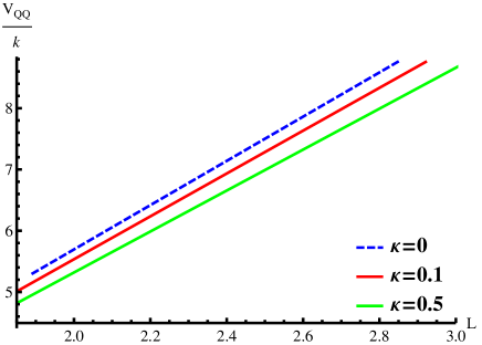
Figure 1: The Energy of the bound state per number of pairs for $\kappa=0,~{}0.1~{},0.5$, with temperature fixed, plotted for large $L$. The value $\kappa=0$ corresponds to the usual Wilson loop Plateau problem with the Nambu-Goto action minimization, while for $\kappa\neq 0$ the blackfold method is applied. Increasing $\kappa$ decreases the slope corresponding to a decrease of the string tension. This is in agreement with the analytical result obtained in (3.9). For the computation we have made the following choices: $R=1,~{}u_{k}=1.9R,~{}T=0.4/R$ . The energy is divided by $\sqrt{\lambda}/{\left({2\pi R^{2}}\right)}$ and the dimensionful quantity $R$ is used to make the $V_{QQ}$ and $L$ dimensionless. For $\kappa=0.1$ and $\kappa=0.5$, the critical distances where our method is valid, are $u_{crit}\simeq 1.05R$ and $u_{crit}\simeq 1.38R$ respectively.

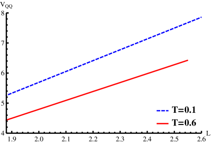
Figure 2: The Energy of the bound state (in units of $R$) for $T=0.1$ and $T=0.6$ with $\kappa$ fixed and plotted for large values of $L$. Increasing the temperature decreases the slope which translates to a decrease of the string tension in agreement with the analytical result (3.9). We have chosen $\kappa=0.2$, and the other parameters and normalizations to be the same as in Figure 2. For $T=0.1$ and $T=0.6$, the critical distances for our method to be valid are $u_{crit}\simeq 0.3R$ and $u_{crit}\simeq 1.78R$ respectively.

We compare the plots and the fitted curves for different values of $\kappa$ and find results supporting the analytic results of the previous section. More specifically, Figure 2 shows the $V_{\kappa}{\left({L}\right)}$ per number of strings $k$, for $\kappa=0,~{}\kappa=0.1$ and $\kappa=0.5$ with $L$ large and temperature fixed. The $\kappa=0$ case corresponds to the Nambu-Goto treatment, while for non-zero $\kappa$ the blackfold terms appear. Increasing $\kappa$ decreases the slope and therefore the string tension per string. The linear fitting leads to

$$\frac{V_{k}{\left({L}\right)}}{k}=\frac{\sqrt{\lambda}}{2\pi R^{2}}{\left({c_{\kappa}+\{3.61,3.50,3.35\}~{}L}\right)}~{},\quad\mbox{for}\quad\kappa=\{0,~{}0.1,~{}0.5\}~{}.$$

where $c_{\kappa}$ is a constant depending on $\kappa$ weakly and the number of strings $k$ is taken equal to 1 for $\kappa=0$. Note that in contrast to the potential per number of strings $V_{k}{\left({L}\right)}/k$, the total potential and the string tension of the whole bound state is increased when the $\kappa$ is increased, since the number of strings $k$ is proportional to $\kappa$ from equation (2.23).

Next we compute the potential of the bound state with a large size $L$ for two different values of the temperature with $\kappa\neq 0$ and fixed, and compare the obtained slopes. The outcome can be seen in Figure 2. The linear fittings of the potential gives

$$V{\left({L}\right)}=\frac{\sqrt{\lambda}k}{2\pi R^{2}}{\left({c{\left({T}\right)}+\{3.60,2.98\}~{}L}\right)}~{},\quad\mbox{for}\quad T=\{0.1,~{}0.6\}~{},$$

where $c{\left({T}\right)}$ depends on $T$. The string tension of the bound state is decreased with increasing temperature as our analytical results indicate (3.11). As mentioned in the previous section, this is expected since the binding of quarkonium becomes weaker at higher temperatures.

3.4 Thermal Excitations in the Non-Confining phase

In the high temperature phase, with background blackhole metric (3.4), the dual gauge theory is no longer confining. The temperature can be found from the periodicity of the Euclidean time circle and is given by $T=u_{h}/{\left({\pi R^{2}}\right)}$.

In this case, Wilson loop calculations can in principle be done analytically. The string configuration needed for the Wilson loop extends along the time, one spatial and the radial direction and is localized along the rest of the directions. Unfortunately, the scale introduced by the black hole leads to stronger constraints on the validity of our method.

Applying our generic equations (2.17) and (2.29) to the background (3.4), we obtain the deconfined results also obtained in Grignani:2012iw

$${\cal F}_{loop}=-\frac{\sqrt{\lambda}k}{L}{\left({\frac{4\pi^{2}}{\Gamma{\left({\frac{1}{4}}\right)}^{4}}+c\frac{\sqrt{k}\lambda^{\frac{1}{4}}}{N}\frac{\Gamma{\left({\frac{1}{4}}\right)}^{4}}{96}{\left({LT}\right)}^{3}+\frac{3\Gamma{\left({\frac{1}{4}}\right)}^{4}}{160}{\left({LT}\right)}^{4}+\dots}\right)}~{}.$$ (3.14)

In the above formula we notice a remarkable similarity with some already known results. The $1/N$ correction happens to be, up to constants, the square root of the energy of the higher representation Wilson loops. For example the circular Wilson loop in the $k$-th symmetric product representation of $U{\left({N}\right)}$, corresponding to a D3 brane, is found to have a term proportional to $k^{3}\lambda^{3/2}/N^{2}$ Drukker:2005kx which is the square of the ${\cal O}{\left({k^{3/2}}\right)}$ term of (3.14). The higher representation Wilson loops can be thought as representing interacting QQ̄ strings of $k$ different pairs, and the interaction term in the energy always appears as a multiple of $1/N^{2}$. In the blackfold approach we have at zero temperature $k$ non-interacting strings, and the nature of this term may be due to some indirect interaction between the strings that is introduced when the string is brought into thermal equilibrium with the background.

4 Conclusions

We have developed a generic formalism applicable to any background (with diagonal metrics), which describes the string world-sheet dual to a Wilson loop using the blackfold approach. Our formulas are in terms of the metric elements. In the energy of the bound state, the thermal excitations of the string due to the finite temperature of the theory have been captured. This is along the same lines as the string Nambu-Goto treatment where several observables, including the energy of the heavy quark bound state, have been expressed in terms of metric elements in generic formulas, applicable to large classes of backgrounds.

We have applied our generic formalism to a confining theory, the AdS soliton, and have found that the string tension is reduced due to the thermal excitations with a negative term proportional to $c\sqrt{\kappa}T^{3}/u_{k}$, where $c$ is a dimensionful constant that has been found. We remark that this is the first time where AdS/CFT top-down techniques have been used to find a temperature dependent observable related to heavy quarks in the confining phase of the theory. To capture the temperature dependence of an observable in a confining theory at low temperature through AdS/CFT is a difficult task, due to the fact that the finite temperature and the confining scale are introduced by a time and space compactification respectively that are competing with each other, and only one circle can shrink to zero at a time. This is why the thermal confining backgrounds, below the Hawking-Page transition have no black hole in their horizon. So the only way one can see the effect of the temperature in an observable is to introduce it in a different way which is what we have done here.

The effect of the temperature on the string tension, we have found, has some interesting features. First of all, this is exactly what is expected to happen qualitatively to the string tension when the heavy bound state starts to heat up. This has been also confirmed by the string motivated models and Monte Carlo lattice computations Pisarski:1982cn ; deForcrand:1984cz ; Gao:1989kg ; Bakry:2010zt . We note that the additional terms depending on the temperature, are not exactly the same as the ones that the string models predict. In retrospect this is not too surprising given differences between the two approaches and the bound states considered. Here we have $k$ number of strings in thermal equilibrium with the background and we calculate the string tension of the bound state, where the limit of the single string is not smooth since there the blackfold approach is not valid anymore. Therefore, we can not predict with certainty that the terms we have found arise also in the expression for the tension of a single string in thermal equilibrium with the background. Moreover, we expect that the appropriately modified methods of the effective string models, should produce analogous terms in the string tension in the context of AdS/CFT, making our approach in a sense complementary to those.

It is essential to point out that we interpret the static potential that we have calculated as coming from a number of QQ̄ pairs in the fundamental representation which we consider to be initially non-interacting at zero temperature. Bringing the strings into thermal equilibrium with the bath affects the energy of the stack of the strings considerably. The terms generated with the blackfold approach depend on the number $k$ of the strings in such a way that it can not be factored out as a common factor. This implies that, even indirectly, there is an interaction between the flux tubes of the different pairs while bringing them into thermal equilibrium. This configuration is different from the bound state of the $k$-strings made by the interaction of the gluonic strings and represented in the gravity dual as $D3$ or $D5$ branes. We nevertheless found a similarity in the mathematical expressions between the $k$-string energy term and the term generated by the blackfold term.

It would be very interesting to study the string tension’s dependence on the temperature in larger class of confining theories and dimensions. This would give information on how the string tension is modified among the different theories in low temperature confining phase. Currently there are limitations of the blackfold approach application to theories with non-constant dilaton and there are not many confining theories where our calculations can be directly extended. Nevertheless, this is an interesting future direction.

Our approach has a wide range of further applications for finding the qualitative properties of observables depending on the temperature in confining theories. Extending our work, it should be possible to take into account the thermal excitation of the strings by applying the blackfold approach and obtain finite temperature effects on other observables.

References

- (1) R. D. Pisarski and O. Alvarez, Strings at Finite Temperature and Deconfinement, Phys.Rev. D26 (1982) 3735.
- (2) P. de Forcrand, G. Schierholz, H. Schneider, and M. Teper, The String and Its Tension in SU(3) Lattice Gauge Theory: Towards Definitive Results, Phys.Lett. B160 (1985) 137.
- (3) M. Gao, Heavy Quark Potential at Finite Temperature From a String Picture, Phys.Rev. D40 (1989) 2708.
- (4) A. Bakry, D. Leinweber, P. Moran, A. Sternbeck, and A. Williams, String effects and the distribution of the glue in mesons at finite temperature, Phys.Rev. D82 (2010) 094503, [arXiv:1004.0782].
- (5) M. Lüscher, G. Münster, and P. Weisz, How thick are chromo-electric flux tubes?, Nuclear Physics B 180 (1981), no. 1 1 – 12.
- (6) M. Caselle, F. Gliozzi, U. Magnea, and S. Vinti, Width of long color flux tubes in lattice gauge systems, Nucl.Phys. B460 (1996) 397–412, [hep-lat/9510019].
- (7) A. Allais and M. Caselle, On the linear increase of the flux tube thickness near the deconfinement transition, JHEP 0901 (2009) 073, [arXiv:0812.0284].
- (8) J. M. Maldacena, The large n limit of superconformal field theories and supergravity, Adv. Theor. Math. Phys. 2 (1998) 231–252, [hep-th/9711200].
- (9) E. Witten, Anti-de sitter space and holography, Adv. Theor. Math. Phys. 2 (1998) 253–291, [hep-th/9802150].
- (10) O. Andreev and V. I. Zakharov, Heavy-quark potentials and AdS/QCD, Phys.Rev. D74 (2006) 025023, [hep-ph/0604204].
- (11) K. Ghoroku and M. Yahiro, Holographic model for mesons at finite temperature, Phys.Rev. D73 (2006) 125010, [hep-ph/0512289].
- (12) H. Boschi-Filho, N. R. Braga, and C. N. Ferreira, Heavy quark potential at finite temperature from gauge/string duality, Phys.Rev. D74 (2006) 086001, [hep-th/0607038].
- (13) R. Emparan, T. Harmark, V. Niarchos, and N. A. Obers, World-Volume Effective Theory for Higher-Dimensional Black Holes, Phys.Rev.Lett. 102 (2009) 191301, [arXiv:0902.0427].
- (14) R. Emparan, T. Harmark, V. Niarchos, and N. A. Obers, Essentials of Blackfold Dynamics, JHEP 1003 (2010) 063, [arXiv:0910.1601].
- (15) R. Emparan, Blackfolds, arXiv:1106.2021.
- (16) R. Emparan, T. Harmark, V. Niarchos, and N. A. Obers, Blackfolds in Supergravity and String Theory, JHEP 1108 (2011) 154, [arXiv:1106.4428].
- (17) G. Grignani, T. Harmark, A. Marini, N. A. Obers, and M. Orselli, Thermal string probes in AdS and finite temperature Wilson loops, JHEP 1206 (2012) 144, [arXiv:1201.4862].
- (18) J. Armas and M. Blau, Black probes of Schrodinger spacetimes, JHEP 1408 (2014) 140, [arXiv:1405.1301].
- (19) G. Grignani, T. Harmark, A. Marini, and M. Orselli, Thermal DBI action for the D3-brane at weak and strong coupling, JHEP 1403 (2014) 114, [arXiv:1311.3834].
- (20) G. Grignani, T. Harmark, A. Marini, N. A. Obers, and M. Orselli, Heating up the BIon, JHEP 1106 (2011) 058, [arXiv:1012.1494].
- (21) V. Niarchos and K. Siampos, Entropy of the self-dual string soliton, JHEP 1207 (2012) 134, [arXiv:1206.2935].
- (22) Y. Kinar, E. Schreiber, and J. Sonnenschein, Q anti-Q potential from strings in curved space-time: Classical results, Nucl.Phys. B566 (2000) 103–125, [hep-th/9811192].
- (23) D. Giataganas, Probing strongly coupled anisotropic plasma, JHEP 1207 (2012) 031, [arXiv:1202.4436].
- (24) D. Giataganas, Observables in Strongly Coupled Anisotropic Theories, PoS Corfu2012 (2013) 122, [arXiv:1306.1404].
- (25) A. Brandhuber and K. Sfetsos, Wilson loops from multicenter and rotating branes, mass gaps and phase structure in gauge theories, Adv.Theor.Math.Phys. 3 (1999) 851–887, [hep-th/9906201].
- (26) J. M. Maldacena, Wilson loops in large N field theories, Phys.Rev.Lett. 80 (1998) 4859–4862, [hep-th/9803002].
- (27) J. Gomis and F. Passerini, Holographic Wilson Loops, JHEP 0608 (2006) 074, [hep-th/0604007].
- (28) J. Gomis and F. Passerini, Wilson Loops as D3-Branes, JHEP 0701 (2007) 097, [hep-th/0612022].
- (29) S. Yamaguchi, Wilson loops of anti-symmetric representation and D5-branes, JHEP 0605 (2006) 037, [hep-th/0603208].
- (30) G. T. Horowitz and R. C. Myers, The AdS / CFT correspondence and a new positive energy conjecture for general relativity, Phys.Rev. D59 (1998) 026005, [hep-th/9808079].
- (31) C.-S. Chu and D. Giataganas, UV-divergences of Wilson Loops for Gauge/Gravity Duality, JHEP 0812 (2008) 103, [arXiv:0810.5729].
- (32) N. Drukker, D. J. Gross, and H. Ooguri, Wilson loops and minimal surfaces, Phys. Rev. D60 (1999) 125006, [hep-th/9904191].
- (33) D. Giataganas and N. Irges, Flavor Corrections in the Static Potential in Holographic QCD, Phys.Rev. D85 (2012) 046001, [arXiv:1104.1623].
- (34) D. Giataganas and N. Irges, Orthogonal Wilson loops in flavor backreacted confining gauge/gravity duality, PoS CORFU2011 (2011) 020.
- (35) C. Nunez, M. Piai, and A. Rago, Wilson Loops in string duals of Walking and Flavored Systems, Phys.Rev. D81 (2010) 086001, [arXiv:0909.0748].
- (36) O. Aharony, J. Sonnenschein, and S. Yankielowicz, A Holographic model of deconfinement and chiral symmetry restoration, Annals Phys. 322 (2007) 1420–1443, [hep-th/0604161].
- (37) J. Sonnenschein, What does the string / gauge correspondence teach us about Wilson loops?, hep-th/0003032.
- (38) M. Luscher and P. Weisz, String excitation energies in SU(N) gauge theories beyond the free-string approximation, JHEP 0407 (2004) 014, [hep-th/0406205].
- (39) N. Drukker and B. Fiol, All-genus calculation of Wilson loops using D-branes, JHEP 0502 (2005) 010, [hep-th/0501109].