Probing the galaxy-halo connection in UltraVISTA to $z\sim 2$

Abstract

We use percent-level precision photometric redshifts in the UltraVISTA-DR1 near-infrared survey to investigate the changing relationship be- tween galaxy stellar mass and the dark matter haloes hosting them to $z\sim 2$. We achieve this by measuring the clustering properties and abundances of a series of volume-limited galaxy samples selected by stellar mass and star-formation activity. We interpret these results in the framework of a phenomenological halo model and numerical simulations. Our measurements span a uniquely large range in stellar mass and redshift and reach below the characteristic stellar mass to $z\sim 2$. Our results are: 1. At fixed redshift and scale, clustering amplitude depends monotonically on sample stellar mass threshold; 2. At fixed angular scale, the projected clustering amplitude decreases with redshift but the co-moving correlation length remains constant; 3. Characteristic halo masses and galaxy bias increase with increasing median stellar mass of the sample; 4. The slope of these relationships is modified in lower mass haloes; 5. Concerning the passive galaxy population, characteristic halo masses are consistent with a simply less-abundant version of the full galaxy sample, but at lower redshifts the fraction of satellite galaxies in the passive population is very different from the full galaxy sample; 6. Finally we find that the ratio between the characteristic halo mass and median stellar mass at each redshift bin reaches a peak at ${\log(M_{h}/M_{\odot})}\sim 12.2$ and the position of this peak remains constant out to $z\sim 2$. The behaviour of the full and passively evolving galaxy samples can be understood qualitatively by considering the slow evolution of the characteristic stellar mass in the redshift range probed by our survey.

Draft Version:

1 Introduction

How are galaxies distributed in dark matter haloes? What is the relationship between visible galaxies and the invisible dark matter? How do the characteristics of these dark matter haloes control the process of galaxy formation? In recent years, considering the dark matter haloes hosting galaxies has provided an alternative perspective on the galaxy formation question by permitting a consideration of how halo mass can regulate star-formation activity.

Although galaxy-galaxy lensing, using the distortion of distant background objects, can measure foreground dark matter mass distributions (Leauthaud et al., 2010), and can provide direct information concerning dark matter halo masses and mass profiles, this technique is challenging observationally and can only probe a relatively narrow redshift baseline as the background galaxy population must be resolved. Even with space-based observations, it is challenging to apply this technique above $z>1$ as foreground galaxies become unresolved.

A simpler although more indirect approach is to compare the observed abundance and clustering properties of the galaxy samples with predictions of phenomenological “halo” models (Scoccimarro et al., 2001; Seljak, 2000; Peacock & Smith, 2000; Neyman & Scott, 1952). These models contain an empirical prescription describing how galaxies populate dark matter haloes (the “halo occupation function”) : their drawback is that they rely on a an accurate knowledge of the halo mass function and halo profile, which must be calibrated using numerical simulations. Although there is some doubt over the applicable regime for these calibrations and the importance of second order effects such as “halo assembly bias” (Croton et al., 2007; Zentner et al., 2014), these techniques remain promising for high-redshift observations where cosmic variances and sample errors are the most important source of uncertainty and systematic errors do not yet dominate. (It is worth mentioning that these assembly bias effects have been shown to be important only in catalogues several orders of magnitudes larger this present work.) A related technique involves comparing the abundances of dark matter haloes with those of high-resolution N-body simulations, the “sub-halo abundance matching” technique (Conroy et al., 2006).

The principal advantage of these methods is that they may be applied over a relatively large redshift baseline and require as observations only abundance and clustering measurements. A considerable industry has developed in recent years (Behroozi et al., 2013; Moster et al., 2010; Conroy & Wechsler, 2009) in applying variants of this model in different redshift ranges and samples and attempting to interpret these results in terms of models of galaxy formation and evolution of star formation activity. However, understanding the derived halo masses and halo occupation functions over large redshift baselines— at least to $z\sim 2$ — has been complicated by the difficulty of comparing diverse data sets with different selection functions. For example, not all samples are cleanly selected in stellar mass and may use either luminosity or even star-formation rate selection (as is the case with colour-colour selected “BzK” (Daddi et al., 2004) galaxies. A final difficulty is that until now most surveys are not deep enough to reach below the all-important characteristic halo mass $M^{*}$ at least to $z\sim 1$, and for this reason have concentrated primarily on more massive galaxies (Foucaud et al., 2010); those that are deep enough have instead been unable to constrain the more massive end because of insufficient area (Bielby et al., 2014). Reaching below this mass limit is important to understand how the rapid build-up of the faint end of the mass function occurs at $z\sim 1$.

The COSMOS field (Scoville et al., 2007) provides a bridge between small, high redshift surveys (like GOODS, CANDELS and other HST deep legacy fields) and larger, intermediate and local surveys like the Canda-France Legacy Survey (Coupon et al., 2012) and the SDSS Zehavi et al. (2011). One of its principal advantages is that it contains a unique collection of spectroscopic redshifts fully sampling $0.5<z<4$ and multi-band photometry Capak et al. (2007) allowing a precise calibration of photometric redshifts, providing a precision better than $1\%$ for both passive and star-forming galaxies. By using broad-band COSMOS data, in combination with the DR1 UltraVISTA near-infrared $YJHK_{\rm~{}s}$ data (McCracken et al., 2012), we are able to accurately determine stellar masses at least until $z\sim 4$ for samples as faint as $K_{\rm s}<24.0$ (Ilbert et al., 2013). Although large local spectroscopic redshift surveys such as BOSS and SDSS have revolutionised our knowledge of the distribution of galaxies in the local Universe, together with more recent magnitude-selected and color-selected surveys such as VIPERS, VVDS and DEEP2 (Davis et al., 2003; Le Fèvre et al., 2005; Guzzo et al., 2014) which allowed measurements to be extended to $z\sim 1$ it is only photometric redshift surveys which can probe the distribution of the galaxy population over such a broad redshift baseline in a single sample to relatively uniform limits. The unique aspect of this current work is our precise stellar mass measurements over a large redshift range.

Previous studies of the halo occupation distribution (the relationship between the number of galaxies in a give dark matter halo and the halo mass) have revealed that the evolution of the angular correlation function and the distribution of satellite galaxies can be adequately explained by an unchanging halo occupation distribution. Some evidence has also emerged that the host halo mass at which the mass in stars reaches a maximum moves slowly towards higher halo masses (Leauthaud et al., 2012; Coupon et al., 2012). In other words, over the lifetime of a halo, star-formation processes occur more efficiently in more massive haloes, and it is tempting to draw a link between this relationship and the observed luminosity-dependant nature of galaxy star-formation rate (Cowie et al., 1996).

Our aim in this work is to use the large, uniform, COSMOS-UltraVISTA photometric redshift catalogue to investigate the relationship between dark matter halo masses and the properties of the visible galaxy population. We will do this by comparing observations (clustering and abundances) of a series of mass-selected galaxy samples to predictions of a theoretical halo model and also to the results of the sub-halo abundance matching using a high-resolution numerical simulation. In this paper we use a flat $\Lambda$CDM cosmology ($\Omega_{\rm m}=0.27$, $\Omega_{\Lambda}=0.73$, $H_{0}=100h\,\textrm{km}\,\textrm{s}^{-1}\,\textrm{Mpc}^{-1}$ and $\sigma_{8}=0.8$) with $h=0.7$. All magnitudes are in the “AB” system (Oke, 1974).

2 The UltraVISTA-COSMOS survey

2.1 Survey overview and photometric redshift estimation

We use the publicly-available UltraVISTA-COSMOS photometric redshift catalogue. This is a near-infrared selected galaxy sample, where objects are detected on a very deep $YJHK_{\rm s}$ “chisquared” (Szalay et al., 1999) detection image: the advantage compared to a simple $K_{\rm s}$ catalogue that is many more bluer sources are included. A complete description of the photometric redshifts derived from this catalogue, and their parent photometric catalogue can be found in Ilbert et al. (2013). The UltraVISTA DR1 release McCracken et al. (2012) covers $1.5~{}\mathrm{deg}^{2}$ of the COSMOS field with deep $YJHK_{\rm s}$ data at least one or two magnitudes deeper than the previous (McCracken et al., 2010) COSMOS near-infrared data.

Photometric redshifts were derived using “Le Phare” (Ilbert et al., 2006; Coupon et al., 2009). “Le Phare” is a standard template fitting procedure using 31 templates including elliptical and spiral galaxies from the Polletta et al. (2007) library and 12 templates of young blue star-forming galaxies from Bruzual & Charlot (2003) stellar population synthesis models. Following standard procedure, the templates are redshifted and integrated through the instrumental transmission curves. The opacity of the intra-galactic medium is accounted for and internal extinction can be added as a free parameter to each galaxy. Photometric redshifts are derived by comparing the modeled fluxes and the observed fluxes with a $\chi^{2}$ merit function. In addition, a probability distribution function is associated to each photometric redshift. A detailed exploration of the precision of these photometric redshifts at intermediate redshifts has been carried out in Ilbert et al. using a unique, large sample of spectroscopic redshifts covering the redshift range $1<z<3$.

We use the usual $\sigma_{\Delta_{z}}/(1+z_{s})$ estimator where $z_{p}$ and $z_{s}$ are the photometric and the spectroscopic redshifts respectively and $\Delta_{z}=z_{p}-z_{s}$. “Catastrophic” redshift errors are defined as objects with $|z_{p}-z_{s}|/(1+z_{s})>0.15$. The percentage of these objects is denoted by $\eta$. Errors were estimated using the normalised median absolute deviation: $1.48\times$ median($|z_{p}-z_{s}|/(1+z_{s})$) (Hoaglin et al., 1983).

For our $K_{\rm s}<24$ cut at $z<1.5$ our photometric redshifts have a precision of better than 1$\%$ and with less than 1$\%$ of catastrophic failures. At $1.5<z<2$, the precision remains excellent at $\sim 0.03$ with the percentage of catastrophic failures less than $\sim 1\%$. Even at $1.5<z<4$, the precision is approximately 3$\%$ with around $7\%$ of catastrophic failures. We limit to our analysis to $z<2.5$: above this redshift range, the number of sources becomes too small to reliably measure clustering or abundances and our cross-bin contamination becomes significant as we will see in Section 3.3, where we investigate the effect of photometric errors on our clustering measurements.

We also use stellar masses computed in Ilbert et al. (2013). The Bruzual & Charlot (2003) stellar population synthesis models with a Chabrier (2003) initial mass function is used to generate a library of synthetic spectra normalised at one solar mass, which are then fitted to the photometric measurements described above using “Le Phare”. As explained in Ilbert et al., “stellar mass” corresponds to the median of the stellar mass probability distribution marginalised over all other parameters. At $z<2$, the uncertainties on the stellar masses are well represented by a Gaussian with $\sigma=0.04*(1+z)$. However, we note that systematic uncertainties can reach 0.1 dex using different templates or as much as 0.2 dex for massive galaxies for two different attenuation curves (see Figure 7 in Ilbert et al. (2010)).

2.2 Sample selection

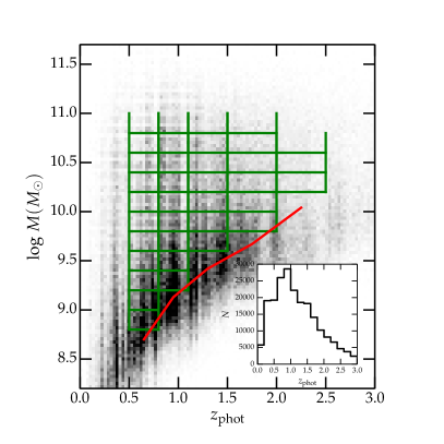
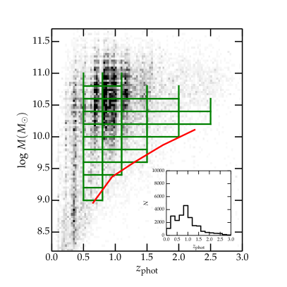
Figure 1: The stellar mass-redshift plane for all UltraVISTA galaxies (left panel) and for passive galaxies (right panel) with $K_{\rm s}<24$. Green lines show our mass thresholds for each sample. The solid red line shows the completeness limits from Ilbert et al. (2013). Inset: the redshift distributions. (Note: the gray-scale for each pixel in the mass-redshift plane is 0–100 objects for the left panel and 0–20 for the right panel.)

We construct a series of volume-limited samples selected by stellar mass. We first select all galaxies with $K_{\rm s}~{}<~{}24$ outside masked regions giving a total of 213,165 objects. After masking, the field has an effective area of 1.5 deg². The mask was constructed from a combined COSMOS $B$, $i$ and $V$ mask together with a mask detailing the borders of the UltraVISTA chi2 image (all stars are masked when one considers the COSMOS masks).

Figure 1 shows the number density of objects as a function of redshift, with the inset panels showing the redshift distribution. The red lines are our mass thresholds and the green ones the completeness limits, as calculated in Ilbert et al. (2013). To calculate this completeness limit, Ilbert et al. computed the lowest stellar mass which could be detected for a galaxy using the relation $\log(M_{\rm limit})=\log(M)+0.4\times(K_{s}-24)$ given a sample at $K_{s}<24$. Then, at a given redshift, the stellar mass completeness limit corresponds to the mass for which $90\%$ of the galaxies have their $M_{\rm limit}$ below the stellar mass completeness limit. The number of objects in each bin, as well as the mean stellar mass, are summarised in Tables 1 and 2. Our large bin widths ($\Delta_{z,min}=0.3$) ensures a low bin-to-bin contamination but still reduces substantially the mixing of physical scales at a given angular scale. Our selected redshift bins are the same as those used in Ilbert et al..

	$0.65<z<0.95$		$0.95<z<1.3$		$1.3<z<1.75$		$1.3<z<1.75$		$1.75<z<2.25$
Threshold(a)	$N_{\rm gal}$	$M_{\rm med}^{(a)}$	$N_{\rm gal}$	$M_{\rm med}^{(a)}$	$N_{\rm gal}$	$M_{\rm med}^{(a)}$	$N_{\rm gal}$	$M_{\rm med}^{(a)}$	$N_{\rm gal}$	$M_{\rm med}^{(a)}$
8.8	26441	9.43	–	–	–	–	–	–	–	–
9.0	21642	9.60	–	–	–	–	–	–	–	–
9.2	17300	9.81	25317	9.84	–	–	–	–	–	–
9.4	13763	10.01	20466	10.02	–	–	–	–	–	–
9.6	10911	10.19	16431	10.21	22666	10.11	–	–	–	–
9.8	8752	10.34	13201	10.36	17361	10.29	16877	10.25	–	–
10.0	7015	10.45	10520	10.50	13280	10.45	12547	10.42	–	–
10.2	5398	10.57	8382	10.61	10000	10.58	9227	10.57	5681	10.58
10.4	3944	10.70	6258	10.74	7242	10.70	6484	10.70	4087	10.71
10.6	2556	10.85	4297	10.85	4828	10.83	4247	10.84	2695	10.83
10.8	1479	11.00	2579	11.00	2698	10.98	2427	10.97	1535	10.98
11.0	742	11.15	1276	11.15	1232	11.14	1094	11.13	–	–

Table 1: Characteristics of each redshift bin for the full $K_{\rm s}<24.0$ galaxy sample. For each stellar mass threshold and redshift bin we report the number of galaxies and the median log stellar mass. ^(a): in $\log(M_{\ast}/M_{\odot})$.

	$0.65<z<0.95$		$0.95<z<1.3$		$1.3<z<1.75$		$1.3<z<1.75$		$1.75<z<2.25$
Threshold(a)	$N_{\rm gal}$	$M_{\rm med}^{(a)}$	$N_{\rm gal}$	$M_{\rm med}^{(a)}$	$N_{\rm gal}$	$M_{\rm med}^{(a)}$	$N_{\rm gal}$	$M_{\rm med}^{(a)}$	$N_{\rm gal}$	$M_{\rm med}^{(a)}$
9.0	3877	10.44	–	–	–	–	–	–	–	–
9.2	3705	10.45	–	–	–	–	–	–	–	–
9.4	3547	10.49	5526	10.59	–	–	–	–	–	–
9.8	3186	10.55	5132	10.64	3560	10.66	–	–	–	–
10.0	2910	10.60	4775	10.67	3342	10.69	1527	10.69	–	–
10.2	2522	10.67	4299	10.73	2998	10.73	1390	10.73	785	10.80
10.4	2041	10.76	3583	10.80	2585	10.79	1182	10.81	714	10.83
10.6	1440	10.88	2717	10.90	2023	10.88	902	10.91	576	10.91
10.8	910	11.04	1803	11.01	1266	11.01	600	11.02	–	–
11.0	498	11.19	939	11.15	–	–	–	–	–	–

Table 2: Characteristics of each redshift bin for the passive $K_{\rm s}<24.0$ galaxy sample. For each stellar mass threshold and redshift bin we report the number of galaxies and the median log stellar mass. ^(a): in $\log(M_{\ast}/M_{\odot})$.

We also considered the quiescent population selected using the criterion $M(NUV)-M(R)>3.5$ defined in Ilbert et al. (2013). After applying object masks, the passive sample is composed of 22,169 objects with, as before, a magnitude cut of $K_{\rm s}<24.0$ . The characteristics of each sample are summarised in Tables 1 and 2. The right panels of Figure 1 show the redshift distribution of this population.

3 Methods

3.1 The angular two-point correlation function

We measure the two-point angular correlation function $w(\theta)$ for our samples using the Landy & Szalay (1993) estimator,

$$w(\theta)=\frac{n_{\rm r}(n_{\rm r}-1)}{n_{\rm d}(n_{\rm d}-1)}\frac{DD}{RR}-\frac{n_{\rm r}-1}{n_{\rm d}}\frac{DR}{RR}+1,$$ (1)

where, for a chosen bin from $\theta$ to $\theta$ + $\delta\theta$, $DD$ is the number of galaxy pairs of the catalog in the bin, $RR$ the number of pairs of a random sample in the same bin, and $DR$ the number of pairs in the bin between the catalog and the random sample. $n_{d}$ and $n_{r}$ are the number of galaxies and random objects respectively. A random catalog is generated for each sample with the same geometry as the data catalog using $n_{\rm r}\sim 400,000$ which is at the most more than 500 and at least 16 times the number of data at each bin. We measure $w$ in each field using a fast two-dimensional tree code in the angular range $0.001<\theta<0.2$ degrees divided into 15 logarithmically spaced bins.

The errors on the two-point correlation measurements are estimated from the data using the jackknife approach (see for example Norberg et al., 2011) using 128 subsamples. Removing one sub-sample at a time, this allows us to compute the covariance matrix as:

$$C(w_{i},w_{j})=\frac{N-1}{N}\sum_{l=1}^{N}(w_{i}^{l}-\overline{w}_{i})(w_{j}^{l}-\overline{w}_{j}),$$ (2)

where $N$ is the total number of subsamples, $\overline{w}$ the mean correlation function and $w^{l}$ the estimate of $w(\theta)$ with the $l$-th subsample removed.

Finally, although one of the largest survey at these redshifts, the UltraVISTA field covers a relatively small area, and as a consequence the integral constraint (see Groth & Peebles, 1977) is expected to have a impact on our clustering measurements leading on an underestimation of the clustering strength by a constant factor $w_{c}$ which can be estimated as follows:

$$w(\theta)=w_{mes}(\theta)+w_{c}.$$ (3)

Assuming that the two-point correlation function is described by a simple power with slope $\gamma$ and amplitude $A$ fitted on the data, it leads to:

$$w_{mes}(\theta)=A\theta^{1-\gamma}-w_{c}\times A(\theta^{1-\gamma}-C).$$ (4)

We can derive $C$ following Roche et al. (1999):

$$C=\frac{\sum\theta^{1-\gamma}RR(\theta)}{\sum RR(\theta)},$$ (5)

and then:

$$w(\theta)=w_{mes}(\theta)\frac{\theta^{1-\gamma}}{\theta^{1-\gamma}-C}.$$ (6)

We find $C\sim 1.42$.

3.2 Halo model implementation and fitting

To connect galaxies to their hosting dark matter haloes, we use a phenomenological “halo” model (for a review see Cooray & Sheth, 2002). In this model, it is assumed that the number of galaxies in a given dark matter halo is a simple monotonic function of the halo mass. By combining this function (the “halo occupation distribution”) with our knowledge of the halo mass function and mass profile, one may predict the abundance and clustering properties of the visible population.

The key underlying assumption is that the number of galaxies $N$ within a halo depends only on the halo mass $M$ and not on environment or formation history: we will address the extent to which these assumptions are reasonable in subsequent sections.

Our model follows closely Zheng et al. (2005) who, motivated by simulations, suggested that the total numbers of galaxies in dark matter halo, $N(M)$ is a sum of two contributions: one from the central galaxy in the halo $N_{c}(M)$ and one coming from the satellites $N_{s}(M)$. Thus $N(M)$ can be expressed as:

$$N(M)=N_{c}(M)\times[1+N_{s}(M)].$$ (7)

We follow Zheng et al. (2007) in which the central galaxy is described as a step function with a smooth transition allowing some scatter in the stellar mass halo mass relation:

$$N_{c}(M)=\frac{1}{2}\Big{[}1+\textrm{erf}\Big{(}\frac{\log M-\log M_{min}}{\sigma_{\log M}}\Big{)}\Big{]},$$ (8)

and a power law with a cut at low halo mass for the satellites:

$$N_{s}(M)=\Big{(}\frac{M-M_{0}}{M_{1}}\Big{)}^{\alpha}.$$ (9)

Our model has five adjustable parameters: $M_{\rm min}$, $M_{1}$, $M_{0}$, $\alpha$ and $\sigma_{\log M}$. In this work, will examine in particular $M_{\rm min}$, which represents the characteristic mass scale for which $50\%$ of haloes host a galaxy, and $M_{1}$, which is the characteristic mass scale for haloes to host one satellite galaxy.

Thus the mean number density of galaxies is given by:

$$n_{\rm{gal}}(z)=\int N(M)n(M,z)dM,$$ (10)

where $n(M,z)$ is the halo mass function for which we use the prescription from Sheth & Tormen (1999).

We use a Navarro-Frenk-White halo density profile (Navarro et al., 1997) and the halo bias parametrisation $b_{h}(M,z)$ from Tinker et al. (2005) which has been calibrated on simulations.

We compute the following derived parameters: the mean halo mass:

$$\langle M_{\rm{halo}}\rangle(z)=\int dMMn(M,z)\frac{N(M)}{n_{\rm gal}(z)},$$ (11)

the mean galaxy bias:

$$b_{\rm{gal}}(z)=\int dMb_{:}{h}(M,z)n(M,z)\frac{N(M)}{n_{\rm{gal}}(z)}$$ (12)

and the satellite fraction:

$$f_{s}(z)=1-f_{c}(z)=1-\int dMn(M,z)\frac{N_{c}(M)}{n_{\rm{gal}}(z)}.$$ (13)

The implementation of the halo model we use is described fully in Coupon et al. (2012).

We derive the best-fitting halo models corresponding to our measurements using the “Population Monte Carlo” (PMC) technique as implemented in the CosmoPMC package to sample likelihood space (Wraith et al., 2009; Kilbinger et al., 2010). For each galaxy sample, we simultaneously fit both the two-point correlation function $w$ and the number density of galaxies $n_{gal}$, by summing both contributions to the total $\chi^{2}$:

$$\chi^{2}=\sum_{i,j}[w^{\rm{obs}}(\theta_{i})-w^{\rm{model}}(\theta_{i})](C^{-1})_{i,j}[w^{\rm{obs}}(\theta_{j})-w^{\rm{model}}(\theta_{j})]$$

$$+\frac{[n^{\rm{obs}}_{\rm{gal}}-n^{\rm{model}}_{\rm{gal}}]^{2}}{\sigma_{\rm{gal}}^{2}},$$ (14)

where $C$ is the data covariance matrix. The error on the galaxy number density $\sigma_{gal}$ contains both Poisson noise and cosmic variance.

3.3 Estimating the effect of photometric redshift errors on clustering measurements

To independently quantify the number of catastrophic photometric redshift outliers, we analyse the spatial cross-correlation of galaxies between different redshift bins. The mis-identification of photo-$z$’s create physical clustering between otherwise un-correlated bins. We use the pairwise analysis introduced in Benjamin et al. (2010) , which considers two redshift bins at a time. With $w_{ij}$ denoting the angular correlation function between redshifts $i$ and $j$, the following combination of cross- and auto-correlation function vanishes for all angular scales $\theta_{t}$,

$$d_{t}=w_{ij}(\theta_{t})\left(f_{ii}f_{jj}+f_{ij}f_{ji}\right)$$

$$-w_{ii}(\theta_{t})\frac{N_{i}}{N_{j}}f_{ij}f_{ji}$$

$$-w_{jj}(\theta_{t})\frac{N_{j}}{N_{i}}f_{ji}f_{ii}.$$ (15)

The number of observed galaxies per bin $i$ is $N_{i}$. The contamination fraction of galaxies originating from the redshift range given by bin $i$, but mis-placed into bin $j$ due to catastrophic failure is denoted with $f_{ij}$. This pairwise approach neglects the contamination from other bins $k\neq i,j$. Therefore, the fraction of galaxies correctly identified in bin $i$ is $f_{ii}=1-f_{ij}$. The approximation of the pairwise analysis is valid for contamination fractions up to 10%.

We restrict our analysis to non-adjacent redshift bins ($|i-j|\leq 1$), since both the large-scale structure and the photo-$z$ dispersion create correlations between galaxies from neighbouring bins that are easily larger than 10%. We follow Coupon et al. and calculate the covariance of the data vector $d_{t}$ using a Jackknife estimate. As in Coupon et al., we neglect the mixed terms in (15), which correlate different correlation functions, since these terms are sub-dominant (Benjamin et al., 2010). The expression for the covariance then becomes

$$C_{ts} =\left\langle d_{t}d_{s}\right\rangle$$

$$=\left\langle w_{ij}(\theta_{t})w_{(}\theta_{s})\right\rangle\left(f_{ii}f_{jj}+f_{ij}f_{ji}\right)^{2}$$

$$+\left\langle w_{ii}(\theta_{t})w_{ii}(\theta_{s})\right\rangle\left(\frac{N_{i}}{N_{j}}f_{ij}f_{ji}\right)^{2}$$

$$+\left\langle w_{ii}(\theta_{t})w_{ii}(\theta_{s})\right\rangle\left(\frac{N_{j}}{N_{i}}f_{ji}f_{ii}\right)^{2}.$$ (16)

We calculate a $\chi^{2}$ null test with $\chi^{2}=\vec{d}_{t}C^{-1}_{st}\vec{d}_{s}$, and fit the two parameters $f_{ij}$ and $f_{ji}$.

As an example, we consider the the galaxy sample with $\log(M_{\ast}/M_{\odot})\sim 10.8$. Here, we find the fraction of catastrophic outliers to be consistent with zero between all pairwise bins (see left panel of Fig. 2 for an example), with the exception of the contamination $f_{13}$ from bin $0.8<z<1.1$ to $1.5<z<2.0$, which is $>3\%$ ($1\sigma$, see right panel of Fig. 2).

The pairwise analysis typically constrains a quadratic combination of the contaminations $f_{ij}$ and $f_{ji}$, and does not provide an independent estimate of the outlier rates. An upper limit of a contamination fraction $f_{ij}$ therefore implies that $f_{ji}$ is zero, or very small. All our upper limits are below $15\%$ ($1\sigma$), with the exception of $f_{41}$ and $f_{42}$, for which the upper limits are $24\%$. The lowest redshift bin $0.5<z<0.8$ is affected the least, with contamination fractions less than $8\%$ from other bins.

To summarise, the cross-correlation analysis independently confirms the very high quality our of photometric redshifts, and is consistent with the low catastrophic outlier rate discussed in Section 2.1.

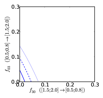
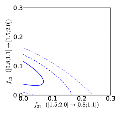
Figure 2: Two examples of constraints contamination fraction $f_{ij}$ obtained from spatial clustering between redshift bin pairs. The solid, dashed, and dotted lines show $1$-, $2$-, and $3$-$\sigma$ contours, respectively. Left panel: Contamination fraction between bins $[0.5;0.8]$ and $[1.5;2]$. Right panel: Contamination fraction between bins $[0.8;1.1]$ and $[1.5;2]$. In both panels, the $x$-($y$-)axis represents the scattering from high to low (low to high) redshifts.

4 Mass-selected clustering measurements

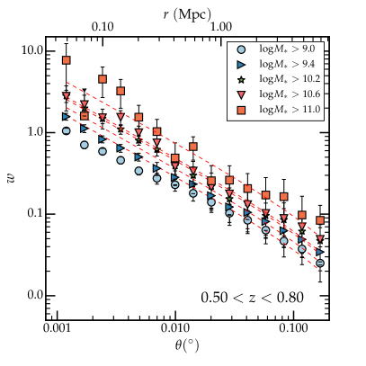
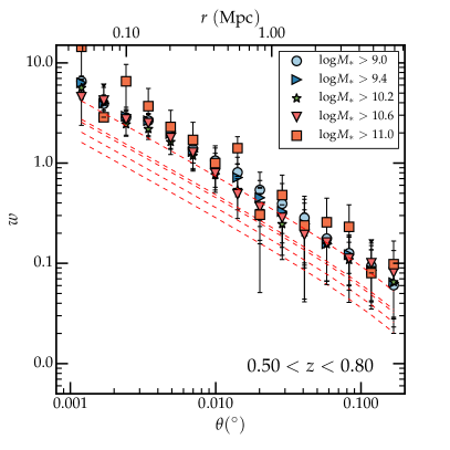
Figure 3: Mass-selected galaxy clustering measurements as a function of angular scale in degrees in the UltraVISTA-COSMOS survey for the full sample (left panel) and the passive galaxy sample (right panel) at $0.5<z<0.8$. The dashed lines correspond to the best-fitting large-scale power laws for the $0.5<z<0.8$ sample (left panel).

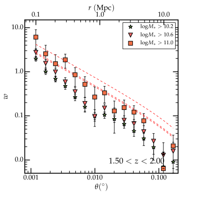
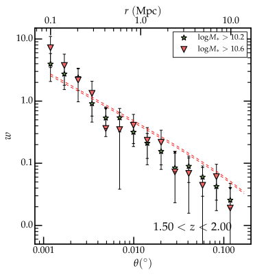
Figure 4: As in Figure 3 but for the $1.5<z<2.0$ bin. The dashed lines show the large-scale fit for the corresponding mass bins in the $0.5<z<0.8$ sample.

We first consider our mass-selected galaxy clustering measurements. In Figures 3 and 4 we show the projected angular correlation function $w$ as a function of angular scale $\theta$ (in degrees) and stellar mass threshold for two representative redshift bins, $0.5<z<0.8$ and $1.5<z<2.0$. The left panels show the full sample, whereas the right panels show the passive galaxy sample. The dotted lines on all panels correspond to the fits on large scales ($\sim 0.1\,{\rm deg}$) to the low-redshift $(0.5<z<0.8)$ full galaxy sample with a fixed slope of $-0.8$. Finally, the top horizontal axes shows the comoving angular separation at the redshift of the sample.

Qualitatively, several trends are immediately apparent. Firstly, at a given stellar mass threshold, for both galaxy types, the clustering amplitude decreases with increasing redshift. Secondly, at a given redshift, the clustering amplitude is higher for samples with higher stellar mass thresholds. Finally, at both redshifts and at the same stellar mass threshold, the clustering amplitude of the passive galaxy population is always higher than the full galaxy population. It is also interesting to note that the dependence of clustering strength on stellar mass threshold is less pronounced for the passive galaxy population at lower redshifts (although this is not the case in other redshift bins not shown here). The explanation of this behaviour is quite straightforward: examining Figure 1, we see that the bulk of the passive population at $z\sim 0.5$ has stellar masses of $10^{10.5}M_{\sun}$: fainter thresholds do not appreciably change the bulk median stellar mass threshold and therefore the overall clustering amplitudes rest unchanged.

Some general comments can also be made concerning the shape of $w$. Firstly, for intermediate stellar mass threshold samples ($M\sim 10^{10}$ $M_{\sun}$) in the lower-redshift $0.5<z<0.8$ bin, $w$ follows closely a power-law with a slope $\gamma\sim 1.8$. However, at higher stellar mass thresholds, the slope of $w$ begins to steepen, whereas at lower stellar mass threshold $M\sim 10^{9}$ $M_{\sun}$ the slope of $w$ is shallower. At high redshifts, finally, the shape of $w$ deviates from a simple power-law: this is seen most clearly if one considers the $M\sim 10^{9.8}$ $M_{\sun}$ at low and high redshifts (filled pentagons in both cases). At high redshifts, a ’break’ is clearly seen at angular scales of $\sim 0.01$ degrees, whereas no such break is visible a lower redshifts.

It is interesting to consider these measurements in the context of previous clustering and mass-selected clustering measurements in the COSMOS field. In an early paper, Meneux et al. (2009) used the zCOSMOS 10k spectroscopic sample to create a series of mass-selected galaxy samples covering $0.2<z<0.5$. Despite the use of spectroscopic redshifts, the comparatively small number of galaxies and the consequently limited dynamic range (only one decade in stellar mass) meant that they were not able to detect clearly the trends outlined here.

Given the complicated nature of the behaviour of $w$ it is clear that fitting a simple power-law (with a corresponding integral constraint correction) misses most of these complex features. In the following Section we will fit our “halo model” to these observed correlation functions and discuss in detail the behaviour of the corresponding derived parameters as a function of both redshift and stellar mass threshold.

5 Halo model analysis

5.1 Fitting the two-point correlation function

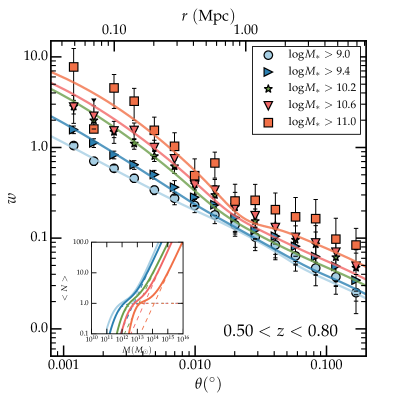
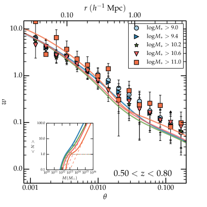
Figure 5: Mass-selected galaxy clustering measurements in the UltraVISTA-COSMOS survey for the full sample (left panel) and the passive galaxy sample (right panel) at $0.5<z<0.8$. The solid lines correspond to the best-fitting halo model for each bin. The inset panel shows the corresponding halo occupation distribution for each of the best-fitting models. Total, satellite and central contributions are shown by the solid, dashed and dot-dashed lines respectively. The top horizontal axis shows the comoving separation corresponding to the angular distance at the effective redshift of the slice.

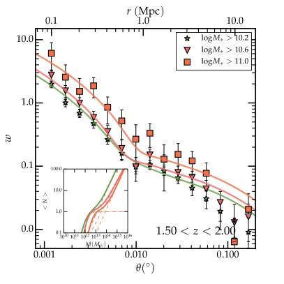
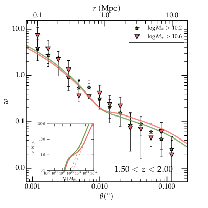
Figure 6: As in Figure 5 but for two samples at $1.5<z<2.0$.

In Figures 5 and 6 the solid lines show the best fitting halo model for a range of stellar mass thresholds for two redshift bins for both passive and total samples. In each Figure, the thick solid line in the inset panel shows the corresponding best-fitting halo occupation distribution for each mass threshold at each redshift. The contribution to the satellite and central term is shown by the dashed and dotted lines respectively. The left and right panels show the measurements for the total and passive sample respectively.

Qualitatively, the fits are good, in particular for the lower-mass threshold bins (note, however, the visual inspection of the fits can be misleading as there is significant co-variance between adjacent bins). In general, lower mass threshold bins are better fit by our halo model. In the following Sections we will consider the derived parameters based on these halo model fits.

It is interesting to compare, at the same redshift, the fits for the passive galaxy population and the full galaxy population. At a comparable mass threshold, the minimum halo masses are higher (inset panel on each figure). In addition, it is interesting to note that the fraction of satellite galaxies is higher for the passive galaxy sample. We will return to this point in later sections.

5.2 Comoving correlation lengths for mass-selected samples

Traditionally, the comoving correlating length, representing the amplitude of the real-space correlation function at 1 Mpc and denoted by $r_{0}$ has been used as a measure of the strength of galaxy clustering. Often, this amplitude has been estimated by fitting a power-law correlation function to the projected correlation function and using it to estimate (sometimes by extrapolation) the correlation function amplitude at $1~{}$Mpc after de-projection using the Limber (1954) formula. This procedure can potentially be problematic: as we have seen, the correlation function is poorly fit by a simple power law, and often the fitted scales lie outside the range of the survey. In this work we adopt a different approach: by using our fitted halo model parameters, we can directly compute $\xi(r)$, the real-space correlation function, at each slice, and from this make a direct measurement of the value of the correlation amplitude at $1~{}$ Mpc. From the top axes of Figures 5 and 6 we note, furthermore, that this $1~{}\mathrm{Mpc}$ scale falls within the survey area at all redshifts.

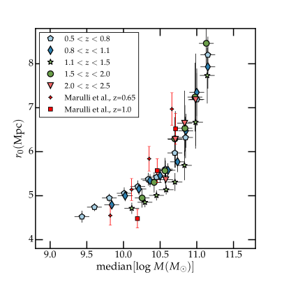
Figure 7: The co-moving correlation length $r_{0}$, in Mpc, computed from our halo model for each redshift slice as a function of stellar mass threshold. The small squares and diamonds show correlation lengths measured in samples thresholded in stellar mass in the VIPERS survey (taken from Table 3 in Marulli et al. 2013).

These fits are plotted in Figure 7 which shows the comoving correlation length $r_{0}$ as a function of sample median stellar mass. Error bars are computed by measuring the standard deviation of $r_{0}$ over a weighted set of 5,000 PMC realisations of our halo model fits. For reference, small symbols show the values derived by Marulli et al. (2013) in VIPERS, and within the error bars, our measurements are in agreement with this work.

We see that the amplitude of the co-moving correlation length increases gradually for samples whose mean stellar masses are smaller than $\log(M_{\ast}/M_{\odot})\sim 11.0$; for samples more massive than this, the amplitude increases steeply. The presence of this “knee” amplitude has been seen previously in lower redshift samples, at least for luminosity-selected samples (see, for example Norberg et al. (2002)). We also we also see that at fixed stellar mass threshold, the clustering amplitude is independent of redshift. Some hints of this behaviour has been seen in previous papers (McCracken et al., 2008; Pollo et al., 2006; Meneux et al., 2009), but this is the first time it has been unambiguously detected over such a large redshift range. Finally, we note that the bin $1.1<z<1.5$ is offset from the others: as we shall see in Section 5.8, this a consequence of the rich structures present at intermediate redshifts in the COSMOS field.

5.3 The characteristic halo mass – galaxy number density relationship

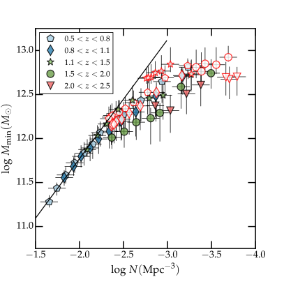
Figure 8: $M_{\rm min}$ as a function of log galaxy number density for each redshift and mass threshold slice (passive galaxy samples are shown by the red open symbols). The solid line corresponds to a fit to the low-mass end of the most abundant samples.

Figure 8 shows $M_{\rm min}$ as a function of galaxy number density (defined in Equation (10) for the full and the quiescent samples (open red symbols respectively). In general, rarer, less abundant objects reside in more massive haloes. Comparing the quiescent population with the full galaxy sample, we see that (within the error bars) for a given galaxy abundance both the quiescent and full galaxy populations lie within haloes of the same dark matter haloes masses (with the exception of the $1.1<z<1.5$ bin, to which we will return to later; this bin is systematically different from all the others). In other words, in the halo mass / stellar mass plane, nothing distinguishes the passive population from the full galaxy population.

The solid line shows a power-law fitted on the five most abundant bins of the lowest-redshift sample $0.5<z<0.8$. It is clear that even for a given redshift slice, a simple power-law fit does not adequately describe the data. Both the $0.5<z<0.8$ and $0.8<z<1.1$ redshift bins, which have sufficient depth to cover a large range in abundances show an inflection point at $\mathrm{log}\sim-2.5$. Higher-redshift bins do not have sufficient depth to reach below this inflection point, so we cannot say definitively if this feature is also present in the higher-redshift data. Concerning redshift evolution of this relation, although our volume-limited samples cover different mass ranges at different redshifts, there is some tentative evidence that at fixed abundances, minimum halo masses required to host galaxies are progressively lower at higher redshifts (the points at $1.5<z<2.0$, for example, are below all the low-redshift points, and this trend continues to even higher redshifts).

Some previous authors have also considered this relationship. Coupon et al., in the CFHTLS, found no evidence for an inflection point in the $M_{\rm min}$ versus $n_{\rm gal}$ relationship between $z=0.2$ and $z=1.2$. However, it should be noted that their samples were only approximately mass-limited; our slope in Figure 8 is steeper than they found. In later Sections we will discuss how this change in slope is related to the evolution of the global stellar mass function, and how the origin of the inflection point is connected to the

5.4 Characteristic halo mass scales as a function of stellar mass and redshift

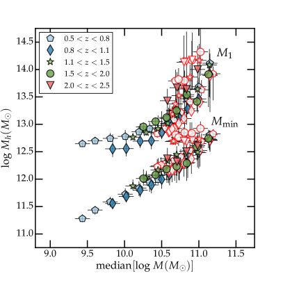
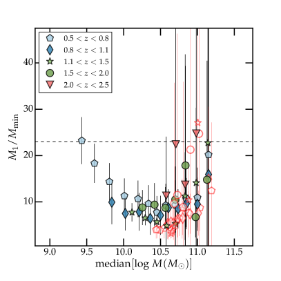
Figure 9: Characteristic halo masses $M_{\rm min}$ and $M_{\rm 1}$ (left panel) and the ratio $M_{\rm min}/M_{1}$ (right panel) as a function of sample median stellar mass threshold. Passive samples are shown in red open symbols.

We now consider the characteristic mass scales $M_{\rm min}$ and $M_{1}$, representing the minimum halo mass required to host one and two galaxies respectively. These quantities are shown in the left panel of Figure 9 as a function of median sample stellar mass for each redshift bin and mass threshold (as before, red symbols represent passive galaxy samples). As we have seen in Figures 5 and 6, galaxies with higher stellar masses reside in progressively more massive dark matter haloes. In the log-log plane of Figure 9, this is an approximately linear relationship with one important exception: the lowest-mass bin in $M_{1}$, which flattens out at lower-mass thresholds. Some hint of this is also seen in the next-nearest mass threshold, suggesting that this is a generic feature of the lower-mass threshold samples. There is some evidence in Figure 9 that, at a fixed stellar mass threshold, at low redshifts, both $M_{\rm min}$ and $M_{1}$ do not evolve: however, at $z\sim 1$ they increase sharply with redshift, as can be seen for the highest redshift bin $2.0<z<2.5$.

We now consider the “mass gap” between $M_{\rm 1}$ and $M_{\rm min}$: the right panel of Figure 9 shows the ratio $M_{\rm min}/M_{1}$. It is useful to first consider the lowest redshift bin, $0.5<z<0.8$, as this probes the largest stellar mass thresholds. We can clearly see that this ratio passes through a minimum at intermediate mass thresholds. For both low-mass and high-mass stellar masses, this ratio is $\sim 20$; at intermediate stellar mass thresholds, the ratio is $\sim 10$. This allows us to understand measurements in the literature: at high thresholds in absolute magnitude (corresponding to our most massive samples), Zehavi et al. (2011) using SDSS observations at $z\sim 0.1$ found $\sim 20$; on the other hand, Wake et al. (2011) in the NEWFIRM Medium band survey (NMBS) at $z\sim 1.5$ found much smaller values, $\sim 10$; however as we can see from Figure 9 this is primarily because these observations probed a much smaller range in stellar mass thresholds; in Figure 9, most of our observations are at this stellar mass threshold.

One interpretation of our results is that at high stellar mass thresholds, it becomes more difficult (it requires a more massive halo) to form satellites as the material preferentially falls onto the central object. There is some evidence also that that ratio between $M_{1}$ and $M_{\rm min}$ decreases towards higher redshift as a consequence of the fact $M_{1}$ evolves less rapidly than $M_{\rm min}$, although our error bars are large in the high redshift / high stellar mass bins. Kravtsov et al. (2004) used high-resolution dissipationless $N$-body simulations to investigate the halo occupation distribution and predicted that $M_{1}/M_{\rm min}$ should have $2/3$ of its $z=0$ value by $z=1$. This prediction is consistent with what we find between our redshift bins $0.5<z<0.8$ and $1.1<z<1.5$. This means that, at higher redshifts, the difference between haloes containing several galaxies or only one becomes smaller which could be seen as a evidence that, at higher redshift, haloes may have more recently accreted satellites.

5.5 The stellar-mass halo-mass relationship and comparisons with abundance-matching measurements

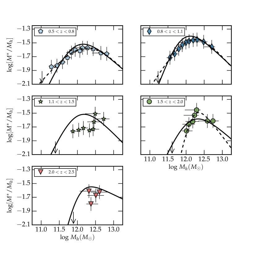
Figure 10: The ratio between the median stellar mass in each sample and the halo mass at each redshift slice (filled coloured symbols). The dotted and solid lines shows fit of the Yang et al. analytic expression to the HOD measurements and the abundance matching results. The downward-pointing arrow in each redshift slice shows our approximate completeness limit in stellar mass, translated to the corresponding halo mass at that redshift.

Previously, we have considered the relationship between the characteristic halo mass scales and each samples’ stellar mass threshold. Another way to consider this relationship is to compute the ratio of stellar mass to halo mass as a function of either halo mass or stellar mass, known as the stellar-mass halo mass relationship, or SHMR. This has the advantage of explicitly showing what fraction of mass in stars is contained within a dark matter halo of given halo mass. One may then attempt to interpret this quantity in terms of the integrated star-formation history over the lifetime of the halo, and in particular the star-formation rate per stellar mass, or the specific star-formation rate. The implication is that present-day haloes which have a higher stellar mass to halo mass relationship are those in which star-formation was more efficient than the past. Figure 10 shows, for each redshift slice, the ratio of the median stellar mass to the characteristic halo mass $M_{\rm{min}}$ as a function of halo mass.

We fit this ratio to the widely-used relationship of Yang et al. (2003) which models the SHMR as a double power-law with a different slope at high-mass and low-mass sides. Although it is has been suggested that this functional form may not be an optimal description of the SHMR (Leauthaud et al., 2011) we consider it sufficient for this current dataset, given the uncertainties which exist concerning the nature of dark matter haloes at high and intermediate redshifts which are currently not well constrained. The dashed lines show the fit to the Yang et al. relationship, where each point was weighted by the corresponding error in $M_{\rm min}$ computed by PMC fitting procedure.

For most redshift bins, our COSMOS-UltraVISTA survey provides enough low mass and high-mass haloes to constrain the SHMR on both sides of the peak. However, for the $2<z<2.5$ bin we are not able to determine the peak location, given the challenging nature of correlation function measurements over sufficiently large stellar mass range at these redshifts. This is also the case for our “outlier” bin $1<z<2$ (which we already mentioned in Section 5.3 and is discussed further in Section 5.8) for which we are not able to determine the position of the peak.

In order to constrain the peak position for all redshift bins, and to provide an additional check on the robustness of our results, we determine the peak position by using an alternative abundance matching technique (Kravtsov et al., 2004; Vale & Ostriker, 2006; Conroy et al., 2006). Essentially one matches the abundances of haloes selected in a certain way to galaxies selected in a (hopefully equivalent) way.

For our abundance matching analysis, we use a series of snapshot outputs at each of our redshift slices from a large, high resolution $N-$body dark-matter-only simulation performed with Gadget-2 (Springel, 2005) for a $\Lambda$CDM universe using Planck parameters (Planck Collaboration et al., 2014), namely $\Omega_{M}=0.307$, $\Omega_{\Lambda}=0.693$, $h=0.678$ and $\sigma_{8}=0.829$. The size of the simulation box is a cube of 80 $h^{-1}$ Mpc on a side and contains in total 1024³ particles with a mass resolution of $3\times 10^{7}M_{\odot}$ per particle. Haloes and sub-haloes are identified using the halo finding algorithm AdaptaHOP (Aubert et al., 2004) which uses an SPH-like kernel to compute densities at the location of each particle and partitions the ensemble of particles into halos and sub-haloes based on saddle points in the density field. The minimum number of particles per halo is 20: therefore, the least massive haloes in our survey ($\sim~{}10^{11}M_{\odot}$) are well resolved.

Next, circular velocities ($v_{\rm max}$) and masses ($M_{\rm 200}$) are extracted for each halo and subhalo. Circular velocities are defined as in the usual way, $V_{\rm max}=\rm max(\sqrt{Gm(\leq r)/r}\,)$, where $m(\leq r)$ is the mass enclosed at radius r. $V_{\rm max}$ can be estimated without any accurate estimate of the physical boundary of the objects which be difficult in particular for sub-haloes. For each object, we define the radius $R_{200}$ (and thus the mass $M_{200}$) as the radius where the enclosed mean density $M_{V}/(4\pi R_{V}^{3}/3)$ is $200$ times the critical density, $\rho_{c}(z)=3H(z)^{2}/8\pi G$, where $H(z)=H_{0}\sqrt{\Omega_{m}(1+z)^{3}+\Omega_{\Lambda}}$.

At each redshift bin, we determine the stellar mass threshold which matches the total abundance of galaxies selected by stellar mass $M$ to the total abundances of haloes selected by $v_{\rm max}$, i.e.,

$$N_{h}(>V_{\rm max})=N_{\rm g}(>M).$$ (17)

We compute our galaxy abundances by integrating the mass functions given in Ilbert et al. (2013). Then, at each redshift slice, we fit a simple linear function to the relationship between the median $v_{\rm max}$ and $M_{200}$ for each bin of median halo mass. This allows us in turn to derive the characteristic halo masses at each abundance threshold, and, consequently, at the corresponding stellar mass threshold. The results from this procedure are shown as the solid lines in Figure 10 (this line is actually the fit to the Yang et al. (2003) relation). At each redshift slice our simulation contains sufficient numbers of low-mass and high-mass haloes to reliably constrain the location the position of the peak in the ratio $M_{*}/M_{h}$. The arrows on each panel shows the completeness limits in stellar mass threshold presented in Figure 1.

At $z<1$ abundance matching measurements agree with our halo model measurements for higher-mass haloes: at the lower-mass end there is a slight systematic offset. We note that the halo mass function used for our halo modelling is not the same as the halo mass function in our HOD model. As the dark matter halo mass function as these redshifts is not constrained by observations, it is difficult to choose between these two mass functions. We note that in the high mass regime, the two methods are in good agreement, suggesting that $M_{\rm min}$ and $M_{\rm 200}$ are equivalent estimates of halo mass.

As before, each redshift bin, we fitted the position of the peak using the Yang et al. analytic expression. These points are shown as the open symbols in Figure 11, slightly offset for clarity. Figure 11 also includes a selection of literature measurements. We note the large scatter between previous measurements, which is probably related either to the measurement technique or the sample selection. Most lower-redshift samples, with the exception of (Leauthaud et al., 2011), are luminosity-selected and not mass-selected, and the conversion to a reliable mass-selected sample is uncertain (see Figure 14. in Coupon et al. for an idea of the typical uncertainties).

We should also note that in this work we compute the dark matter halo masses given a sample of galaxies selected by stellar mass. Works such as Leauthaud et al. (2012) actually calculate stellar mass content for a given halo mass. In the case of large scatter between stellar mass and halo mass, these two measurements may not be equivalent.

In this work, our measurements are always made for highly complete samples. Stellar mass errors can potentially have an effect on the derived SHMR. This effect has been treated in detail in Behroozi et al. (2010). The effect of stellar mass errors on derived mass function in this present data set has been described in detail in Ilbert et al. (2013). The most pernicious effect is the “Eddington Bias” (Eddington, 1913) which can affect the high mass end of the stellar mass function. Figure A2 in Ilbert et al. shows that a simple gaussian description of stellar mass errors $\sigma=0.04*(1.+z)$ results in at most a 0.1-0.2 dex overestimate in stellar mass functions due to in only the most massive bins ($\log(M_{\ast}/M_{\odot})\sim 12$) – and in these bins there are not sufficient numbers of galaxies to measure correlation functions.

In summary, neither our HOD measurements nor our abundance matching indicates an evolution in the position of $M_{\rm peak}$ as a function of redshift, as have been claimed by previous authors (although, of course, a small increase with redshift cannot be ruled out by our measurements). The implication of this result will be discussed in subsequent sections.

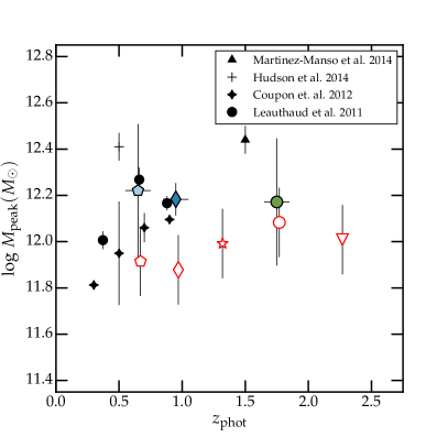
Figure 11: Location of the maximum in $M^{*}/M_{h}$ from the HOD fitting procedure (filled coloured symbols) and for the abundance matching (open red symbols). Also shown are a selection of literature results. For clarity, the abundance matching measurements are slightly offset in redshift from the HOD points.

5.6 The satellite fraction and its evolution with redshift

The physical properties of satellite galaxies (i.e., galaxies less massive than the central galaxy but lying inside the same dark matter halo) can provide additional information concerning the evolutionary history of the host dark matter halo. It is now relatively well established from both numerical simulations and observations that physical processes can modify the number of satellite galaxies. Major or minor mergers also play a role in affecting the satellite fraction. Furthermore, it seems that at $z<1$, galaxy evolution is mostly “secular”, and major mergers may not be significant (López-Sanjuan et al., 2011). At these lower redshifts however “environmental quenching” processes (Bundy et al., 2005; Peng et al., 2010) may modify the low-mass end of the global mass function. However, the rapid evolution in the global normalisation of the stellar mass functions between $1<z<2$ indicates that merging is an important process at higher redshifts, and suggest that the satellite fractions in low-redshift and high-redshift regimes should be different. From our halo occupation distribution model, we can derive the fraction of galaxies in a given dark matter halo which are satellite galaxies (Equation 13). It still remains to be seen what is the link between satellite fractions derived directly from spectroscopically identified groups Kovac et al. (2014) and measurements made such as these: it is only possible to compare these independent results to ours over a very limited range in halo mass.

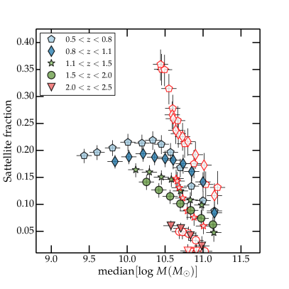
Figure 12: The satellite fraction as a function of median stellar mass threshold for the full sample and for the passive galaxy sample (open symbols).

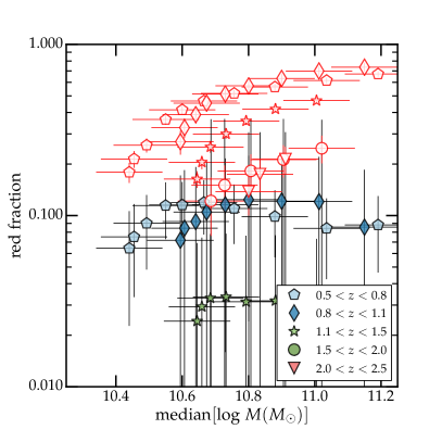
Figure 13: The fraction of the total galaxy population which are passive (filled symbols) compared with the fraction of the total galaxy population which are passive satellites (open red symbols).

Figure 12 shows the satellite fraction $f_{s}$ as a function of the stellar mass for each redshift bin for both the passive galaxy sample and the full sample. At all redshifts, the satellite fraction decreases as the stellar mass threshold increases. We also note that at lower redshift bins, at a fixed stellar mass threshold, the satellite fraction at intermediate stellar masses ($\log(M_{\ast}/M_{\odot})\sim 10.0-10.5$) is higher in the quiescent sample than in the full one. This trend is not seen at higher stellar masses, where the satellite fraction remains low, regardless of the galaxy type.

This trend is reversed above $z>1$, where the fraction of satellites is lower in quiescent galaxies populations than in the full sample. The trends in satellite fractions seen here with selection by mass and star-formation activity at low redshifts are broadly consistent with those seen in Coupon et al. (2012) and Tinker et al. (2013), although the former study made selections in “corrected” luminosity and rest-frame colour. Our measurements are below those of Wake et al. (2011); they fixed $\alpha$ in Equation 13 to one while in our case it is treated as a free parameter. This flattening in the satellite fraction was also observed by Wake et al. (2011), Zehavi et al. (2011) and Zheng et al. (2007).

Since we know the fraction of satellite galaxies for both the full population and the passive population, we can compute the fraction of the total galaxy population which is a “passive satellite” and also (using the total number of galaxies) the fraction of passive galaxies. Figure 13 shows the fraction of the total galaxy population which is passive (open red symbols) and the fraction of total galaxy population which are passive satellite galaxies (filled symbols). The dependence of the passive fraction on mass is simply a reflection of the well-known result that the peak in the number of quiescent galaxies is at $z\sim 0.8$. This is to some extent mirrored in the evolution of the fraction of passive satellite galaxies, which tracks the overall passive galaxy population. In all cases, the fraction of passive satellite galaxies drops steeply at higher redshifts. Taken together, these trends suggest that massive galaxies at high redshifts may have already accreted all their satellites.

5.7 Galaxy bias

Galaxies are not perfect tracers of the underlying dark matter distribution. (Depending on one’s viewpoint, this may be regarded either as a “nuisance parameter” or containing information concerning galaxy evolution.) A knowledge of galaxy bias has become important in calibrating accurately cosmological probes, and so we now turn to a determination of galaxy bias in our survey using the halo model.

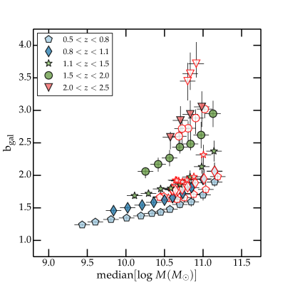
Figure 14: The galaxy bias for each redshift slice for the full and quiescent samples (filled and red open symbols respectively) as a function of median stellar mass and for each redshift slice.

The well-known dependence of galaxy bias on luminosity has been studied extensively both in the local Universe and at higher redshifts (Norberg et al., 2001; Zehavi et al., 2011; Pollo et al., 2006; Coil et al., 2008; Meneux et al., 2009; Marulli et al., 2013). Photometric surveys have also provided important information at higher redshifts (McCracken et al., 2008; Coupon et al., 2012). The consensus from these studies is that that bias is a weak function of luminosity for galaxies with $L<L_{\ast}$ (where $L_{\ast}$ is the characteristic luminosity from the Schechter function) and increases steeply for $L>L_{\ast}$. Interpreting these bias measurements has not always been straightforward, because in luminosity-selected surveys substantial luminosity evolution with redshift complicates our understanding of the relationship between mass in stars and galaxy mass. It is only very recently that it has been possible to make bias measurements as a function of stellar mass for a statistically significant volume.

Figure 14 shows the galaxy bias derived from our best-fitting halo model parameters (see Equation 12) as a function of the stellar mass at each redshift bin. We see a monotonic trend that bias increases with redshift as in Arnalte-Mur et al. (2014) for example. For $z\leq 1$, and for stellar masses less than $10^{10.7}M_{\sun}$ for the full sample and for $10^{10.7}M_{\sun}$ for the quiescent sample, the bias depends weakly on stellar mass. However at stellar masses $10^{10.7--10.9}M_{\sun}$ bias is a strong function of stellar mass. For low stellar mass threshold full galaxy samples selected at low redshift we find $b_{gal}\sim 1.3$; the quiescent population is more strongly biased $b_{gal}\sim 1.6$. in agreement with the CFHTLS and PRIMUS Coupon et al. (2012); Skibba et al. (2013).

Our data provides the most reliable measurement to date of the bias of quiescent galaxy populations at high redshifts: at $2.0<z<2.5$ we find $b_{\rm gal}\sim 3.5$ for the quiescent galaxy population, and $b_{\rm gal}\sim 3$ for the full galaxy population. We note also that the difference in bias between the full galaxy population and the quiescent population at the same stellar mass threshold increases at higher redshifts. This is almost certainly because the full galaxy population is dominated by star-forming galaxies at high redshifts, which are weakly clustered, a point to which we will return to in the discussion Section.

5.8 On the representativeness of the COSMOS field and a comparison with other results

It has already been noted that there are an overabundance of rich structures in the cosmos field (Meneux et al., 2009; McCracken et al., 2007), particularly at $z\sim 1$. In fact, some earlier studies such as Meneux et al. failed to find any significant dependence of clustering on stellar mass threshold, which in all likelihood due to their relatively bright threshold in stellar mass, but also to the overabundance of rich clusters in the field. More speculatively, the discovery of a “quasar wall” a few degrees away from the COSMOS field which may in part give rise to the overal increase in density in the COSMOS field (Clowes et al., 2013). However, despite this overall slightly elevated density increase, most of the relations presented in previous sections are qualitatively in agreement with what one expect, with the exception of the redshift bin at $1<z<1.5$ which deviates markedly and consistently from all trends presented in this paper.

To investigate further the discrepancy at $1<z<1.5$ we used the “WIRDS” data set (Bielby et al., 2012) to investigate the nature of the differences between COSMOS and other data. Although WIRDS is shallower than the present data set, it consists of four fields separated widely on the sky. We measured correlation functions in averaged mass-thresholded data in WIRDS and compared it to the COSMOS field. Interestingly, we find that the WIRDS data agrees with COSMOS on large scales, but a small scales there is much more power in COSMOS than in WIRDS. The implication which this has in the halo model fits can be seen in Figure 8: for a given abundance, the derived halo masses are much lower than one would expect, essentially because of the much steeper one-halo term. This has implications for any study using the COSMOS field to measure small scale clustering at $1<z<1.5$. For example, the very steep two-point correlation function measured in (McCracken et al., 2010; Béthermin et al., 2014) at $1<z<1.5$ seems now to be an artefact of very rich, small scale clustering present at this redshift bin.

6 Discussion: the changing relationship between galaxies and the dark matter haloes they inhabit

To understand the results presented in the previous Sections they need to be considered in the general context of the evolution of the galaxy population from $z\sim~{}0$ to $z\sim 2$, some aspects of which are now quite well understood. Of course, the precise mechanisms which give rise to these changes is still debated, but we can at least consider how our abundance and halo mass measurements reflect these well-established changes in the global galaxy population.

It is worth starting by reminding ourselves of the evolution observed in the stellar mass function from $z\sim 0$ to $z\sim 2$ for both passive and full galaxy populations. As described in Ilbert et al. (2013) (based on measurements made in these data), the total normalisation of the global mass function increases steadily from $z\sim 2$ to $z\sim 0$. However, for the passive galaxy population a rapid build-up is observed in the faint-end slope below $z\sim 1$. We may also consider the evolution of the amount of star-formation per unit mass (sSFR), the specific star formation rate, sSFR. At a given stellar mass, the sSFR declines steadily until $z\sim 0$ (Ilbert et al., 2013): stated another way, star formation at high redshift occurs preferentially in higher-mass systems. The implications for the results presented here are several: firstly, at a fixed stellar mass threshold, the proportions of passive and star-forming galaxies is a strong function of redshift and stellar mass. At high redshifts ($z\sim 2$), our mass-selected samples are dominated by star-forming massive galaxies; at low redshifts, in contrast, the low-mass end becomes increasingly dominated by passively-evolving galaxies. How may we understand our results in terms of these changes in the global galaxy population?

Firstly, it is interesting to consider the dependence of clustering amplitude on stellar mass and redshift. Our measurements show clearly the dependence of galaxy clustering on stellar mass threshold. It is interesting to note that the weak dependence of clustering strength on stellar mass for the passive galaxy population in our threshold samples at $z\sim 0.8$ is entirely due to the large “lump” of passively-evolving galaxies at $M\sim 10^{10.5}$ $M_{\sun}$ visible in the mass-redshift plane (Figure 1): changes in the threshold do not change the number of lower mass galaxies in the sample. Over the large redshift range of our survey, at a fixed stellar mass, the projected clustering amplitude at a fixed stellar mass threshold drops significantly. This is in due part a simple projection effect (and note also that at higher redshifts, our redshifts bins are larger) as our co-moving correlation lengths at fixed stellar mass, measured using our halo model, remain remarkably constant (Figure 7). The increasingly biased nature of the galaxy population, (Figure 14) is almost perfectly offset by the decreasing clustering amplitude of the underlying dark matter.

We fit our observations to a phenomenological halo model. Previously, Coupon et al. found that the fitted parameters of this model changed remarkably little from $z\sim 1$ to $z\sim 0$, reflecting the nature of the changes taking place in the galaxy population over this redshift range. This is certainly not the these data: above $z>1$, many aspects of the fitted model parameters change radically. At fixed abundance, characteristic halo masses drop significantly above $z>1$ (Figure 8). The mass fraction of satellite galaxies contained in haloes drops almost to zero, and this effect is ever more pronounced for the passive galaxy population. In addition, the fraction of mass in satellite galaxies for faint passively-evolving galaxies rises rapidly for faint galaxies (one sees almost exactly the same effect if one considers these quantities as a function of halo mass). It is challenging to compare the satellite fractions measured in previous works (Kovac et al., 2014) because of the different mass ranges probed with respect to spectroscopic surveys. However, qualitatively, this behaviour is in agreement with what one would expect from our current hierarchical models of galaxy evolution, where at high redshifts dark matter haloes are dominated by single massive galaxies. The rapid increase in the satellite fraction for faint passive galaxies happens exactly at the redshift range where the faint end of the mass function rises sharply and “satellite quenching” processes become a dominant process in galaxy evolution (Peng et al., 2010).

Considering the differences between the passive and total galaxy population, it is interesting to note that passive galaxies and the full galaxy population lie on the same halo mass / abundance relationship (Figure 8), and occupy the same region of parameter space as “normal” galaxies. In almost all of the plots presented in this paper, the passive galaxy sample occupies the same region of parameter space as a less abundant, more clustered version of the full galaxy sample with one important exception: the satellite fraction, where the passive population is revealed as radically different from the full galaxy population.

We also consider the ratio between stellar mass and halo mass for a range of halo masses in each of our redshift slices. We find that the peak position shows only a weak dependence on redshift. This is a natural consequence of the fact that the shape of the overal stellar mass function and halo mass function evolves little from $z\sim 2$ to the present day. We compared our halo model measurements with the results of an abundance matching technique and find approximately the same behaviour. The abundance matching measurements allow us estimate $M^{*}/M_{h}$ ratios even for redshifts bins for which we are not able to fit our halo model results. In general, results are broadly in agreement with models which attempt to model jointly with the evolution of the stellar mass function over large redshift baseline. For example (Behroozi et al., 2013) find only a small increase in characteristic halo mass with redshift.

7 Conclusions

We have used highly precise photometric redshifts in the UltraVISTA-DR1 near-infrared survey to investigate the changing relationship between galaxy stellar mass and the dark matter haloes hosting them to $z\sim 2$. We have achieved this by measuring the clustering properties and abundances of a series of volume-limited galaxy samples selected by stellar mass and star-formation activity. These measurements span a uniquely large range in stellar mass and redshift and reach below the characteristic stellar mass to $z\sim 2$.

We found the following results: 1. At fixed redshift and scale, clustering amplitude depends monotonically on sample stellar mass threshold; 2. At fixed angular scale, the projected clustering amplitude decreases with redshift but the co-moving correlation length remains constant; 3. Characteristic halo masses and galaxy bias increase with increasing median stellar mass of the sample; 4. The slope of these relationships is modified in lower mass haloes; 5. Concerning the passive galaxy population, characteristic halo masses are consistent with a simply less-abundant version of the full galaxy sample, but at lower redshifts the fraction of satellite galaxies in the passive population is very different from the full galaxy sample; 6. Finally we find that the ratio between the characteristic halo mass and median stellar mass at each redshift bin reaches a peak at ${\log(M_{h}/M_{\odot})}\sim 12.2$ and the position of this peak remains constant out to $z\sim 2$. The behaviour of the full and passively evolving galaxy samples can be understood qualitatively by considering the slow evolution of the characteristic stellar mass in the redshift range covered by our survey.

The next step is to extend this analysis to higher redshifts ($z>4$), where the discrepancy between models of galaxy formation and observations becomes even more acute. The new UltraVISTA DR2 data release, reaching several magnitudes deeper in all near-infrared bands, will enable for the first time this kind of study.

8 Acknowledgments

HJM acknowledges financial support form the “Programme national cosmologie et galaxies” (PNCG). This work is based on data products from observations made with ESO Telescopes at the La Silla Paranal Observatory under ESO programme ID 179.A-2005 and on data products produced by TERAPIX and the Cambridge Astronomy Survey Unit on behalf of the UltraVISTA consortium. JSD acknowledges the support of the European Research Council via the award of an Advanced Grant, and the contribution of the EC FP7 SPACE project ASTRODEEP (Ref.No: 312725).

¹ Institut d’Astrophysique de Paris, Université Pierre et Marie Curie - Paris 6, 98 bis Boulevard Arago, F-75014 Paris, France ²Institute for Astronomy, University of Hawaii, 2680 Woodlawn Drive, Honolulu, HI, 96822
³CEA Saclay, Service d’Astrophysique (SAp), Orme des Merisiers, Bât. 709, 91191 Gif-sur-Yvette, France
⁴Laboratoire d’Astrophysique de Marseille, UMR 7326, 38 rue Frédéric Joliot-Curie, 13388 Marseille cedex 13, France
⁵ Astronomical Observatory of the University of Geneva, ch. d’Ecogia 16, 1290 Versoix, Switzerland
⁶ SUPA, Institute for Astronomy, University of Edinburgh, Royal Observatory, Edinburgh EH9 3HJL, UK
⁷ Dark Cosmology Centre, Niels Bohr Institute, University of Copenhagen, Juliane Maries Vej 30, 2100 Copenhagen, Denmark
⁸ Kapteyn Astronomical Institute, University of Groningen, P.O. Box 800, 9700 AV Groningen, The Netherlands
⁹ European Southern Observatory, Karl-Schwarzschild-Str. 2, 85748 Garching, Germany

References

- Arnalte-Mur et al. (2014) Arnalte-Mur P. et al., 2014, MNRAS, 441, 1783
- Aubert et al. (2004) Aubert D., Pichon C., Colombi S., 2004, MNRAS, 352, 376
- Behroozi et al. (2010) Behroozi P. S., Conroy C., Wechsler R. H., 2010, ApJ, 717, 379
- Behroozi et al. (2013) Behroozi P. S., Wechsler R. H., Conroy C., 2013, ApJ, 770, 57
- Benjamin et al. (2010) Benjamin J., Van Waerbeke L., Ménard B., Kilbinger M., 2010, MNRAS, 408, 1168
- Béthermin et al. (2014) Béthermin M. et al., 2014, A&A, 567, A103
- Bielby et al. (2012) Bielby R. et al., 2012, A&A, 545, 23
- Bielby et al. (2014) Bielby R. M. et al., 2014, A&A, 568, A24
- Bruzual & Charlot (2003) Bruzual G., Charlot S., 2003, MNRAS, 344, 1000
- Bruzual & Charlot (2003) Bruzual G., Charlot S., 2003, MNRAS, 344, 1000
- Bundy et al. (2005) Bundy K., Ellis R. S., Conselice C. J., 2005, ApJ, 625, 621
- Capak et al. (2007) Capak P. et al., 2007, ApJS, 172, 99
- Chabrier (2003) Chabrier G., 2003, \pasp, 115, 763
- Clowes et al. (2013) Clowes R. G., Harris K. A., Raghunathan S., Campusano L. E., Sochting I. K., Graham M. J., 2013, MNRAS, 429, 2910
- Coil et al. (2008) Coil A. L. et al., 2008, ApJ, 672, 153
- Conroy & Wechsler (2009) Conroy C., Wechsler R. H., 2009, ApJ, 696, 620
- Conroy et al. (2006) Conroy C., Wechsler R. H., Kravtsov A. V., 2006, ApJ, 647, 201
- Cooray & Sheth (2002) Cooray A., Sheth R., 2002, Phys.Rev, 372, 1
- Coupon et al. (2009) Coupon J. et al., 2009, A&A, 500, 981
- Coupon et al. (2012) Coupon J. et al., 2012, A&A, 542, A5
- Cowie et al. (1996) Cowie L. L., Songaila A., Hu E. M., Cohen J. G., 1996, Astronomical Journal v.112, 112, 839
- Croton et al. (2007) Croton D. J., Gao L., White S. D. M., 2007, MNRAS, 374, 1303
- Daddi et al. (2004) Daddi E., Cimatti A., Renzini A., Fontana A., Mignoli M., Pozzetti L., Tozzi P., Zamorani G., 2004, ApJ, 617, 746
- Davis et al. (2003) Davis M. et al., 2003, Discoveries and Research Prospects from 6- to 10-Meter-Class Telescopes II. Edited by Guhathakurta, 4834, 161
- Eddington (1913) Eddington A. S., 1913, MNRAS
- Foucaud et al. (2010) Foucaud S., Conselice C. J., Hartley W. G., Lane K. P., Bamford S. P., Almaini O., Bundy K., 2010, MNRAS, 406, 147
- Groth & Peebles (1977) Groth E. J., Peebles P. J. E., 1977, ApJ, 217, 385
- Guzzo et al. (2014) Guzzo L. et al., 2014, A&A, 566, A108
- Hoaglin et al. (1983) Hoaglin D. C., Mosteller F., Tukey J. W., 1983, Understanding robust and exploratory data anlysis
- Ilbert et al. (2006) Ilbert O. et al., 2006, A&A, 457, 841
- Ilbert et al. (2013) Ilbert O. et al., 2013, A&A, 556, A55
- Ilbert et al. (2010) Ilbert O. et al., 2010, ApJ, 709, 644
- Kilbinger et al. (2010) Kilbinger M. et al., 2010, MNRAS, 405, 2381
- Kovac et al. (2014) Kovac K. et al., 2014, MNRAS, 438, 717
- Kravtsov et al. (2004) Kravtsov A. V., Berlind A. A., Wechsler R. H., Klypin A. A., Gottlöber S., Allgood B., Primack J. R., 2004, ApJ, 609, 35
- Landy & Szalay (1993) Landy S. D., Szalay A. S., 1993, ApJ, 412, 64
- Le Fèvre et al. (2005) Le Fèvre O. et al., 2005, A&A, 439, 845
- Leauthaud et al. (2010) Leauthaud A. et al., 2010, ApJ, 709, 97
- Leauthaud et al. (2011) Leauthaud A., Tinker J., Behroozi P. S., Busha M. T., Wechsler R. H., 2011, ApJ, 738, 45
- Leauthaud et al. (2011) Leauthaud A. et al., 2011, ApJ, 744, 159
- Leauthaud et al. (2012) Leauthaud A. et al., 2012, ApJ, 744, 159
- Limber (1954) Limber D. N., 1954, ApJ, 119, 655
- López-Sanjuan et al. (2011) López-Sanjuan C. et al., 2011, A&A, 530, A20
- McCracken et al. (2010) McCracken H. J. et al., 2010, ApJ, 708, 202
- McCracken et al. (2008) McCracken H. J., Ilbert O., Mellier Y., Bertin E., Guzzo L., Arnouts S., Le Fèvre O., Zamorani G., 2008, A&A, 479, 321
- McCracken et al. (2012) McCracken H. J. et al., 2012, A&A, 544, A156
- Marulli et al. (2013) Marulli F. et al., 2013, A&A, 557, A17
- McCracken et al. (2007) McCracken H. J. et al., 2007, ApJS, 172, 314
- Meneux et al. (2009) Meneux B. et al., 2009, A&A, 505, 463
- Moster et al. (2010) Moster B. P., Somerville R. S., Maulbetsch C., van den Bosch F. C., Macciò A. V., Naab T., Oser L., 2010, ApJ, 710, 903
- Navarro et al. (1997) Navarro J. F., Frenk C. S., White S. D. M., 1997, ApJ, 490, 493
- Neyman & Scott (1952) Neyman J., Scott E. L., 1952, ApJ, 116, 144
- Norberg et al. (2002) Norberg P. et al., 2002, MNRAS, 332, 827
- Norberg et al. (2001) Norberg P. et al., 2001, MNRAS, 328, 64
- Norberg et al. (2011) Norberg P., Gaztañaga E., Baugh C. M., Croton D. J., 2011, MNRAS, 418, 2435
- Oke (1974) Oke J. B., 1974, ApJS, 27, 21
- Peacock & Smith (2000) Peacock J. A., Smith R. E., 2000, MNRAS, 318, 1144
- Peng et al. (2010) Peng Y.-j. et al., 2010, ApJ, 721, 193
- Planck Collaboration et al. (2014) Planck Collaboration et al., 2014, A&A, 571, A16
- Polletta et al. (2007) Polletta M. et al., 2007, ApJ, 663, 81
- Pollo et al. (2006) Pollo A. et al., 2006, A&A, 451, 409
- Roche et al. (1999) Roche N., Eales S. A., Hippelein H., Willott C. J., 1999, MNRAS, 306, 538
- Scoccimarro et al. (2001) Scoccimarro R., Sheth R. K., Hui L., Jain B., 2001, ApJ, 546, 20
- Scoville et al. (2007) Scoville N. et al., 2007, ApJS, 172, 1
- Seljak (2000) Seljak U., 2000, MNRAS, 318, 203
- Sheth & Tormen (1999) Sheth R. K., Tormen G., 1999, MNRAS, 308, 119
- Skibba et al. (2013) Skibba R. A. et al., 2013, ArXiv e-prints
- Springel (2005) Springel V., 2005, MNRAS, 364, 1105
- Szalay et al. (1999) Szalay A. S., Connolly A. J., Szokoly G. P., 1999, AJ, 117, 68
- Tinker et al. (2013) Tinker J. L., Leauthaud A., Bundy K., George M. R., Behroozi P., Massey R., Rhodes J., Wechsler R. H., 2013, ApJ, 778, 93
- Tinker et al. (2005) Tinker J. L., Weinberg D. H., Zheng Z., Zehavi I., 2005, ApJ, 631, 41
- Vale & Ostriker (2006) Vale A., Ostriker J. P., 2006, MNRAS, 371, 1173
- Wake et al. (2011) Wake D. A. et al., 2011, ApJ, 728, 46
- Wraith et al. (2009) Wraith D., Kilbinger M., Benabed K., Cappé O., Cardoso J.-F., Fort G., Prunet S., Robert C. P., 2009, Phys.Rev.D, 80, 023507
- Yang et al. (2003) Yang X., Mo H. J., van den Bosch F. C., 2003, MNRAS, 339, 1057
- Zehavi et al. (2011) Zehavi I. et al., 2011, ApJ, 736, 59
- Zentner et al. (2014) Zentner A. R., Hearin A. P., van den Bosch F. C., 2014, MNRAS, 443, 3044
- Zheng et al. (2005) Zheng Z. et al., 2005, ApJ, 633, 791
- Zheng et al. (2007) Zheng Z., Coil A. L., Zehavi I., 2007, ApJ, 667, 760