Integration of rule-based models and compartmental models of neurons

Abstract

Synaptic plasticity depends on the interaction between electrical activity in neurons and the synaptic proteome, the collection of over 1000 proteins in the post-synaptic density (PSD) of synapses. To construct models of synaptic plasticity with realistic numbers of proteins, we aim to combine rule-based models of molecular interactions in the synaptic proteome with compartmental models of the electrical activity of neurons. Rule-based models allow interactions between the combinatorially large number of protein complexes in the postsynaptic proteome to be expressed straightforwardly. Simulations of rule-based models are stochastic and thus can deal with the small copy numbers of proteins and complexes in the PSD. Compartmental models of neurons are expressed as systems of coupled ordinary differential equations and solved deterministically. We present an algorithm which incorporates stochastic rule-based models into deterministic compartmental models and demonstrate an implementation (“KappaNEURON”) of this hybrid system using the SpatialKappa and NEURON simulators.

1 Introduction

The experimental phenomena of long term potentiation (LTP) and long term depression (LTD) show that synapses can transduce patterns of electrical activity on a timescale of milliseconds in the neurons they connect into long-lasting changes in the expression levels of neurotransmitter receptor proteins. This synaptic plasticity plays a crucial role in the development of a functional nervous system and in encoding semantic memories (e.g. motor patterns) and episodic memories (experiences), converting stimuli lasting for seconds into memories that last a lifetime [16].

There are a number of computational models of how synaptic plasticity arises from patterns of pre- and postsynaptic electrical activity, the dynamics of $\alpha$-amino-3-hydroxy-5-methyl-4-isoxazolepropionic acid receptors (AMPARs) and N-methyl-D-aspartic acid receptors (NMDARs), calcium influx through these receptors and intracellular signalling in the postsynaptic density (PSD), a dense, protein-rich structure attached to neurotransmitter receptors [1, 22, 14, 28]. The level of detail of the molecular component of these models ranges from deterministic simulations in one compartment [1] through stochastic models with coarse granularity [27] and, at the most detailed, particle-based simulations in which the Brownian motion of individual molecules is modelled [26, 28].

The model with the greatest number of molecular species has 75 variables representing the concentrations of signalling molecules, complexes of signalling molecules and phosphorylation states [1]. This constitutes a small subset of the 1000 proteins identified in the mouse postsynaptic proteome, the collection of proteins in the PSD [6]. Even the subset of the postsynaptic proteome containing proteins associated with membrane-bound neurotransmitter receptors contains over 100 members [20]. As these proteins are particularly associated with synaptic plasticity, it would be desirable to increase the number of proteins and complexes it is possible to describe in simulations.

As each protein has a number of binding sites, a combinatorially large number of complexes can arise, meaning that a correspondingly large number of reactions are needed to describe the dynamics of all possible complexes. By specifying rules whose elements are fragments of complexes, rule-based languages and simulators [5], such as Kappa [7] or BioNetGen [9], obviate the need to specify reactions for all possible complexes. These rules are simulated using a method similar to Gillespie’s stochastic simulation method for reactions [7]. Kappa has been used to predict the sizes of clusters of proteins in the postsynaptic proteome [23].

Compartmental models of electrical activity in neurons split the neuronal morphology into a number (ranging from 1 to around 1000) of compartments, and specify the dynamics of the membrane potential in each compartment in terms of coupled ordinary differential equations (ODEs) [12, 25]. Quantities beyond the membrane potential can also be modelled, e.g.  intracellular calcium concentration and concentrations of a few other molecules such as buffers and pumps. Various packages can generate and solve the equations underlying compartmental models from various model description languages, for example NEURON [3], MOOSE [21] and PSICS [2].

We present an algorithm which integrates rule-based models and compartmental models of neurons. To be sure of understanding a simple, yet interesting, case, we limit ourselves to considering isolated postsynaptic proteomes in a neuron of arbitrary morphology. Although of interest, we do not consider diffusion of molecules within the neuron. We implement the algorithm by incorporating the SpatialKappa rule-based simulator [24] into the NEURON simulator [3]. We validate the combined simulator (“KappaNEURON”) against stand-alone NEURON, and demonstrate how the system can be used to simulate complex models.

2 Simulation Method

2.1 The System to Be Simulated

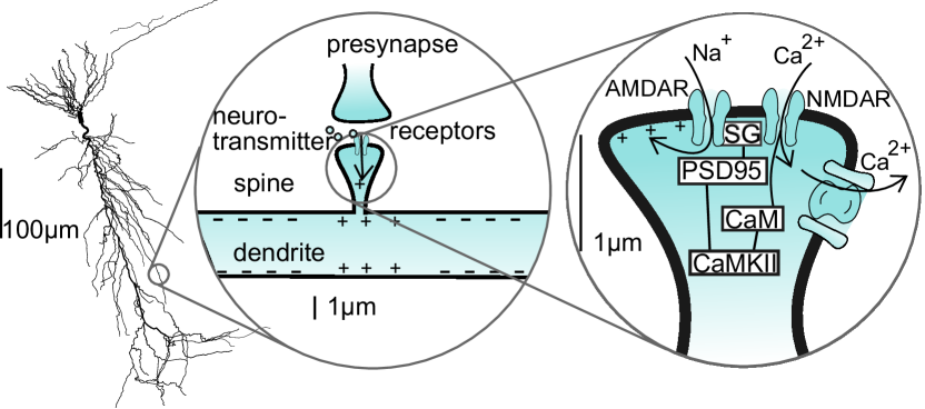
Figure 1: The system to be simulated depicted on the scale of a whole neuron (left), a spine (middle) and the postsynapse (right). Scale bars are approximate. In the postsynapse, the rectangular boxes represent intracellular molecules: SG – stargazin; CaM – calmodulin; CaMKII – Ca${}^{2}+$/calmodulin-dependent protein kinase II.

An example of the type of system to be simulated is shown in Fig. 1. There is a hippocampal CA1 pyramidal neuron (left) upon which are located a number of synapses. Excitatory synapses are generally located on synaptic spines, small protuberances from the neuron whose narrow necks limit, to an extent, diffusion of ions and molecules between the spine head and the rest of the neuron (middle). The synapse contains a postsynaptic proteome of arbitrary complexity (right). Firing in the presynaptic neuron causes release of neurotransmitter from the presynaptic bouton, which, after diffusing across the synaptic cleft, binds to AMPARs and NMDARs. The AMPARs open and close on a sub-millisecond timescale, allowing sodium ions to flow into the cell. These ions charge the membrane locally and flow to other parts of the neuron, where they also charge the membrane (middle, Fig. 1). The NMDARs open and close with slower dynamics, and allow calcium ions to flow into the spine. Inside the spine, the calcium ions bind to various proteins such as calmodulin and the resulting calcium-calmodulin complex may then bind to Ca${}^{2}+$/calmodulin-dependent protein kinase II (CaMKII), initiating signalling known to be critical for the induction of LTP and LTD.

We will first give the general set of equations that constitute a deterministic description of this type of system, then apply the general equations to a specific example, and next describe how the equations are solved. Finally we will show how we incorporate rule-based models and simulate the hybrid system.

2.2 Deterministic Description of Electrical and Chemical Activity in a Neuron

To describe electrical activity in the neuron, the neuron is split into compartments, each of which should be small enough to be approximately isopotential. Apart from the root compartment, which is located in the soma, each compartment has a parent, and a compartment may have one or more children. The equation for the membrane potential $V_{i}$ in compartment $i$ derives from Kirchoff’s current law:

$$C_{i}\frac{\mathrm{d}V_{i}}{\mathrm{d}t}=\sum_{j\in\mathcal{N}i}\frac{d_{ij}(V_{j}-V_{i})}{4R_{\mathrm{a}}l_{ij}^{2}}-\sum_{S}\left(I^{\mathrm{chan}}_{S,i}+I^{\mathrm{pump}}_{S,i}\right)-I^{\mathrm{chan}}_{\mathrm{ns},i}\enspace.$$ (1)

The left hand side is the current per unit membrane area charging or discharging the membrane; $C_{i}$ is the specific membrane capacitance in compartment $i$. The first term on the right hand side describes current flow into compartment $i$ from its neighbours $j\in\mathcal{N}_{i}$; $R_{\mathrm{a}}$ is the intracellular resistivity, $l_{ij}$ is the path length between the midpoints of $i$ and each of its neighbours $j$, and $d_{ij}$ is the mean diameter of the path. The second term on the right hand side is the total transmembrane current per unit area (referred to as current density) in compartment $i$ carried by various species of ion $S$ via ion channels ($I^{\mathrm{chan}}_{S,i}$) and membrane pumps ($I^{\mathrm{pump}}_{S,i}$), which act to maintain concentration differences between the intracellular and extracellular space. To represent “non-specific” ion currents whose concentration is not accounted for, there is final term $I^{\mathrm{chan}}_{\mathrm{ns},i}$. Here the minus sign reflects the conventions that inward current is negative and the extracellular space is regarded as electrical ground.

The current density carried by species $S$ through types $k$ of ion channel is:

$$I^{\mathrm{chan}}_{S,i}=\sum_{k}g_{ik}(O_{ik},t)f_{S,k}(V_{i},[S]_{i},[S]_{\mathrm{o}})\enspace,$$ (2)

where $g_{ik}$ is the conductance of ion channel type $k$ in compartment $i$, which may be a function of time or a state variable $O_{ik}$, and $f_{S,k}$ and is a function describing the $I$–$V$ characteristic of current flow of ions of type $S$ through channel $k$, which may depend on $[S]_{i}$, the intracellular concentration of $S$ in compartment $i$, and $[S]_{\mathrm{o}}$, the extracellular concentration of $S$, which is assumed to be constant. A normalised Goldmann-Hodgkin-Katz (GHK) current equation [25] can be used for $f_{S,k}$. For channels through which calcium flows, the typically large ratio between intracellular and extracellular calcium concentrations means this function depends quite strongly on the intracellular calcium concentration $[\mathrm{Ca}^{2+}]$, but in channels not permeable to calcium it is usual to use a linear approximation $V_{i}-E_{k}$, where $E_{k}$ is the reversal potential for that channel. By removing the dependence on intracellular concentrations $[S]_{i}$, this approximation allows currents carried by ions other than calcium to lumped together in a nonspecific ion category.

The state variable $O_{ik}$ is the number of type $k$ ion channels in compartment $i$ which are in an open conformation. It is modelled as the occupancy of a state of a Markov process with membrane potential-dependent transition rates. For small number of channels the Markov process is simulated stochastically, but with large numbers of channels the system is practically deterministic and the master equation of the Markov process is simulated using ODEs.

The dynamics of the intracellular concentrations of ions can be modelled using further ODEs. The rate of change of $[S]_{i}$ depends on $I^{\mathrm{chan}}_{S,i}$, the channel transmembrane current density carried by $S$, and consumption and release by intracellular reactions:

$$\frac{\mathrm{d}[S]_{i}}{\mathrm{d}t}=-\frac{a_{i}}{z_{S}Fv_{i}}I^{\mathrm{chan}}_{S,i}+\sum_{r}J_{S,r,i}\enspace,$$ (3)

where $a_{i}$ is the surface area of the compartment, $v_{i}$ is the volume of the compartment, $z_{S}$ is the valency of ion $S$, and $F$ is Faraday’s constant. The term $\sum_{r}J_{S,r,i}$ describes the net flux of $S$ due to intracellular reactions $r$. It arises from treating the intracellular reactions in compartment $i$ as a set of kinetic schemes:

$$r:\ce{\textit{S}+\textit{T}<->[k_{r}][k_{-r}]\mathit{S\cdot{}T}}\enspace.$$ (4)

The flux of $S$ arising from this reaction would be:

$$J_{S,r,i}=-k_{r}[S]_{i}[T]_{i}+k_{-r}[S\cdot T]_{i}\enspace.$$ (5)

The pump current $I^{\mathrm{pump}}_{S,i}$ may be defined in terms of the flux of a reaction $r$, for example:

$$I^{\mathrm{pump}}_{S,i}=\frac{z_{S}Fv_{i}}{a_{i}}J_{S,r,i}\enspace,$$ (6)

where the prefactor converts from flux to current. Thus the whole electrical and molecular system is defined by a system of ODEs.

2.3 Example Deterministic Description

To help understand the formalism above, we provide an example of a simple one-compartment system; this will also be used as the validation example in Section 4.1. There is a single compartment whose membrane contains passive (leak) channels, calcium channels, and a transmembrane calcium pump, described by the kinetic scheme:

Ca binding: $$\ce{P+Ca->[k_{1}]P.Ca}$$ (7)

Ca release: $$\ce{P.Ca->[k_{2}]P}\enspace,$$

where Ca represents intracellular calcium, P represents a pump molecule in the membrane, P.Ca is the pump molecule bound by calcium and $k_{1}$ and $k_{2}$ are rate coefficients.

We substitute $z_{\mathrm{Ca}}=2$ and the flux of the “Ca release” reaction into Equation (6) to obtain the pump current:

$$I^{\mathrm{pump}}_{\mathrm{Ca}}=k_{2}\frac{2Fv}{a}[\ce{P.Ca}]=k_{2}\frac{2Fv}{a}([\ce{P}]_{0}-[\ce{P}])\enspace,$$ (8)

where we have used the fact that the total concentration of the pump molecule $[\mathrm{P}]_{0}$ is the sum of the concentrations [P] and [P.Ca] of unbound and bound pump molecule. Since there is only a single compartment, we have dropped subscripts. The calcium channel current $I^{\mathrm{chan}}_{\mathrm{Ca}}$ flowing into the compartment is determined by Equation (2) with a constant conductance of magnitude $g_{\mathrm{Ca}}$, and the nonspecific current is used for the passive channels so that $I^{\mathrm{chan}}_{\mathrm{ns}}=g_{\mathrm{pas}}(V-E_{\mathrm{pas}})$, where $E_{\mathrm{pas}}$ is the passive reversal potential.

To construct the ODEs corresponding the kinetic scheme (7) and the expression for the pump current (8), Equation (5) is applied to the scheme to give fluxes, which, along with $I^{\mathrm{chan}}_{\mathrm{Ca}}$, $I^{\mathrm{pump}}_{\mathrm{Ca}}$ and $I^{\mathrm{chan}}_{\mathrm{ns}}$, are substituted in Equations (1) and (3) to give:

$$C\frac{\mathrm{d}V}{\mathrm{d}t} =-g_{\mathrm{Ca}}f_{\mathrm{Ca}}(V,[\ce{Ca}],[\ce{Ca}]_{\mathrm{o}})-k_{2}\frac{2Fv}{a}([\ce{P}]_{0}-[\ce{P}])-g_{\mathrm{pas}}(V-E_{\mathrm{pas}})$$ (9)

$$\frac{\mathrm{d}[\ce{Ca}]}{\mathrm{d}t} =-\frac{a}{2Fv}g_{\mathrm{Ca}}f(V,[\ce{Ca}],[\ce{Ca}]_{\mathrm{o}})-k_{1}[\ce{Ca}][\ce{P}]$$ (10)

$$\frac{\mathrm{d}[\ce{P}]}{\mathrm{d}t} =-k_{1}[\ce{Ca}][\ce{P}]+k_{2}([\ce{P}]_{0}-[\ce{P}])\enspace.$$ (11)

The notional volume $v$ may describe the volume of a thin submembrane shell rather than the volume of the whole compartment. We assume that $v$ is the volume of the whole cylindrical compartment so that $a/v=4/d$, where $d$ is the diameter of the compartment.

2.4 Simulation of Deterministic Variables

Simulators of deterministic electrical and chemical activity in neurons, such as NEURON [3], solve the coupled ODEs by gathering the variables $V_{i}$, $[S]_{i}$ and other state variables into one state vector $\vec{x}$ and solving the ODE system:

$$\frac{\mathrm{d}\vec{x}}{\mathrm{d}t}=\vec{G}(\vec{x})+\vec{b}(t)\enspace,$$ (12)

where $\vec{G}(\vec{x})$ is the rate of change of each state variable and $\vec{b}(t)$ is a time dependent forcing input. In principle $\vec{G}(\vec{x})$ depends on all variables, though the structure of compartmental models means each element of $\vec{G}(\vec{x})$ depends on only a few elements of $\vec{x}$. These equations can be solved by implicit Euler integration, which, although not providing the second-order accuracy of more advanced schemes, does give guarantees about numerical stability and is used by default in NEURON [18]. In implicit Euler the derivative is evaluated at $t+\Delta t$, the end of the time step:

$$\frac{\vec{x}(t+\Delta t)-\vec{x}(t)}{\Delta t}=\vec{G}(\vec{x}(t+\Delta t))+\vec{b}(t+\Delta t)\enspace.$$ (13)

Taylor expanding the right hand side of (13) in $\Delta t$ and rearranging gives the equation for one update step:

$$\vec{x}(t+\Delta t)=\vec{x}(t)+\left(I-\frac{\partial\vec{G}}{\partial\vec{x}}\Delta t\right)^{-1}\left(\vec{G}(\vec{x}(t))+\vec{b}(t)\right)\Delta t\enspace,$$ (14)

where $\partial\vec{G}/\partial\vec{x}$ is the Jacobian matrix at time $t$, which can be computed numerically, or analytically for efficiency. To optimise simulation speed, the time step $\Delta t$ may vary depending on the rate of change of the variables; but whatever the value of $\Delta t$, all variables are updated simultaneously.

2.5 Modifications to Accommodate Rule-Based Simulation

To combine fixed-step simulation of continuous variables described by ODEs with discrete variables described by stochastic, rule-based models, we use principles akin to those used in hybrid simulations of systems of chemical reactions [13]. The state variables (elements of $\vec{x}$) are partitioned into continuous variables, which are updated at fixed intervals of $\Delta t$ by an ODE solver, and discrete variables, which are updated asynchronously by the rule-based solver, as outlined in Appendix 0.A.1. Some “bridge” variables are referred to by both solvers. The combined simulation algorithm must ensure that the two solvers are synchronised appropriately and that conversions between continuous and discrete quantities are made.

For simulations combining molecular and electrical activity (e.g. Fig. 1) the membrane potential would be a continuous variable, intracellular molecules such as calmodulin and CaMKII would be stochastic variables, and the intracellular calcium in the spine would be a stochastic bridge variable.

Conversions

In deterministic simulations of biochemical reactions in neurons (e.g. [1]) a molecular species or ion $S$ is represented by an intensive quantity – its concentration $[S]$; whereas in stochastic simulations it is represented by an extensive quantity – the number of molecules $|S|$ in the volume $v$ in which $S$ exists. Thus to compare the deterministic (ODE) and stochastic (rule-based) parts of the simulation, intensive and extensive quantities need to be interconverted using Avogadro’s constant $N_{\mathrm{A}}$:

$$|S|=N_{\mathrm{A}}v[\ce{S}]\enspace.$$ (15)

Rate coefficients for reactions based on concentrations must also be converted to ones appropriate for species number for use in the rule-based simulator’s rules. To derive the conversion formula, consider a bimolecular kinetic scheme in which $k$ is the rate coefficient, i.e. S + T -¿[k] S.T. Typical units for $k$ are s . The kinetic scheme can be expressed as an ODE $\mathrm{d}[\ce{\mathit{S}.\mathit{T}}]/\mathrm{d}t=k[S][T]$. Converting the concentrations according to (15) yields an equivalent ODE whose variables are numbers of molecules: $\mathrm{d}|\ce{\mathit{S}.\mathit{T}}|/\mathrm{d}t=\gamma|S||T|$, where $\gamma=k/N_{\mathrm{A}}v$ is the converted rate coefficient and has units s . In general for an equation with $n$ reactants, the relation between rate coefficients for numbers of molecules and concentrations is $\gamma=(N_{\mathrm{A}}v)^{-n+1}k$. State variables (for example the state of channels) may also be controlled by the rule-based simulator, and here other conversion formulae apply.

Creation and Destruction Rules for Bridging Variables

To simulate the channel currents in the rule-based solver we need to write creation or destruction rules that are equivalent to $I^{\mathrm{chan}}_{S,i}$ in Equation (3). These rules are:

$$\mbox{ }\ce{->[-a_{i}\tilde{I}^{\mathrm{chan}}_{S,i}N_{\mathrm{A}}/z_{S}F]\mathit{S}} \mbox{if }\tilde{I}^{\mathrm{chan}}_{S,i}<0$$ (16)

$$\ce{\mathit{S}->[a_{i}\tilde{I}^{\mathrm{chan}}_{S,i}N_{\mathrm{A}}/z_{S}F]} \mbox{if }\tilde{I}^{\mathrm{chan}}_{S,i}>0.$$ (17)

Here $\tilde{I}^{\mathrm{chan}}_{S,i}$ can be an expression that references continuous or discrete variables.

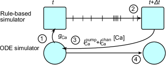
Figure 2: The update and synchronisation method. See text for explanation.

Update and Synchronisation

The procedure for updating the time from $t$ to $t+\Delta t$ (Fig. 2) is:

1. Pass all relevant continuous variables, e.g. conductances and voltages needed to compute $I^{\mathrm{chan}}_{S,i}$ in the rule-based simulator.

2. Run the rule-based simulator from $t$ to $t+\Delta t$.

3. Compute the net change $\Delta S_{i}^{\mathrm{tot}}$ in the total number of each bridging species $S$ (including in any complexes) in compartment $i$ over the time step and convert each change back to a current: $I^{\mathrm{chan}}_{S,i}+I^{\mathrm{pump}}_{S,i}=-\Delta S^{\mathrm{tot}}_{i}z_{S}F/a_{i}N_{\mathrm{A}}$. For each membrane potential $V_{i}$, set the corresponding element of $\vec{b}(t)$ equal to $-(1/C_{i})\sum_{S}({I^{\mathrm{chan}}_{S,i}+I^{\mathrm{pump}}_{S,i}})$ (see second term on right of Equation 1).

4. Update the continuous variables according to the update step (14).

When running the rule-based model, it will not stop precisely on the boundary of the time step since the update times are generated stochastically. To deal with this problem, the time of the next event in the rule-based component is computed before updating the variables. As soon as the next event time is after the end of the deterministic step, that event is thrown away, as justified in Appendix 0.A.2.

## File caPump.ka - Simple calcium pump

## Agent declarations, showing the agent names and binding sites
%agent: ca(x)   # Calcium with binding site
%agent: P(x)    # Pump molecule with binding site

## Variable declarations
%var: ’vol’ 1          # Volume in um3
%var: ’NA’  6.02205E23 # Avagadro’s constant
# Concentration of one agent in the volume in mM
%var: ’agconc’ 1E18/(’NA’ * ’vol’)
# Rate constants in /mM-ms or /ms, depending on the number of
# complexes on LHS of rule
%var: ’k1’ 0.001       # /mM-ms
%var: ’k2’ 1           # /ms

## Rules
# Note the scaling of the rate constant of the bimolecular reaction
’ca binding’ ca(x), P(x)     -> ca(x!1), P(x!1) @ ’k1’ * ’agconc’
’ca release’ ca(x!1), P(x!1) -> P(x)            @ ’k2’

## Initialisation of agent numbers
# Overwritten by NEURON but needed for SpatialKappa parser
%init:  1000 ca(x)
%init: 10000 P(x)

## Observations
%obs: ’ca’   ca(x)           # Free Ca
%obs: ’P-Ca’ ca(x!1), P(x!1) # Bound Ca-P
%obs: ’P’    P(x)            # Free P

Figure 3: Example of a Kappa file for a simple calcium pump (7) simulated in a volume of 1 µ m ^ 3 . Note the conversion of the forward rate coefficient from units of m m s  to m s . For an introduction to the Kappa language, see the short description at http://www.kappalanguage.org/syntax.html.

from neuron import *
import KappaNEURON

## Create a compartment
sh = h.Section()
sh.insert(’pas’)                # Passive channel
sh.insert(’capulse’)            # Code to give Ca pulse
# This setting of parameters gives a calcium influx and pump
# activation that is scale-independent
sh.gcalbar_capulse = gcalbar*sh.diam

## Define region where the dynamics will occur (’i’ means intracellular)
r = rxd.Region([sh], nrn_region=’i’)

## Define the species, the ca ion (already built-in to NEURON), and the
## pump molecule. These names must correspond to the agent names in
## the Kappa file.
ca = rxd.Species(r, name=’ca’, charge=2, initial=0.0)
P  = rxd.Species(r, name=’P’,  charge=0, initial=0.2)

## Create the link between the Kappa model and the species just defined
kappa = KappaNEURON.Kappa(membrane_species=[ca], species=[P],
                          kappa_file=’caPump.ka’, regions=[r])

## Transfer variable settings to the kappa model
vol = sh.L*numpy.pi*(sh.diam/2)**2
kappa.setVariable(’k1’,  47.3)
kappa.setVariable(’k2’,  gamma2)
kappa.setVariable(’vol’, vol)

## Run
init()
run(30)

Figure 4: Extract of Python code to link the Kappa file shown in Fig. 3 into a compartment in NEURON.

3 Implementation

We have implemented the algorithm described in the previous section by linking the Java-based SpatialKappa implementation of the Kappa language [24] to version 7.4 of NEURON, which allows reaction-diffusion equations to be specified in Python [18]. Our implementation (“KappaNEURON”) is available at http://github.com/davidcsterratt/KappaNEURON. We have used the py4j package to extend the SpatialKappa simulator so its Java objects can be accessed in Python. The wrapper system in NEURON 7.4 allows us to override NEURON’s built-in fixed solve callback function with one that calls the SpatialKappa simulator at each time step, as described in the previous section.

In order to specify a model the Kappa component is specified in a separate file. Fig. 3 shows an example of a simple calcium pump specified in Kappa. This file is then linked into the NEURON simulation as demonstrated in the Python code in Fig. 4. The mechanisms specified in the Kappa file take over all of NEURON’s handling of molecules in the cytoplasm of chosen sections.

4 Results

4.1 Validation

We validated our implementation by comparing the results of simulating ODE and rule-based versions of the model described in Section 2.3 using standard NEURON and KappaNEURON respectively. Fig. 5A shows the deterministic solution of the system of ODEs (9)–(11) (blue) and a sample rule-based solution using the Kappa rules in Fig. 3 (red) from a single compartment with diameter 1 µ m  and length 1 µ m , giving a volume within the range 0.01–1 µ m ^ 3 typical of spine heads in the vertebrate central nervous system [11].

A

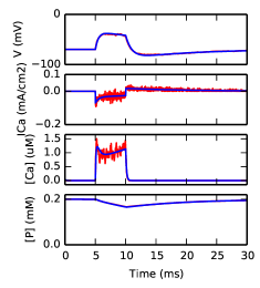
B

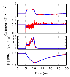
Figure 5: Reference simulations. A, Traces generated by NEURON with NMODL (blue) and KappaNEURON (red) when the diameter is 1 µ m . B, The same simulations but with a diameter of 0.2 µ m . There is more noise evident in the combined simulation due to the smaller number of ions involved.

The calcium conductance $g_{\mathrm{Ca}}$ is zero apart from during a pulse lasting from 5–10 m s  when an inward calcium current begins to flow ($I^{\mathrm{chan}}_{\mathrm{Ca}}$ is negative). This causes a sharp rise in intracellular calcium concentration [Ca], which, because of the GHK current equation, reduces the calcium current slightly, accounting for the initially larger magnitude of the calcium current. As the calcium concentration increases, it starts binding to the pump molecules, depleting the amount of the free pump molecules [P]. Once the calcium channels close ($g_{\mathrm{Ca}}=0$), the calcium influx stops, and the remaining free calcium is taken up quickly by the pumps. The pump-calcium complex dissociates at a slower rate, leading to a positive (outwards) calcium current. The stochastic traces (red) are very similar to their deterministic counterparts (blue) apart from some random fluctuations, particularly in the trace of calcium. This agreement, along with a suite of simpler tests included with the source code, indicates that the implementation is correct.

Fig. 5B shows deterministic (blue) and stochastic (red) simulations in a spine with a diameter of 0.2 µ m  (i.e. 1/25 of the volume of the simulation in Fig. 5A). The shape of the traces differs due to the change in surface area to volume ratio. Due to the smaller volume and hence smaller numbers of ions involved, the fluctuations are relatively bigger.

4.2 Demonstration Simulation

To demonstrate the utility of integrated electrical and rule-based neuronal models, we constructed a model of a subset of the synaptic proteome, with a focus on the signal processing at the early stages of the CaM-CaMKII pathway. We encoded in Kappa published models of: the dynamics of NMDARs [27]; binding of calcium with calmodulin and binding of calmodulin-calcium complexes to CaMKII [19]; and binding of calcium to a calbindin buffer [8]. We embedded these linked models into a simple model of a synaptic spine, comprising head and neck compartments, connected to a dendrite. As well as the NMDARs, modelled in Kappa, there were AMPARs in the spine head, and backpropagating spikes were modelled by inserting standard Hodgkin-Huxley ion channels [12] in the dendritic membrane. To emulate spike-timing dependent synaptic plasticity protocols [15], a train of 10 excitatory postsynaptic potentials (EPSPs) were induced in the synapse in the spine head at 20Hz, each of which was followed by an action potential. There were also 50 other synaptic inputs onto the dendrite, though these did not contain the rule-based model.

A

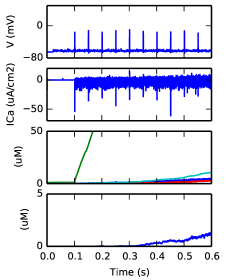
B

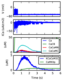
Figure 6: Demonstration simulations. A, The first 600ms of the simulation. B, The first 6000ms of the simulation. Labels: Ca, free calcium; CaCB, calcium bound to calbindin; CaCaMN, calcium bound to the N lobe of calmodulin; CaCaMC, calcium bound to the C lobe of calmodulin; KCaCaM2C, CaMKII bound to calmodulin with two calcium ions on its C lobe; and CaMKIIp, phosphorylated CaMKII.

Fig. 6 shows results from one simulation at short (0.6s) and long (6s) time scales. The first stimulation of the detailed synapse paired with action potential initiation occurs at 0.1s, as can be seen by the voltage trace. The stimulation releases glutamate, which binds to AMPARs (which remain open for a few milliseconds) and NMDARs (which remain open for 100s of milliseconds). Due to the backpropagating action potentials releasing the voltage-dependent block of NMDARs, there are peaks in the calcium current ($I_{\mathrm{Ca}}$) at the same time as the action potentials. The calcium entering through the NMDARs binds to the calbindin and calmodulin (CaM) buffers. The CaM-Ca²⁺ complex can bind to CaMKII, the rate depending on which of the C and N lobes of CaM the Ca²⁺ are bound to. This CaMKII-CaM-Ca²⁺ complex can then be phosphorylated, leading to a long lasting elevation in its level. This will then to phosphorylate stargazin, which will help to anchor AMPARs in the membrane, thus contributing to LTP.

5 Discussion

We have presented a method for integrating a stochastically simulated rule-based model of proteins in a micron-sized region of a neuron into a compartmental model of electrical activity in the whole neuron. The rule-based component allows the biochemical interactions between binding sites on proteins to be specified using a tractable number of rules, with the simulator taking on the work of tracking which complexes are present at any point during the simulation.

Our approach is similar to that of Kiehl et al. [13] who simulated chemical reactions with a hybrid scheme. However their integration scheme synchronised at every discrete event, whereas in ours, synchronisation is driven only by the time step of the continuous simulator. This principle is appropriate for neural systems, in which we can expect many discrete events per time step.

Recently Mattioni and Le Novère [17] have integrated the ECell simulator with NEURON. Our approach is similar to theirs, though with two differences. Firstly we have integrated a rule-based simulator. This has the advantage that the interactions between the combinatorially large numbers of complexes present in the PSD can be specified using a tractable number of rules, though this limits the simulation method to the sequential style of Gillespie’s stochastic simulation algorithm, and does not allow for any of the approximations that increase the algorithm’s efficiency. Secondly Mattioni and Le Novère get the ODE-based solver to handle calcium, whereas we handle it in the rule-based solver. Our approach is less efficient computationally, but it ensures that all biochemical quantities are consistent and avoids having to make any assumptions about the relative speeds of processes.

Our approach allows us to model at a considerable level of detail. For example the conformation of NMDARs may be part of the biochemical model, allowing proteins in the PSD (e.g. calmodulin bound to calcium) to modulate the state of the channel [27]. We can also use one rule-based scheme to model both the presynapse and the postsynapse, which could help to understand transynaptic signalling via molecules such as endocannabinoids [4].

Our implementation of our algorithm is publicly available (KappaNEURON; http://github.com/davidcsterratt/KappaNEURON) and under development. The next major feature planned is making available to NEURON SpatialKappa’s capability of simulating rule-based models with voxel-based diffusion.

Appendix 0.A Appendix

0.A.1 Kappa Simulation Method

To understand the asynchronous nature of the Kappa simulation method, we first illustrate Gillespie’s direct method [10] by applying it to the kinetic scheme description of a calcium pump shown in Fig. 3A. Here Ca represents intracellular calcium, P represents a pump molecule in the membrane, P.Ca is the pump molecule bound by calcium and $k_{1}$ and $k_{2}$ are rate coefficients, which are rescaled to the variables $\gamma_{1}$ and $\gamma_{2}$ as explained in Section 2.5. To apply the Gillespie method to this scheme:

1. Compute the propensities of the reactions $a_{1}=\gamma_{1}|\ce{Ca}||\ce{P}|$ and $a_{2}=\gamma_{2}|\ce{Ca.P}|$

2. The total propensity is $A=a_{1}+a_{2}$

3. Pick reaction $\mathrm{R}_{i}$ with probability $a_{i}/A$

4. Pick time to reaction $T=-(\ln r)/A$, where $r$ is a random number drawn uniformly from the interval $(0,1)$.

5. Goto 1

Kappa uses an analogous method, but applied to rules that are currently active. Both methods are event-based rather than time-step based.

0.A.2 Justification for Throwing Away Events

To justify throwing away events occurring after a time step ending at $t+\Delta t$, we need to show that the distribution of event times (measured from $t$) is the same in two cases:

1. The event time $T$ is drawn from an exponential distribution $A\exp(-AT)$ (for $T>0$), where $A$ is the propensity.

2. An event time $T_{0}$ is drawn as above. If $T_{0}<\Delta t$, accept $T=T_{0}$ as the event time. If $T_{0}\geq\Delta t$, throw away this event time and sample a new interval $T_{1}$ from an exponential distribution with a time constant of $A$, i.e. $A\exp(-AT_{1})$. Set the event time to $T=\Delta t+T_{1}$.

In the second case, the overall distribution is:

$$P(\mbox{event at }T<\Delta t) =A\exp(-AT)$$ (18)

$$P(\mbox{event at }T\geq\Delta t) =P(\mbox{survival to }\Delta t)P(\mbox{event at }T_{1})$$

$$=\exp(-A\Delta t)A\exp(-A(T-\Delta t))$$

$$=A\exp(-AT)$$

Here we have used $T_{1}=T-\Delta t$. Thus the distributions are the same in both cases.

References

- [1] Bhalla, U.S., Iyengar, R.: Emergent properties of networks of biological signalling pathways. Science 283, 381–387 (1999)
- [2] Cannon, R.C., O’Donnell, C., Nolan, M.F.: Stochastic ion channel gating in dendritic neurons: Morphology dependence and probabilistic synaptic activation of dendritic spikes. PLoS Comput. Biol. 68, e1000886 (2010)
- [3] Carnevale, T., Hines, M.: The NEURON Book. Cambridge University Press, Cambridge, UK (2006)
- [4] Castillo, P.E., Younts, T.J., Chávez, A.E., Hashimotodani, Y.: Endocannabinoid signaling and synaptic function. Neuron 761, 70–81 (2012)
- [5] Chylek, L.A., Stites, E.C., Posner, R.G., Hlavacek, W.S.: Innovations of the rule-based modeling approach. In: Prokop, A., Csukás, B. (eds.) Systems Biology, pp. 273–300. Springer-Verlag (300)
- [6] Collins, M.O., Husi, H., Yu, L., Brandon, J.M., Anderson, C.N.G., Blackstock, W.P., Choudhary, J.S., Grant, S.G.N.: Molecular characterization and comparison of the components and multiprotein complexes in the postsynaptic proteome. J. Neurochem. 97, 16–23 (2006)
- [7] Danos, V., Feret, J., Fontana, W., Krivine, J.: Scalable simulation of cellular signaling networks. In: Shao, Z. (ed.) Programming Languages and Systems, Lecture Notes in Computer Science, vol. 4807, chap. 10, pp. 139–157. Springer, Berlin, Heidelberg (2007)
- [8] Faas, G.C., Raghavachari, S., Lisman, J.E., Mody, I.: Calmodulin as a direct detector of Ca2+ signals. Nat. Neurosci. 143, 301–304 (2011)
- [9] Faeder, J., Blinov, M., Hlavacek, W.: Rule-based modeling of biochemical systems with BioNetGen. In: Maly, I.V. (ed.) Systems Biology, Methods in Molecular Biology, vol. 500, pp. 113–167. Humana Press (2009)
- [10] Gillespie, D.: Exact stochastic simulation of coupled chemical reactions. J. Phys. Chem. 81, 2340–2361 (1977)
- [11] Harris, K.M., Kater, S.B.: Dendritic spines: Cellular specializations imparting both stability and flexibility to synaptic function. Annu. Rev. Neurosci. 17, 341–371 (1994)
- [12] Hodgkin, A.L., Huxley, A.F.: A quantitative description of membrane current and its application to conduction and excitation in nerve. J. Physiol. (Lond.) 117, 500–544 (1952)
- [13] Kiehl, T.R., Mattheyses, R.M., Simmons, M.K.: Hybrid simulation of cellular behavior. Bioinformatics 203, 316–322 (2004)
- [14] Lisman, J.E., Zhabotinsky, A.M.: A model of synaptic memory: a CaMKII/PP1 switch that potentiates transmission by organizing an AMPA receptor anchoring assembly. Neuron 312, 191–201 (2001)
- [15] Markram, H., Lübke, J., Frotscher, M., Sakmann, B.: Regulation of synaptic efficiency by coincidence of postsynaptic APs and EPSPs. Science 275, 213–215 (1997)
- [16] Martin, S.J., Grimwood, P.D., Morris, R.G.M.: Synaptic plasticity and memory: An evaluation of the hypothesis. Annu. Rev. Neurosci. 231, 649–711 (2000)
- [17] Mattioni, M., Le Novère, N.: Integration of biochemical and electrical Signaling-Multiscale model of the medium spiny neuron of the striatum. PLoS ONE 87, e66811 (2013)
- [18] McDougal, R.A., Hines, M.L., Lytton, W.W.: Reaction-diffusion in the NEURON simulator. Front. Neuroinform. 728 (2013)
- [19] Pepke, S., Kinzer-Ursem, T., Mihalas, S., Kennedy, M.B.: A dynamic model of interactions of Ca2+, calmodulin, and catalytic subunits of Ca2+/calmodulin-dependent protein kinase II. PLoS Comput. Biol. 62, e1000675 (2010)
- [20] Pocklington, A.J., Cumiskey, M., Armstrong, J.D., Grant, S.G.N.: The proteomes of neurotransmitter receptor complexes form modular networks with distributed functionality underlying plasticity and behaviour. Mol. Syst. Biol. 21 (2006)
- [21] Ray, S., Bhalla, U.S.: PyMOOSE: Interoperable scripting in python for MOOSE. Front. Neuroinform. 2 (2008)
- [22] Smolen, P., Baxter, D.A., Byrne, J.H.: A model of the roles of essential kinases in the induction and expression of late long-term potentiation. Biophys. J. 908, 2760–2775 (2006)
- [23] Sorokina, O., Sorokin, A., Armstrong, J.D.: Towards a quantitative model of the post-synaptic proteome. Mol. Biosyst. 7, 2813–2823 (2011)
- [24] Sorokina, O., Sorokin, A., Armstrong, J.D., Danos, V.: A simulator for spatially extended kappa models. Bioinformatics pp. 3105–3106 (2013)
- [25] Sterratt, D., Graham, B., Gillies, A., Willshaw, D.: Principles of Computational Modelling in Neuroscience. Cambridge University Press, Cambridge, UK (2011)
- [26] Stiles, J.R., Bartol, T.M.: Monte Carlo methods for simulating realistic synaptic microphysiology using MCell. In: De Schutter, E. (ed.) Computational Neuroscience: Realistic Modeling for Experimentalists, chap. 4, pp. 87–127. CRC Press, Boca Raton, FL (2001)
- [27] Urakubo, H., Honda, M., Froemke, R.C., Kuroda, S.: Requirement of an allosteric kinetics of NMDA receptors for spike timing-dependent plasticity. J. Neurosci. 2813, 3310–3323 (2008)
- [28] Zeng, S., Holmes, W.R.: The effect of noise on CaMKII activation in a dendritic spine during LTP induction. J. Neurophysiol. 1034, 1798–1808 (2010)