Optimal control of elliptic PDEs on surfaces of codimension 1

Abstract

We consider an elliptic optimal control problem where the objective functional contains an integral along a surface of codimension 1, also known as a hypersurface. In particular, we use a fidelity term that encourages the state to take certain values along a curve in 2D or a surface in 3D. In the discretisation of this problem, which uses piecewise linear finite elements, we allow the hypersurface to be approximated e.g. by a polyhedral hypersurface. This can lead to simpler numerical methods, however it complicates the numerical analysis. We prove a priori $L^{2}$ error estimates for the control and present numerical results that agree with these. A comparison is also made to point control problems.

1 Introduction

In this paper we consider an elliptic optimal control problem with an objective functional containing an integral over a surface of codimension 1, also known as a hypersurface. In particular, we control the state to be close to prescribed values along a curve in 2D or a surface in 3D. This differs from standard elliptic optimal control problems where typically the objective functional contains the $L^{2}$ distance between the state and the desired state over the whole domain. So for a bounded domain $\Omega\subset\mathbb{R}^{n}$ ($n=2$ or $3$) and an $n-1$ dimensional surface $\Gamma\subset\Omega$ we consider the problem:

$$\min\frac{1}{2}\int_{\Gamma}(y-g_{\Gamma})^{2}\mathrm{d}A+\frac{\nu}{2}\|\eta\|^{2}_{L^{2}(\Omega)}$$ (1.1)

subject to the state equation

$$Ay =\eta\quad\text{ in }\Omega$$ (1.2)

$$y =0\quad\text{ on }\partial\Omega$$

and the control constraints

$$a\leq\eta\leq b.$$

Here $g_{\Gamma}:\Gamma\to\mathbb{R}$ is the desired state on $\Gamma$, $\nu>0$ is the cost of control, $A$ is an elliptic operator, and $a,b\in\mathbb{R}$ with $a<b$ are lower and upper bounds for the control. We will formulate this problem precisely using function spaces in Section 3.

The motivation for the surface fidelity term is that in some applications we may only care about the state being close to given values on a small part of the domain. Controlling the state using a distributed norm over the whole domain gives weaker control on the surface. Instead of this fidelity term we could use state constraints to force the state to take certain values, however this would lead to an optimal control with very high cost. The surface fidelity term allows for a compromise between how close the state is to the desired values on the surface and the cost of the control.

We have not seen the surface fidelity term previously used in the optimal control context in the literature, however other problems have been considered where the state is controlled on small sets. The book [23] formulates an optimal control problem where the objective functional is the state evaluated at a point. The paper [24] considers optimally controlling the cooling of steel. This problem is formulated with an objective functional that contains the temperature of the steel at a number of points (i.e. point evaluations of the state) as this makes the problem more tractable. The paper [4] and thesis [3] do a detailed numerical analysis of finite element discretisations of a point control problem with an elliptic PDE state constraint. The paper [5] develops an adaptive finite element method for a point control problem with a variational inequality state constraint.

In comparison to point control problems the difficulty of our problem is not the low regularity of the adjoint variable; it belongs to $H_{0}^{1}(\Omega)$ and standard literature (e.g. [23]) provides the necessary background for the analysis. The difficulty is that in order to pose a discrete problem that can be solved computationally, we may need to formulate the discrete problem with an approximation of $\Gamma$, such as a polygonal (for $n=2$) or polyhedral (for $n=3$) approximation. This complicates the numerical analysis, and estimating the error caused by approximating $\Gamma$ forces us to introduce theory usually associated with finite element methods for PDEs on hypersurfaces, such as that reviewed in [12]. Note that we do not consider the case of a curve in 3D as this would require additional regularity of the state. In particular, we would need the state to be continuous so the problem is more closely related to that in [4].

Other related optimal control problems have been considered in the literature. The recent paper [15] considers elliptic optimal control problems with controls on lower dimensional manifolds. Their state equation has a similar form to our adjoint equation, and our state equation has a similar form to their adjoint equation. In their discrete problems they also approximate surfaces with polyhedral surfaces. Note that our assumptions on these approximating hypersurfaces are more flexible. In papers such as [6] and [21] a problem is considered where the control space is a space of measures. Supremum norm error estimates that are needed when working with state constrained elliptic optimal control problems are useful to us. The paper [19] proves error estimates for problems with state constraints at a finite number of points. The paper [8] proves error estimates for the case of global (as opposed to point) state constraints, but for a state equation with Neumann boundary conditions. A review of the analysis for standard optimal control problems can be found in [23] and a review of the numerical analysis can be found in [18].

We will define an appropriate finite element discretisation of our problem and prove a priori error estimates for the $L^{2}(\Omega)$ error in the control. Our discretisation is based on the variational discretisation idea from [17], as this typically allows for better error estimates. We will prove these error estimates using an approach inspired by the paper [8], since we found it to be relatively simple. This will allow us to focus on the new difficulties caused by approximating $\Gamma$. We will show numerical results for $n=2$ that agree with our analytical results. We do not solve any examples for $n=3$ as the implementation would be more complicated. Table 1 summarises our results, where $\varepsilon>0$ is arbitrary.

	$n=2$	$n=3$
Theory	$O(h^{1-\varepsilon})$	$O(h^{\frac{3}{4}})$
Numerics	$O(h)$	-

Table 1: The main a priori error estimates proved for $\|u-u_{h}\|_{L^{2}(\Omega)}$.

In the next section we introduce some notation. In Section 3 we formulate the optimal control problem precisely and prove some analytical results. In Section 4 we introduce the theory for approximating hypersurfaces and discretise using a finite element method. In Section 5 we prove a priori error estimates for the $L^{2}(\Omega)$ error in the control. In Section 6 we show numerical results.

2 Notation

Let the domain $\Omega\subset\mathbb{R}^{n}$ ($n=2$ or $3$) be a bounded open set. Consider the Dirichlet problem (1.2), where the differential operator $A$ acting on a function $z:\Omega\to\mathbb{R}$ is defined by

$$Az=-\sum_{i,j=1}^{n}\partial_{x_{j}}(a_{ij}\partial_{x_{i}}z)+a_{0}z$$

with

$$a_{0}\in L^{\infty}(\Omega),\quad a_{0}(x)\geq 0\quad\text{ for a.e. }x\in\Omega,$$

$$a_{ij}=a_{ji}\in C^{0,1}(\bar{\Omega}),$$

$$\exists\,\alpha>0\text{ s.t.\ }\sum_{i,j=1}^{n}a_{ij}(x)\xi_{i}\xi_{j}\geq\alpha\left|\xi\right|^{2},\quad\forall x\in\Omega,\,\xi\in\mathbb{R}^{n}.$$

In particular, $A=-\Delta$ satisfies these assumptions. We want to work with a weak formulation of (1.2). Define the bilinear form $a:H_{0}^{1}(\Omega)\times H_{0}^{1}(\Omega)\to\mathbb{R}$ associated to $A$ by

$$a(z,v) =\sum_{i,j=1}^{n}\int_{\Omega}a_{ij}(x)\partial_{x_{i}}z(x)\partial_{x_{j}}v(x)\mathrm{d}x+\int_{\Omega}a_{0}(x)z(x)v(x)\mathrm{d}x,$$

where the derivatives are taken in the weak sense. By a standard result, for $\eta\in L^{2}(\Omega)$ there is a unique $y\in H_{0}^{1}(\Omega)$ satisfying

$$a(y,v)=(\eta,v)_{L^{2}(\Omega)}\quad\forall v\in H_{0}^{1}(\Omega).$$ (2.1)

We will see shortly that it is not necessary for the state to be continuous in order for the objective functional to be well defined. The state belonging to $H_{0}^{1}(\Omega)$ is sufficient. This is why we do not make stronger assumptions on the regularity of the domain (though we will in Section 4 as it is necessary for the numerical analysis). We define the control-to-state operator $S:L^{2}(\Omega)\to H_{0}^{1}(\Omega)$ by $S\eta:=y$, where $y$ solves (2.1). This operator is linear, and continuous since testing (2.1) with $v=y$ allows us to deduce

$$\|S\eta\|_{H_{0}^{1}(\Omega)}\leq C\|\eta\|_{L^{2}(\Omega)}.$$

Here and throughout this paper $C$ is a positive constant that may vary from line to line and is independent of the variables it precedes. This means we can define the adjoint operator $S^{*}:H^{-1}(\Omega)\to L^{2}(\Omega)$ in the usual way by

$$(S^{*}z,\eta)_{L^{2}(\Omega)}=\langle z,S\eta\rangle_{H^{-1}(\Omega)}\quad\forall z\in H^{-1}(\Omega),\eta\in L^{2}(\Omega),$$

where $\langle\cdot,\cdot\rangle_{H^{-1}(\Omega)}$ abbreviates the usual duality pairing $\langle z,v\rangle_{H^{-1}(\Omega),H_{0}^{1}(\Omega)}=z(v)$. The adjoint operator has the following property.

Lemma 1.

For $f\in H^{-1}(\Omega)$, $p=S^{*}f$ if and only if $p$ satisfies

$$p\in H_{0}^{1}(\Omega),\quad a(v,p)=\langle f,v\rangle_{H^{-1}(\Omega)}\quad\forall v\in H_{0}^{1}(\Omega).$$ (2.2)

Proof.

Suppose (2.2) is true. Then for any $f\in H^{-1}(\Omega)$ and $\eta\in L^{2}(\Omega)$, testing with $S\eta\in H_{0}^{1}(\Omega)$ we get

$$a(S\eta,p)=\langle f,S\eta\rangle_{H^{-1}(\Omega)}.$$

Since $p\in H_{0}^{1}(\Omega)$, by the definition of $S$ we have

$$a(S\eta,p)=(\eta,p)_{L^{2}(\Omega)}=(p,\eta)_{L^{2}(\Omega)}.$$

Combining these two equalities and recalling that $f$ is arbitrary we get

$$\langle f,S\eta\rangle_{H^{-1}(\Omega)}=(p,\eta)_{L^{2}(\Omega)}\quad\forall f\in H^{-1}(\Omega),\eta\in L^{2}(\Omega).$$

Comparing this to the definition of the adjoint we see that $p=S^{*}f$. Since the adjoint operator is unique, the reverse statement must also hold. This completes the proof. ∎

Let $\Gamma$ be a $C^{2}$-hypersurface (see e.g. Section 2.2 in [12] for this definition) for which $\Gamma\subset\Omega$ and there exists an open set $U\subset\Omega$ with a Lipschitz boundary such that $\Gamma\subset\partial U$. Note that we allow $\Gamma$ to be an open hypersurface (i.e. one that has a boundary) and it may have multiple connected components.

We now give an example of an admissible $\Gamma$ and a corresponding $U$.

Example 2.

Suppose $n=2$ and let $\Omega:=(0,1)^{2}\subset\mathbb{R}^{n}$. Consider

$$\Gamma:=\{(0.25+0.5t,0.5):t\in(0,1)\}.$$

i.e. $\Gamma$ is a straight line (an open hypersurface). Note that $\Gamma$ is orientable, so there is a continuous vector field $\mu:\Gamma\to\mathbb{R}^{n}$ such that $\mu(c)$ is a unit normal to $\Gamma$ for all $c\in\Gamma$. Therefore we can take

$$U:=\{c+D\mu(c)\in\mathbb{R}^{n}:c\in\Gamma,0<D<\theta\}\subset\Omega$$

with $\theta=0.1$. Observe that $\Gamma\subset\partial U$ and $U$ is an open set with a Lipschitz boundary.

This construction of $U$ (for sufficiently small $\theta>0$) works for many choices of hypersurface, including closed hypersurfaces such as

$$\Gamma:=\{(0.5+0.25\cos(2\pi t),0.5+0.25\sin(2\pi t):t\in(0,1)\}\subset(0,1)^{2}$$

i.e. a circle.

We can define some function spaces on $\Gamma$. Denote by $C(\Gamma)$ the set of functions which are continuous on $\Gamma$. Let $L^{s}(\Gamma)$ with $s\in[1,\infty]$ denote the space of functions $v:\Gamma\to\mathbb{R}$ which are measurable with respect to the surface measure $\mathrm{d}A$ (the $n-1$ dimensional Hausdorff measure) and have a finite norm

$$\|v\|_{L^{s}(\Gamma)} :=\left(\int_{\Gamma}\left|v\right|^{s}\mathrm{d}A\right)^{\frac{1}{s}} s\in[1,\infty),$$

$$\|v\|_{L^{\infty}(\Omega)} :=\operatorname*{ess\,sup}\left|v\right| p=\infty.$$

These spaces are Banach spaces, and $L^{2}(\Gamma)$ is a Hilbert space with inner product

$$(v,w)_{L^{2}(\Gamma)}:=\int_{\Gamma}vw\mathrm{d}A.$$

Since $\Gamma$ is a $C^{2}$ hypersurface we can also define weak derivatives of functions in $L^{1}(\Gamma)$ and hence Sobolev spaces $H^{k,p}(\Gamma)$. As usual, $H^{k}(\Gamma)$ is used to denote $H^{k,2}(\Gamma)$. We do not use these Sobolev spaces directly so we leave the reader to refer to e.g. [12] for the details.

We need to check that we can make sense of $y|_{\Gamma}$ for $y\in H_{0}^{1}(\Omega)$.

Lemma 3.

Let $\Gamma$ be a hypersurface satisfying the above assumptions. Then there exists a continuous linear operator $T:H_{0}^{1}(\Omega)\to L^{2}(\Gamma)$ such that

$$Ty=y|_{\Gamma}\quad\forall y\in H_{0}^{1}(\Omega)\cap C(\Omega).$$ (2.3)

In particular,

$$\|Ty\|_{L^{2}(\Gamma)}\leq C\|y\|_{H_{0}^{1}(\Omega)}\quad\forall y\in H_{0}^{1}(\Omega),$$ (2.4)

with $C$ independent of $y$.

Proof.

Let $\tilde{T}:H^{1}(U)\to L^{2}(\partial U)$ denote the trace operator for the open set $U$ which has a Lipschitz boundary i.e. the unique continuous linear operator from $H^{1}(U)$ to $L^{2}(\partial U)$ such that $\tilde{T}y=y|_{\partial U}$ for all $y\in C^{0,1}(U)$ (see e.g. Theorem 1.5.1.3 in [16]). Then we can define $T:H_{0}^{1}(\Omega)\to L^{2}(\Gamma)$ by

$$Ty:=\tilde{T}(y|_{U})\big{|}_{\Gamma}.$$

The linearity of $\tilde{T}$ implies that $T$ is linear. It is also straightforward to see that (2.3) holds. Finally, using the continuity of the linear operator $\tilde{T}$, we get that for $y\in H_{0}^{1}(\Omega)$,

$$\|Ty\|_{L^{2}(\Gamma)}\leq\|\tilde{T}y\|_{L^{2}(\partial U)}\leq C\|y\|_{H^{1}(U)}\leq C\|y\|_{H_{0}^{1}(\Omega)}$$

with $C$ independent of $y$. So (2.4) holds and $T$ is continuous. ∎

For $y\in H_{0}^{1}(\Omega)$ we use $y|_{\Gamma}$ to denote $Ty$ and (when it will not cause confusion) write quantities such as $\|y\|_{L^{2}(\Gamma)}$ instead of $\|y|_{\Gamma}\|_{L^{2}(\Gamma)}$. So with this notation the objective functional (1.1) is well defined.

3 Problem formulation

We now formulate the optimal control problem precisely as

min $$J(y,\eta):=\frac{1}{2}\|y-g_{\Gamma}\|^{2}_{L^{2}(\Gamma)}+\frac{\nu}{2}\|\eta\|^{2}_{L^{2}(\Omega)}$$

over $$H_{0}^{1}(\Omega)\times L^{2}(\Omega)$$

s.t. $$y=Su\text{ (i.e.\ (\ref{eqn:weakline}) holds})$$

and $$\eta\in U_{ad}:=\{\eta\in L^{2}(\Omega):a\leq\eta\leq b\text{ a.e.\ in }\Omega\}.$$

Or equivalently, define the reduced objective functional $\hat{J}:H_{0}^{1}(\Omega)\to\mathbb{R}$ by $\hat{J}(\eta)=J(S\eta,\eta)$ and consider the optimisation problem

$$\min\hat{J}(\eta)\text{ over }U_{ad}.$$ (3.1)

Here $g_{\Gamma}\in L^{2}(\Gamma)$, $a,b\in\mathbb{R}$ with either $a<b$ or $b=-a=\infty$, and $\nu>0$.

Theorem 4.

Problem (3.1) has a unique solution $u\in U_{ad}$.

Proof.

This result follows using the same argument as is used for proving existence and uniqueness of solutions to standard optimal control problems. See e.g. Theorem 2.14 in [23] for the details.

∎

Theorem 5.

$u\in L^{2}(\Omega)$ is a solution of (3.1) if and only if there exist $p\in H_{0}^{1}(\Omega)$ such that

$$u\in U_{ad},\quad({p}+\nu{u},v-{u})_{L^{2}(\Omega)}\geq 0 \forall v\in U_{ad},$$ (3.2a)

$$a({p},v)=\int_{\Gamma}(Su-g_{\Gamma})v\mathrm{d}A \forall v\in H_{0}^{1}(\Omega).$$ (3.2b)

Proof.

$\hat{J}:L^{2}(\Omega)\to\mathbb{R}$ has a Gâteaux derivative $\hat{J}^{\prime}:L^{2}(\Omega)\to L^{2}(\Omega)^{*}$ and is (strictly) convex, so ${u}$ is a solution of (3.1) iff

$$u\in U_{ad},\quad\langle\hat{J}^{\prime}(u),v-u\rangle_{L^{2}(\Omega)^{*}}\geq 0\quad\forall v\in U_{ad}.$$ (3.3)

Calculating $\hat{J}^{\prime}(u)$ we see that (3.3) becomes

$$u\in U_{ad},\quad\int_{\Gamma}(S{u}-g_{\Gamma})S(v-{u})\mathrm{d}A+\nu({u},v-{u})_{L^{2}(\Omega)}\geq 0\quad\forall v\in U_{ad}.$$ (3.4)

Let $f_{u}(v):=\int_{\Gamma}(Su-g_{\Gamma})v$, so $f_{u}\in H^{-1}(\Omega)$. Take ${p}=S^{*}f_{{u}}$, then by Lemma 1 we have $p\in H_{0}^{1}(\Omega)$ and it satisfies (3.2b). Also

$$({p},v-{u})_{L^{2}(\Omega)}=(S^{*}f_{{u}},v-{u})_{L^{2}(\Omega)}=\langle f_{{u}},S(v-{u})\rangle_{H^{-1}(\Omega)}=\int_{\Gamma}(S{u}-g_{\Gamma})S(v-{u})\mathrm{d}A.$$

Therefore (3.4) is equivalent to (3.2a), which proves the result. ∎

Corollary 6.

If $u\in U_{ad}$ is a solution of (3.1) then it has the additional regularity that $u\in H_{0}^{1}(\Omega)$.

Proof.

Observe that (3.2a) is equivalent to

$$u(x)=\mathbb{P}_{[a,b]}\left(-\frac{1}{\nu}p(x)\right)\quad\text{ for a.e. }x\in\Omega,$$ (3.5)

where $\mathbb{P}_{[a,b]}(v):=v+\max(0,a-v)-\max(0,v-b)$. If $v,w\in H_{0}^{1}(\Omega)$ then $\max(v,w)\in H_{0}^{1}(\Omega)$ (see e.g. [20]). So since $p\in H_{0}^{1}(\Omega)$ we also get this additional regularity for $u$. ∎

Remark 7.

By increasing the relative weight given to the fidelity term this problem could be related to an optimal control problem with state constraints. We do not include any results on this.

4 Discretisation

In this section we will formulate a discrete problem that uses the variational discretisation idea from [17].

After replacing the control-to-state operator with a discrete control-to-state operator we are still left with a discrete problem that may be hard to solve computationally. For example, if $\Gamma$ has a complicated form then it may be difficult to calculate integrals of functions defined over $\Gamma$, making the implementation of a standard finite element method impractical. Therefore we will allow in our discretisation the approximation of $\Gamma$ with another hypersurface $\Gamma_{\sigma}$. If chosen carefully this may simplify the calculations needed for a numerical method, but still allow us to prove the same error estimates. In particular, we want to consider taking $\Gamma_{\sigma}$ to be a polyhedral interpolation of $\Gamma$. In order to formulate such a discrete problem we now make stronger assumptions on $\Omega$, $A$ and $\Gamma$ than were necessary to pose the continuous problem (3.1).

From now onwards suppose that $\Omega$ is convex with a $C^{2}$ boundary. The assumption of convexity simplifies the presentation by ensuring that the finite element space for the state (defined shortly) is a subset of $C_{0}(\Omega)$. Also from now onwards assume that the boundary of $\Omega$ and the coefficient functions $a_{ij}$ and $a_{0}$ in the elliptic operator $A$ are sufficiently smooth that for $2\leq s<\infty$,

$$\|S\eta\|_{W^{2,s}(\Omega)} \leq C(s)\|\eta\|_{L^{s}(\Omega)}\quad\forall\eta\in L^{s}(\Omega)$$ (4.1)

$$\|S\eta\|_{W^{1,\infty}(\Omega)} \leq C\|\eta\|_{H^{1}(\Omega)}\quad\quad\forall\eta\in H^{1}(\Omega).$$ (4.2)

This holds, for example, when $\Omega$ has a $C^{3}$ boundary and $a_{ij},a_{0}\in C^{2}(\bar{\Omega})$ (see e.g. Theorems 9.14 and 9.15 in [14] and Theorem 5 in Section 6.3 in [13]).

In addition to the assumptions in Section 2, suppose that $\Gamma$ is orientable. This means that $\Gamma$ has a unit normal vector field $\mu$ that is continuous (see Example 2), allowing us to construct the one sided strip

$$U_{\delta}:=\{c+D\mu(c)\in\mathbb{R}^{n}:c\in\Gamma,-\delta<D<\delta\}.$$

Since $\Gamma$ is $C^{2}$ there exists a $\delta>0$ such that for each $x\in U_{\delta}$ there is a unique $c(x)\in\Gamma$ and some $-\delta<D(x)<\delta$ satisfying

$$x=c(x)+D(x)\mu(c(x))$$ (4.3)

(see Lemma 2.8 in [12]). We call $D(x):U_{\delta}\to\mathbb{R}$ a signed distance function for $\Gamma$, and it makes sense for both open and closed $\Gamma$. When $\Gamma$ is closed it agrees with the usual definition of the signed distance function $d$ on $U_{\delta}$ (see e.g. page 296 in [12]). Therefore all the results we need from [12] that are proved using $d$ also hold for our possibly open hypersurfaces using $D$.

Let $\Gamma_{\sigma}$ be a family of Lipschitz hypersurfaces contained in $U_{\delta}\cap\Omega$ that are indexed by the parameter $\sigma>0$. We intend this family of hypersurfaces to increasingly well approximate $\Gamma$ as $\sigma\to 0$. We suppose that they satisfy a covering condition for each connected component $\Gamma$; for each $c\in\Gamma$ there is a unique $x\in\Gamma_{\sigma}$ with $c=c(x)$, where $c(x)$ is defined by (4.3). Two possible constructions of $\Gamma_{\sigma}$ that we will later consider are:

• $\Gamma_{\sigma}:=\Gamma$ for all $\sigma>0$ i.e. we do not approximate $\Gamma$;

• $\Gamma_{\sigma}$ is the union of finitely many closed $(n-1)$-simplices with maximum diameter $\sigma$. In particular, we will suppose $\Gamma_{\sigma}$ is a polygonal or polyhedral interpolation of $\Gamma$. Note that such $\Gamma_{\sigma}$ will always violate the covering condition when $n=3$ unless $\Gamma$ has a polygonal boundary.

Since the $\Gamma_{\sigma}$ are Lipschitz we can define the function spaces $L^{2}(\Gamma_{\sigma})$ and $C(\Gamma_{\sigma})$ in the same way as for $\Gamma$.

We can take a family of polygonal or polyhedral approximations $\Omega_{h}\subset\Omega$ such that the corners of $\Omega_{h}$ lie on the boundary of $\Omega$ and $\left|\Omega\setminus\Omega_{h}\right|\leq Ch^{2}$. On each $\Omega_{h}$ we can construct a conforming triangulation $T_{h}$ of triangles or tetrahedra $T$ with maximum diameter $h:=\max_{T\in T_{h}}h(T)$, where $h(T)$ is the diameter of an element $T$. Additionally suppose that the family of triangulations are conforming and quasi-uniform i.e. there exists a constant $C$ such that

$$\frac{h(T)}{\rho(T)}\leq C\quad\forall T\in T_{h},$$

where $\rho(T)$ is the radius of the largest ball contained in $T$, and there exists a constant $C$ such that

$$\frac{h}{h(T)}\leq C\quad\forall T\in T_{h}$$

(see e.g. Chapter 3 in [7]). We can define the following family of discrete spaces of piecewise linear globally continuous finite elements which vanish on the boundary:

$$V_{h}:=\{v_{h}\in C_{0}(\Omega):v_{h}|_{T}\in P_{1}(T)\text{ for all }T\in T_{h}\text{ and }v_{h}|_{\Omega\setminus\Omega_{h}}=0\}.$$

Here $P_{1}(T)$ is the set of affine functions over $T$. We use this to define a discrete approximation to $S$. For $\eta\in L^{2}(\Omega)$ let $y_{h}$ be the unique function in satisfying

$$y_{h}\in V_{h},\quad a(y_{h},v_{h})=(\eta,v_{h})\quad\forall v_{h}\in V_{h},$$

and define $S_{h}:L^{2}(\Omega)\to V_{h}$ by $S_{h}\eta=y_{h}$. Observe that $V_{h}$ is a finite dimensional subspace of $H_{0}^{1}(\Omega)$, so it a Banach space when equipped with the $H_{0}^{1}(\Omega)$ norm. Therefore $S_{h}$ is a linear and continuous operator between Banach spaces and we are able to define an adjoint operator.

Remark 8.

We choose the range of $S_{h}$ to be $V_{h}\subset C(\bar{\Omega})$ rather than the range of $S$ so that $S_{h}\eta|_{\Gamma_{\sigma}}$ is well defined and belongs to $L^{2}(\Gamma_{\sigma})$; Lemma 3 does not apply since we assume that $\Gamma_{\sigma}$ is Lipschitz rather than $C^{2}$.

For $\eta\in L^{2}(\Omega)$ we have by (4.1) and a Sobolev embedding result that $S\eta\in C(\bar{\Omega})$, so it makes sense to look at $\|S\eta-S_{h}\eta\|_{\infty}$, where $\|\cdot\|_{\infty}$ denotes the supremum norm.

Lemma 9.

For $\eta\in L^{s}(\Omega)$ and $2\leq s<\infty$,

$$\|S\eta-S_{h}\eta\|_{\infty}\leq C(s)h^{2-\frac{n}{s}}\|\eta\|_{L^{s}(\Omega)},\quad n=2,3.$$ (4.4)

Proof.

See Lemma 4.1 in [4]. ∎

Corollary 10.

For $\eta\in L^{2}(\Omega)$,

$$\|S\eta-S_{h}\eta\|_{\infty}\leq Ch^{2-\frac{n}{2}}\|\eta\|_{L^{2}(\Omega)},\quad n=2,3.$$ (4.5)

For $\eta\in H^{1}(\Omega)$,

$$\|S\eta-S_{h}\eta\|_{L^{\infty}(\Omega_{h})}\leq\begin{cases}C(\varepsilon)h^{2-\varepsilon}\|\eta\|_{H^{1}(\Omega)}&n=2,\\ Ch^{\frac{3}{2}}\|\eta\|_{H^{1}(\Omega)}&n=3.\\ \end{cases}$$ (4.6)

Proof.

The first estimate follows by taking $s=2$ in Lemma 9. The other estimate follow by combining the lemma with Sobolev embedding results.

If $\eta\in H^{1}(\Omega)$ then

$$H^{1}(\Omega)\hookrightarrow L^{s}(\Omega)\quad\forall s\in\begin{cases}[1,\infty)&n=2,\\ [1,6]&n=3.\end{cases}$$

So taking $s$ sufficiently large for $n=2$ and $s=6$ for $n=3$ we get that for any $\varepsilon>0$,

$$C(s)h^{2-\frac{n}{s}}\|\eta\|_{L^{s}(\Omega)}\leq\begin{cases}C(\varepsilon)h^{2-\varepsilon}\|\eta\|_{H^{1}(\Omega)}&n=2,\\ Ch^{\frac{3}{2}}\|\eta\|_{H^{1}(\Omega)}&n=3.\\ \end{cases}$$

Combining this with Lemma 9 gives the result. ∎

We are now ready to introduce the discrete problem. Define the discrete reduced objective functional $\hat{J}_{h}:L^{2}(\Omega)\to\mathbb{R}$ by

$$\hat{J}_{h}(\eta):=\frac{1}{2}\|S_{h}\eta-g_{\Gamma,\sigma}\|^{2}_{\Gamma_{\sigma}}+\frac{\nu}{2}\|\eta\|^{2}_{L^{2}(\Omega)}$$

and consider the following discrete problem based on the variational discretisation concept from [17]:

$$\min\hat{J}_{h}(\eta)\text{ over }\eta\in U_{ad}.$$ (4.7)

Here $g_{\Gamma,\sigma}\in L^{2}(\Gamma_{\sigma})$ is a function that will be defined to approximate $g_{\Gamma}\in L^{2}(\Gamma)$. Also let the norm $\|\cdot\|_{\Gamma_{\sigma}}:=\sqrt{m_{\sigma}(\cdot,\cdot)}$, where $m_{\sigma}:L^{2}(\Gamma_{\sigma})\times L^{2}(\Gamma_{\sigma})\to\mathbb{R}$ is some inner product that will be defined to approximate the $L^{2}(\Gamma)$ inner product. Note that the restriction of $S_{h}\eta$ to $L^{2}(\Gamma_{\sigma})$ is well defined by Remark 8. The assumptions we have made so far on $\Gamma_{\sigma}$, $g_{\Gamma,\sigma}$ and $m_{\sigma}$ are sufficient to prove existence of a solution to (4.7) and derive optimality conditions. These solutions will not necessarily closely approximate the solution of the continuous problem (3.1), but we will impose further assumptions in the next section which ensure this.

Theorem 11.

Problem (4.7) has a unique solution ${u}_{h}\in U_{ad}$. Moreover, ${u}_{h}\in L^{2}(\Omega)$ is a solution of (4.7) if and only if there exists ${p}_{h}\in V_{h}$ such that

$$u_{h}\in U_{ad},\quad(p_{h}+\nu u_{h},v-u_{h})\geq 0 \forall v\in U_{ad}$$ (4.8a)

$$a(v_{h},p_{h})=m_{\sigma}(S_{h}u_{h}|_{\Gamma_{\sigma}}-g_{\Gamma,\sigma},v_{h}|_{\Gamma_{\sigma}}) \forall v_{h}\in V_{h}.$$ (4.8b)

Proof.

The proof follows by the same arguments as in Theorem 5. ∎

We are minimising over the infinite dimensional space $U_{ad}$, but (4.8a) implies

$$u_{h}=\mathbb{P}_{[a,b]}\Big{(}-\frac{1}{\nu}p_{h}\Big{)}\quad\text{a.e.\ in }\Omega.$$

So the control is implicitly discretised through $S_{h}$. This means that the above optimality conditions can be solved computationally for appropriate choices of $\Gamma_{\sigma}$, $m_{\sigma}$ and $g_{\Gamma,\sigma}$.

5 Numerical analysis

In this section we will prove an a priori $L^{2}(\Omega)$ error estimate for convergence of the discrete optimal control problem (4.7) to the continuous optimal control problem (3.1). This will require additional assumptions on $\Gamma_{\sigma}$, $m_{\sigma}$ and $g_{\Gamma,\sigma}$. In order to write down these assumptions we need a way to compare functions defined on $\Gamma_{\sigma}$ with functions defined on $\Gamma$. For this purpose we introduce the lift operator (see e.g. Section 4.1 in [12] for more details).

Let $w_{\sigma}$ be a function defined on $\Gamma_{\sigma}$. Due to the covering condition, for each $c\in\Gamma$ there is a unique $x\in\Gamma_{\sigma}$ with $c=c(x)$ (see (4.3). We will denote this $x$ by $x(c)$. Then the lift operator $(\cdot)^{l}$ mapping a function defined on $\Gamma_{\sigma}$ to a function defined on $\Gamma$ is given by

$$w_{\sigma}^{l}(c):=w_{\sigma}(x(c))\quad\forall c\in\Gamma.$$

Note that the inverse lift operator $(\cdot)^{-l}:=((\cdot)^{l})^{-1}$ is well defined. We also use $x(c)$ to define the distance $D_{\sigma}:\Gamma\mapsto\mathbb{R}$ between $\Gamma$ and $\Gamma_{\sigma}$ by

$$D_{\sigma}(c):=\left|c-x(c)\right|.$$

We can now impose the following additional assumptions on $\Gamma_{\sigma}$, $m_{\sigma}$ and $g_{\Gamma,\sigma}$ (see Section 4 for the previous assumptions).

Assumption 12.

$\Gamma_{\sigma}$, $m_{\sigma}$ and $g_{\Gamma,\sigma}$ satisfy

$$\sup_{c\in\Gamma}D_{\sigma}(c) \leq C\sigma^{2},$$ (5.1)

$$\left|(w_{\sigma}^{l},z_{\sigma}^{l})_{L^{2}(\Gamma)}-m_{\sigma}(w_{\sigma},z_{\sigma})\right| \leq C\sigma^{2}\|w_{\sigma}^{l}\|_{L^{2}(\Gamma)}\|z_{\sigma}^{l}\|_{L^{2}(\Gamma)}\quad\forall w_{\sigma},z_{\sigma}\in L^{2}(\Gamma_{\sigma}),$$ (5.2)

$$\|g_{\Gamma}-g_{\Gamma,\sigma}^{l}\|_{L^{2}(\Gamma)} \leq C\sigma^{2}$$ (5.3)

with $C$ independent of $\sigma$.

Under these assumptions we can prove some lemmas which will enable us to prove a priori $L^{2}(\Omega)$ error estimates for the control.

Lemma 13.

Let $u_{h}$ be the solution of (4.7). For sufficiently small $\sigma$ and $h$,

$$\|u_{h}\|_{H^{1}(\Omega)}+\|p_{h}\|_{H^{1}(\Omega)}\leq Ch^{-\frac{n}{2}}\sigma^{2}$$

with $C$ independent of $\sigma$ and $h$.

Proof.

Fix $\sigma_{0}$, $h_{0}\in\mathbb{R}$ and suppose throughout this proof that $0<\sigma<\sigma_{0}$ and $0<h<h_{0}$.

First observe that $\|u_{h}\|_{H_{0}^{1}(\Omega)}\leq C\|p_{h}\|_{H_{0}^{1}(\Omega)}$, since (4.8a) gives $u_{h}=\mathbb{P}_{[a,b]}(-\frac{1}{\nu}p_{h})$. Also, for $v\in H_{0}^{1}(\Omega)$ we have by the Poincaré inequality that $\|v\|_{H^{1}(\Omega)}\leq C\|v\|_{H_{0}^{1}(\Omega)}.$ So we just need to show that $\|p_{h}\|_{H_{0}^{1}(\Omega)}\leq C$.

Testing (4.8b) with $v_{h}=p_{h}$ and using the coercivity of $a(\cdot,\cdot)$ and the boundedness of $m_{\sigma}(\cdot,\cdot)$ we get that

$$\alpha\|p_{h}\|^{2}_{H_{0}^{1}(\Omega)} \leq C\|S_{h}u_{h}-g_{\Gamma,\sigma}\|_{L^{2}(\Gamma_{\sigma})}\|p_{h}\|_{L^{2}(\Gamma_{\sigma})}$$

$$\leq C(\|S_{h}u_{h}\|_{L^{2}(\Gamma_{\sigma})}+\|g_{\Gamma,\sigma}^{l}\|_{L^{2}(\Gamma)})\|p_{h}^{l}\|_{L^{2}(\Gamma)}$$

$$\leq C(\|S_{h}u_{h}\|_{L^{\infty}(\Omega)}+1)(\|p_{h}\|_{L^{2}(\Gamma)}+\|p_{h}^{l}-p_{h}\|_{L^{2}(\Gamma)})$$

$$\leq C(\|u_{h}\|_{L^{2}(\Omega)}+1)(\|p_{h}\|_{H_{0}^{1}(\Omega)}+\|p_{h}^{l}-p_{h}\|_{L^{2}(\Gamma)})$$

$$\leq C(\|p_{h}\|_{H_{0}^{1}(\Omega)}+\|p_{h}^{l}-p_{h}\|_{L^{2}(\Gamma)}).$$ (5.4)

For the third inequality we have used assumption (5.3). For the fourth inequality have used the supremum norm error estimate (4.5) and the trace inequality from Lemma 3. For the last inequality we have used that

$$\frac{\nu}{2}\|u_{h}\|^{2}_{L^{2}(\Omega)}\leq\hat{J}_{h}(u_{h})=\hat{J}_{h}(0)=\|g_{\Gamma,\sigma}\|^{2}_{\Gamma_{\sigma}}\leq\|g_{\Gamma,\sigma}^{l}\|^{2}_{L^{2}(\Gamma)}\leq C,$$

which implies $\|u_{h}\|^{2}_{L^{2}(\Omega)}\leq C$.

Note that for $v\in W^{1,\infty}(\Omega)$ and $x_{1},x_{2}\in\Omega$,

$$\left|v(x_{1})-v(x_{2})\right|\leq\|\nabla v\|_{L^{\infty}(\Omega)}\left|x_{1}-x_{2}\right|,$$

(see Theorem 2.1.4 in [25]) so

$$\|v^{l}-v\|_{L^{2}(\Gamma)} =\left(\int_{\Gamma}\big{(}v(c)-v(x(c))\big{)}^{2}\mathrm{d}c\right)^{\frac{1}{2}}$$

$$\leq\|\nabla v\|_{L^{\infty}(\Omega)}\sup_{c\in\Gamma}\left|c-x(c)\right|$$

$$\leq\|v\|_{W^{1,\infty}(\Omega)}\sup_{c\in\Gamma}D_{\sigma}(c).$$ (5.5)

Using this with $v=p_{h}$, an inverse inequality, and assumption (5.1) we get

$$\|p_{h}^{l}-p_{h}\|_{L^{2}(\Gamma)}\leq Ch^{-\frac{n}{2}}\sigma^{2}\|v_{h}\|_{H_{0}^{1}(\Omega)}.$$

Combining this with (5.4) gives

$$\alpha\|p_{h}\|^{2}_{H_{0}^{1}(\Omega)}\leq C\|p_{h}\|_{H_{0}^{1}(\Omega)}(1+h^{-\frac{n}{2}}\sigma^{2}),$$

so the result follows. ∎

Lemma 14.

For some $\eta\in H_{0}^{1}(\Omega)$ set $w:=S\eta|_{\Gamma}-g_{\Gamma}$ and $w_{\sigma}:=S_{h}\eta|_{\Gamma_{\sigma}}-g_{\Gamma,\sigma}$. Then for sufficiently small $\sigma$ and $h$,

$$\left|\|w\|^{2}_{L^{2}(\Gamma)}-\|w_{\sigma}\|^{2}_{\Gamma_{\sigma}}\right|\leq C(\|\eta\|_{H^{1}(\Omega)})\left(\|S\eta-S_{h}\eta\|_{\infty}+\sigma^{2}\right)$$

with $C$ independent of $\sigma$ and $h$.

Proof.

Fix $\sigma_{0}$, $h_{0}\in\mathbb{R}$ and suppose throughout this proof that $0<\sigma<\sigma_{0}$ and $0<h<h_{0}$.

Make the splitting

$$\left|\|w\|^{2}_{L^{2}(\Gamma)}-\|w_{\sigma}\|_{\Gamma_{\sigma}}^{2}\right|\leq\left|\|w\|^{2}_{L^{2}(\Gamma)}-\|w_{\sigma}^{l}\|^{2}_{L^{2}(\Gamma)}\right|+\left|\|w_{\sigma}^{l}\|^{2}_{L^{2}(\Gamma)}-\|w_{\sigma}\|^{2}_{\Gamma_{\sigma}}\right|.$$

To bound the first term on the right hand side note that

$$\left|\|w\|^{2}_{L^{2}(\Gamma)}-\|w_{\sigma}^{l}\|^{2}_{L^{2}(\Gamma)}\right|= \left|(w+w_{\sigma}^{l},w-w_{\sigma}^{l})\right|$$

$$\leq \|w+w_{\sigma}^{l}\|_{L^{2}(\Gamma)}\|w-w_{\sigma}^{l}\|_{L^{2}(\Gamma)}$$

$$\leq \left(\|w\|_{L^{2}(\Gamma)}+\|w_{\sigma}^{l}\|_{L^{2}(\Gamma)}\right)\|w-w_{\sigma}^{l}\|_{L^{2}(\Gamma)}.$$ (5.6)

Using the trace result from Lemma 3 and the continuity of $S$ we have

$$\|w\|_{L^{2}(\Gamma)} =\|S\eta-g_{\Gamma}\|_{L^{2}(\Gamma)}$$

$$\leq\|S\eta\|_{L^{2}(\Gamma)}+\|g_{\Gamma}\|_{L^{2}(\Gamma)}$$

$$\leq C\|\eta\|_{L^{2}(\Omega)}+\|g_{\Gamma}\|_{L^{2}(\Gamma)}$$

$$\leq C(\|\eta\|_{L^{2}(\Omega)}).$$

Similarly using assumption (5.3) and the supremum norm error estimate (4.5) we get

$$\|w_{\sigma}^{l}\|_{L^{2}(\Gamma)} =\|S_{h}\eta-g_{\Gamma,\sigma}\|_{L^{2}(\Gamma_{\sigma})}$$

$$\leq\|S_{h}\eta\|_{L^{2}(\Gamma_{\sigma})}+\|g_{\Gamma,\sigma}^{l}\|_{L^{2}(\Gamma)}$$

$$\leq C(\|S_{h}\eta\|_{\infty}+1)$$

$$\leq C(\|\eta\|_{L^{2}(\Omega)}).$$ (5.7)

Using (4.2), assumption (5.3) and the estimate (5.5) we get

$$\|w-w_{\sigma}^{l}\|_{L^{2}(\Gamma)} \leq\|S\eta-(S_{h}\eta)^{l}\|_{L^{2}(\Gamma)}+\|g_{\Gamma}-g_{\Gamma,\sigma}^{l}\|_{L^{2}(\Gamma)}$$

$$\leq\|S\eta-(S\eta)^{l}\|_{L^{2}(\Gamma)}+\|(S\eta)^{l}-(S_{h}\eta)^{l}\|_{L^{2}(\Gamma)}+C\sigma^{2}$$

$$\leq C(\sigma^{2}\|S\eta\|_{W^{1,\infty}(\Omega)}+\|S\eta-S_{h}\eta\|_{\infty}+\sigma^{2})$$

$$\leq C(\sigma^{2}\|\eta\|_{H^{1}(\Omega)}+\|S\eta-S_{h}\eta\|_{\infty}+\sigma^{2})$$

$$\leq C(\|\eta\|_{H^{1}(\Omega)})(\|S\eta-S_{h}\eta\|_{\infty}+\sigma^{2}).$$

Combining these estimates with (5.6), the bound for the first term in the splitting becomes

$$\left|\|w\|^{2}_{L^{2}(\Gamma)}-\|w_{\sigma}^{l}\|^{2}_{L^{2}(\Gamma)}\right|\leq C(\|\eta\|_{H^{1}(\Omega)})(\|S\eta-S_{h}\eta\|_{\infty}+\sigma^{2}).$$

We can bound the second term in the splitting using assumption (5.2) and the estimate (5.7). This completes the proof. ∎

Remark 15.

It is now clear why our assumptions involve $\sigma^{2}$ bounds as opposed to some other power. When $\sigma=h$, this rate of convergence will not dominate the $h^{2-\varepsilon}$ supremum norm error estimate (4.6) (for $n=2$), which we will use to bound $\|S\eta-S_{h}\eta\|_{\infty}$ on the right hand side of Lemma 14.

Note that if we take $\Gamma_{\sigma}=\Gamma$, $m_{\sigma}=m$ and $g_{\Gamma,\sigma}=g_{\Gamma}$ then the assumptions are trivially satisfied. We will later see that there are nontrivial definitions based on polyhedral interpolations of $\Gamma$ that satisfy the assumptions. If we use polyhedral approximations of $\Gamma$ that are not interpolating then these assumptions may not be satisfied.

We are ready to use the approach from [8] and [19] to prove the following error estimate.

Theorem 16.

Suppose Assumption 12 holds. Let $u$ and $u_{h}$ be solutions of (3.1) and (4.7) respectively. If $\sigma\leq Ch^{\frac{n}{4}}$ and $h$ is sufficiently small then for any $\varepsilon>0$,

$$\|{u}-{u}_{h}\|_{L^{2}(\Omega)}\leq C\Bigg{(}\sigma+\begin{cases}C(\varepsilon)h^{1-\varepsilon}&n=2,\\ h^{\frac{3}{4}}&n=3\\ \end{cases}\Bigg{)}$$

with $C$ independent of $\sigma$ and $h$.

Proof.

Fix $\sigma_{0}$, $h_{0}\in\mathbb{R}$ and suppose throughout this proof that $0<\sigma<\sigma_{0}$ and $0<h<h_{0}$.

First observe that

$$\hat{J}(u_{h})-\hat{J}(u)= \frac{1}{2}\|Su_{h}-Su\|^{2}_{L^{2}(\Gamma)}+\frac{\nu}{2}\|u_{h}-u\|^{2}_{L^{2}(\Omega)}$$

$$+(Su_{h}-Su,Su-g_{\Gamma,\sigma})_{L^{2}(\Gamma)}+\nu(u,u_{h}-u)$$

$$\geq \frac{1}{2}\|Su_{h}-Su\|^{2}_{L^{2}(\Gamma)}+\frac{\nu}{2}\|u_{h}-u\|^{2}_{L^{2}(\Omega)},$$ (5.8)

since the optimality conditions imply that

$$(Su_{h}-Su,Su-g_{\Gamma,\sigma})_{L^{2}(\Gamma)}=a(Su_{h}-Su,p)=(u_{h}-u,p)\geq-\nu(u_{h}-u,u).$$

Similarly

$$\hat{J}_{h}(u)-\hat{J}_{h}(u_{h})\geq\frac{1}{2}\|S_{h}u-S_{h}u_{h}\|^{2}_{L^{2}(\Gamma_{\sigma})}+\frac{\nu}{2}\|u-u_{h}\|^{2}_{L^{2}(\Omega)}.$$ (5.9)

Adding these two relations we get

$$\nu\|{u}-{u}_{h}\|_{L^{2}(\Omega)}^{2} \leq\hat{J}({u}_{h})-\hat{J}({u})-\hat{J}_{h}({u}_{h})+\hat{J}_{h}({u})$$

$$\leq\left|\hat{J}({u})-\hat{J}_{h}({u})\right|+\left|\hat{J}({u}_{h})-\hat{J}_{h}({u}_{h})\right|.$$ (5.10)

Lemma 14 gives the estimate

$$\left|\hat{J}({u})-\hat{J}_{h}({u})\right|= \left|\|Su-g_{\Gamma}\|^{2}_{L^{2}(\Gamma)}-\|S_{h}u-g_{\Gamma,\sigma}\|_{\Gamma_{\sigma}}^{2}\right|$$

$$\leq C(\|u\|_{H^{1}(\Omega)})\left(\|Su-S_{h}u\|_{\infty}+\sigma^{2}\right)$$

$$\leq C\left(\|Su-S_{h}u\|_{\infty}+\sigma^{2}\right)$$

with $C$ independent of $\sigma$ and $h$. Now using the supremum norm error estimate (4.6) we get that for any $\varepsilon>0$,

$$\left|\hat{J}({u})-\hat{J}_{h}({u})\right|\leq C(\|u\|_{H^{1}(\Omega)})\Bigg{(}\sigma^{2}+\begin{cases}C(\varepsilon)h^{2-\varepsilon}\|u\|_{H^{1}(\Omega)}&n=2,\\ h^{\frac{3}{2}}\|u\|_{H^{1}(\Omega)}&n=3\\ \end{cases}\Bigg{)}.$$ (5.11)

The same approach gives the estimate

$$\left|\hat{J}({u}_{h})-\hat{J}_{h}({u}_{h})\right|\leq C(\|u_{h}\|_{H^{1}(\Omega)})\Bigg{(}\sigma^{2}+\begin{cases}C(\varepsilon)h^{2-\varepsilon}\|u_{h}\|_{H^{1}(\Omega)}&n=2,\\ h^{\frac{3}{2}}\|u_{h}\|_{H^{1}(\Omega)}&n=3\\ \end{cases}\Bigg{)},$$ (5.12)

where the $\|u_{h}\|_{H^{1}(\Omega)}$ term comes from using the supremum norm error estimate (4.6). If we take $\sigma\leq Ch^{\frac{n}{4}}$ then by Lemma 13 we can bound $\|u_{h}\|_{H^{1}(\Omega)}$ independently of $h$.

Combining (5.11) and (5.12) with (5.10) completes the proof. ∎

Remark 17.

We can compare this error estimate to those for analogous discretisations of the standard optimal control problem with an $L^{2}(\Omega)$ fidelity term and the point control problem considered in [4].

• Standard control problem from [17]:

  $$\|{u}-{u}_{h}\|_{L^{2}(\Omega)}\leq Ch^{2}.$$

• Point control problem from [4]: For any $\varepsilon>0$,

  $$\|{u}-{u}_{h}\|_{L^{2}(\Omega)}\leq C\begin{cases}h^{1-\varepsilon}&n=2,\\ h^{\frac{1}{2}-\varepsilon}&n=3.\\ \end{cases}$$

• Control on surface problem (3.1) discretised by (4.7): With $\sigma=h$, for any $\varepsilon>0$,

  $$\|{u}-{u}_{h}\|_{L^{2}(\Omega)}\leq\begin{cases}C(\varepsilon)h^{1-\varepsilon}&n=2,\\ Ch^{\frac{3}{4}}&n=3.\\ \end{cases}$$

5.1 Example definitions of $\Gamma_{\sigma}$, $m_{\sigma}$ and $g_{\Gamma,\sigma}$

So far we have just stated properties that $\Gamma_{\sigma}$, $m_{\sigma}$ and $g_{\Gamma,\sigma}$ must have in order for Theorem 16 to hold for the discrete problem (3.1). We now give some definitions for these quantities that satisfy all the required properties. Different definitions will lead to discrete problems that are easier or harder to solve, and so the definitions we use in practice will depend on $\Gamma$ and $g_{\Gamma}$.

5.1.1 Method 1

Take the following definitions for $\Gamma_{\sigma}$, $m_{\sigma}$ and $g_{\Gamma,\sigma}$ in the discrete problem (3.1):

• $\Gamma_{\sigma}:=\Gamma$ i.e. do not approximate $\Gamma$.

• $m_{\sigma}(w_{\sigma},z_{\sigma}):=\int_{\Gamma}w_{\sigma}z_{\sigma}\mathrm{d}A$. This trivially satisfies assumption (5.2) since $w^{l}=w$ for $w\in L^{2}(\Gamma)$.

• $g_{\Gamma,\sigma}:=g_{\sigma}$. This trivially satisfies assumption (5.3).

Theorem 16 holds since all the assumptions are satisfied.

We would typically take these choices when $\Gamma$ and $g_{\Gamma}$ have simple forms. For example, perhaps when $\Gamma$ is a straight line or circle and $g_{\Gamma}$ is piecewise constant function. In this case the integrals over $\Gamma$ of products of discrete functions and $g_{\Gamma}$ may be easy to compute. This would allow us to implement the numerical method described in Section 6 exactly.

Remark 18.

In practice computing the required integrals over $\Gamma$ will be difficult, even when $\Gamma$ and $g_{\Gamma}$ are simple. One way to handle this is to use a quadrature in the implementation. See Section 5.2 for a related discussion.

5.1.2 Method 2

Suppose $g_{\Gamma}\in H^{2}(\Gamma)$ and take the following definitions for $\Gamma_{\sigma}$, $m_{\sigma}$ and $g_{\Gamma,\sigma}$ in the discrete problem (3.1):

• Let each $\Gamma_{\sigma}$ consist of a union of finitely many closed $(n-1)$-simplices whose vertices lie on $\Gamma$ and form a conforming, shape regular triangulation $E_{\sigma}$ of size $\sigma$. By this we mean that $\sigma={\max}_{E\in E_{\sigma}}\sigma(E)$ and for each element $E\in E_{\sigma}$ the quantity

  $$\max_{E\in E_{\sigma}}\kappa(E),\quad\kappa(E):=\frac{\sigma(E)}{\rho(E)}$$

  is uniformly bounded independently of $\sigma$. Here $\sigma(E)$ denotes the diameter of $E$ and $\rho(E)$ denotes the diameter of the largest ball contained in $E$.

  Let $\delta_{\sigma}$ denote the quotient between the smooth and discrete surface measures $\mathrm{d}A$ on $\Gamma$ and $\mathrm{d}A_{\sigma}$ on $\Gamma_{\sigma}$ i.e. $\delta_{\sigma}$ is defined by $\delta_{\sigma}\mathrm{d}A_{\sigma}=\mathrm{d}A$ and

  $$\int_{\Gamma_{\sigma}}w_{\sigma}\mathrm{d}A_{\sigma}=\int_{\Gamma}w_{\sigma}^{l}\frac{1}{\delta_{\sigma}}\mathrm{d}A\quad\forall w_{\sigma}\in L^{2}(\Gamma_{\sigma}).$$ (5.13)

  For $\Gamma_{\sigma}$ defined as above, Lemma 4.1 in [12] gives

  $$\|1-\frac{1}{\delta_{\sigma}}\|_{L^{\infty}(\Gamma)}\leq C\sigma^{2},$$ (5.14)

  and Lemma 4.2 in [12] gives

  $$\|w_{\sigma}^{l}\|_{L^{2}(\Gamma)}\leq C\|w_{\sigma}\|_{L^{2}(\Gamma_{\sigma})}\quad\forall w_{\sigma}\in L^{2}(\Gamma_{\sigma})$$

  with $C$ independent of $\sigma$ and $w_{\sigma}$.

• $m_{\sigma}(w_{\sigma},z_{\sigma}):=\int_{\Gamma_{\sigma}}w_{\sigma}z_{\sigma}\mathrm{d}A_{\sigma}$. Assumption (5.2) holds, since (5.13) and (5.14) give that for $w_{\sigma},z_{\sigma}\in L^{2}(\Gamma_{\sigma})$,

  $$\left|(w_{\sigma}^{l},z_{\sigma}^{l})-m_{\sigma}(w_{\sigma},z_{\sigma})\right|= \left|\int_{\Gamma}w^{l}_{\sigma}z^{l}_{\sigma}\Big{(}1-\frac{1}{\delta_{\sigma}}\Big{)}\mathrm{d}A\right|$$

  $$\leq \|1-\frac{1}{\delta_{\sigma}}\|_{L^{\infty}(\Gamma)}\|w^{l}_{\sigma}\|_{L^{2}(\Gamma)}\|z^{l}_{\sigma}\|_{L^{2}(\Gamma)}$$

  $$\leq C\sigma^{2}\|w^{l}_{\sigma}\|_{L^{2}(\Gamma)}\|z^{l}_{\sigma}\|_{L^{2}(\Gamma)}.$$

• $g_{\Gamma,\sigma}:=I_{\sigma}g_{\Gamma}$, where $I_{\sigma}$ is the Lagrange interpolation of $g_{\Gamma}\in H^{2}(\Gamma)$ onto

  $$W_{\sigma}:=\{w_{\sigma}\in C(\Gamma_{\sigma}):w_{\sigma}|_{E}\in P_{1}(E)\text{ for all }E\in E_{\sigma}\},$$

  the space of piecewise affine finite elements on $E_{\sigma}$. In particular, $I_{\sigma}(w):=(\tilde{I}_{\sigma}w^{-l})$ where $\tilde{I}_{\sigma}:C(\Gamma_{\sigma})\to W_{\sigma}$ is the Lagrange interpolation operator. By $I_{\sigma}^{l}w$ denote $(I_{\sigma}w)^{l}$, then for $w\in H^{2}(\Gamma)\subset C(\Gamma)$ we have

  $$\|w-I_{\sigma}^{l}w\|_{L^{2}(\Gamma)}\leq C\sigma^{2}\|w\|_{H^{2}(\Gamma)}$$

  (see [11] and [10]). So assumption (5.3) is satisfied if $g_{\Gamma}\in H^{2}(\Gamma)$.

Since all the assumptions are satisfied, Theorem 16 holds.

We may want to use these definitions of $\Gamma_{\sigma}$, $m_{\sigma}$ and $g_{\Gamma,\sigma}$ if $\Gamma$ has a complicated form. In this case it is likely to be hard to calculate integrals over $\Gamma$, which are required by our numerical method (described in Section 6). By approximating $\Gamma$ with a polygonal or polyhedral $\Gamma_{\sigma}$ we only need to compute integrals over straight lines or triangles, which is easier. Note that even if $g_{\Gamma}$ is quite simple, a complicated $\Gamma$ means that $g_{\Gamma}^{l}$ could be complicated. This is why we also define $g_{\Gamma,h}$ to be the above piecewise affine interpolation of $g_{\Gamma}$. Then the surface integrals that are needed for our numerical method simplify to integrals of products of piecewise linear functions over flat surfaces. These are fairly straightforward to calculate and implement.

Remark 19.

There are a few natural approaches to defining an interpolating polygonal or polyhedral $\Gamma_{\sigma}$ (see Figure 1). These different approaches lead to different challenges. For our numerics we will use approach (c) in the figure, which ensures $\Gamma_{\sigma}$ coincides with edges (for $n=2$) of $T_{h}$. This simplifies the calculation of integrals over $\Gamma_{\sigma}$, but constructing a suitable $T_{h}$ may be hard. It also effectively forces $\sigma=h$.

Remark 20.

Theorem 16 says that for $n=3$ we could take $\sigma=h^{\frac{3}{4}}$ without dominating the error from the discretisation of the state. We could make use of this if we were to instead use approach (a) in Figure 1.

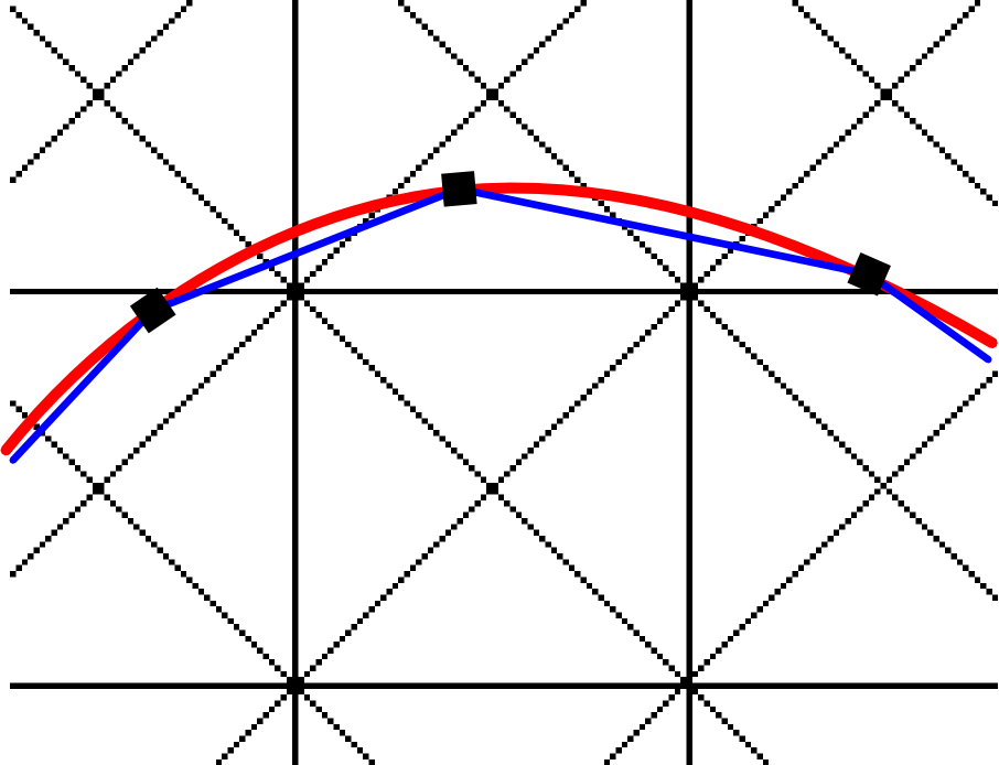
(a) Here we take an arbitrary interpolation of $\Gamma$. This does not have any relation to the triangulation $T_{h}$, so calculating integrals over $\Gamma_{\sigma}$ may be tricky.

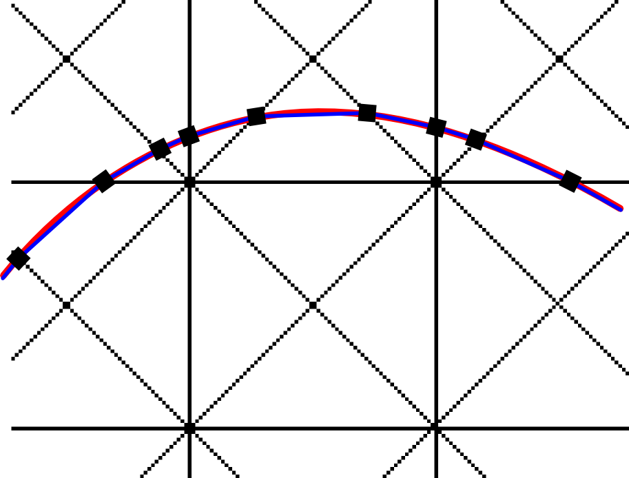
(b) Here we construct the interpolation of $\Gamma$ using the triangulation $T_{h}$; the beginning and end of segments of $\Gamma_{\sigma}$ are given by the points where $\Gamma$ intersects the edges of $T_{h}$. This makes calculating integrals over $\Gamma_{\sigma}$ easier.

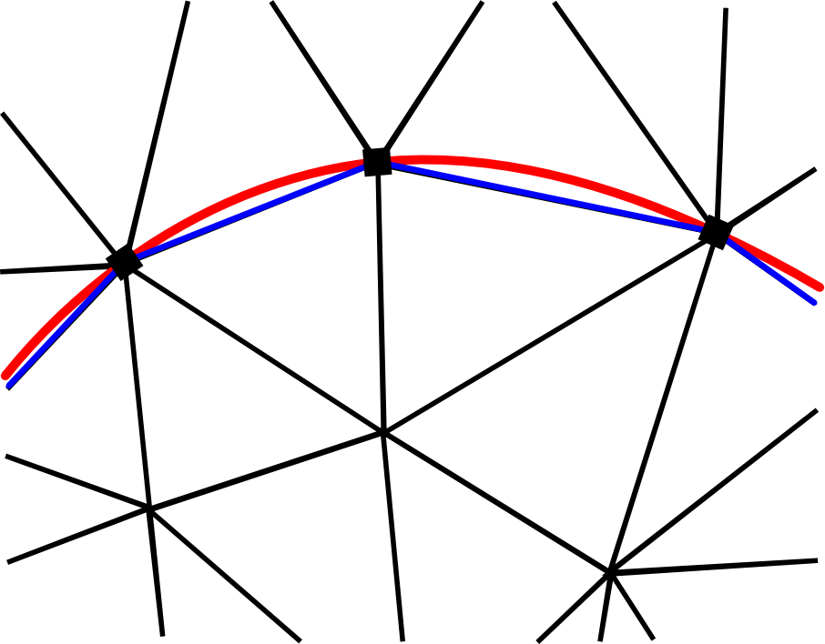
(c) Here $\Gamma_{\sigma}$ is chosen first then $T_{h}$ is constructed to contain the segments of $\Gamma_{\sigma}$ as edges. This leads to the easiest calculation of integrals over $\Gamma_{\sigma}$, but constructing $T_{h}$ may be hard.

Fig. 1: An illustration of different constructions of $T_{h}$ and polygonal $\Gamma_{\sigma}$ for $n=2$. The black lines mark the triangulation $T_{h}$, the red curve is $\Gamma$ and the blue curve is $\Gamma_{\sigma}$. The square markers indicate the beginning and end of segments of $\Gamma_{\sigma}$.

5.2 Link to optimal control at points

Method 2 can be thought of as using a quadrature to approximate Method 1. Note that

$$w_{\sigma}:=S_{h}\eta|_{\Gamma_{\sigma}}-I_{h}g_{\Gamma}\quad\forall\eta\in L^{2}(\Omega)$$

is piecewise linear on $\Gamma_{\sigma}$. Therefore

$$\|w_{\sigma}\|^{2}_{\Gamma_{\sigma}}=\int_{\Gamma_{\sigma}}w_{\sigma}^{2}\mathrm{d}A_{h}$$

corresponds to integrating a piecewise quadratic function on $\Gamma_{\sigma}$. This can be computed exactly with a weighted sum of point evaluations. In particular, Method 2 can be equivalently written as a discrete point control problem:

$$\min\frac{1}{2}\sum_{w\in I}\kappa_{\omega}\left|S_{h}\eta(\omega)-g_{\omega}\right|^{2}+\frac{\nu}{2}\|\eta\|^{2}_{L^{2}(\Omega)}\text{ over }\eta\in L^{2}(\Omega),$$

where $g_{\omega}:=g_{\Gamma}(\omega)$, the set $I$ contains points in $\Gamma$, and $\kappa_{\omega}$ are weights. If we construct a triangulation that contains $\Gamma_{\sigma}$ as edges (i.e. use approach $(c)$ in Figure 1) then $\left|I\right|=O(\frac{1}{h})$ and the $\kappa_{\omega}$ are $O(h)$.

As Theorem 16 holds using Method 2, we have provided an example of solutions to discrete point control problems that converge to the solution of a surface control problem.

Remark 21.

We could also consider a weighted fidelity term for the surface control problem i.e. replace the fidelity term in (1.1) by

$$\frac{1}{2}\int_{\Gamma}w(y-g_{\Gamma})^{2}\mathrm{d}A,$$

where $w\in L^{\infty}(\Omega)$ and $w\geq 0$. After the obvious modifications, all the results proved in this paper would still hold.

6 Numerical results

In this section we describe the numerical method we use to solve (4.7) and show that the error estimate from Theorem 16 for $n=2$ is observed in practice.

6.1 Numerical method

The numerical method is the same as the one described in [4] and [3] but for a discrete problem without a forcing term $f$ and the point evaluation term replaced by a surface integral term. If $u_{h}$ solves (4.7), then by substituting $u_{h}=\mathbb{P}_{[a,b]}(-\frac{1}{\nu}p_{h})$ we get that the state $y_{h}:=S_{h}u_{h}\in V_{h}$ and the adjoint variable $p_{h}\in V_{h}$ solve

$$\left(\begin{array}[]{c}a(y_{h},v_{h})-(-\frac{1}{\nu}p_{h}+(a+\frac{1}{\nu}p_{h})^{+}-(-\frac{1}{\nu}p_{h}-b)^{+},v_{h})\\ a(v_{h},p_{h})-m_{\sigma}(y_{h}|_{\Gamma_{\sigma}}-g_{\Gamma,\sigma},v_{h}|_{\Gamma_{\sigma}})\end{array}\right)=0\quad\forall v_{h}\in V_{h},$$ (6.1)

for all $v_{h},w_{h}\in V_{h}$. Here $v^{+}$ denotes the nonnegative part of $v$ i.e. $\max(0,v)$. Once this problem has been solved, the $u_{h}$ solving (4.7) can easily be determined from $p_{h}$ by setting $u_{h}=\mathbb{P}_{[a,b]}\big{(}-\frac{1}{\nu}p_{h}\big{)}$.

We use a semismooth Newton method to solve the above system, but we will not describe the algorithm in detail as it follows from only minor modifications to the one in [4] and [3]. We implemented the algorithm for $n=2$ in the Distributed and Unified Numerics Environment (DUNE) using DUNE-FEM (see [2, 1, 9]). This environment has the advantage that once an algorithm has been implemented, it is straightforward to change features of the implementation that would usually be fixed. For solving the linear systems for each iteration of the Newton method we used the biconjugate gradient stabilised method with an incomplete LU factorisation or Gauss-Seidel preconditioner. We do not implement the $n=3$ as this would be more complicated.

Depending on the example we are considering, we may either use Method 1 or Method 2 to choose $\Gamma_{\sigma}$, $m_{\sigma}$ and $g_{\Gamma,\sigma}$. When using Method 2 we will use the approach from Figure 1(c) and construct the triangulation $T_{h}$ from $\Gamma_{\sigma}$: We first find a polygonal curve $\Gamma_{\sigma}$ with segments of length $h$ (i.e. we take $\sigma=h$), and then use the program Triangle (see [22]) to construct a triangulation $T_{h}$ of size $h$ that contains the segments of $\Gamma_{\sigma}$ as edges.

6.2 Examples

In all our examples we will take $A=-\Delta$ and $\sigma=h$. We first solve two simple examples on a $\Gamma$ that is a straight line.

Example 22.

$\Omega=(0,1)^{2}$, $\Gamma=\{(0.25+0.5t,0.5):t\in(0,1)\}$, $g_{\Gamma}(x_{1},x_{2})=\sin(3\pi x_{1})$, $\nu=1e-2$, $b=-a=\infty$.

Example 23.

The same as Example 22 but with

$$g_{\Gamma}(x_{1},x_{2})=\begin{cases}1&x<0,\\ -1&x\geq 0\\ \end{cases}$$

and $b=-a=5$.

Example 22 has a smooth but nonconstant $g_{\Gamma}$ and no control constraints. Its solution can be seen in Figure 2. Example 23 has a discontinuous $g_{\Gamma}$ and active control constraints. Its solution can be seen in Figure 3. Even for these simple examples the exact solution is not known explicitly, so we compute $L^{2}(\Omega)$ errors against discrete solutions on fine triangulations to get approximate experimental orders of convergence (EOCs). In particular we use

$$\mathrm{EOC}_{h}=\frac{\log(\|\tilde{u}-u_{h/2}\|_{L^{2}(\Omega)}/\|\tilde{u}-u_{h}\|_{L^{2}(\Omega)})}{\log 2}$$

with $h_{\text{fine}}=0.00276214$, which corresponds to 263169 DOFs. The approximate EOCs for these examples are in Tables 6.2 and 3. They agree with the error estimate we proved in Theorem 16 for $n=2$. We do not verify this error estimate for examples with curved $\Gamma$: With our approach of constructing triangulations $T_{h}$ that coincide with $\Gamma_{\sigma}$, the resulting $T_{h}$ for a small $h$ will not in general be a refinement of a $T_{h}$ for a larger $h$. This makes it challenging to compute $L^{2}(\Omega)$ errors.

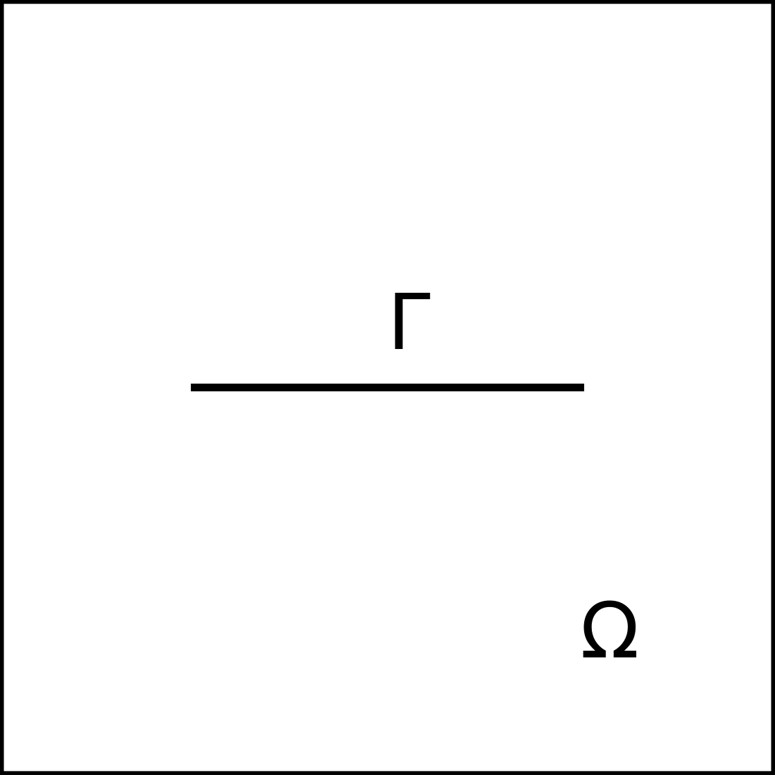
(a) Illustration of $\Gamma$.

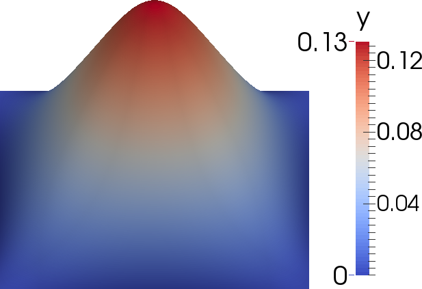
(b) Surface plot of $y_{h}$.

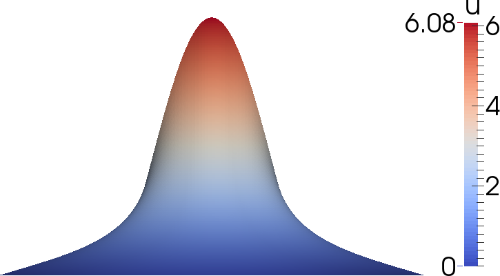
(c) Surface plot of $u_{h}=-\frac{1}{\nu}p_{h}$ with the $x_{1}$-axis at the bottom.

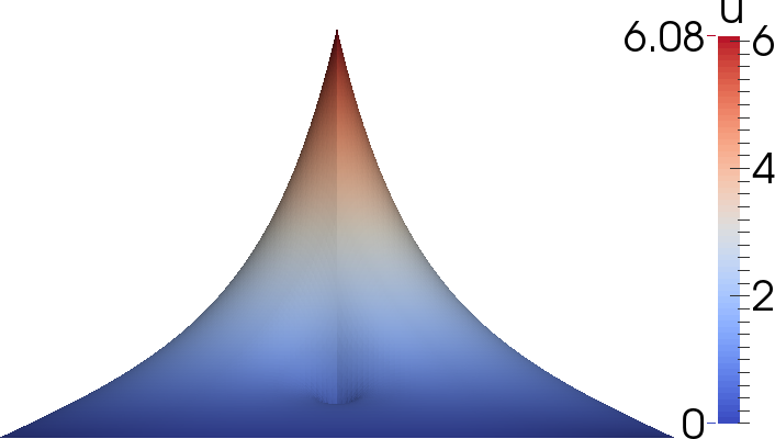
(d) Surface plot of $u_{h}=-\frac{1}{\nu}p_{h}$ with the $x_{2}$-axis at the bottom.

Fig. 2: The solution to Example 22. We use $\Gamma_{\sigma}$, $m_{\sigma}$ and $g_{\Gamma,\sigma}$ defined by Method 2, even though we do not need to approximate $\Gamma$, as interpolating $g_{\Gamma}$ simplifies the implementation.

(a) Illustration of $\Gamma$.

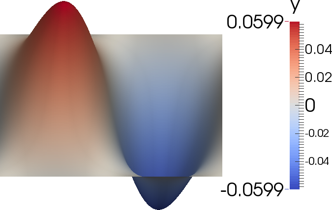
(b) Surface plot of $y_{h}$.

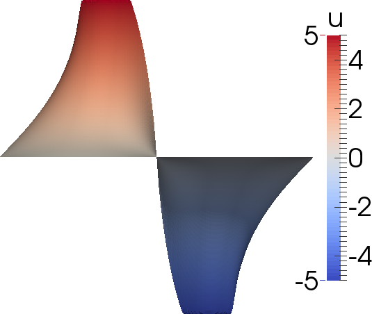
(c) Surface plot of $u_{h}=\mathbb{P}_{[a,b]}\big{(}-\frac{1}{\nu}p_{h}\big{)}$ with the $x_{1}$-axis at the bottom.

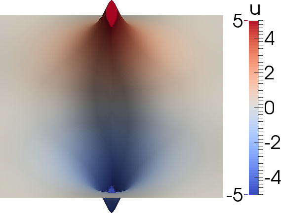
(d) Surface plot of $u_{h}=\mathbb{P}_{[a,b]}\big{(}-\frac{1}{\nu}p_{h}\big{)}$ with the $x_{2}$-axis at the bottom.

Fig. 3: The solution to Example 23. We use $\Gamma_{\sigma}$, $m_{\sigma}$ and $g_{\Gamma,\sigma}$ defined by Method 1, as it is easy to integrate discrete functions against $g_{\Gamma,\sigma}$ along $\Gamma$. The figure can be interpreted in the same way as Figure 2.

h	DoFs	$\|u_{h}-\tilde{u}\|_{\Omega}$	EoC
0.353553	25	0.92096	-
0.176777	81	0.413261	1.1561
0.0883883	289	0.193377	1.0956
0.0441942	1089	0.0967977	0.9984
0.0220971	4225	0.0482398	1.0047
0.0110485	16641	0.0235625	1.0337

Table 2: EOCs for Example 22 (which has no active control constraints).

$h$	# DoFs	$\|u-u_{h}\|_{L^{2}(\Omega)}$	$\text{EOC}_{h}$
0.353553	25	0.991883	0
0.176777	81	0.544039	0.86646341
0.0883883	289	0.292202	0.89674110
0.0441942	1089	0.146281	0.99822529
0.0220971	4225	0.0741029	0.98114049
0.0110485	16641	0.0363584	1.0272346

Table 3: EOCs for Example 23 (which has active control constraints).

In comparison to solutions of point control problems, the solutions of these line control examples appear to have bounded $p$ (and hence also $u$). An interesting feature of the solutions are the ridges in $p_{h}$ and $u_{h}$ along $\Gamma$. Observe that in the above examples $y_{h}|_{\Gamma}$ does not get close to $g_{\Gamma}$ because $\nu=1e-2$ is too large, especially when there are control constraints. In the next examples we take $\nu=1e-4$ and observe that we can get close agreement between $y_{h}|_{\Gamma}$ and $g_{\Gamma}$. In the remaining examples the only variable that will change is $\Gamma$.

Example 24.

$\Omega=(0,1)^{2}$,

$$\Gamma=\{(0.5+0.327t\sin t,0.5+0.327t\cos t):t\in(0,3.159)\},$$

(i.e. a spiral), $g_{\Gamma}=1$, $\nu=1e-4$, $b=-a=\infty$.

Example 25.

The same as Example 24 but with a multi-component $\Gamma$ having the spoke like structure marked by the black lines in Figure 6(c).

In Example 24 $\Gamma$ is curved. As described in Section 6, we first construct a $\Gamma_{\sigma}$ that interpolates $\Gamma$, then create a triangulation that coincides with $\Gamma_{\sigma}$. To illustrate this a possible (but coarse) triangulation for the spiral shaped $\Gamma$ from Example 24 is shown in Figure 4. In Example 25 the spoke like $\Gamma$ is formed from a $\Gamma$ consisting of multiple connected components; in particular, 6 open lines originating from the point $(0.5,0.5)$.

Solutions to Examples 24 and 25 can be seen in Figures 5 and 6. These were computed with $h=0.00292967$ and $\#\mathrm{DOFs}\approx 70000$. Observe that for this small value of $\nu=1e-4$, the values of $y_{h}|_{\Gamma}$ are close to $g_{\Gamma}=1$.

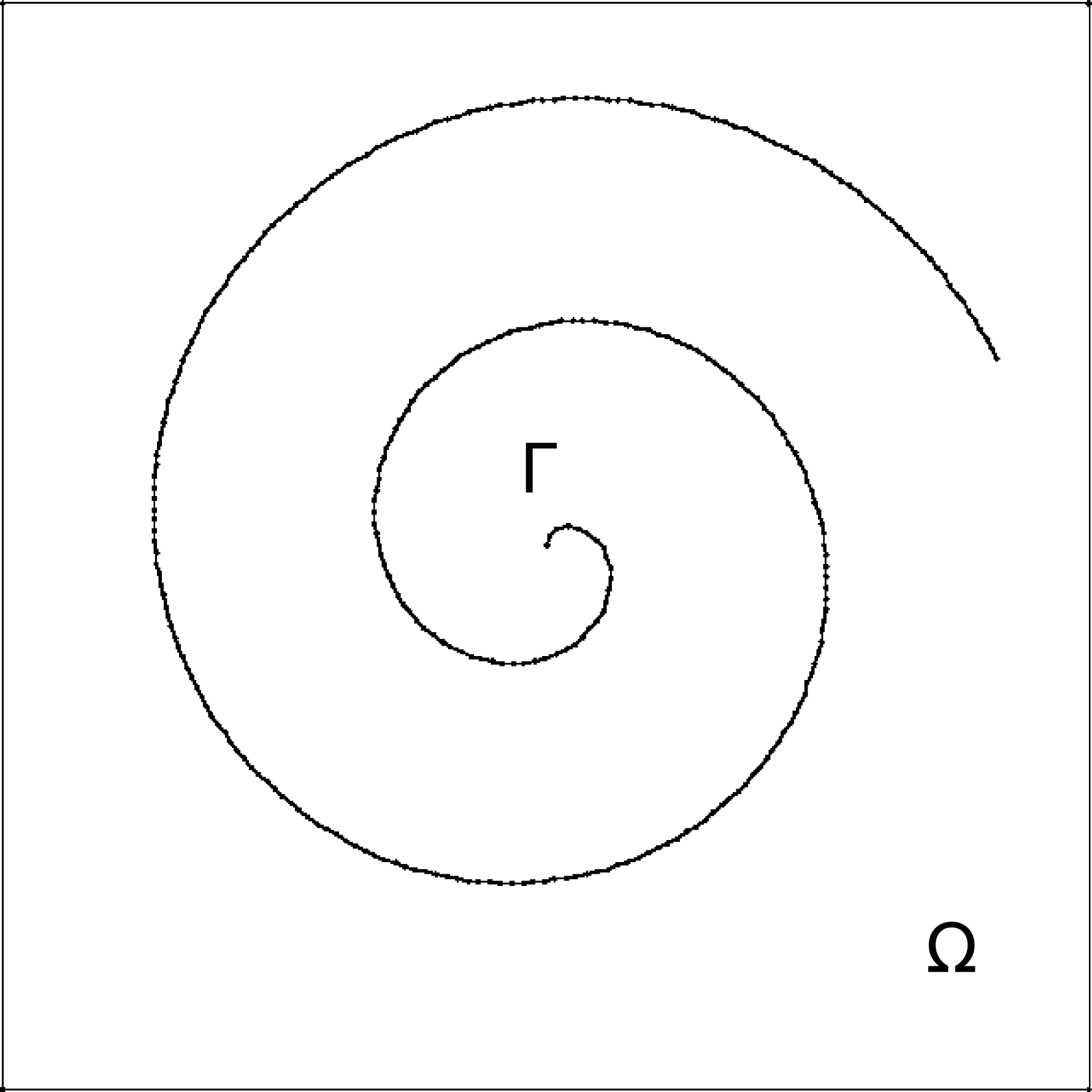
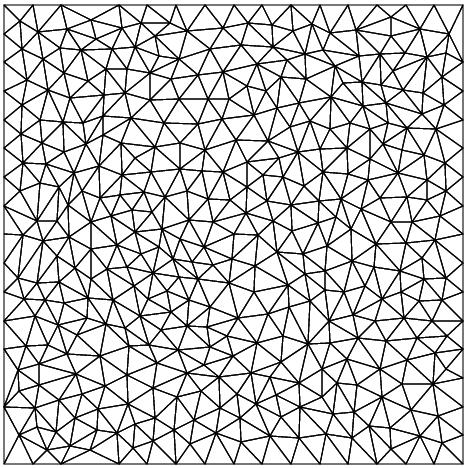
Fig. 4: $\Gamma$ as defined in Example 24 and a triangulation whose edges contain an interpolating polygonal approximation of it.

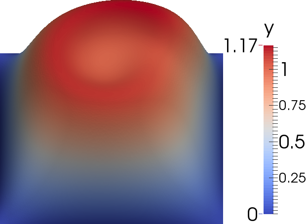
(a) Surface plot of $y_{h}$.

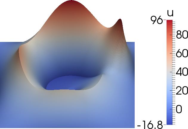
(b) Surface plot of $u_{h}=-\frac{1}{\nu}p_{h}$.

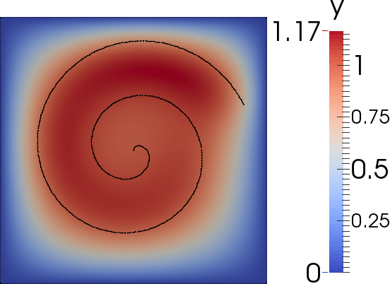
(c) Colour map of $y_{h}$.

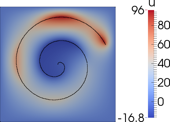
(d) Colour map of $u_{h}=-\frac{1}{\nu}p_{h}$.

Fig. 5: The solution to Example 24. We use $\Gamma_{\sigma}$, $m_{\sigma}$ and $g_{\Gamma,\sigma}$ defined by Method 2. The black curve is $\Gamma$.

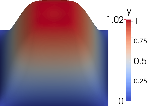
(a) Surface plot of $y_{h}$.

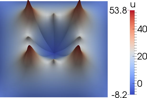
(b) Surface plot of $u_{h}=-\frac{1}{\nu}p_{h}$.

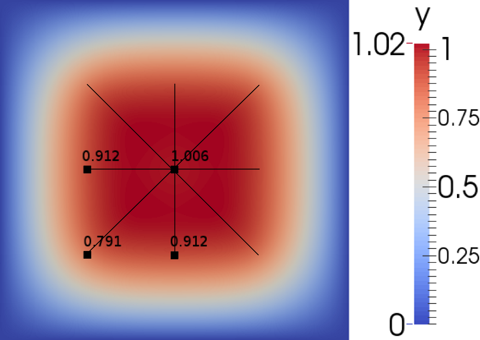
(c) Colour map of $y_{h}$.

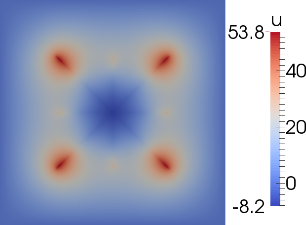
(d) Colour map of $u_{h}=-\frac{1}{\nu}p_{h}$.

Fig. 6: The solution to Example 25. We use $\Gamma_{\sigma}$, $m_{\sigma}$ and $g_{\Gamma,\sigma}$ defined by Method 1. The black curve is $\Gamma$ and the dots and numerical values indicate the value of $y_{h}$ at certain points on $\Gamma$. Not many points are included due to the symmetry of the solution.

6.3 Comparison to optimal control at points

To finish we compare the solution of the line problem from Example 24 (shown in Figure 5) with the following point control problem.

Example 26.

$\Omega=(0,1)^{2}$,

$$\Gamma=\{(0.5+0.327t\sin t,0.5+0.327t\cos t):t\in(0,3.159)\},$$

(i.e. a spiral), $I$ is a set of $41$ evenly spaced points along $\Gamma$, $g_{\omega}=1$ for all $\omega\in I$, $\nu=1e-4$, $b=-a=\infty$.

The theory for such problems is covered in [4]. Note that we take the same parameter values as for the line problem except instead of a prescribed function $g_{\Gamma}=1$, we have prescribed values of $g_{\omega}=1$ at points along $\Gamma$. The solution of this problem can be seen in Figure 7.

We see in Figure 7(c) that the point problem gets $y_{h}|_{\Gamma}$ closer to $1$ than the line problem. However this is at the cost of $\|u_{h}\|_{L^{2}(\Omega)}=36.5414$ for the point problem compared to $\|u_{h}\|_{L^{2}(\Omega)}=28.0718$ for the line problem, and a what appears to be unbounded $\|u\|_{\infty}$.

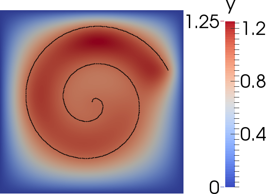
(a) Colour map of $y_{h}$. The black line is the curve $\Gamma$ along which the points are evenly distributed.

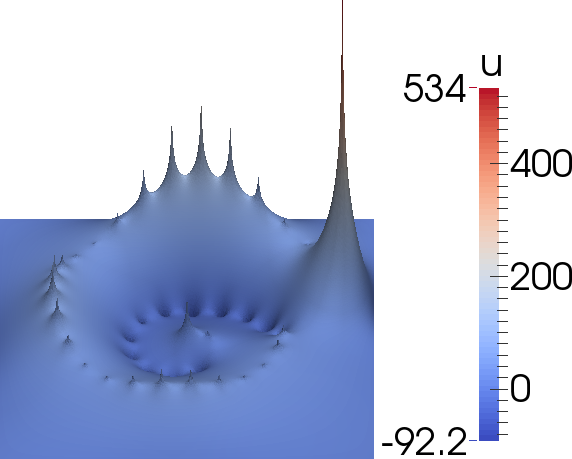
(b) Surface plot of $u_{h}=-\frac{1}{\nu}p_{h}$.

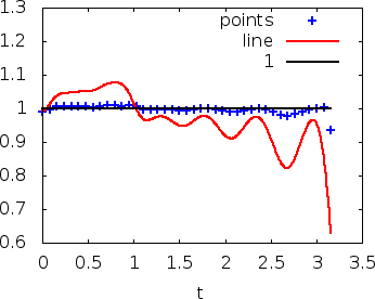
(c) Comparison of $y_{h}$ from this point control problem evaluated on $I$, against $y_{h}$ from the line control problem of Example 24 (shown in Figure 5) evaluated along $\Gamma$ starting from the centre.

Fig. 7: The solution of Example 26. Compare to Figure 5.

Recall our observation from Section 5.2 that solutions of appropriately weighted discrete point control problems converge to the solution of a surface control problem. The points and weights we mentioned arose from Method 2. A simpler approach, which nevertheless works well in practice, is to choose an arbitrary triangulation of size $h$, then take $\lceil\frac{\left|\Gamma\right|}{h}\rceil$ (where $\lceil\cdot\rceil$ denotes the ceiling function) evenly spaced points along $\Gamma$ and weight them by $h$. Given an arclength parameterisation of $\Gamma$, it is straightforward to adapt the implementation in [4] to do this.

The solution to the point control problem resulting from this approach is almost indistinguishable to the solution of the line control problem using Method 2, so we do not include it in a figure. A minor difference is that the ridge in $u_{h}$ is slightly jagged, as the edges of the triangulation do not necessarily align with it, but as $h$ is reduced this effect disappears.

References

- [1] P. Bastian, M. Blatt, A. Dedner, C. Engwer, R. Klöfkorn, R. Kornhuber, M. Ohlberger, and O. Sander, A generic grid interface for parallel and adaptive scientific somputing. Part II: Implementation and tests in DUNE, Computing, 82 (2008), pp. 121–138.
- [2] P. Bastian, M. Blatt, A. Dedner, C. Engwer, R. Klöfkorn, M. Ohlberger, and O. Sander, A generic grid interface for parallel and adaptive scientific computing. Part I: Abstract framework, Computing, 82 (2008), pp. 103–119.
- [3] C. Brett, Optimal control and inverse problems involving point and line functionals and inequality constraints, PhD thesis, University of Warwick, 2014.
- [4] C. Brett, A. S. Dedner, and C. M. Elliott, Optimal control of elliptic PDEs at points (preprint), (2014).
- [5] C. Brett, C. M. Elliott, M. Hintermüller, and C. Löbhard, Mesh adaptivity in optimal control of elliptic variational inequalities with point-tracking of the state, Interfaces and Free Boundaries (submitted), (2013).
- [6] E. Casas, C. Clason, and K. Kunisch, Approximation of elliptic control problems in measure spaces with sparse solutions, SIAM Journal on Control and Optimization, 50 (2012), pp. 1735–1752.
- [7] P. G. Ciarlet, The finite element method for elliptic problems, Studies in Mathematics and its Applications, North-Holland, 1978.
- [8] K. Deckelnick and M. Hinze, Convergence of a finite element approximation to a state-constrained elliptic control problem, SIAM Journal on Numerical Analysis, 45 (2007), pp. 1937–1953.
- [9] A. Dedner, R. Klöfkorn, M. Nolte, and M. Ohlberger, A generic interface for parallel and adaptive scientific computing: abstraction principles and the DUNE-FEM module, Computing, 90 (2010), pp. 165–196.
- [10] A. Demlow, Higher-order finite element methods and pointwise error estimates for elliptic problems on surfaces, SIAM Journal on Numerical Analysis, 47 (2009), pp. 805–827.
- [11] G. Dziuk, Finite elements for the Beltrami operator on arbitrary surfaces, in Partial Differential Equations and Calculus of Variations, Stefan Hildebrandt and Rolf Leis, eds., Lecture Notes in Mathematics, Springer, 1988, pp. 142–155.
- [12] G. Dziuk and C. M. Elliott, Finite element methods for surface PDEs, Acta Numerica, 22 (2013), pp. 289–396.
- [13] L. Evans, Partial Differential Equations, vol. 19 of Graduate Studies in Mathematics, American Mathematical Society, 2nd ed., 2010.
- [14] D. Gilbarg and N. S. Trudinger, Elliptic partial differential equations of second order, vol. 224 of Classics in Mathematics, Springer, 2001.
- [15] W. Gong, G. Wang, and N. Yan, Approximations of elliptic optimal control problems with controls acting on a lower dimensional manifold, SIAM Journal on Control and Optimization, 52 (2014), pp. 2008–2035.
- [16] P. Grisvard, Elliptic problems in nonsmooth domains, vol. 24 of Monographs and Studies in Mathematics, Pitman Advanced Publishing Program, 1985.
- [17] M. Hinze, A variational discretization concept in control constrained optimization: The linear-quadratic case, Computational Optimization and Applications, 30 (2005), pp. 45–61.
- [18] M. Hinze, R. Pinnau, and M. Ulbrich, Optimization with PDE constraints, vol. 23 of Mathematical Modelling: Theory and Applications, Springer, 2009.
- [19] D. Leykekhman, D. Meidner, and B. Vexler, Optimal error estimates for finite element discretization of elliptic optimal control problems with finitely many pointwise state constraints, Computational Optimization and Applications, 55 (2013), pp. 769–802.
- [20] C. B. Morrey Jr., Multiple integrals in the calculus of variations, vol. 130 of Grundlehren der mathematischen Wissenschaften, Springer, 1966.
- [21] K. Pieper and B. Vexler, A priori error analysis for discretization of sparse elliptic optimal control problems in measure space, SIAM Journal on Control and Optimization, 51 (2013), pp. 2788–2808.
- [22] J. R. Shewchuk, Triangle web page (http://www.cs.cmu.edu/quake/triangle.html).
- [23] F. Tröltzsch, Optimal control of partial differential equations: Theory, methods and applications, vol. 112 of Graduate Studies in Mathematics, American Mathematical Society, 2010.
- [24] A. Unger and F. Tröltzsch, Fast solution of optimal control problems in the selective cooling of steel, ZAMM ‐Journal of Applied Mathematics and Mechanics, 81 (2001), pp. 447–456.
- [25] W. P. Ziemer, Weakly differentiable functions: Sobolev spaces and functions of bounded variation, vol. 120 of Graduate Texts in Mathematics, 1989.