Modelling of dependence in high-dimensional financial time series by cluster-derived canonical vines

Abstract

We extend existing models in the financial literature by introducing a cluster-derived canonical vine (CDCV) copula model for capturing high dimensional dependence between financial time series. This model utilises a simplified market-sector vine copula framework similar to those introduced by Heinen and Valdesogo (2008) and Brechmann and Czado (2013), which can be applied by conditioning asset time series on a market-sector hierarchy of indexes. While this has been shown by the aforementioned authors to control the excessive parameterisation of vine copulas in high dimensions, their models have relied on the provision of externally sourced market and sector indexes, limiting their wider applicability due to the imposition of restrictions on the number and composition of such sectors. By implementing the CDCV model, we demonstrate that such reliance on external indexes is redundant as we can achieve equivalent or improved performance by deriving a hierarchy of indexes directly from a clustering of the asset time series, thus abstracting the modelling process from the underlying data.

1 Introduction

This paper introduces a new model for capturing high dimensional dependence which we term the cluster-derived canonical vine (CDCV) copula model, with a direct application to the practical modelling of large portfolios of financial assets. Whilst the implementation of such advanced dependence models is infrequent in the financial industry, more basic dependence models are none-the-less heavily utilised. The ability to describe the behaviour of a given financial variable in terms of other financial variables enables us to both make use of the proliferation of data that is available in the market and to derive proxies for financial variables when data is not available. Moreover, when we consider the behaviour of financial variables such as basket options, equity portfolios or complex credit products that are directly dependent on their constituent variables, we clearly require a method of capturing not just the marginal behaviour of the constituents, but also the evolution of the dependence structure between the constituents.

One of the more basic approaches to capturing such multivariate dependence is the multivariate copula. First introduced by [21] as a statistical tool, the copula decomposes a given multivariate distribution into a dependence structure and a set of marginal distributions. Multivariate copulas have arguably become an industry standard for capturing dependence despite the negative press that the Gaussian copula based Default Correlation model of [16] garnered in the wake of the 2008 financial downturn (see [19]). Due to its ability to capture stylised features of financial variables such as fat tails, the Student’s-t copula in particular is commonly utilised. However, despite their widespread use, such parametric multivariate copulas still present a level of inflexibility in that they are essentially “one-size-fits-all” and may not fully capture the nuances of a given multivariate dependence structure.

This inflexibility has been addressed in the academic sphere by the introduction of highly parametrised vine copulas (see [10, 3]), which decompose the copula dependence structure into a collection of trees containing bivariate copulas. Vine copulas enable the modeller to select different bivariate copulas to represent the dependence between different pairs of variables. This has the obvious advantage of more accurately capturing complex and heterogeneous dependence structures, and provides access to the much broader range of bivariate copulas that exist for capturing features such as tail dependence. Recent growth in the vine copula literature can be traced to the paper “Pair-Copula Constructions of Multiple Dependence” [1] which built upon the work of [10] and [3] by firstly bringing their introduction of the vine copula to the forefront of the literature and secondly, by illustrating how a vine copula model could be constructed and fitted to data, given a set of marginal distributions and a cascade of conditional pair copulas. However, the practical application of vine copulas has been limited to relatively low dimensional problems due to the need to fit the parameters of as many as $m(m-1)/2$ bivariate copulas in an $m$-dimensional model. Even with the latest computational technology the model fitting process quickly becomes infeasible for these models in higher dimensions.

To overcome this curse of dimensionality, a number of techniques have been proposed. The most straightforward approach is that of vine simplification or truncation, as described by [9], [15] and [5], among others. This approach essentially approximates the vine copula, by taking advantage of the de minimus contribution of later vine trees to the modelled dependence structure. Secondly, the class of Market Sector Vine Copula models (such as the CAVA model of [9] and the RVMS model of [5]) aims to reduce the implementation cost of vine copulas significantly via the introduction of a pre-existing market-sector index hierarchy (such as the S&P500) upon which elements may be conditioned given simplifying assumptions regarding inter-sector dependence. By conditioning asset time series on these index time series, such models have enabled the flexibility of vine copulas to be applied to portfolios of much higher dimensions by limiting the number of trees that need to be fitted to achieve a fixed level of model accuracy. Finally, recent research by [4, 6, 13, 18, 11] has sought to develop hierarchical vine models that are not reliant on externally sourced hierarchies, in a similar spirit to our own research. For example, [6] use factor analysis to develop latent factors upon which all elements are then conditioned before utilising a truncated R-Vine copula to capture the remaining idiosyncratic dependence between elements. The approach of [18] similarly uses factor analysis to derive the root nodes of C-Vine copula trees. The authors do not seek to segment or cluster the population of elements in the style of market sector vine copulas, but rather to utilse underlying factors common to all elements. More recently, [13] and [11] have proposed and then defined the Bi-factor copula model which can be used when we have many variables which are divided into groups, making the natural step of combining the market-sector hierarchy of [9, 5] with the derivation of latent factors for both the market and the sector groups.

Our research and development of the CDCV model is also motivated by the Market Sector Vine Copula models of [9] and [5], which focus on illustrative examples utilising specific externally-introduced market-sector hierarchies. It is not immediately clear to what extent these models can be applied to other data sets; whether the model performance varies based on the external indexes used; whether the size, number or composition of the sectors impacts model performance; whether dependence structures and model performance vary through time, or even whether it is always appropriate or possible to use such external indexes. It is this class of models that we extend via the introduction of the CDCV model, which mirrors the recently proposed Bi-factor copula model of [11] by replacing the externally sourced S&P500 and Euro Stoxx 50 indexes of the CAVA and RVMS models respectively with derived variables. An additional feature of the CDCV model is that we can apply this market-sector hierarchical structure to any data set, irrespective of whether the data is already grouped into obvious segments or clusters. We do so by applying clustering and index construction methodologies to the data, which allows the resulting market-cluster hierarchical structure to vary in time and allows variables to move between clusters. As such, the derived cluster indexes of the CDCV model represent discrete dynamic clusters of elements that may be considered analogous to sub-portfolios or trading books in a financial context. The CDCV approach is thus additive in principle, in that as larger pools of underlying elements are considered, the derived indexes can be combined and re-used as necessary providing consistent index construction methodologies are used. This leads us to question the practical limitations of such factor-copula models, which we begin to address in Section 3.

In the following section, we formally introduce the CDCV model, outlining the fundamental clustering and index creation steps while referring the reader to the Appendix for details of the model fitting process, performed using the Inference Functions for Margins (IFM) method of [12]. In Section 3 we provide an empirical analysis of the CDCV model’s performance against an equivalent (fixed hierarchy) market sector model of the CAVA-type proposed by [9]. In this section we demonstrate that such models need not rely on an external hierarchy and that equivalent or better performance can be obtained by conditioning assets on indexes derived directly from the underlying data. We also extend the analysis of [9, 5, 11, 13] by demonstrating that the composition of Market Sector Vine Copula models has a material impact on model performance and that model performance is time-dependent. Finally, we conclude and discuss areas for further research in Section 4.

2 The CDCV Model

We now formally introduce in detail the proposed cluster-derived canonical vine (CDCV) copula model, depicted in Figure 1. By deriving indexes rather than utilising externally sourced indexes, we mirror the Bi-factor copula model approach of [11] but extend the model’s applicability to arbitrary data sets via additional clustering and index derivation steps. This extension is important in practice as we may find that there are many natural groupings of the variables and it may not be practical to fit all of them. We perform conditioning as part of a C-vine fitting process upon indexes derived from these asset clusters. We allow these clusters to evolve through time subject to a set of configurable clustering rules (see Appendices A.1 and A.2) and using a general clustering algorithm (see Appendix A.3). As such, we may draw a parallel to the management of portfolios in a financial setting.

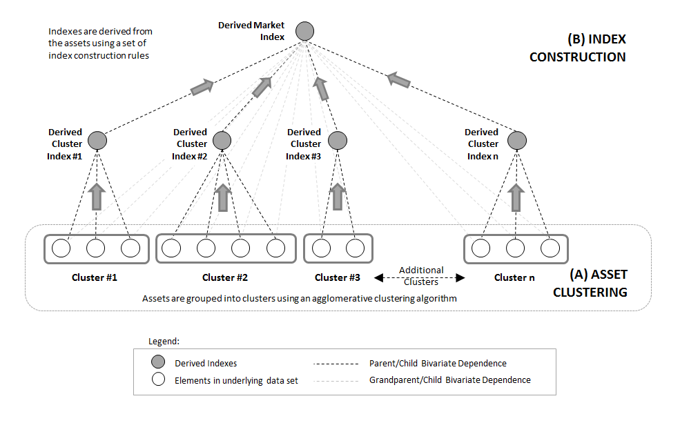
Figure 1: Diagrammatic representation of the CDCV model’s derived hierarchical structure, obtained by grouping assets into $n$ clusters and then constructing indexes for each. The market index can then be constructed from the cluster indexes or directly from all assets.

In order to implement this model we face two primary challenges; firstly how to group or cluster the assets to maximise the dependence captured by the model, and secondly how to use these groupings to derive optimal sector and market indexes. Figure 1 illustrates these challenges in the context of our proposed CDCV model, for which we will utilise the same hierarchical C-Vine decomposition as the CAVA model of [9] to enable us to compare performance against that model in Section 3. This decomposition can be defined in this more general setting as

$$f_{CDCV}\left(r_{M},\,r_{S_{1}},...,\,r_{S_{E}},\,r_{1}^{S_{1}},...,\,r_{Z^{1}}^{S_{1}},......,\,r_{1}^{S_{E}},...,\,r_{Z^{E}}^{S_{E}}\right)=\bar{f}\cdot\bar{c}_{M,S}\cdot\bar{c}_{M,A}\cdot\bar{c}_{S,A\mid M}\cdot\bar{c}_{A}\,,$$ (1)

where $r_{M}$ is the market index return, $r_{S_{i}}$ are the $1\leq i\leq E$ cluster index returns, and $r_{j}^{S_{i}}$ are the $1\leq j\leq Z_{i}$ asset returns associated with cluster $i$. The marginals appear in

$$\begin{array}[]{ccl}\bar{f}&=&f\left(r_{M}\right)\cdot f\left(r_{S_{1}}\right)\cdot...\cdot f\left(r_{S_{E}}\right)\cdot\left[f\left(r_{1}^{S_{1}}\right)\cdot...\cdot f\left(r_{Z_{1}}^{S_{1}}\right)\right]\cdot...\cdot\left[f\left(r_{1}^{S_{E}}\right)\cdot...\cdot f\left(r_{Z_{E}}^{S_{E}}\right)\right]\end{array}.$$ (2)

The unconditional copulas between the market index and the sector indexes are given by

$$\begin{array}[]{ccl}\bar{c}_{M,S}&=&c_{r_{M},r_{S_{1}}}\left[{\scriptstyle F\left(r_{M}\right),F\left(r_{S_{1}}\right)}\right]\cdot...\cdot c_{r_{M},r_{S_{E}}}\left[{\scriptstyle F\left(r_{M}\right),F\left(r_{S_{E}}\right)}\right]\end{array}$$ (3)

and the remaining unconditional copulas between the market index and the assets are

$$\begin{array}[]{cccl}\bar{c}_{M,A}&=&\left[c_{r_{M},r_{1}^{S_{1}}}\left[{\scriptstyle F\left(r_{M}\right),F\left(r_{1}^{S_{1}}\right)}\right]\cdot...\cdot c_{r_{M},r_{Z_{1}}^{S_{1}}}\left[{\scriptstyle F\left(r_{M}\right),F\left(r_{Z_{1}}^{S_{1}}\right)}\right]\right]&\cdot...\cdot\\ &&\left[c_{r_{M},r_{1}^{S_{E}}}\left[{\scriptstyle F\left(r_{M}\right),F\left(r_{1}^{S_{E}}\right)}\right]\cdot...\cdot c_{r_{M},r_{Z_{E}}^{S_{E}}}\left[{\scriptstyle F\left(r_{M}\right),F\left(r_{Z_{E}}^{S_{E}}\right)}\right]\right]&\,,\end{array}$$ (4)

where $c_{r_{M},r_{S_{j}}}$ denotes the bivariate copula between the market index and the sector $j$ index. The CDCV model then captures the dependence between each asset and its respective sector index (conditioned upon the market index) via conditional copulas, as represented by the $\bar{c}_{S,A\mid M}$ term in (1). In the context of a C-Vine copula, the market index can thus be considered to be the root node of the first tree, while the subsequent trees select the sector indexes as their nodes. The ordering of these subsequent trees is arbitrary due to the assumption of conditional independence between cluster indexes and between cluster indexes and assets from other clusters. The $\bar{c}_{S,A\mid M}$ term is given as

$$\begin{array}[]{ccl}\bar{c}_{S,A\mid M}&=&\left[c_{r_{S_{1}},r_{1}^{S_{1}}\mid r_{M}}\left[{\scriptstyle F\left(r_{S_{1}}\mid r_{M}\right),F\left(r_{1}^{S_{1}}\mid r_{M}\right)}\right]\cdot...\cdot c_{r_{S_{1}},r_{Z_{1}}^{S_{1}}\mid r_{M}}\left[{\scriptstyle F\left(r_{S_{1}}\mid r_{M}\right),F\left(r_{Z_{1}}^{S_{1}}\mid r_{M}\right)}\right]\right]\cdot...\cdot\\ &&\left[c_{r_{S_{E}},r_{1}^{S_{E}}\mid r_{M}}\left[{\scriptstyle F\left(r_{S_{E}}\mid r_{M}\right),F\left(r_{1}^{S_{E}}\mid r_{M}\right)}\right]\cdot...\cdot c_{r_{S_{E}},r_{Z_{E}}^{S_{E}}\mid r_{M}}\left[{\scriptstyle F\left(r_{S_{E}}\mid r_{M}\right),F\left(r_{Z_{E}}^{S_{E}}\mid r_{M}\right)}\right]\right]\,,\end{array}$$ (5)

where $c_{r_{S_{j}},r_{i}^{S_{j}}\mid r_{M}}$ is the bivariate copula between sector $j$ and asset $i$ within that sector, conditioned on the market index. Finally, the CDCV model captures any remaining idiosyncratic dependence with a multivariate copula, utilising the technique of Joint Simplification (see [9]), where a multivariate copula is applied between all assets, each conditioned on the market index and on their associated sector index. This is represented in the decomposition by the $\bar{c}_{A}$ term, given as

$$\begin{array}[]{ccl}\bar{c}_{A}&=&c_{r_{1}^{S_{1}}...r_{Z^{1}}^{S_{1}}......r_{1}^{S_{E}}...r_{Z^{E}}^{S_{E}}\mid r_{M},r_{S_{1}},...,r_{S_{E}}}\\ &&\left[{\scriptstyle F\left(r_{1}^{S_{1}}\mid r_{S_{1}},\,r_{M}\right),...,F\left(r_{Z_{1}}^{S_{1}}\mid r_{S_{1}},\,r_{M}\right),...,...,F\left(r_{1}^{S_{E}}\mid r_{S_{E}},\,r_{M}\right),...,F\left(r_{Z_{E}}^{S_{E}}\mid r_{S_{E}},\,r_{M}\right)}\right]\,.\end{array}$$ (6)

While we have chosen to develop the CDCV model using the more standardised C-Vine specification used by the CAVA model of [9], a secondary step (not taken here) would be to assess the relative impact of our findings when applied to the more generalised R-Vine modelling structure, as utilised by [6].

2.1 Dynamically Grouping Assets into Clusters

As we choose to implement the same hierarchical C-Vine structure as the CAVA model of [9], we are interested in constructing clusters that minimise the dependence between assets in different clusters. While further work can be performed in this area to develop algorithms that achieve such optimal clusterings and thus capture the maximum possible dependence between assets, we will demonstrate that even a heuristic approach to selecting clusters can result in an improvement upon the existing sector-based approach of [9]. For the purposes of our analysis we will consider only agglomerative clustering methods, as visualised in Figure 2, which seek to iteratively group assets until some predetermined condition is met. These methods are less computationally intensive than divisive clustering methods which start from one super-set cluster and iteratively bifurcate the population(s) in each cluster. To develop clusters, we calculate dissimilarity metrics for each pair of elements at each iterative step in the process, as defined in Appendix A.1. We then apply a clustering rule, known as a linkage criterion, at each step to select which elements to join together into a cluster. Examples of common linkage criteria are given in Appendix A.2. Newly formed clusters then become elements in the next step and may be selected for joining. To perform this repeated joining of assets and clusters we may use a clustering algorithm as provided in Appendix A.3. Such an algorithm can then be controlled by the introduction of configurable parameters into the algorithm or rule itself; for example, to ensure a minimum cluster size, a fixed or varying number of clusters, and so on.

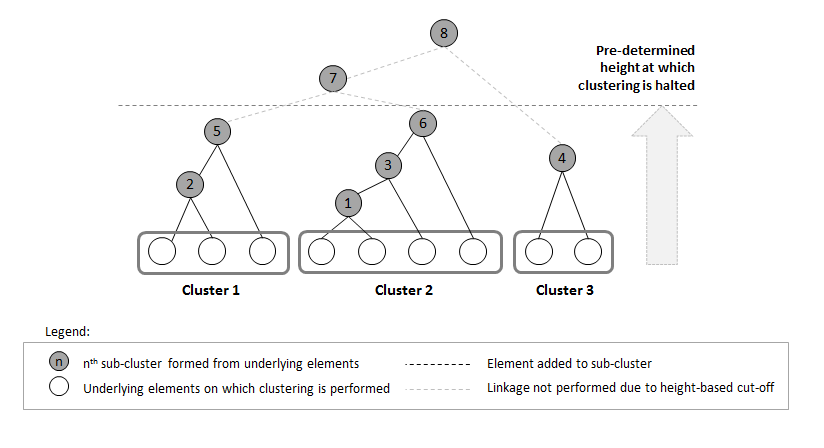
Figure 2: Diagrammatic representation of an agglomerative clustering approach for 9 assets subject to a height-based cut-off rule.

While the Euclidean distance is probably the most commonly used distance metric in the clustering literature (see [20, 8, 4] for an overview), we are more inclined to use rank correlation measures for this task as we are looking to group time series data that demonstrate the most dependence. In terms of the linkage criterion that we employ, the choice is largely driven by the type of clusters we are looking to produce. For example, the Average Linkage Criterion tends to join clusters with small within-cluster variances and also tends to be less affected by extreme values than many other methods. Alternatively, the Complete Linkage Criterion can be significantly impacted by moderately outlying values and is biased toward producing compact clusters of approximately equal radius. In our analysis of the CDCV model we will primarily choose to use an Adapted Single Linkage Criterion that we have introduced, incorporating some additional rules not included in the generic agglomerative clustering algorithm given in Appendix A.3. This criterion is similar to the standard Single Linkage Criterion, but it additionally limits the size of any given cluster to a parametrised maximum number of elements, limits the total number of clusters to a parametrised maximum value and ignores potential joins where both elements are already non-singleton clusters. This final restriction is implemented to avoid chaining, which can be an issue with Single Linkage algorithms, where each link covers a short distance but the most dissimilar elements in a cluster may end up quite distant from each other. To this extent, we can think of linkage criteria as not only a rule for deciding which clusters to merge, but also as a means for introducing additional conditions that provide greater control over the size, shape and composition of the resulting clusters. While the dynamic clustering approach of the CDCV model is clearly very intuitive, time-varying and a conceptual improvement over the fixed sector clustering methods, it should be noted that a further area for research remains to develop optimised clustering methods.

2.2 Deriving Hierarchical Indexes from the Assets

The assets that the CDCV model clusters into a particular grouping in a given time step may not be immediately representable by an existing index. We thus make use of a general index derivation methodology, illustrated in Figure 3, from which we may construct index(es) for each cluster to be used as latent variables in our model. While there are many possible methods by which we may derive these latent variables on which we will condition the assets, we will prefer methods that provide relatively stable cluster indexes through time.

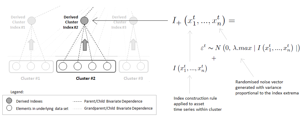
Figure 3: Diagrammatic representation of the methodology by which cluster indexes are derived in the CDCV model. A market index may then be derived either directly from the cluster indexes or directly from the set of all assets.

We outline in Appendix A.4 a number of basic but commonly used index construction rules (denoted $I\left(\cdot\right)$) that are used in the financial industry, and combine these with a normally distributed random variable “noise” vector given by

$$\varepsilon^{t}\thicksim N\left(0,\,\lambda\cdot\max\mid I\left(x_{1}^{t},...,x_{n}^{t}\right)\mid\right)\,,$$ (7)

where $\Upsilon=\frac{1}{\lambda}$ is a noise parameter that we use to adjust the scale of the perturbations to be introduced. This enables us to define our noise-adjusted index in each time step as

$$I_{+}\left(x_{1}^{t},...,x_{n}^{t}\right)=I\left(x_{1}^{t},...,x_{n}^{t}\right)+\varepsilon^{t}\,.$$ (8)

This noise term remediates an issue that arises from the process of constructing indexes directly from a small number of asset time series and then conditioning those time series on the resultant index. When cluster sizes are small, we may end up introducing artificially high levels of negative rank correlation into our model due to the index representing too perfectly a median path between two asset time series. As we will show in Section 3, this noise term is sufficient to dampen the negative rank correlations generated, while still capturing efficiently the positive dependence in the underlying asset time series data. While the optimisation of such index constructions is another area for further research, we will demonstrate in Section 3 that with only minimal attention to this problem we are able to construct sufficiently good indexes to obtain model fitting results that outperform an equivalent model utilising the CAVA model’s structure.

2.3 Implementing the CDCV Model

To implement the CDCV model as defined in this paper we have built up a modelling structure and test framework using the statistical programming language R. We have updated the algorithms described by [9] to provide Inference Functions for Margins (see [12]) model fitting and simulation algorithms for the CDCV model, which we provide in Appendix A.7 and A.8. In these algorithms we choose between Normal, Student’s-t and Skew Student’s-t marginal distributions using the Akaike Information Criterion (AIC, as per [2]), to ensure that we can capture characteristics of financial asset return time series such as excess skew and kurtosis. We also restrict ourselves to homoscedastic marginal distributions, in line with [17] who observe that the introduction of GARCH-type marginals had no noticeable impact on the results of their vine-copula focused portfolio optimisation analysis. Once we have fitted the marginal distributions, we transform the marginal data to the unit hypercube. For each bivariate combination of asset plus market index, we then maximise the bivariate log-likelihood of selected bivariate copula families, given in generality by [7] as

$$l(\Theta;\,x_{1},x_{2})=\overset{m}{\underset{i=1}{\sum}}\log\,\bar{C}_{\Theta}\left(F_{1}\left(x_{i,1}\right),F_{2}\left(x_{i,2}\right)\right)-\overset{m}{\underset{i=1}{\sum}}\overset{2}{\underset{j=1}{\sum}}\log\,f_{j}\left(x_{i,j}\right)\,,$$ (9)

where $\bar{C}_{\Theta}$ is the copula density defined for each trialled copula type. The set of marginal distributions is

$$\hat{\Omega}=\left\{F_{1}\left(x_{1};\,\hat{z}_{1}\right),F_{2}\left(x_{2};\,\hat{z}_{2}\right),...,F_{m}\left(x_{m};\,\hat{z}_{m}\right)\right\}\,,$$ (10)

and the resultant set of estimated marginal densities is

$$\hat{\Psi}=\left\{f_{1}\left(x_{1};\,\hat{z}_{1}\right),f_{2}\left(x_{2};\,\hat{z}_{2}\right),...,f_{n}\left(x_{m};\,\hat{z}_{m}\right)\right\}\,,$$ (11)

where $\hat{z}=\left\{\hat{z}_{1},...,\hat{z}_{m}\right\}$ is the set of estimated marginal parameters. Note that the second term of (9) does not depend on the copula parameter(s), and thus for the IFM approach we need only maximise the first term. The resulting log-likelihoods for the Gaussian, Student’s-t, Clayton and Frank copula families enable selection of the best fitting bivariate copula, again by AIC. However, model-fitting a C-Vine copula also requires us to apply an $h$-function (13) after each bivariate copula in the vine is fitted, in order to transform the sample data used to fit the copula into sample data which is additionally conditioned on the current root node, to be used in fitting the conditional bivariate copulas in the next tree. These $h$-functions are a simplified form of the vine copula conditional distribution function, given by [10] and [9] as

$$F_{n\mid n-1}\left(x_{n}\mid x_{n-1}\right)=\frac{\partial C_{n,(n-1)_{j}\mid(n-1)_{-j}}\left[F\left(x_{n}\mid x_{(n-1)_{-j}}\right),\,F\left(x_{(n-1)_{j}}\mid x_{(n-1)_{-j}}\right)\right]}{\partial F\left(x_{(n-1)_{j}}\mid x_{(n-1)_{-j}}\right)}\,,$$ (12)

where for notational convenience $c_{-j}$ is defined as the vector $c$ but without component $j$, and where $n-1$ can be taken to represent a string of previously conditioned variable indexes up to that value. Following [10], the $h$-function may be written as

$$h\left(x_{n},x_{n-1},\theta\right) = F_{n\mid n-1}\left(x_{n}\mid x_{n-1}\right)$$ (13)

$$= \frac{\partial C_{\theta_{n,(n-1)}}\left[F\left(x_{n}\right),\,F\left(x_{n-1}\right)\right]}{\partial F\left(x_{n-1}\right)},$$

where $F(\cdot)$ represent marginal distributions that have already been conditioned successively on root nodes from earlier trees. In (13), $x_{n}$ and $x_{n-1}$ are univariate (and in practice, uniform) and are defined for each copula family (see [9] for a table). Furthermore, $\theta$ represents the copula parameter(s) for the copula family fitted between the $n^{th}$ and $(n-1)^{th}$ nodes (after conditioning on nodes $1$ to $n-2$). We can generalise this iterative conditioning and express the $n$-dimensional C-Vine copula density per [1, 9] as

$$c_{12...n}\left[F_{1}\left(x_{1}\right),F_{2}\left(x_{2}\right),...,F_{n}\left(x_{n}\right)\right]=\prod_{j=1}^{n-1}\prod_{k=1}^{n-j}c_{j,j+k\mid 1,...,j-1}\left[{\scriptstyle F\left(x_{j}\mid x_{1},...x_{j-1}\right),\,F\left(x_{j+k}\mid x_{1},...x_{j-1}\right)}\right]\,,$$ (14)

where $j=1$ implies an absence of conditioning. Equivalently, we can express the C-Vine copula’s log-likelihood function as

$$L\left(x_{1},...,x_{n};\theta\right)=\sum_{j=1}^{n-1}\sum_{k=1}^{n-j}\sum_{t=1}^{\tau}\log\left(c_{j,j+k\mid 1,...,j-1}\left[{\scriptstyle F\left(x_{j,t}\mid x_{1,t},...x_{j-1,t}\right),\,F\left(x_{j+k,t}\mid x_{1,t},...x_{j-1,t}\right)}\right]\right)\,,$$ (15)

where $\theta$ is the set of the C-Vine’s parameters and we assume for simplicity that we are fitting time series containing $\tau$ independent observations. Equation (15) illustrates that the log-likelihood of a C-Vine can be decomposed into a sum of bivariate log-likelihoods. Given this, we may implement an algorithm that initially fits unconditional bivariate copulas in each tree of the vine by maximising their respective log-likelihoods, and then accounts for the necessary conditioning in subsequent trees by iteratively transforming the observed data using $h$-functions per (13). We provide in Appendix A.5 pseudo-code for a general C-Vine copula fitting algorithm that utilises these $h$-functions and selects copulas according to their AIC statistic, based on the algorithms provided by [1].

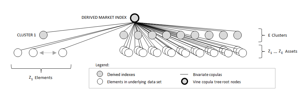
Figure 4: Diagrammatic representation of the first tree in the CDCV model.

A fitting algorithm for the CDCV model is also provided in Appendix A.7, which loops through each cluster, fitting firstly the cluster index to market index unconditional copula and secondly the asset to market index unconditional copulas. This process fits the first C-Vine tree of the CDCV model, as illustrated in Figure 4. In doing so, we transform the cluster index and asset time series using the fitted parameters and appropriate $h$-function for the AIC-selected copula family.

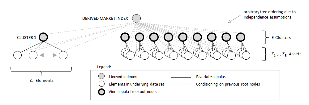
Figure 5: Diagrammatic representation of the subsequent trees in the CDCV model, with cluster indexes as root nodes.

The CDCV model’s fitting algorithm is a simple extension of the C-Vine algorithm, based on the method of [9]. The primary differences between the CDCV and C-Vine fitting algorithms are that the CDCV algorithm fits a multivariate copula after fitting a specified number of trees (i.e., it is a simplified C-Vine), it incorporates the concept of clustering and it incorporates independence assumptions between elements and indexes from other clusters. After fitting the first tree of the CDCV model, we then fit a conditional copula between each asset and its associated cluster index (i.e., conditional upon the market index), as illustrated in Figure 5.

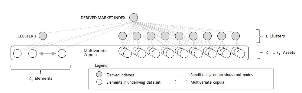
Figure 6: Diagrammatic representation of the CDCV model’s jointly-simplifying multivariate copula.

Finally, we fit a Student’s-t or Gaussian multivariate copula to the conditioned assets, as illustrated in Figure 6. A similar adaption of the C-Vine simulation algorithm (given in Appendix A.6) enables us to easily simulate from the CDCV model, as detailed in Appendix A.8.

3 Analysis, Results and Conclusions

In order to demonstrate that our CDCV model is capable of providing improved results over equivalent fixed-hierarchy models in the literature, we implement first a version of the Heinen & Valdesogo CAVA model selecting between the marginal distributions, bivariate copulas and multivariate copulas described in Section 2.3. We then implement the CDCV model by replacing the externally sourced S&P 500 indexes with the CDCV model’s derived indexes as outlined in Section 2.2, before then also relaxing the fixed clustering structure and allowing it to vary through time based on the clustering methodology detailed in Section 2.1.

3.1 Data

To test both the CDCV and CAVA implementations with clusters of varying size, we select the S&P 500 market and 10 industry sector indexes, plus 62 of the 95 assets that [9] analysed.

H&V Sector	Largest 5 Stocks by Market Cap June 2008					Smallest 5 Stocks by Market Cap June 2008
ENERGY	XOM	CVX	COP	SLB	OXY	RDC	TSO
INDUSTRIAL	GE	UTX	BA	MMM	CAT	PLL	R	CTAS	RHI
HEALTH	JNJ	PFE	MRK	ABT		PKI	THC
FINANCIAL	BAC	JPM	C	AIG	WFC	HBAN
UTILITIES	EXC	SO	D	DUK		TEG	TE	PNW	CMS	GAS
MATERIALS	DD	DOW	AA	PX	NUE	IFF	BMS
CONS DISCR	MCD	CMCSA	DIS	HD
CONS STAP	PG	WMT	KO	PEP	CVS	BF.B
IT	MSFT	IBM	AAPL	CSCO	INTC
TELECOM	T	VZ	CTL

Table 1: Details of the assets we use for analysing the CDCV model. These are 62 of the 95 assets used by Heinen & Valdesogo to test their CAVA model, and provide us with variation in the number of stocks from each industry.

For these stocks and indexes, we obtained from Bloomberg daily return values between 1st January 2005 and 18th December 2008 to analyse performance both prior to and during the recent financial crisis.

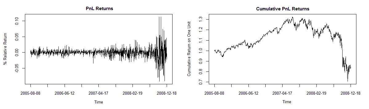
Figure 7: Daily and cumulative relative returns PnL of an equally weighted portfolio of the 62 assets in Table 1, between 8th August 2005 and 18th December 2008 (i.e., excluding the initial 150 days learning period).

This data is illustrated in Figure 7, showing the daily and cumulative relative returns for an evenly weighted portfolio of the 62 marginals, with an average daily return of $0.00002$% and a variance of $0.00052$%. The distribution of these asset return means is illustrated in Figure 8, and clearly shows that the presence of negative skew in the asset returns. We also note that these 62 marginal distributions have a mean kurtosis of $12.48$, and a minimum kurtosis of $3.416$, which strongly indicates that we have non-Gaussian marginals.

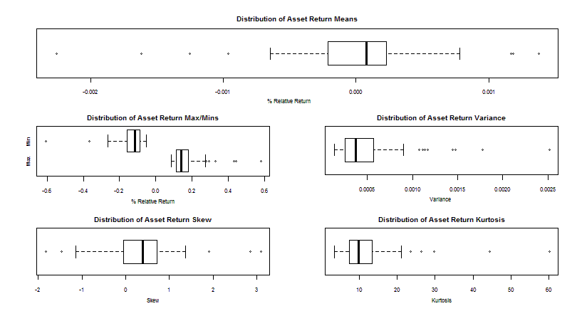
Figure 8: Distribution of the 62 relative asset return means, maxima, minima, variance, skew and kurtosis, where the statistics of each marginal distribution are obtained directly from the data between 8th August 2005 and the 18th December 2008 (i.e., excluding the initial 150 days learning period).

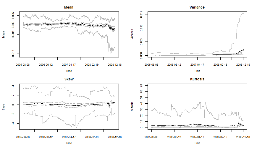
Figure 9: Mean (black) and quantiles (grey) q1, q25, q50, q75, q99 of the 62 marginals’ relative asset return mean, variance, skew and kurtosis statistics through time, based on a 150 day rolling learning period.

In the following analysis, we are also interested in the time-varying performance of the CDCV and CAVA models; an aspect of market sector model performance not directly addressed by either [9] or [5], or the related literature. To support this analysis, we illustrate in Figure 9 the time-dependent variation of the marginal data statistics from Figure 8. Of particular interest to us are the 1st and 99th quantiles of each distributional statistic, as these are likely to be the most severe violations of any marginal assumptions that we may make. Figure 9 also validates our use of the Student’s-t distribution to capture excess kurtosis in the marginals and the Skew-Student’s-t distribution to capture excess skew.

3.2 Model Fitting Performance

To demonstrate that the more generalised structure of the CDCV model is capable of outperforming the CAVA model’s rigid hierarchy, we first replicate here the primary measures of performance analysis that [9] employed, before extending the analysis to consider other aspects of model performance.

		Distribution of Bivariate Rank Correlations
Conditioning	Model		Mean	Std Dev	q1	q25	q50	q75	q99
None	Both		0.3506	0.1258	-0.0246	0.2671	0.3474	0.4291	0.8597
Market	CDCV		0.0022	0.1575	-0.4387	-0.0971	-0.0037	0.0860	0.7638
	CAVA		0.0116	0.1505	-0.4060	-0.0814	0.0009	0.0841	0.7782
Market + Cluster	CDCV		-0.0023	0.0936	-0.4319	-0.0625	-0.0016	0.0588	0.3795
Market + Sector	CAVA		0.0013	0.0950	-0.4835	-0.0606	0.0020	0.0642	0.3657
		Distribution of (Absolute) Bivariate Rank Correlations
Conditioning	Model		Mean	Std Dev	q1	q25	q50	q75	q99
Market + Cluster	CDCV		0.0733	0.0583	0.0001	0.0287	0.0607	0.1040	0.4670
Market + Sector	CAVA		0.0747	0.0587	0.0001	0.0296	0.0625	0.1065	0.4981

Table 2: Distributional statistics of all bivariate asset correlations, at various stages of the conditioning process employed when fitting CAVA and CDCV (clusters$=15$, noise parameter $\Upsilon=11$) models to a rolling learning period of 150 days.

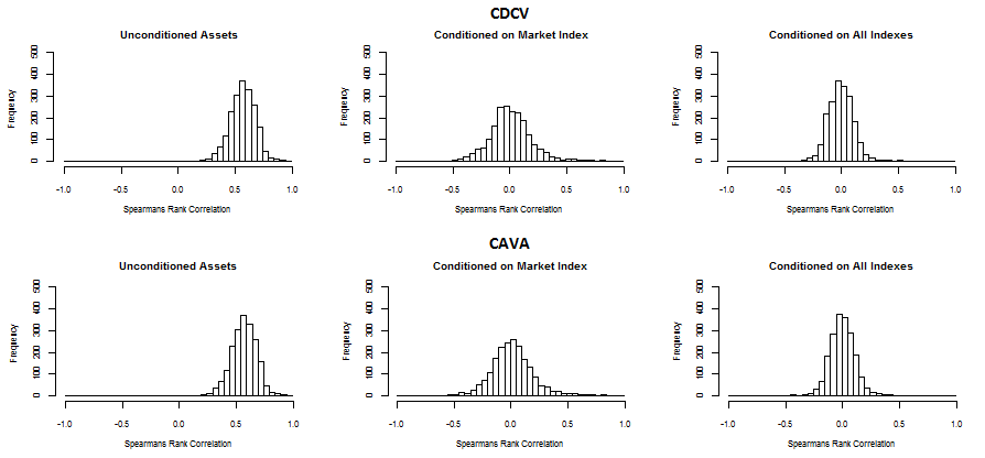
Figure 10: Distributions of all bivariate Spearman’s Rho rank correlations between assets, at various stages of the conditioning process employed when fitting the CAVA and CDCV models to a rolling learning period of 150 days.

In each time step of our data, we fit both the CDCV and CAVA implementations to a rolling learning period of $150$ daily returns. The CDCV model parameters are chosen to include a Kendall’s Tau based distance metric, an Adapted Single Linkage Criterion, a fixed number of clusters set at $15$ and a volatility-weighted mean index construction with a noise parameter of $\Upsilon=1/\lambda=11$. These parameters were chosen based on a cursory performance analysis and will be used throughout this section before we analyse optimal parameter choices in Section 3.8. We then record the distribution of bivariate Spearman’s Rho rank correlations remaining between pairs of asset return time series after conditioning our data on first the market index and then the sector/cluster indexes as illustrated in Figure 10. The resulting distributive statistics are then summarised across all $850$ time steps in Table 2, as an indicator of the model’s ability to capture the dependence in our data set.

These results indicate that while the market index conditioning of the CDCV implementation is out-performed slightly by the CAVA implementation, the fully conditioned results of the CDCV improve upon those of the CAVA implementation despite having only performed a cursory parameter analysis. In particular, the CDCV implementation results in a slightly lower standard deviation of $0.0936$ as opposed to the CAVA’s $0.0950$. When the absolute rank correlations are considered, the mean, standard deviation and all quantile values are lower than the corresponding CAVA results, with the remaining maximum absolute correlation $6.2\%$ lower than the equivalent CAVA value. The CDCV model’s absolute q50 percentile value represents a $2.8\%$ drop in the bivariate correlation remaining, while the absolute q25 percentile value represents a $3.0\%$ drop. The graphical summary of these results, presented in Figure 10, illustrates that the CDCV and CAVA implementations also lead to similar distributions of remaining bivariate correlations. However, in order to assess more fully the performance of the two models we must analyse how these distributions vary through time.

3.3 Stability Analysis

In Figure 11, we show the evolution of the CDCV bivariate rank correlation quantile values from Table 2, illustrating how the range of rank correlations in the data varies through time.

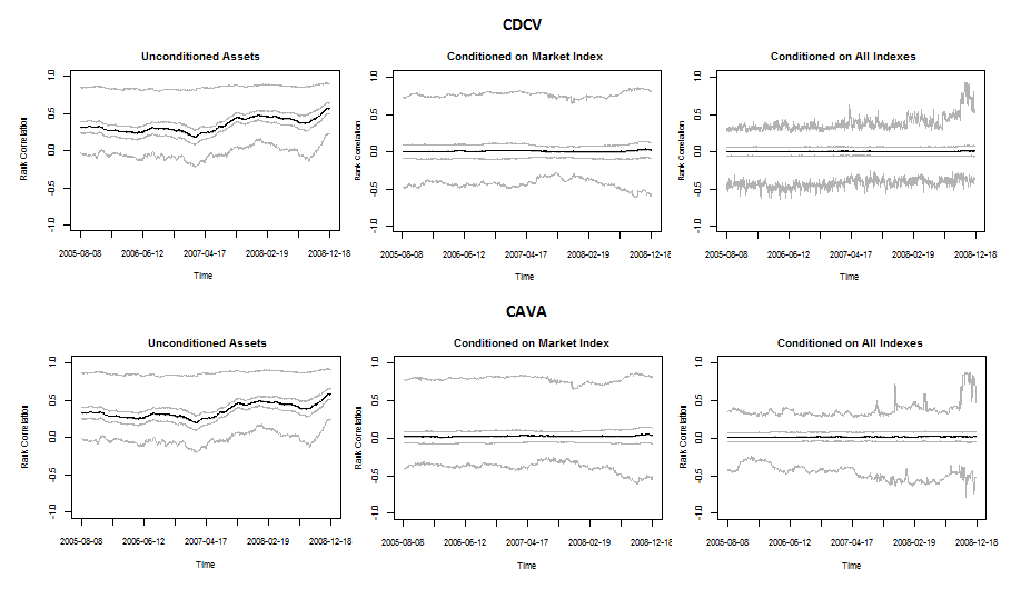
Figure 11: Evolution through time of the distributional statistics (q1, q25, q50, q75, q99) of all bivariate correlations between assets, at various stages of the conditioning process employed when fitting the CAVA and heuristically optimised CDCV models to a rolling learning period of 150 days.

In line with Figure 10, the conditioning on the market index in Figure 11 appears to consistently shift the mean and median of the conditioned distribution towards zero, while introducing a positive skew in the correlation distribution. The subsequent conditioning on the cluster indexes then significantly reduces the skew, while focusing the 25th and 75th quantiles more closely around zero. While the model fitting looks largely stable, some minor variability is introduced in the quantiles due to the flexibility of the CDCV model’s structure, which is allowed to vary in each time step. However, this analysis also indicates that the CDCV model produces more stable values than the CAVA structure, which may be due to the dampening effect of the noise term used when constructing the CDCV model’s derived indexes (see Section 2.2). Figure 11 also illustrates that both our implementations are equally unable to capture the most extreme positive correlations that occur in late 2008. As our analysis is primarily comparative we do not address this point further here, but an area for further research would be to investigate further whether the model could be improved to also capture these most extreme dependencies, for example by selecting from a larger set of bivariate copulas.

	Model	8-8-05	9-1-06	12-6-06	9-11-06	17-4-07	17-9-07	19-2-08	21-7-08	18-12-08	Mean
	CDCV	166	177	166	168	186	190	179	192	215	182
	CAVA	157	172	172	172	181	177	176	185	220	157

Table 3: The number of copula parameters fitted by the heuristically optimised (15 clusters; noise parameter, $\Upsilon=11$) CDCV and the CAVA models through time.

A final component of this analysis is detailed in Table 3, which illustrates the variation in the number of parameters to be fitted through time. The number of parameters utilised by both the CDCV and CAVA implementations increases substantially during times of market stress, primarily due to the increase in the number of Student’s-t copulas selected.

3.4 VaR Backtesting

Another comparison that we provide between the CDCV and CAVA implementations is their Value-at-Risk (VaR) backtesting performance, based on an analysis of the number of VaR breaches that occur during within-sample and out-of-sample testing and the associated Proportion of Failures (PoF) test statistic of unconditional coverage given by [14] as

$$LR_{PoF}=-2\ln\left(\frac{\left(1-q\right)^{T-x}q^{x}}{\left(1-\left(\frac{x}{T}\right)\right)^{T-x}\left(\frac{x}{T}\right)^{x}}\right)\,,$$

where $x$ is the number of exceptions, $T$ is the total number of trials (time steps) and the test statistic is asymptotically distributed as $LR_{PoF}\thicksim\chi_{1df}^{2}$. As our analysis is focused on the performance of high-dimensional portfolios we are content for now to calculate the vector of theoretical VaR quantiles using an equally weighted portfolio of all 62 assets considered in this analysis. We leave a more thorough review of sub-portfolio backtesting performance and conditional coverage as topics for further analysis.

When testing the CDCV model within-sample, we obtain a $VaR_{95}$ p-value of $0.250$ under the null hypothesis $H_{0}$ that the actual exception rate $q$ equals the observed exceptions rate $\hat{q}$ (where an exception is deemed to be a breach of the predicted $95$% VaR threshold), and thus we can comfortably accept $H_{0}$ at any reasonable level of confidence (see Table 4). When considering the more extreme $99^{th}$ percentile loss we obtain a $VaR_{99}$ p-value of $0.043$ and so would narrowly reject $H_{0}$ at the $95\%$ confidence level, while continuing to accept it if we test at the $99\%$ confidence level.

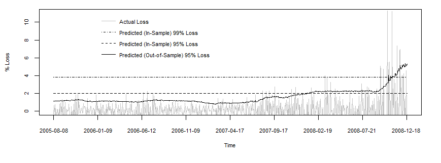
Figure 12: VaR back-testing performance of the CDCV model: Actual % losses plotted against the out-of-sample 95th percentile loss vector plus the within-sample predicted 95th and 99th percentile loss vectors, based on an equally weighted portfolio of all 62 in-scope assets.

	Model	$\alpha$		$VaR_{\alpha}$	Hits	Hit %	$LR_{POF}$	p-Value	95% Conf	99% Conf
	CDCV	95		1.97	50	5.88	1.322	0.250	Accept $H_{0}$	Accept $H_{0}$
	CAVA	95		1.90	52	6.12	2.093	0.147	Accept $H_{0}$	Accept $H_{0}$
	CDCV	99		3.80	15	1.76	4.090	0.043	Reject $H_{0}$	Accept $H_{0}$
	CAVA	99		3.70	16	1.88	5.308	0.021	Reject $H_{0}$	Accept $H_{0}$

Table 4: Within-sample Value at Risk ($VaR_{95}$ & $VaR_{99}$) backtesting results for the CDCV and CAVA implementations. “Hits” are deemed to be breaches of the relevant $VaR_{\alpha}$ threshold.

In the context of this analysis, we may equate the acceptance of $H_{0}$ to a validation of the $VaR_{\alpha}$ number(s) generated by the model, indicating that the model fits the historical data sufficiently, in so far as that can be assessed by considering the $\alpha-level$ percentile loss. Repeating this test for our model using the CAVA industry hierarchy, we also accept $H_{0}$ under the same conditions as for the CDCV model, albeit with the lower $VaR_{95}$ and $VaR_{99}$ p-values of $0.147$ and $0.021$ respectively. This suggests that the CDCV implementation provides a slightly better PoF backtesting performance than the CAVA implementation for this set of test data.

When we extend this analysis to consider out-of-sample testing by fitting a rolling $150$-day window and generating the predicted $VaR_{95}$ value in each time step, we obtain a breach percentage of $8.23$% ($70$ breaches) for both the CDCV and the CAVA models, with a resultant Kupiec test statistic of $LR_{POF}=15.806$ and a p-value of $\leq 0.01$, leading us to clearly reject the null hypothesis. This is reflective of the difficulties of predictive modelling, and the effects of model risk during significant market shifts or downturns, as illustrated in Figure 12. If we consider the first $750$ time steps only (and disregard the final $100$ which represent the beginning of the 2008 financial crisis), we obtain an out-of-sample $VaR_{95}$ breach percentage of $6.8$%, which gives a Kupiec test statistic of $LR_{POF}=4.621$ and results in a p-value of $0.032$. Under these circumstances, we would accept $H_{0}$ at the $99$% confidence level, but continue to reject it (and accept the alternative hypothesis $H_{1}$) at the $95$% confidence level.

3.5 Copula Fitting & Selection Analysis

We next extend our analysis of the CDCV and CAVA model fitting evolution by reviewing the variation through time in the percentage of copulas selected for both the unconditional copulas in the first tree and the conditional copulas in the subsequent trees.

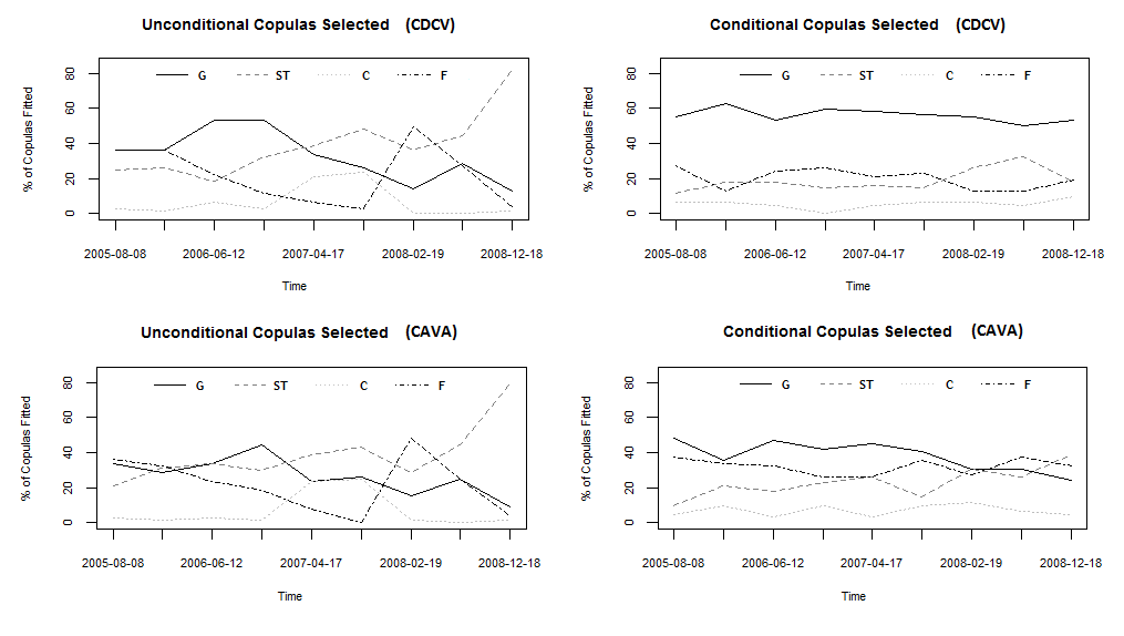
Figure 13: Evolution through time of the number of unconditional and conditional copulas fitted as Gaussian (G), Student’s-t (ST), Clayton (C) or Frank (F) by the CDCV and CAVA models, where we have discretised the data into 9 time steps between 8th August 2005 and the 18th December 2008 in order to minimise noise and clearly illustrate trends.

As shown in Table 5 and Figure 13, the primary difference between the CDCV and CAVA copula fitting evolutions is that after conditioning on the market index, the CDCV model then selects a largely time-consistent proportion of each copula type, with Gaussian copulas being selected $56$% of the time. In comparison, the CAVA implementation selects Gaussian copulas only $39$% of the time (on average), and the actual number selected decreases over $20$ percentage points throughout the backtesting time frame, while the number of Student’s-t copulas increases by over $20$ percentage points. This may be attributable to the direct link between the CDCV model’s derived cluster indexes and the market index, which is a weighted average of the cluster indexes. As this similarity can reasonably assumed to be more pronounced than between the S&P 500 and S&P Industry Sector indexes (due to the inclusion of many other equities in those indexes), we may expect that the first level of conditioning on the CDCV model’s market index would capture a greater proportion of the non-Gaussian cluster index behaviours than in the CAVA framework.

	Model	Root Node		G (%)	ST (%)	C (%)	F (%)
	CDCV	Market Index		35.58	36.51	6.21	21.70
		Cluster Indexes		56.09	19.06	5.47	19.37
	CAVA	Market Index		30.49	39.78	6.81	22.92
		Cluster Indexes		39.02	23.61	8.39	28.98

Table 5: Percentages (averaged across all time steps) of unconditional and conditional copulas fitted as Gaussian (G), Student’s-t (ST), Clayton (C) or Frank (F) by the CDCV and CAVA models in a given time step, based on a 150 day rolling learn period.

Another notable feature of the unconditional copulas selected by both models over the sample period is that the number of Student’s-t copulas fitted increases roughly in response to the increase in market turbulence. At the height of the financial crisis in 2008, the Student’s-t copula accounted for 66 (86%) of the CDCV model’s unconditional copulas between the market index and both asset returns and cluster indexes, as shown in Table 6.

Root Node	Copula	8-8-05	9-1-06	12-6-06	9-11-06	17-4-07	17-9-07	19-2-08	21-7-08	18-12-08	Mean
Market Index	G	27	24	42	47	25	19	12	21	7	21.70
	ST	21	21	14	19	32	38	28	36	66	27.40
	C	2	1	4	1	14	18	0	0	1	4.78
	F	27	31	17	10	6	2	37	20	3	16.71
Cluster Indexes	G	41	33	28	33	34	37	38	33	36	34.78
	ST	5	16	12	9	14	12	11	16	9	11.82
	C	4	2	4	1	3	4	3	4	5	3.39
	F	12	11	18	19	11	9	10	9	12	12.01
Joint-Simplified	G	0	0	0	0	0	0	0	0	0	0
	ST	1	1	1	1	1	1	1	1	1	1

Table 6: Numbers of bivariate copulas fitted to the previous 150 business days (the learning period) for each of the 9 discretised time steps illustrated earlier in Figure 13, broken out into copulas rooted at the market node, copulas rooted at the cluster nodes and multivariate jointly-simplifying copulas.

In our analysis we also see interesting swells in the selection of first Clayton and then Frank copulas in 2007 and then early 2008 respectively, where the increase in the numbers of Clayton copulas coincides with the maximal negative skew and kurtosis values observed in the marginal data, and the increase in the number of Frank copulas selected coincides with the steady decrease in skew and kurtosis illustrated earlier in Figure 9. This behaviour seems reasonable, as we would expect Clayton copulas to be selected when there is increased negative tail dependence between both assets and indexes, and the elliptical Frank copula to be selected when such characteristics are reduced. Table 6 also indicates that, for our data set, the Student’s-t multivariate copula is almost always more appropriate than the Gaussian copula for joint simplification. This is reflected in the AIC scores from which the model fitting selection is derived and is consistent with the analysis of [5] which highlights that the choice of a joint Gaussian simplification (per [9]) is often not appropriate.

3.6 Marginal Fitting & Selection Analysis

While the analysis of the marginal distributions over all time steps in Figure 8 indicates that we will rarely need to fit Gaussian marginal distributions, we must recall that (as indicated by Figure 9) the distributions will vary through time when fitted to a rolling learning period.

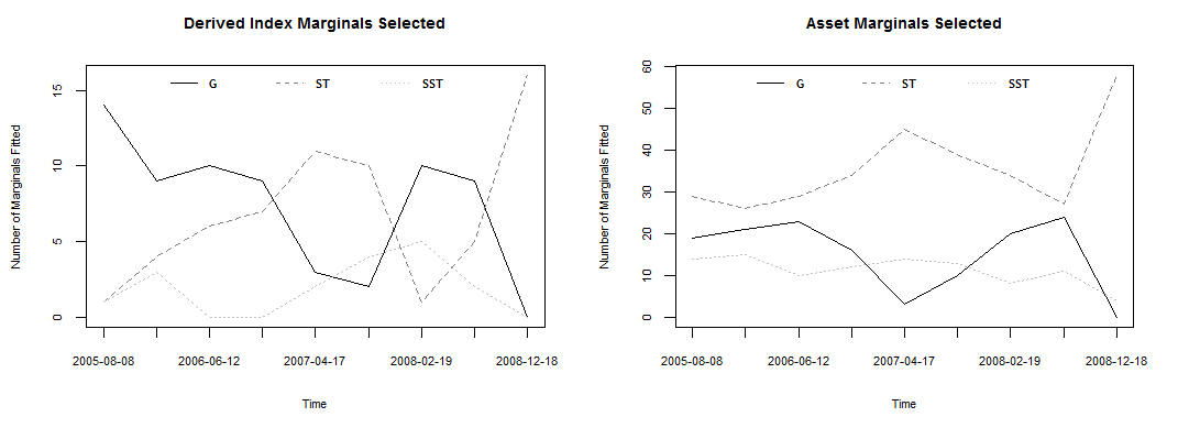
Figure 14: Number of index and asset marginal distributions fitted as Gaussian (G), Student’s-t (ST) and Skew Student’s-t (SST) by the CDCV model, where we have discretised the data into 9 time steps between 8th August 2005 and the 18th December 2008 in order to minimise noise and clearly illustrate trends.

In Figure 14 we have again discretised the data into 9 time steps between 8th August 2005 and the 18th December 2008 in order to minimise noise and clearly illustrate the trends in the number of Gaussian (G), Student’s-t (ST) and Skew-Student’s-t (SST) marginal distributions selected by the CDCV model via AIC. As we might expect, the number of Gaussian marginals selected tends to decrease overall, and does so sharply in 2008 as the financial crisis took hold and non-Gaussian characteristics became more prevalent in the asset returns. The number of Student’s-t marginals selected is shown in Figure 14 to approximately mirror the number of Gaussian marginals selected in that one increases when the other decreases. In the case of the derived cluster indexes (constructed via a volatility-weighted averaging of their constituent cluster assets), we also see similar selection patterns to the asset marginals themselves, but with a relatively increased proportion of Gaussian distributions.

Marginal	Distrib	8-8-05	9-1-06	12-6-06	9-11-06	17-4-07	17-9-07	19-2-08	21-7-08	18-12-08	Mean
Assets (62)	G	19	21	23	16	3	10	20	24	0	15.28
	ST	29	26	29	34	45	39	34	27	58	34.57
	SST	14	15	10	12	14	13	8	11	4	12.57
Indexes (16)	G	11	9	10	9	2	2	12	11	0	8.24
	ST	2	7	6	6	11	9	2	3	16	5.25
	SST	3	0	0	1	3	5	2	2	0	2.31

Table 7: Numbers of each marginal distribution type fitted to the previous 150 business days (the learning period) for each of the 9 discretised time steps illustrated earlier in Figure 14, broken out into marginal distributions of the asset time series and of the derived index time series.

Quantification of these marginal distribution selection results through time is provided in Table 7, which suggests that over all time steps the Student’s-t distribution accounts for more than 50% of all asset marginals selected, while the Gaussian distribution is selected approximately 50% of the time when fitting the derived index marginals. The number of Skew-Student’s-t marginals varies less through time, and is selected for approximately 15% of the asset marginals and 20% of the derived index marginals across all time steps.

3.7 Clustering Analysis

While we have left the optimisation of clustering and index construction methodologies as for further research, we briefly illustrate here the impact of such approaches on the composition of the clusters obtained.

As illustrated in Figure 15, the cluster decomposition obtained when applying the CDCV model to our full analysis time period includes many clusters that are still constructed from within-industry assets, i.e. those from the same industry. However, it can be seen that many of the assets, particularly Health companies, appear in different clusters from their industry peers. We believe that this is a key benefit of the CDCV model’s clustering approach: within any timestep clusters may be formed from assets in different industry groups, but we expect their behaviour to be more closely related during the learning period in question.

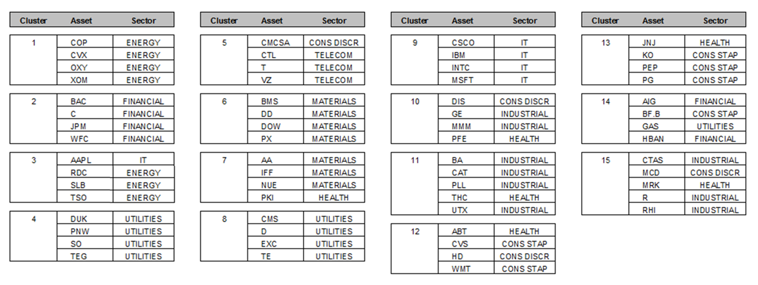
Figure 15: The decomposition of 15 clusters generated using daily returns between 1st January 2005 and 18th December 2008, a Kendall’s Tau based distance metric and an Adapted Single Linkage Criterion.

3.8 Sensitivity Analysis

We next analyse the sensitivity of the CDCV model’s performance to changes in its construction. This is an aspect of these simplified vine copula models that has not been addressed by the existing literature, despite being fundamental to the usability of such models. We do not provide an exhaustive analysis here, but rather provide initial exploratory results that indicate such considerations are material and may indeed have a significant impact on model performance.

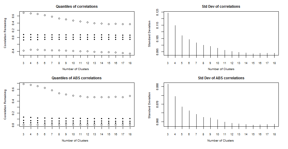
Figure 16: For number of clusters $3\leq N\leq 18$, we plot the quantiles q1, q25, q50, q75, q99 and the standard deviation of the distribution of bivariate rank correlations remaining after conditioning on all nodes of the CDCV model’s vine copula. We also plot equivalent values for the absolute rank correlations remaining. These summary metrics are each derived by averaging the equivalent metrics obtained from model fitting 50 time steps between 1st January 2005 and 18th December 2008, a learning period of 150 days, a vol-weighted index with a noise parameter of $\Upsilon=11$, the Adapted Single Linkage Criterion and a Kendall’s Tau based distance metric.

In Figure 16, we implement the CDCV model with the same parameter settings as in the analysis above, but additionally vary the number of clusters that we construct from the 62 asset time series. For ease of implementation we fit each parameter combination for a sample of 50 time steps and average the results. This figure illustrates that the number of clusters utilised for this data set has a material effect on the standard deviation of the remaining correlations after model fitting the vine, prior to application of the jointly simplifying multivariate copula. In the case where only three clusters were used, this standard deviation rises to 0.12 from its minimum of 0.093 obtained using 15 clusters, suggesting that model performance deteriorates as cluster size increases or as the number of clusters decreases. These results also highlight that when the minimal cluster size decreases (i.e., the number of clusters increases) the high negative correlations that we have attempted to minimise with our index noise parameter(s) are more prevalent. Such findings indicate that the clustering or grouping of a market-sector vine copula model has a material impact on model performance and should be considered by future research in this area.

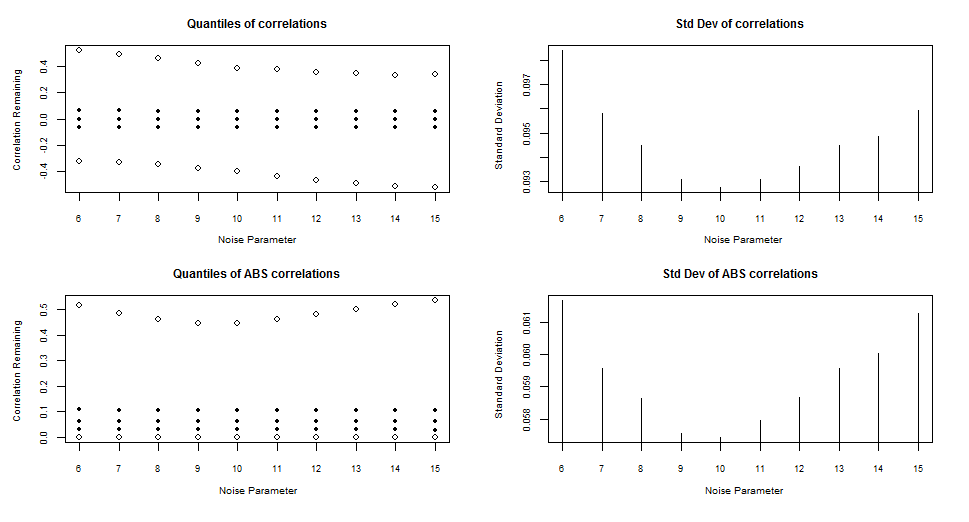
Figure 17: For noise parameter $6\leq\Upsilon\leq 15$, we plot the quantiles q1, q25, q50, q75, q99 and the standard deviation of the distribution of bivariate rank correlations remaining after conditioning on all nodes of the CDCV model’s vine copula. We also plot equivalent values for the absolute rank correlations remaining. Results are obtained from the same setup described in Figure 16, but with an additional requirement for 15 clusters.

In Figure 17, we next vary the scale of the noise term used to construct our indexes. Varying the noise parameter $\Upsilon=1/\lambda$ defined in (8), we observe that as $\Upsilon\rightarrow\infty$ and thus $I_{+}\rightarrow I$ we are left with high negative correlations caused by the similarity between asset and index time series. By introducing increasingly sizable perturbations we suppress the high negative correlations but we also lose some of the ability to condition away the high positive correlations in our clusters. Figure 17 suggests that the optimal noise parameter range for this data set is $9\leq\Upsilon\leq 11$ and illustrates that the detrimental effect of the random noise term on the standard deviation of remaining bivariate rank correlations is minimal for the noise parameter range required to dampen the most extreme negative correlations.

4 Discussion of Findings and Further Areas for Research

The analysis presented in the preceding section suggests that the proposed CDCV model is a viable choice for modelling high dimensional dependence structures in a financial context, and in particular that it is capable of providing increased flexibility and improved performance when compared to the original CAVA model of [9]. That such results are obtainable without the use of externally sourced index time series indicates clearly that future research endeavouring to implement simplified vine copula models need not and should not restrict their analysis to specific hierarchical constructions or data sets. Our analysis demonstrates that the restriction on the clustering structure imposed by the use of market-available external indexes has a material impact on the performance of such vine copula models. In particular, we have shown that the way in which assets are partitioned into clusters, the number of clusters utilised, and the method by which our sector/market indexes are constructed all impact the ability of the model to capture dependence. Whereas [9] tested their CAVA model using ten almost equally-sized industry sectors, and [5] tested their RVMS model using five country-based groupings of varying size, we have tested the CDCV model on a data set from which a variable or fixed number of clusters may be formed in each given time step. We have demonstrated that smaller cluster sizes are preferable for capturing the majority of the bivariate rank correlation, that these small clusters tend to introduce negative dependence into the model and that this may be mitigated in practice by the addition of a small perturbation to the index construction process. While we have only performed a cursory analysis of which clustering rules provide the best model performance, this approach opens up a number areas for further analysis. Critically, we have also shown that the performance of such models is not constant through time. While this may seem an obvious conclusion it is an aspect of these models that has not been fully addressed in the literature to date.

The applications of the CDCV model are significantly more diverse than those of the market-sector models that it extends, due primarily to its abstraction of the modelling framework from the underlying data. While the CDCV model utilises the same hierarchical construction used by [9, 5] and again recently used by the Bi-factor copula model of [11], its primary contribution is the inclusion of a clustering mechanism to render it applicable to all data sets. This is a logical next step to the combination of market-sector and factor-copula models, and continues the theme of abstracting high-dimensional vine copula modelling frameworks from data, as also pursued by [18, 6, 13]. This abstraction makes the CDCV model applicable to the analysis of any set of non-independent variables, although we would expect it to be most appropriate for data sets that are likely to exhibit clustering in a number of dimensions, such as global stock portfolios. In such a financial context, copulas are already used for a variety of purposes; for example to model the dependence between stocks within a basket or to model and simulate expected returns on portfolios of assets. Computationally feasible vine copula models can in turn provide demonstrable improvements over market standard approaches such as multivariate copulas or simple covariance matrices. A purpose for which full vine copula models have already been demonstrated to present such an improvement is the optimisation of high dimensional stock portfolios. For example, [17] showed that a CVaR-optimised portfolio with selection based on a Clayton C-Vine copula model outperforms an equivalent multivariate Clayton copula model for portfolios or 10 or more assets. While fully implemented vine copulas were addressed by the authors, a natural extension of our research would be to assess whether extensions of traditional vine copula models (such as the CDCV model and the models of [18, 6, 11]) provide sufficient accuracy to be practically implemented for such portfolio optimisation.

Appendix A Definitions and Algorithms

A.1 Clustering Rules – Distance Metrics

A selection of distance metrics commonly found in the literature. Note that $\bar{x}_{i,j}$ is the mean $x_{i,j}$ value, A is the set of concordant pairs, B the set of discordant pairs, and $y_{i,j}$ the set of ranked variables derived from the raw $x_{i,j}$ values.

	Distance Metric ($D$)		$=d\left(x_{i},\,x_{j}\right)$, for a pair of vectors $x_{i}$, $x_{j}$ each with $T$ time steps
	Euclidean		$=\sqrt{\sum_{t=1}^{T}\left(\left(x_{i}\right)_{t}-\left(x_{j}\right)_{t}\right)^{2}}$
	Manhattan		$=\sum_{t=1}^{T}\mid\left(x_{i}\right)_{t}-\left(x_{j}\right)_{t}\mid$
	Pearson’s-based		$=\sqrt{2\cdot\left(1-\frac{\sum_{t=1}^{T}\left(\left(x_{i}\right)_{t}-\bar{x}_{i}\right)\left(\left(x_{j}\right)_{t}-\bar{x}_{j}\right)}{\sqrt{\sum_{t=1}^{T}\left(\left(x_{i}\right)_{t}-\bar{x}_{i}\right)^{2}\sum_{t=1}^{T}\left(\left(x_{j}\right)_{t}-\bar{x}_{j}\right)^{2}}}\right)}$
	Kendalls Tau-based		$=\sqrt{2\cdot\left(1-\frac{\sum_{t=1}^{T}1_{A}\left(x_{i},x_{j}\right)_{t}-\sum_{t=1}^{T}1_{B}\left(x_{i},x_{j}\right)_{t}}{\frac{1}{2}n(n-1)}\right)}$
	Spearmans Rho-based		$=\sqrt{2\cdot\left(1-\frac{\sum_{t=1}^{T}\left(\left(y_{i}\right)_{t}-\bar{y}_{i}\right)\left(\left(y_{j}\right)_{t}-\bar{y}_{j}\right)}{\sqrt{\sum_{t=1}^{T}\left(\left(y_{i}\right)_{t}-\bar{y}_{i}\right)^{2}\sum_{t=1}^{T}\left(\left(y_{j}\right)_{t}-\bar{y}_{j}\right)^{2}}}\right)}$

Table A1 : Distance metrics for agglomerative clustering

A.2 Clustering Rules – Linkage Criterion

This table highlights the most common linkage criteria used in the literature, in addition to an Adapted Single criterion that we have introduced. Note that $X_{p},\,X_{q}$ may be either singleton elements or in-progress clusters of size $>1$, where the set of all pairs of non-singleton clusters is denoted by $\Omega$, the maximum cluster size is set by parameter $a$, the maximum number of clusters is set by parameter $b$, and the resultant number of clusters that would exist following a given linkage is denoted by $X^{n}$.

	Linkage Criterion		$=P\left(X_{p},\,X_{q}\right)$, to be linked, given elements $x_{i}$, $x_{j}$ in clusters $X_{p},X_{q}$
	Single		$=\underset{X_{p},X_{q}}{\min}\left\{\underset{i,j}{\min}\left\{d\left(x_{i},\,x_{j}\right)\,:\,x_{i}\in X_{p},\,x_{j}\in X_{q}\right\}\right\}$
	Complete		$=\underset{X_{p},X_{q}}{\min}\left\{\underset{i,j}{\max}\left\{d\left(x_{i},\,x_{j}\right)\,:\,x_{i}\in X_{p},\,x_{j}\in X_{q}\right\}\right\}$
	Average		$=\underset{X_{p},X_{q}}{\min}\left\{\frac{1}{\mid X_{p}\mid\mid X_{q}\mid}\underset{x_{i}\in X_{p}}{\sum}\underset{x_{j}\in X_{q}}{\sum}d\left(x_{i},\,x_{j}\right)\right\}$
	Adapted Single		$=\underset{X_{p},X_{q}}{\min}\left\{\underset{i,j}{\min}\left\{d\left(x_{i},\,x_{j}\right)\,:\,x_{i}\in X_{p},\,x_{j}\in X_{q}\right\}:,\,\left[X_{p},\,X_{q}\right]\notin\Omega,\,X_{p}<a,\,X_{q}<a,\,X^{n}\leq b\right\}$

Table A2 : Linkage criteria for agglomerative clustering

A.3 Clustering Algorithm – Adapted Single

This pseudo code is for a general agglomerative clustering algorithm. Resulting set of clusters is denoted $\Omega$, where R is a pre-defined stopping rule, $l\left(\right)$ is the linkage criterion and $d\left(\right)$ the distance metric. $L_{x,y}$ is the pair of (possibly derived) time series selected from clusters x and y by the linkage criterion, and $D_{x,y}$ is the distance calculated between $L_{x,y}$. Finally, $\|\Omega\|$ is the size of the set of all clusters.

Algorithm to Cluster Assets
Select n asset time series $a_{i};\,i=1,...,n$
$m=n$
Select m clusters $C_{k}=\left\{a_{i};\,a_{i}\in C_{k}\right\};\,k=1,...,m\,;\,i=1,...,n$
$q=0$
Set $R=FALSE$
for $z\leftarrow 1,2,3,...$
$\Omega=\left\{C_{k};\,C_{k}\neq 0\right\}$
Evaluate stopping rule $R$
if $R=TRUE$ or $\|\Omega\|=1$ then
Stop
else if $R=FALSE$ then
for $x\leftarrow 1,2,...,m+q$
for $y\leftarrow 1,2,...,m+q$
if $C_{x}=0$ or $C_{y}=0$
$D_{x,y}=\infty^{+}$
else
$L_{x,y}=l\left(C_{x},\,C_{y};\,\right)$
$D_{x,y}=d\left(L_{x},\,L_{y}\right)$
end if
end for
end for
$J_{x,y}=\left\{\left[x,\,y\right];\,D_{x,y}=\min\left\{D_{x,y}\right\}\right\}$
$C_{m+1+q}=C_{J_{x}}+C_{J_{y}}$
$q=q+1$
$C_{J_{y}}=0$
$C_{J_{x}}=0$
end if
end for
$\Omega=\left\{C_{k};\,C_{k}\neq 0\right\}$

Table A3 : Pseudo-code algorithm for agglomerative clustering of assets

A.4 Index Construction – Example Rules

Index construction methods considered in Section 2.2 for a cluster of $n$ asset timeseries of $T$ timesteps, where $m_{i}$ is the market capitalisation of asset $i$ at a fixed point in time, $\tau_{i}^{t}$ is the sum of Kendall’s Tau values for all within-cluster bivariate pairs that contain asset $i$, d is an arbitrarily defined parameter that increases the severity of a given weighting, and $\sigma_{i}^{t}$ is the volatility of asset $i$. We also define $X$ to be a matrix containing $n$ column vectors $x_{1}^{t},...,x_{n}^{t}$ each of length equal to the learn period used.

	Index		= $I\left(x_{1}^{t},...,x_{n}^{t}\right)$, $\forall t\in\left(1,T\right)$
	Simple Mean		$=\frac{\sum_{i=1}^{n}x_{i}^{t}}{n}$
	“Market Capitalisation” Weighted Mean		$=\frac{\sum_{i=1}^{n}\left(m_{i}x_{i}^{t}\right)}{\sum_{i=1}^{n}m_{i}}$
	“Sum of Kendall’s Tau” Weighted Mean		$=\frac{\sum_{i=1}^{n}\left(\tau_{i}^{t}+d*\left(\tau_{i}^{t}-\min\left\{\tau_{i}^{t}\right\}\right)x_{i}^{t}\right)}{\sum_{i=1}^{n}\left(\tau_{i}^{t}+d*\left(\tau_{i}^{t}-\min\left\{\tau_{i}^{t}\right\}\right)\right)}$
	“Volatility” Weighted Mean		$=\frac{\sum_{i=1}^{n}\left(\sigma_{i}^{t}x_{i}^{t}\right)}{\sum_{i=1}^{n}\sigma_{i}^{t}}$
	1st Principal Component		$=X.\left(\underset{\shortparallel w\shortparallel=1}{\arg\,\max}\left\{\frac{w^{T}X^{T}Xw}{w^{T}w}\right\}\right)$

Table A4 : Construction methods for sector and market indexes

A.5 C-Vine Model-fitting Algorithm

We provide below pseudo-code for a general C-Vine copula fitting algorithm that utilises these $h$-functions, based on the algorithms provided by [1]. In this algorithm we obtain a vector $Q_{ik}\left(\Psi_{ik},\,\Theta_{ik},\,L_{ik}\right)$ of fitted bivariate copulas between the $n$ time series indexed via $i$ and $k$, where each element $Q_{ik}$ consists of a selected copula family $\Psi_{ik}$, and set of fitted parameters $\Theta_{ik}$ and a log-likelihood $L_{ik}$. These values are obtained by application of the functions fitCopula( ) from the package {copula} and AIC( ) from the package {stats}, which perform the bivariate fitting process described in Section 2 for time series already transformed via appropriate probability integral transformations to the $U[0,1]$ space. In this model-fitting algorithm for a C-Vine copula we select between $I$ copula families by AIC during each iteration.

C-Vine Fitting
Introduce $x_{i}$; $i=1,...,n$ time series vectors on $U[0,1]$ to be fitted
for $i\leftarrow 2,3,...,n$
for $k\leftarrow 1,2,...,i\text{\textminus}1$
for $c\leftarrow 1,2,...,I$
$q_{c_{ik}}\left(\psi_{c_{ik}},\,\theta_{c_{ik}},\,l_{c_{ik}}\right)=fitCopula\left(x_{i},\,x_{k};\,\psi_{c_{ik}}=c\right)$
$a_{c_{ik}}=AIC\left(\theta_{c_{ik}},\,l_{c_{ik}}\right)$
end for
$C_{ik}=\left\{c_{ik};\,AIC\left(\theta_{c_{ik}},\,l_{c_{ik}}\right)=\min\left[a_{c_{ik}}\right]\right\}$
$Q_{ik}\left(\Psi_{ik},\,\Theta_{ik},\,L_{ik}\right)=q_{C_{ik}}$
$x_{i}=h_{\Psi_{ik}}\left(x_{i},\,x_{k};\,\Theta_{ik}\right)$
end for
end for

Table A5 : Pseudo-code algorithm for fitting a full C-Vine copula

A.6 C-Vine Simulation Algorithm

To simulate from a C-Vine, we begin with a random sample $w_{i}$ of data for each of our asset return variables, and then iteratively “un-condition” the sample through each tree of the vine, applying “inverse $h$-functions” at each step as necessary to obtain the value of the previous conditioning variable. This is essentially a reverse version of our C-Vine fitting algorithm, and provides us with a single sample from the vine copula, denoted by the vector $x$. The following simulation algorithm for a C-Vine copula is per [1]. As earlier, we have that $v_{i-j}$ denotes all $v_{i}$ but excluding $v_{j}$.

C-Vine Simulation
Sample $w_{i}$; $i=1;...n$ independent uniform on $[0,1]$
$x_{1}=v_{1,1}=w_{1}$
for $i\leftarrow 2,3,...,n$
$v_{i,1}=w_{i}$
for $k\leftarrow i\text{\textminus}1,i\text{\textminus}2,...,1$
$v_{i,1}=h^{\text{\textminus}1}(v_{i,1},v_{k,k},\Theta_{k,i\text{\textminus}k})$
end for
$x_{i}=v_{i,1}$
if $i==n$ then
Stop
end if
for $j\leftarrow 1,2,...,i\text{\textminus}1$
$v_{i,j+1}=h(v_{i,j},v_{j,j},\Theta_{j,i\text{\textminus}j})$
end for
end for

Table A6 : Pseudo-code algorithm for simulating from a full C-Vine copula

A.7 CDCV Model-fitting Algorithm

We provide an algorithm for fitting the CDCV Model in Table A7, where $w_{E}$ is the sample market index, $w_{Ce}$ is the index for the $e^{th}$ cluster, and $w_{z}^{Ce}$ is the $z^{th}$ sample asset for the $e^{th}$ cluster. We denote the copula family fitted as $\psi$, the fitted copula parameters by $\theta$, the log likelihood as $l$ and the corresponding AIC statistic $a$. The vector of selected copula families is denoted $C$ and stored in $Q$ with parameters and log likelihoods. In this notation there are $E$ clusters and $Z^{e}$ assets within each cluster. We choose from $I$ bivariate copula families in each bivariate fitting and from $J$ multivariate copula families in the joint-simplification process.

CDCV Fitting
Introduce $w_{M}$ time series vector on $U[0,1]$ for the market index
Introduce $w_{Ce}$; $e=1,...,E$ time series vectors on $U[0,1]$ for the derived cluster indexes
Introduce $w_{z}^{Ce}$; $z=1,...,Z^{e},\,e=1,...,E$ time series vectors on $U[0,1]$ for the assets
Define $\psi_{c_{\left(\cdot,\cdot\right)}}$ as the fitted bivariate copula family for the copula $c$
Define $\theta_{c_{\left(\cdot,\cdot\right)}}$ as the fitted bivariate copula parameter(s) for the copula $c$
Define $l_{c_{\left(\cdot,\cdot\right)}}$ as the fitted bivariate copula log likelihood for the copula $c$
Define $q_{c_{\left(\cdot,\cdot\right)}}$ as a vector containing fitted copula families, parameters and log likelihoods
Define $a_{c_{\left(\cdot,\cdot\right)}}$ as a vector containing AIC values
Define simplified notation for sector to market pairs: $\Lambda=\left(w_{Ce},w_{M}\right)$
Define simplified notation for asset to market pairs: $\Pi=\left(w_{z}^{Ce},w_{M}\right)$
Define simplified notation for asset to sector pairs: $\Omega=\left(w_{z}^{Ce},w_{Ce}\right)$
Define simplified notation for the set of all assets: $\diamondsuit=\left(w_{1}^{C_{1}},...,w_{Z^{1}}^{C_{1}},......,w_{1}^{C_{E}},...,w_{Z^{E}}^{C_{E}}\right)$
## Loop Through Clusters ##
for $e\leftarrow 1,2,...,E$
## Fit Cluster Index to Market Index Copula ##
for $c\leftarrow 1,2,...,I$
$q_{c_{\Lambda}}\left(\psi_{c_{\Lambda}},\,\theta_{c_{\Lambda}},\,l_{c_{\Lambda}}\right)=fitCopula\left(w_{Ce},\,w_{M};\,\psi_{c_{\Lambda}}=c\right)$
$a_{c_{\Lambda}}=AIC\left(\theta_{c_{\Lambda}},\,l_{c_{\Lambda}}\right)$
end for
$C_{\Lambda}=\left\{c_{\Lambda};\,AIC\left(\theta_{c_{\Lambda}},\,l_{c_{\Lambda}}\right)=\min\left[a_{c_{\Lambda}}\right]\right\}$
$Q_{\Lambda}\left(\Psi_{\Lambda},\,\Theta_{\Lambda},\,L_{\Lambda}\right)=q_{C_{\Lambda}}$
$w_{Ce}=h_{\Psi_{\Lambda}}\left(w_{Ce},\,w_{M};\,\Theta_{\Lambda}\right)$
## Loop Through Assets ##
for $z\leftarrow 1,2,...,Z^{e}$
## Fit Asset to Market Index Copula ##
for $c\leftarrow 1,2,...,I$
$q_{c_{\Pi}}\left(\psi_{c_{\Pi}},\,\theta_{c_{\Pi}},\,l_{c_{\Pi}}\right)=fitCopula\left(w_{z}^{Ce},\,w_{M};\,\psi_{c_{\Pi}}=c\right)$
$a_{c_{\Pi}}=AIC\left(\theta_{c_{\Pi}},\,l_{c_{\Pi}}\right)$
end for
$C_{\Pi}=\left\{c_{\Pi};\,AIC\left(\theta_{c_{\Pi}},\,l_{c_{\Pi}}\right)=\min\left[a_{c_{\Pi}}\right]\right\}$
$Q_{\Pi}\left(\Psi_{\Pi},\,\Theta_{\Pi},\,L_{\Pi}\right)=q_{C_{\Pi}}$
$w_{z}^{Ce}=h_{\Psi_{\Pi}}\left(w_{z}^{Ce},\,w_{M};\,\Theta_{\Pi}\right)$
## Fit Asset to Cluster Index Copula ##
for $c\leftarrow 1,2,...,I$
$q_{c_{\Omega}}\left(\psi_{c_{\Omega}},\,\theta_{c_{\Omega}},\,l_{c_{\Omega}}\right)=fitCopula\left(w_{z}^{Ce},\,w_{Ce};\,\psi_{c_{\Omega}}=c\right)$
$a_{c_{\Omega}}=AIC\left(\theta_{c_{\Omega}},\,l_{c_{\Omega}}\right)$
end for
$C_{\Omega}=\left\{c_{\Omega};\,AIC\left(\theta_{c_{\Omega}},\,l_{c_{\Omega}}\right)=\min\left[a_{c_{\Omega}}\right]\right\}$
$Q_{\Omega}\left(\Psi_{\Omega},\,\Theta_{\Omega},\,L_{\Omega}\right)=q_{C_{\Omega}}$
$w_{z}^{Ce}=h_{\Psi_{\Omega}}\left(w_{z}^{Ce},\,w_{Ce};\,\Theta_{\Omega}\right)$
end for
end for
## Fit Multivariate Copula ##
for $c\leftarrow 1,2,...,J$
$q_{c_{\diamondsuit}}\left(\psi_{c_{\diamondsuit}},\,\theta_{c_{\diamondsuit}},\,l_{c_{\diamondsuit}}\right)=fitCopula\left(w_{1}^{C_{1}},...,w_{Z^{1}}^{C_{1}},......,w_{1}^{C_{E}},...,w_{Z^{E}}^{C_{E}};\,\psi_{c_{\diamondsuit}}=c\right)$
$a_{c_{\diamondsuit}}=AIC\left(\theta_{c_{\diamondsuit}},\,l_{c_{\diamondsuit}}\right)$
end for
$C_{\diamondsuit}=\left\{c_{\diamondsuit};\,AIC\left(\theta_{c_{\diamondsuit}},\,l_{c_{\diamondsuit}}\right)=\min\left[a_{c_{\diamondsuit}}\right]\right\}$
$Q_{\diamondsuit}\left(\Psi_{\diamondsuit},\,\Theta_{\diamondsuit},\,L_{\diamondsuit}\right)=q_{C_{\diamondsuit}}$

Table A7 : Pseudo-code algorithm for fitting a CDCV copula model

A.8 CDCV Simulation Algorithm

For the simulation algorithm we start by simulating the asset return random variables from a multivariate copula rather than from a standard uniform distribution. In this simulation algorithm for a CDCV copula model, $h_{\Psi_{\Omega}}^{-1}\left(\cdot\right)$ utilises the $Q_{\Omega}$ conditional fitting results and thus we need not include an h-function. This is in line with the approach of [9] but differs from the C-Vine algorithm in Table A6 which assumes that families and parameters were obtained by fitting unconditional copulas.

CDCV Simulation
Load multivariate fitting output $Q_{\diamondsuit}\left(\Psi_{\diamondsuit},\,\Theta_{\diamondsuit},\,L_{\diamondsuit}\right)$
Load bivariate fitting output $Q_{i}\left(\Psi_{i},\,\Theta_{i},\,L_{i}\right)$ for $i=\left\{\Lambda,\Pi,\Omega\right\}$
Sample $w_{i}$; $i=1;...n$ from multivariate copula family $\Psi_{\diamondsuit}$ with parameters $\Theta_{\diamondsuit}$
## Loop Through Clusters ##
for $e\leftarrow 1,2,...,E$
## Loop Through Assets ##
for $z\leftarrow 1,2,...,Z^{e}$
## ‘‘Un-condition’’ on the Cluster Index ##
$w_{z}^{Ce}=h_{\Psi_{\Omega}}^{-1}\left(w_{z}^{Ce},\,w_{Ce};\,\Theta_{\Omega}\right)$
## ‘‘Un-condition’’ on the Market Index ##
$w_{z}^{Ce}=h_{\Psi_{\Pi}}^{-1}\left(w_{z}^{Ce},\,w_{Ce};\,\Theta_{\Pi}\right)$
end for
end for

Table A8 : Pseudo-code algorithm for simulating from a CDCV copula model

References

- [1] K. Aas, C. Czado, A. Frigessi, and H. Bakken. Pair-copula constructions of multiple dependence. Insurance, Mathematics and Economics, 44(2):182–198, 2009.
- [2] H. Akaike. A new look at the statistical model identification. IEEE Transactions on Automatic Control, 19(6):716–723, December 1974.
- [3] T. Bedford and R. M. Cooke. Vines–a new graphical model for dependent random variables. The Annals of Statistics, 30(4):1031–1068, August 2002.
- [4] E. C. Brechmann. Hierarchical Kendall copulas: Properties and inference. Canadian Journal of Statistics, 42(1):78–108, 2014.
- [5] E. C. Brechmann and C. Czado. Risk management with high-dimensional vine copulas: An analysis of the Euro Stoxx 50. Statistics & Risk Modeling, 30(4):307–342, 2013.
- [6] E. C. Brechmann and H. Joe. Parsimonious parameterization of correlation matrices using truncated vines and factor analysis. Computational Statistics & Data Analysis, 77(0):233–251, 2014.
- [7] U. Cherubini, E. Luciano, and W. Vecchiato. Copula Methods in Finance. The Wiley Finance Series. Wiley, 2004.
- [8] B. S. Everitt, S. Landau, and M. Leese. Cluster Analysis. A Hodder Arnold Publication. Taylor and Francis, 4th edition, 2001.
- [9] A. Heinen and A. Valdesogo. Asymmetric CAPM Dependence for Large Dimensions: The Canonical Vine Autoregressive Copula Model. SSRN Electronic Journal, 2008.
- [10] H. Joe. Families of m-variate distributions with given margins and […] bivariate dependence parameters. IMS Lecture Notes - Monograph Series, 28(c), 1996.
- [11] H. Joe. Dependence Modeling with Copulas. Chapman & Hall/CRC, 2014.
- [12] H. Joe and J. J. Xu. The Estimation Method of Inference Functions for Margins for Multivariate Models. Technical Report no. 166, Department of Statistics, University of British Columbia, pages 1–21, 1996.
- [13] P. Krupskii and H. Joe. Factor Copula Models for Multivariate Data. J. Multivar. Anal., 120:85–101, September 2013.
- [14] P. Kupiec. Techniques for Verifying the Accuracy of Risk Measurement Models. Journal of Derivatives, 3:73–84, 1995.
- [15] D. Kurowicka and H. Joe. Optimal Truncation of Vines. In Dependence Modeling: Vine Copula Handbook, pages pp. 233–247. Singapore: World Scientific Publishing, 2011.
- [16] D. X. Li. On Default Correlation : A Copula Function Approach. Available at SSRN 187289, 1999.
- [17] R. K. Y. Low, J. Alcock, R. Faff, and T. Brailsford. Canonical vine copulas in the context of modern portfolio management: Are they worth it? Journal of Banking & Finance, March 2013.
- [18] A. K. Nikoloulopoulos and H. Joe. Factor Copula Models for Item Response Data. Psychometrika, pages 1–25, 2013.
- [19] F. Salmon. Recipe for Disaster: The Formula That Killed Wall Street. Wired Magazine, 2009.
- [20] R. Shahid, S. Bertazzon, M. L. Knudtson, and W. Ghali. Comparison of distance measures in spatial analytical modeling for health service planning. BMC health services research, 9:200, January 2009.
- [21] A. Sklar. Fonctions de repartition á n dimensions et leurs marges. Publ. Inst. Statistique Univ. Paris 8, pages 229–231, 1959.