Census of H ii regions in NGC 6754 derived with MUSE: Constraints on the metal mixing scale.

We present a study of the H ii regions in the galaxy NGC 6754 from a two pointing mosaic comprising 197,637 individual spectra, using Integral Field Spectrocopy (IFS) recently acquired with the MUSE instrument during its Science Verification program. The data cover the entire galaxy out to $\sim$2 effective radii ($r_{e}$), sampling its morphological structures with unprecedented spatial resolution for a wide-field IFU. A complete census of the H ii regions limited by the atmospheric seeing conditions was derived, comprising 396 individual ionized sources. This is one of the largest and most complete catalogue of H ii regions with spectroscopic information in a single galaxy. We use this catalogue to derive the radial abundance gradient in this SBb galaxy, finding a negative gradient with a slope consistent with the characteristic value for disk galaxies recently reported. The large number of H ii regions allow us to estimate the typical mixing scale-length ($r_{mix}\sim$0.4 $r_{e}$), which sets strong constraints on the proposed mechanisms for metal mixing in disk galaxies , like radial movements associated with bars and spiral arms, when comparing with simulations. We found evidence for an azimuthal variation of the oxygen abundance, that may be related with the radial migration. These results illustrate the unique capabilities of MUSE for the study of the enrichment mechanisms in Local Universe galaxies.

1 Introduction

Nebular emission lines have been historically the main tool at our disposal for direct measurement of the gas-phase abundance at discrete spatial positions in low-redshift galaxies (e.g. Alloin et al., 1979). They trace the young, massive star component in galaxies, illuminating and ionizing cubic kiloparsec-sized volumes of interstellar medium. Metals play a fundamental role in cooling mechanisms in the intergalactic and interstellar medium, and in processes of star-formation, stellar physics, and planet formation.

Previous spectroscopic studies have unveiled some aspects of the complex processes at play between the chemical abundances of galaxies and their physical properties. These studies have been successful in determining important relationships, scaling laws and systematic patterns (e.g. Lequeux et al., 1979; Diaz, 1989; Zaritsky et al., 1994; Garnett, 2002; Tremonti et al., 2004; Moustakas & Kennicutt, 2006). However, these results are limited by statistics, either in the number of observed H ii regions or in the coverage of these regions across the galaxy surface.

The advent of multi-object spectrometers and IFS instruments with large fields of view (FoV) now offers the opportunity to undertake a new generation of emission-line surveys, based on samples of hundreds of H ii regions and full two-dimensional (2D) coverage of the disks of nearby spiral galaxies (e.g. Rosales-Ortega et al., 2010). One of the most interesting results recently derived using IFS data is that the oxygen abundance gradient seems to present a common slope $\sim$$-$0.1 dex/$r_{e}$ for non-interacting galaxies (Sánchez et al., 2012b, 2014b).

This result agrees with models based on the standard inside-out scenario of disk formation, which predict a relatively quick self enrichment with oxygen and an almost universal negative metallicity gradient once it is normalized to the galaxy optical size (Boissier & Prantzos, 1999, 2000). From the seminal works of Lacey & Fall (1985a), Guesten & Mezger (1982) and Clayton (1987), most numerical models of chemical evolution explain the existence of the radial gradient of abundances by the combined effects of a star-formation rate and an infall of gas, both varying with galactocentric radius (e.g., Mollá & Roy, 1999).

Although there is a large number of studies focused on the analysis of the abundance gradient in galaxies, in contrast, little is known about the possible presence of azimuthal asymmetries in this distribution. Deviations from the radial abundance gradient are well known features in the Milky Way, based on the study of Cepheids and open clusters (e.g., Chiappini et al., 2001; Lépine et al., 2011). However, the situation in other spiral galaxies is less clear, and suffers from poor statistics, either for the low number of H ii regions sampled per galaxy or for the large errors of the abundance estimation. Recently, using wide-field IFS Rosales-Ortega et al. (2011) showed that the radial metallicity gradient of NGC 628 varies slighly for different quadrants, although the differences are comparable to the uncertainties introduced by the adopted estimators of the oxygen abundances. More recently, Li et al. (2013) found marginal evidence for the existence of moderate deviations from chemical abundance homogeneity in the intestellar medium of M101, using a combination of strong-line abundance indicators and direct estimations based on the detection of the [O iii]$\lambda$4363 auroral line.

Despite the advances of recent IFS-surveys in our understanding of the evolution of the chemical enrichment processes in galaxies, they present some limitations. The most important one is the lack of the spatial resolution required to propertly resolve individual small-scale morphological structures, in particular individual H ii regions. The IFS surveys with the best physical resolution, such as PINGS (Rosales-Ortega et al., 2010) or CALIFA (Sánchez et al., 2012a), have $\sim$5 times worst spatial resolution than the typical ground-based imaging surveys. This results in a bias in the detection of H ii regions, that are aggregated based on their spatial vicinity (decreasing their number by a factor three or more), and their spectra are polluted by diffuse gas emission (Mast et al., 2014).

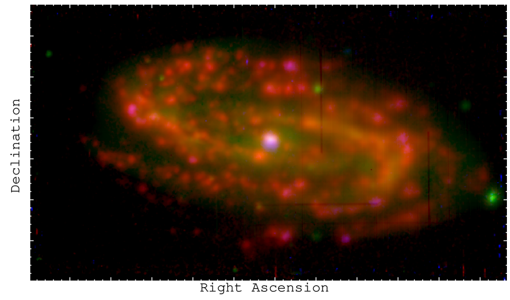
Figure 1: RGB color image of NGC 6754 created using the line intensity maps of [O iii]$\lambda$5007 (blue), $V$-band (green) and H$\alpha$ (red) extracted from the datacubes. Each large tickmark corresponds to 10$\arcsec$ (or 400 pc at the redshift of the galaxy). The green point-like sources are field stars. Each red structure corresponds to a single H ii region.

In principle, the abundance scatter and azimuthal asymmetries of H ii regions around the average radial gradient can be used to constrain the spatial-scale of radial mixing (e.g. Scalo & Elmegreen, 2004; Di Matteo et al., 2013). In the absence of radial mixing the only observed scatter around the abundance gradient should be produced by the errors in the individual measurements. Regardless of its origin (e.g., Athanassoula, 1992), any radial mixing increases the scatter by moving regions of a certain abundance from a certain galactocentric distance to a different one. Therefore, the dispersion around the average slope is a constraint to the maximum radial mixing scale.

So far, for the reasons outlined above, the current IFS surveys lacked the required resolution to address this important key issue in the chemical evolution of galaxies. The Multi Unit Spectroscopic Explorer (MUSE Bacon et al., 2010) has changed dramatically the perspective for these studies. This instrument is a unique tool for the spectroscopic analysis of resolved structures in galaxies, particularly in the local universe. The combination of a large field-of-view (FoV) ($\sim$60$\arcsec$$\times$60$\arcsec$), unprecedented spatial sampling (0.2$\arcsec$/spaxel) for a wide-field IFU, which limits the spatial resolution to the atmospheric seeing, the spectral resolution and large wavelength coverage, and the large aperture of the VLT telescope, makes MUSE a well suited instrument to address these problems. Of course, there are other IFUs with similar or even larger FoVs, like PPAK (Kelz et al., 2006), VIMOS (Le Fèvre et al., 2003) or VIRUS-P (Hill et al., 2008), and also other IFUs operating in the optical range have similar or better spatial sampling, like GMOS (Allington-Smith et al., 2002) or OASIS. However, MUSE is the first one that combines at the same time the large FoV and the image-like spatial sampling.

In this work we study the oxygen abundance gradient of the spiral galaxy NGC 6754 using the data recently observed by MUSE as part of the Science Verification programs (SV). NGC 6754 is a barred Sb galaxy mildly inclined ($i\sim$60^∘). Its brightness (B$\sim$13 mag), projected size (r${}_{25}\sim$ 1$\arcmin$) and redshift ($z=$0.0108), similar to the footprint of the CALIFA galaxies (e.g. Walcher et al., 2014), makes it suitable to perform a census of the H ii regions using MUSE, to further understand the abundance distribution in this galaxy.

2 Data acquisition and reduction

NGC 6754 was observed on June 28th and 30th 2014 in the context of Program 60.A-9329 (PI: Galbany) of the MUSE SV run. The observations were divided into two pointings covering the east and west parts of the galaxy, respectively. The final cube for each pointing is the result of 3 exposures of 900 seconds, where the second and third exposure were slightly shifted (2 arcsec NE and SW, respectively) and rotated 90^∘ from the first exposure, in order to provide a uniform coverage of the field and to limit systematic errors in the reduction.

The reduction of the raw data was performed with Reflex (Freudling et al., 2013) using version 0.18.2 of the MUSE pipeline (Weilbacher et al., 2014), including the standard procedures of bias subtraction, flat fielding, wavelength calibration, flux calibration, and the final cube reconstruction by the spatial arrangement of the individual slits of the image slicers.

The final dataset comprises two cubes of $\sim$100k individual spectra, each covering a FoV slightly larger than $\sim$1^□. Each spectrum covers the wavelength range 4800-9300 Å, with a typical spectral resolution between 1800 and 3600 (from blue to red). The cubes are aligned east-west, with an overlapping area of $\sim$16$\arcsec$, where the galaxy center has been sampled twice. The final mosaiced datacube comprises almost 200k individual spectra, covering the entire galaxy up to 2 effective radii, with a FoV of $\sim$2$\arcmin$$\times$1$\arcmin$. For practical reasons, we analysed each cube separately and later combined the different data products.

Figure 1 illustrates the power of the combined large FoV and high spatial resolution of MUSE, and the quality of the data. It shows a true color image created using a combination of a $V$-band image, and two continuum subtracted narrow-band images of 30Å width, centred in [O iii]$\lambda$5007 and H$\alpha$, at the redshift of the galaxy. The three maps were synthetized from each datacube, and combined to create a single image for each band. For each of the narrow-band images the continuum was estimated from the average of two additional narrow-band images of similar width (i.e., 30Å) extracted at a wavelength redshifted and blueshifted 100Å from the nominal wavelength of the considered emission line at the redshift of the object. Finally, the $V$-band image was synthetized by convolving the spectra at each spaxel by the nominal response curve of the Johnson $V$-band filter. Those images were used to illustrate the spatial resolution and image quality of the data. We should note here than the $V$-band image does not include only continuum emission, since it is contaminated by both H$\beta$ and [O iii]$\lambda$5007, and the H$\alpha$ intensity map is contaminated by the adjacent [N ii] doublet. However, they clearly trace the continuum and emission line distribution across the galaxy. The spatial distribution of the individual H ii /ionized regions can be easily recognized, tracing the star forming regions along the spiral arms of the galaxy. Different seeing conditions for the for the East ($\sim$0.8$\arcsec$) and for the West ($\sim$1.8$\arcsec$) pointings are also clear.

3 Analysis

The main goals of this study are to characterize the abundance gradient in NGC 6754 and to estimate the dispersion of the abundances of the individual H ii regions around the average gradient. In this section we describe briefly how we select the H ii regions, extract and analyze their individual spectra, derive the corresponding oxygen abundance, and analyze their radial gradient. More details on the procedure are described in Sánchez et al. (2012b), and references therein.

3.1 Detection of the ionized regions

The segregation of H ii regions and the extraction of the corresponding spectra is performed using a semi-automatic procedure named HIIexplorer. The details of this program are given in Sánchez et al. (2012b), and a detailed description of the overall detection process, Sánchez et al. (2014b). HIIexplorer requires as input a map of emission line intensities or equivalent widths, a minimum threshold above which the peak intensity of the H ii region is detected, and three different convergence criteria: (i) the maximum fractional difference between the peak intensity and the adjacent ones to be agregated to a particular region, (ii) the minimum absolute intensity for a pixel to be agregated, and (iii) the maximum distance between the pixel considered and the peak intensity . In this particular case we use the map of the equivalent width of H$\alpha$, EW(${H\alpha}$), derived from the narrow-band image described above. The use of the EW guarantees that the analysis is more homogeneous between the two pointings, since this parameter is less affected by possible spectrophotometric differences and it is less sensitive to seeing variations. The fact that the equivalent width may be contaminated or not by the adjacent [N ii] doublet is not relevant, since this map is used only to detect the emission line regions, and not in any further analysis along the article. Therefore, a possible contamination by [NII] may affect only the contrast, and only marginally, but not the detectability of the regions, since the average contamination by this line is about a 30% of the total flux. The output of HIIexplorer is a segmentation map and the integrated spectrum for each of the H ii regions detected.

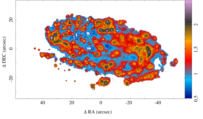
Figure 2: Color coded map of the equivalent width of H$\alpha$ in logarithmic scale. The areas with H$\alpha$ density flux below 1.5 10^-18 erg s^-1 cm^-2 spaxel^-1($\sim$3$\sigma$ detection limit) have been masked. The circles represent the detected H ii regions, width the radius proportional to the extraction aperture.

We processed individually the two datacubes, fixing the input parameters to the optimal ones for the west-pointing, that was observed under worst seeing conditions. We selected a threshold in the peak EW($H\alpha$) = 20Å, and minimum EW($H\alpha$) = 8Å, a minimum fractional peak of 1%, and a maximum distance of 2″. Therefore, the convergence criteria restrict the detection of regions with at least EW($H\alpha$) = 8Å in every spaxel and a maximum diameter of 4″. The selection of these parameters is based on our previous studies with other IFU data and different tests to optimize the results: (i) the minimum absolute EW($H\alpha$) is selected to guarantee that all the pixels agregated to a particular region are above the boundary between retired and star-forming regions proposed by Cid Fernandes et al. (2010) and discussed in Sánchez et al. (2014b), even if a very conservative error of 25% is assumed for this parameter, and/or taking into account the contamination by [N ii]; (ii) the threshold in the peak EW($H\alpha$) is selected to be more than twice the minimum, to guarantee that the region is actually clumpy/peaky, and not a diffuse ionized region; (iii) the maximum distance is fixed to the estimated size of an H ii region, that could have a diameter as large as $\sim$1 kpc (e.g., NGC 5471, Oey et al., 2003; García-Benito et al., 2011), thus, $\sim$4″at the redshift of the object. Using these parameters we detect a similar number of H ii regions in each pointing: 207 in the east pointing and 220 in the west one.

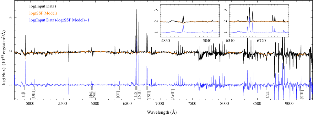
Figure 3: Detail of the spectrum of a typical H ii region extracted from the galaxy. The black line shows the input spectrum in logarithmic scale, together with the best fitted stellar model, in orange. The difference between the logarithms of the input spectrum and the model, shifted by 1, is shown as a blue line. The intensities of the emission lines are so high that the spectra are plotted in logarithmic scale to show them together with the detail of the underlying stellar population. The most prominent spectral features discussed along the article are marked. The spectral regions masked during the fitting of the underlying stellar population are not shown in the orange-solid line. The two boxes show an expanded view around H$\beta$ and H$\alpha$ respectively.

The final catalogue was cleaned for double detections in the overlapping area by removing those H ii regions with coordinates that differ less than 3$\arcsec$. A total of 396 individual clumpy ionized regions are detected, a factor of 5-10 times larger than the number found with lower spatial resolution IFU data (e.g. Sánchez et al., 2013), as predicted by the simulations presented by Mast et al. (2014). Figure 2 shows the EW(${H\alpha}$) map illustrating the result of this procedure. The location and relative size of the H ii regions detected are indicated with black circles. We note here that the HIIexplorer provides with a segmentation map, not with circular apertures. The current representation is therefore illustrative of the size of the H ii regions, but does not show the actual detailed shape of the associated segmented regions for which the spectra are extracted.

3.2 Measurement of the emission line intensities

In this analysis we follow the procedures described in Sánchez et al. (2014b), using the fitting package FIT3D,(Sánchez et al. (2006b, 2011)). We perform a Monte-Carlo fitting using two different single stellar population (SSP) libraries. In order to compare with previous results and provide with useful information of the underlying stellar population, we first use a library that comprises 156 templates to model and remove the underlying stellar population. This library comprises 39 stellar ages, from 1 Myr to 13 Gyr, and 4 metallicities ($Z/Z_{\odot}=$ 0.2, 0.4, 1, and 1.5), and it is described in detail in Cid Fernandes et al. (2013). These templates were extracted from a combination of the synthetic stellar spectra from the GRANADA library Martins et al. (2005) and the SSP library provided by the MILES project (Sánchez-Blázquez et al., 2006; Vazdekis et al., 2010; Falcón-Barroso et al., 2011). Therefore they are restricted to a wavelength range lower than 7000Å. Hence, they cannot be used to remove the underlying stellar population in the full spectral range covered by MUSE. For doing so, we used a more restricted library extracted from the MIUSCAT models (Vazdekis et al., 2012). It comprises 8 stellar ages, from 65 Myr to 17.7 Gyr, and 3 metallicities ($Z/Z_{\odot}=$ 0.4, 1, and 1.5). Our previous experience indicates that to decouple the underlying stellar population from the emission lines a restricted library like this one is enough (e.g. Sánchez et al., 2014a). We do not find large differences between the residual spectra for the wavelength range in common, and therefore we finally adopted the results from the second library for the analysis of the emission lines.

Dust attenuation and stellar kinematics were taken into account as part of the fitting process. The stellar kinematics was derived as a first step, fitting the underlying stellar population with a sub-set of the full stellar library changing the systemic velocity and the velocity dispersion at random within the range of allowed values. Then a first model for the stellar population is derived. This model is used to obtain the dust attenuation, allowed to change randomly within a pre-defined range. The extinction law by Cardelli et al. (1989) was assumed, with a specific dust attenuation of $R_{\rm V}=3.1$. For each iteration over the dust attenuation values a new model of the underlying stellar population is derived. The best combination of the stellar velocity, velocity dispersion and dust attenuation is recovered based on the lowest reduced $\chi^{2}$ provided. Finally, these parameters are fixed and the full stellar library is used to recover the underlying stellar population. Due to the Monte-Carlo fitting adopted, the inaccuracies in the derivation of the underlying stellar population are propagated to the error budget in the emission line fitting, and therefore, into the errors estimated for the emission line fluxes.

Individual emission line fluxes were measured in the stellar-population subtracted spectra by fitting each of them with a single Gaussian function. For this particular dataset we extracted the flux intensity of the following emission lines: H$\alpha$, H$\beta$, [O iii] $\lambda$4959, [O iii] $\lambda$5007, [N ii] $\lambda$6548, [N ii] $\lambda$6583, [S ii] $\lambda$6717, [S ii] $\lambda$6731, [Ar iii] $\lambda$7135 and [S iii] $\lambda$9069. We may notice here that many other relevant emission lines are detected within the wavelength range covered by the spectra. Figure 3 shows a detail of the spectrum of a typical H ii region within the sample, together with the best fitted stellar population model and the resulting emission-line spectrum. In addition to the emission lines measured, it is possible to identify weaker lines like He I $\lambda$5876 and [O I] $\lambda$6300. The two components of the Na I absorption doublet at $\sim$5892Å are clearly resolved, with a contribution due to attenuation that cannot be reproduced by the stellar model, which was actully masked during the fitting process. The prominent CaT$\lambda$8542Å stellar absorptions in the near-infrared is also clearly detected. In addition to the emission line fluxes, we derive the emission line equivalent widths. For doing so, we divide the integrated flux of the line by the median flux density of the best fitted SSP-model in a window of 100Å centred in the wavelength of the emission line. Therefore, these equivalent widths are not contaminated by the contribution of any adjacent emission lines.

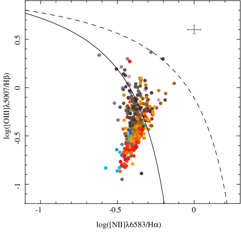
Figure 4: [O iii] $\lambda$5007/H$\beta$ vs. [N ii] $\lambda$6583/H$\alpha$ diagnostic diagram for the 396 H ii ionized regions detected in NGC 6754, color coded by the deprojected galactocentric distance (where bluer colors correspond to the central regions, and reddish-to-grey colors correspond to the outer regions). Solid and dashed lines represent, respectively, the Kauffmann et al. (2003) and Kewley et al. (2001) demarcation curves. They are usually invoked to distinguish between classical star-forming objects (below the solid line), and AGN powered sources (above the dashed line). Regions between both lines are considered intermediate ones. The average error of the line ratios is represented by the error bar in the upper-right corner.

Two artifacts in the spectra are identified in Fig. 3, in particular in the residual emission line spectrum). They look like two bumps at $\sim$4750Å and $\sim$6550Å, just bluewards of H$\beta$ and H$\alpha$. Although they have been masked during the fitting process we prefer to show them in the plot, since they seem to be present in all the MUSE spectra we have analyzed. We are not sure if they are a product of the reduction process or a feature in the raw data. In any case, they do not affect the measurements of the emission lines. Two additional spectral features that are not well reproduced by the SSP models correspond to the Na i$\lambda$5890,5896 absorption feature, at $\sim$5950Å at the redshift of the object, and the CaT$\lambda$8542Å, at $\sim$8630Å at the redshift of the object. The Na i mismatch is a well known feature since this absorption line has two physical origins: (i) the absorption due to the presence of this element in the atmosphere of the stars, which is included in the SSP-templates, and (ii) the absorption due to the presence of this element in the inter-stellar medium, which produces an absorption proportional to the gas content (and dust attenuation). The CaT$\lambda$8542Å is often problematic in the current SSP-templates, that could be related to variations in the IMF, the abundance of Ca, or a non correct understanding of this absorption feature (although it is not the case in the particular example shown in Fig.3, for which we show the prediction from the fitted SSP-model). Due to these well known mismatches, both spectral regions were masked during the fitting process. Residuals from non perfect sky-subtraction of the strong OH-lines in the near-infrared are visible in the redder wavelength ranges, and a clear defect associated with a telluric absoption is shown at $\lambda$$\sim$7600Å. None of the emission lines considered in this study are affected by this later effect.

3.3 Selection of H ii regions

Classical H ii regions are gas clouds ionized by short-lived hot OB stars, associated with ongoing star-formation. They are frequently selected on the basis of demarcation lines defined in the so-called diagnostic diagrams (e.g., Baldwin et al., 1981; Veilleux & Osterbrock, 1987), which compare different line ratios. Figure 4 shows the classical diagram using [O iii]/H$\beta$ vs. [N ii]/H$\alpha$ (Baldwin et al., 1981, BPT diagram hereafter), for the sample of H ii regions described above. This diagnostic diagram is frequently used since it uses very strong emission lines (e.g., Fig.3), and it is less affected by dust attenuation and imperfections in the spectrophotometric calibration. The classical demarcation lines described by Kauffmann et al. (2003) and Kewley et al. (2001) have been included.

In this study we follow Sánchez et al. (2013) to select H ii regions as clumpy ionized regions with EW(H$\alpha$)$>$6Å and located below the Kewley et al. (2001) demarcation curve. This selection guarantees the exclusion of ionized regions possibly dominated by shocks (that are not clumpy in general), regions whose ionization is dominated by post-AGB stars, and AGN-dominated regions (e.g. Cid Fernandes et al., 2010). Following these criteria all the ionized regions selected by HIIexplorer have been classified as H ii regions.

The distribution of H ii regions across the BPT diagram follows the characteristic pattern in Sa/Sb early-type spirals Sánchez et al. (2014a). They are mostly located at the bottom-right end of the classical location of H ii regions in this diagram, with a tail towards the so-called intermediate region between the two demarcation lines described above. Kennicutt et al. (1989) first recognized that H ii regions in the center of galaxies are spectroscopically different from those in the disk in their stronger low-ionization forbidden emission, that place them in the so-called intermediate region. More recently Sánchez et al. (2014b) found a similar behaviour for the H ii regions in early-type disk galaxies, like NGC 6754. The location of the H ii regions change across the BPT diagram with the galactocentric distance (Fig. 4), as a consequence of the change of the ionization conditions and in particular the radial gradient in the oxygen abundance (e.g., Evans & Dopita, 1985; Dopita & Evans, 1986).

3.4 Physical conditions in the H ii regions

The location in the BPT diagram for a classical H ii region ionized by young stars of a certain age is defined well by three main parameters: (a) the ionization parameter or fraction of Lyman continuum photons with respect to total amount of gas, (b) the electron density of the gas, and (c) the metallicity or chemical abundance of the ionized gas. We derive here the first two of them. In addition, we estimate the dust attenuation to correct the emission line fluxes when required.

The dust attenuation, A_V, was derived for each H ii region based on the H$\alpha$/H$\beta$ Balmer line ratio. The extinction law by Cardelli et al. (1989) was assumed, with a specific dust attenuation of $R_{\rm V}=3.1$, and the theoretical value for the unobscured line ratio for case B recombination of H$\alpha$/H$\beta=2.86$, for $T_{e}$=10,000 K and $n_{e}$=100 cm^-3 (Osterbrock, 1989). For this study we have assumed that the intrinsic H$\alpha$/H$\beta$ line ratio does not vary significantly, although it is known that it presents a dependence with the electron density and the temperature (e.g. Osterbrock, 1989). Once derived the dust attenuation, all the considered emission line fluxes were corrected adopting the same extinction law, when needed.

The electron density, $n_{e}$, was derived from the line ratio of the [S ii] doublet (e.g., Osterbrock, 1989), by solving the equation,

$$\frac{I({\rm[@series{\mathbf{S\,\mathsc{ii}}}]\lambda 6717})}{I({\rm[@series{\mathbf{S\,\mathsc{ii}}}]\lambda 6731})} = 1.49\frac{1+3.77{\rm x}}{1+12.8{\rm x}}$$ (1)

where $x$ is the density parameter, defined as $x=10^{-4}n_{e}t^{-1/2}$ and $t$ is the electron temperature in units of $10^{4}$ K (McCall et al., 1985). For this calculation we assumed a typical electron temperature of $T=10^{4}$K, which is an average value that corresponds to the expected conditions in H ii regions (Osterbrock, 1989). This equation reflects that the [S ii] doublet ratio is sensitive to changes in the electron density only for a limited range of values. For high and low values, it becomes asymptotic, and the value derived has to be treated with care and should not be used for quantitative statements. However, the value will still be valid to understand the possible dependences of the abundance gradient with this parameter.

For the ionization parameter, $u$, we adopted the [S iii]$\lambda$9069,9532/[S ii]$\lambda$6717,6731 calibrator described by Kewley & Dopita (2002). Since [S iii]$\lambda$9532 is not covered by our wavelength range, we adopted a theoretical ratio of [S iii]$\lambda$9532/[S iii]$\lambda$9069 = 2.5 (Vilchez & Esteban, 1996), fixed by atomic physics. Both emission lines were corrected for the dust attenuation prior to deriving the ionization parameter.

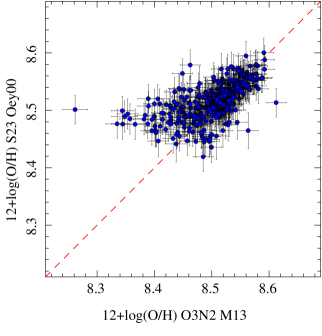
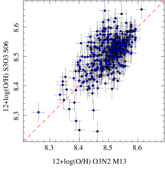
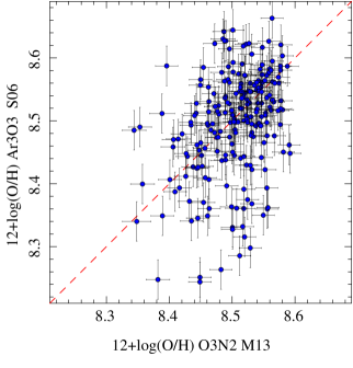
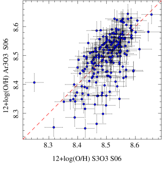
Figure 5: Comparison among the oxygen abundances derived using the different indicators described in the text: (i) S23 vs. O3N2 (top lefthand panel); (ii) S3O3 vs. O3N2 (top righthand panel); (iii) ArO3 vs. O3N2 (bottom lefthand panel); and (iv) ArO3 vs. S3O3 (bottom righthand panel). Each blue solid circle corresponds to an individual H ii region in the sample. The error bars represent half of the estimated error considering the propagation of the emission line errors and the uncertainty in the calibrator. The dashed-line corresponds in each panel to the one-to-one relation.

3.5 Oxygen abundance of H ii regions

Accurate abundance measurements for the ionized gas in galaxies require the determination of the electron temperature (T_e), usually obtained from the ratio of auroral to nebular line intensities (e.g. Osterbrock, 1989). It is well known that this procedure is difficult to carry out for metal-rich galaxies, since as the metallicity increases the electron temperature decreases (as the cooling is via metal lines), and the auroral lines eventually become too faint to measure. Therefore, calibrators based on strong emission lines are used.

Strong-line indicators have the obvious advantage of using emission lines with higher signal-to-noise, detected in mostly all H ii regions, and with large dynamical ranges. However, they have the disadvantange that the line ratios considered do not trace only the oxygen abundance, but also depend on other properties of the ionized nebulae, like the electron density, and geometrical factors, and/or the shape of the ionizing radiation (normally parametrized by the ionization parameter, $q$, or $u=q/c$ in its dimensionless form). It is well known that some of these parameters are correlated, like the trend between oxygen abundance and the ionization parameter, uncovered by the seminal studies by Evans & Dopita (1985); Dopita & Evans (1986), and recently revisited by Sánchez et al. (2014a).

There are two main schools in the derivation of oxygen abundance using strong-line indicators. One uses empirical calibrators based on the comparison of different of strong emission line ratios, with the corresponding abundance derived for a set of H ii regions for which T_e is known. The line ratios in these methods are:

$${\rm R23} = \frac{I([@series{\mathbf{O\,\mathsc{iii}}}]\leavevmode\nobreak\ \lambda\lambda 5007,4959)+I([@series{\mathbf{O\,\mathsc{iii}}}]\leavevmode\nobreak\ \lambda 3727)}{I({\rm H}\beta)}$$ (2)

$${\rm O3N2} = \frac{I([@series{\mathbf{O\,\mathsc{iii}}}]\leavevmode\nobreak\ \lambda 5007)/I({\rm H}\beta)}{I([@series{\mathbf{N\,\mathsc{ii}}}]\leavevmode\nobreak\ \lambda 6584)/I({\rm H}\alpha)}$$ (3)

$${\rm N2O2} = \frac{I([@series{\mathbf{N\,\mathsc{ii}}}]\leavevmode\nobreak\ \lambda 6584)}{I([@series{\mathbf{O\,\mathsc{ii}}}]\leavevmode\nobreak\ \lambda 3727)}$$ (4)

$${\rm N2} = \frac{I([@series{\mathbf{N\,\mathsc{ii}}}]\leavevmode\nobreak\ \lambda 6584)}{I(H\alpha)}.$$ (5)

This school adopts in most cases emission line ratios that present little or no dependence with the dust attenuation (i.e., not far in wavelength), that uses the strongest available emission lines, and calibrators that present either a monotonic or even a linear dependence with the abundance. For example, the O3N2 and the N2 indicators (Alloin et al., 1979; Pettini & Pagel, 2004; Stasińska et al., 2006; Marino et al., 2013). In some cases they use a combination of all the available emission lines, like the counterpart-method described by Pilyugin et al. (2012), or more complex combinations of non-linear equations to derive the abundances (e.g. Pilyugin et al., 2010; Pérez-Montero, 2014). Since they adopted empirical correlations, the intrinsic dependences with other parameters, like $u$, are subsummed in the calibrator by construction.

A second school prefers to use photoionization models to derive the dependence of the abundance and ionization strength with the different line ratios (e.g. Dopita et al., 2000; Kewley et al., 2001). A certain model for the ionizing stellar population is assumed, taking into account a certain burst of star formation, an initial mass function, a certain metallicity and, in some cases, the age of the cluster. Under certain conditions for the ionized nebulae (e.g., geometry, electron density), it is possible to derive trends and correlations between the abundance and the line ratios considered. For this school, the prefered line ratios are those that depend only of one of the parameters, or for which the correction on the other is well understood. The procedure/prescriptions described by Kewley & Dopita (2002) or López-Sánchez et al. (2012) on how to derive the abundances is a good example of this approach.

The main difference between the two schools is that for the first one the abundances derived are systematically lower. Dopita et al. (2014) studied a scenario in which the introduction of a $\kappa$ distribution for the electron temperatures in the nebula allows to reconcile both estimates of the oxygen abundance, based on the early studies by Binette et al. (2009). However, most of the followers of the first school still consider that the T_e or direct method is more representative of the physical conditions in the nebulae, and requires fewer assumptions or dependences on still not well understood physical properties (like the amount of ionizing photons of young stars, that differs among the different stellar evolution models). Another criticism is that in many cases the calibrations based on photoionization models assume tight or fixed correlations between the abundance of different elements (like the N/O ratio), that may affect their derived values (e.g. Pérez-Montero, 2014).

We adopted the indicator based on the O3N2 ratio described before, in order to compare with previous results on the same field. This line ratio involves the stronger emission lines in the wavelength range, as clearly appreciated in Fig. 3, and therefore minimize the errors due to the inaccuracies in the measurement of the involved line ratios. By construction, it presents a weak dependence on dust attenuation, already noticed by previous authors (e.g. Kewley & Dopita, 2002). We adopted the recently updated calibration by Marino et al. (2013), that uses the largest sample of H ii regions with abundances derived using the direct, T_e-based, method (M13 hereafter). This calibration corrects the one proposed by Pettini & Pagel (2004), that (due to the lack of H ii regions in the upper abundance range) combined direct measurements for the lower abundance range and values derived from photoionization models for the more metal rich ones. As demonstrated by Marino et al. (2013), it produces abundance values very similar to the ones estimated based on the Pilyugin et al. (2012) method, with an accuracy better than $\pm$0.08 dex.

The wavelength range covered by MUSE at the redshift of the galaxy does not include the [O ii]$\lambda$3727 emission line. Therefore, all indicators that include it, like R23, N2O2, or the combination of any of them, can not be used. However, there are other less common abundance indicators covered in this wavelength range, such as:

$${\rm S23} = \frac{I([@series{\mathbf{S\,\mathsc{iii}}}]\leavevmode\nobreak\ \lambda\lambda 9069,9532)+I([@series{\mathbf{S\,\mathsc{ii}}}]\leavevmode\nobreak\ \lambda 6717,6731)}{I({\rm H}\beta)}$$ (6)

$${\rm S3O3} = \frac{I([@series{\mathbf{S\,\mathsc{iii}}}]\leavevmode\nobreak\ \lambda\lambda 9069)}{I([@series{\mathbf{O\,\mathsc{iii}}}]\leavevmode\nobreak\ \lambda 5007)}$$ (7)

$${\rm Ar3O3} = \frac{I([@series{\mathbf{Ar\,\mathsc{iii}}}]\leavevmode\nobreak\ \lambda\lambda 7135)}{I([@series{\mathbf{O\,\mathsc{iii}}}]\leavevmode\nobreak\ \lambda 5007)}.$$ (8)

The S23 indicator was first proposed by Díaz & Pérez-Montero (2000) as an alternative to the more widely used R23. Its main advantages are that the intensity of the lines are less affected by dust attenuation, that it presents a monotonic linear dependence with the abundance for a wide range of metallicities, and that it seems to be less dependent on the ionization parameter. This later statement was questioned by Kewley & Dopita (2002) on the basis of photoionization models. Oey & Shields (2000) already noticed that this indicator has a bi-valued behaivour with respect to the abundance, similar to R23, and restricted the use of the calibrator proposed by Díaz & Pérez-Montero (2000) to subsolar metallicities ($Z<0.5Z_{\cdot}$). This corresponds to an oxygen abundance of 12+log(O/H)$<$8.3, lower than the lowest abundances derived for the H ii regions discussed here based on the M13 calibrator.

There is no published calibration of the dependence of S23 with the oxygen abundance for the higher abundance branch. However, based on the photoionization models presented by Oey & Shields (2000), it is possible to derive an estimation of the abundance for that range:

$${\rm 12+log(O/H)}=8.6-0.25{\rm log}({\rm S23})$$ (9)

The accuracy of this calibrator has to be tested extensively, but based on the range of values covered by the described models we estimate to be not better than 0.15 dex.

The S3O3 and Ar3O3 indicators were proposed by Stasińska (2006) (S06 hereafter). She derived a non-linear correlation for both indicators and the oxygen abundance, that we adopt here. She estimated the accuracy of this calibrator to be of the order of $\sim$0.09 dex.

In contrast with the O3N2 abundance indicator, that is basically independent of dust attenuation, all these indicators involve ratios of emission lines widely separated in wavelength, and therefore the line intensities must be corrected for dust attenuation prior to derive the corresponding ratio and abundance. This introduces a new degree of uncertainty that we avoid by adopting the O3N2 calibrator.

Figure 5 shows the comparison among the different estimators for the oxygen abundance discussed. We consider only the emission lines and line ratios detected above a 5$\sigma$ detection limit. Hence, each panel shows a different number of H ii regions, ranging between 210 (for the panels involving the ArO3 indicator), and 360 (for the panels involving the O3N2, S23 and S3O3 indicators). This is because the [Ar iii] emission line is fainter than any of the other (Fig.3). There is very good agreement between the different estimators, despite the different ions involved in most of the calibrators, and the inhomogenous derivation of the calibrators. The largest differences are found in the calibrator involving the [Ar iii] emission line, for the reason indicated before: $\sigma(X_{\rm O3N2}-X_{\rm Ar3O3})=0.08$ and $\sigma(X_{\rm S3O3}-X_{\rm Ar3O3})=0.07$ dex, where $\sigma$ is the standard deviation of the difference between the two estimations of the abundance, and $X$ is the oxygen abundance, i.e., 12+log(O/H). The smallest differences are found between the O3N2 and S23 indicators, with $\sigma(X_{\rm O3N2}-X_{\rm S23})=0.04$ dex, a value smaller than the expected accuracies of both calibrators. In summary, this comparison shows that our estimation of the oxygen abundance does not depend strongly on the adopted indicator, and that in average the accuracy of our estimation is of the order or better than $\sim$0.05 dex. This systematic error has been included in the error budget of the abundances derived for each individual H ii region.

3.6 Structural parameters of the galaxy

We derive the mean position angle, ellipticity, and effective radius of the disk, by a surface brightness and morphological analysis performed on the MUSE data using a V-band image of NGC 6754 synthetized from the IFS cube. The procedure is extensively described in Sánchez et al. (2014b). In summary, an isophotal analysis is performed using the ellipse_isophot_seg.pl tool included in the HIIexplorer package. Unlike other tools, like ellipse included in IRAF, this tool does not assume a priori a certain parametric shape for the isophotal distributions. The following procedures were followed for the V-band image: (i) the peak intensity emission within a certain distance of a user defined center of the galaxy was derived. Then, any region around a peak emission above a certain percentage of the galaxy intensity peak is masked, which effectively masks the brightest foreground stars; (ii) once the peak intensity is derived, the image is segmented in consecutive levels following a logarithmic scale from this peak value; (iii) once the image is segmented in $n_{levels}$ isophotal regions, for each of them, a set of structural parameters was derived, including the mean flux intensity and the corresponding standard deviation, the semi-major and semi-minor axis lengths, the ellipticity, the position-angle, and the barycenter coordinates. The median values of the derived position angles and ellipticities along the different isophotes, once excluded those affected by the seeing in the very central regions, are adopted as the position angle and ellipticity of the galaxy. Their standard deviations are considered as an estimation of the error in the derivation of these parameters. We derive an ellipticity of $e=$0.88$\pm$0.07 and a position angle of ${\rm PA}=$77$\pm$9^∘. Assuming an intrinsic ellipticity for the galaxy of $\sim$0.13 (Giovanelli et al., 1995, 1997), the inclination is estimated to be $i=$64$\pm$6^∘. Finally, we fit the surface brightness profile with a single exponential function to derive the disk scale-length, and the correponding disk effective radius, as defined by Sánchez et al. (2014b). The effective radius derived at the distance of the galaxy was estimated as $r_{e}=$10.7$\pm$0.9 kpc .

4 Results

4.1 Oxygen abundance gradient

We deproject the position of each H ii region using the morphological parameters described in the previous section. Then, we derive the galactocentric radial distribution of the oxygen abundance for NGC 6754, based on the abundances measured for each individual H ii region. For the 396 H ii regions detected, figure 6 shows the abundance gradient derived out to $\sim$2 $r_{e}$ along the galactocentric distance normalized to the effective radius.

The shape of the abundance gradient shown in this figure is totally consistent with the pattern found in many previous studies. The gradient shows an almost linear decrease between $\sim$0.3 and $\sim$1.7 effective radius, with a drop in the central regions and a flattenning and/or up-turn in the outer regions. The linear regime has been interpreted as evidence of inside-out growth in spiral galaxies, with a metal enrichment dominated by local processes (e.g., Sánchez et al., 2014b, and references therein). The drop in the inner region is found in a fraction of the spiral galaxies. In some cases (e.g., NGC 628) it has been associated with a circumnuclear ring of star formation at the expected location of the inner Lindblad resonance radius, where the gas is indeed expected to accumulate, due to non-circular motions exerted by a bar or spiral arms (Sánchez et al., 2011; Rosales-Ortega et al., 2011). The nature of the flattening in the outer regions, that has also been observed in other galaxies (e.g., Marino et al., 2012), is still under debate. It could be an effect of the radial migration of stars that latter pollute the surrounding gas, or a consequence of a change in the star-formation efficiency.

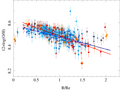
Figure 6: Radial distribution for the oxygen abundance derived using the O3N2 indicator for the 396 H ii regions detected in NGC 6754, color coded by the equivalent width of H$\alpha$. The blue colors and small symbols correspond to H ii regions with an emission EW(H$\alpha$) lower than 20Å, while the reddish-to-grey colors and larger symbols correspond to regions with higher values. The error-bars illustrate the individual errors of the abundance propagated from the estimated errors of the emission lines, not including the systematic error of the abundance calibrator. The dashed-dotted black line shows the result of the best linear regression to all the points. The blue and red solid lines correspond to the results of the best linear regressions to the H ii regions of lower and higher values of EW(H$\alpha$).

The dashed-dotted black line in Fig. 6 shows the error-weighted linear fit to this radial distribution of the abundance. Following Sánchez et al. (2014b), the analysis is restricted to galactocentric distances 0.3$<r/r_{e}<$2.1. We find a slope in the abundance gradient of $\alpha$=$-$0.10$\pm$0.02 dex/$r_{e}$, which is similar to the common abundance slope reported by Sánchez et al. (2014b) of $\sim$$-$0.1 dex/$r_{e}$. If we used the same calibrator than the one adopted in that study, i.e., Pettini & Pagel (2004), instead of Marino et al. (2013), the slope would be slightly larger, $\alpha$=$-$0.14$\pm$0.02 dex/$r_{e}$. In any case, both slopes are totally compatible with the common gradient, since they are both within 1$\sigma$ of the range of values described for this characteristic slope (Sánchez et al., 2014b).

The number of H ii regions detected for this galaxy is large enough to explore whether the abundance gradient depends on other properties of the nebular emission. The H ii regions in Fig. 6 have been color-coded according to the value of the EW(${H\alpha}$). Adopting this scheme it is possible to distinguish between the regions with stronger specific star-formation rate, that trace mostly the spiral arms (Fig. 1), and those distributed more homogeneously across the entire disk. We repeat the fitting procedure splitting the sample in two, for H ii regions with equivalent width greater or smaller than 20Å. We find that the H ii regions with lower equivalent widths present a somewhat shallower gradient ($\alpha$=$-$0.09$\pm$0.01) than those with higher equivalent widths ($\alpha$=$-$0.12$\pm$0.02). The two gradients are shown in Fig. 6. However, the difference is rather small, and it may not be significant. In order to test it, we perform a Kolmogorov-Smirnov (KS) test to estimate how different the distributions of oxygen abundances in both cases are. We find that the probability that both distributions were not derived from the same sample is just a 7.7%. Therefore, there is no significant difference between the abundance gradients for the regions with stronger or fainter specific star formation rates.

We explore possible differences in the abundance gradients based on other properties of the ionized nebulae. First, we considered the ionization parameter, splitting the sample in two subsamples with log(u) greater or smaller than $-$3.6 (the median value for our sample). The differences in the slopes were even smaller, being $\alpha_{highlog(u)}=-$0.10$\pm$0.02 dex and $\alpha_{lowlog(u)}=-$0.08$\pm$0.03 dex. Then, we considered the electron density, splitting the sample in regions with $n_{e}$ greater or smaller than 75 cm^-3 (the median value for our sample). In this case we find the same slope for both subsamples ($\alpha_{highn_{e}}=-$0.10$\pm$0.03 dex).

Finally, we explore if the different spatial resolutions of the east and west pointings have an impact in the abundance distributions and gradients. We repeat the analysis restricting our sample to the regions detected in both pointings separately before joining them into a single catalog. We find very similar slopes for both subsamples: $\alpha_{east}=-$0.10$\pm$0.02 dex and $\alpha_{west}=-$0.12$\pm$0.03 dex. Even more, a KS-test indicates that the probability that both distributions were not derived from the sample sample is 0.02%.

4.2 Mixing scale-length

This sample of H ii regions is large enough to derive a estimation of the mixing scale-length. For doing so we compute the dispersion of galactocentric distances with respect to the linear regression. The average of this relative distance is zero (by construction), and the standard deviation is the typical mixing scale, i.e., how far a certain H ii region has moved from its expected location based on a pure inside-out chemical enrichment without radial mixing. We find a mixing scale-length $r_{mix}=$0.43$r_{e}$, that corresponds to 4.6 kpc at the redshift of this galaxy.

We repeated the estimation for the different sub-samples of H ii regions discussed before, and found similar dispersions, covering a range of values of $r_{mix}=$0.37$-$0.53$r_{e}$. In particular, when taking into account the east and west pointing separately we derive a very similar radial mixing scale-length, slightly lower than the common one ($r_{mix,east/west}=$0.35$r_{e}$). This indicates that (i) the different spatial resolution does not affect the result, and (ii) there seems to be an azimuthal variation of the oxygen abundances that increases the dispersion when not taken into account. Finally, we study if there is a dependence with galactocentric distance. We found that the mixing scale-length is slightly lower in the inner regions $r_{mix}(r/re<0.9)=$0.28$r_{e}$ than in the outer ones $r_{mix}(r/re>0.9)=$0.67$r_{e}$.

To know how sensitive this dispersion is to the errors and uncertainties in the derived parameter, we performed a simple Monte-Carlo simulation, allowing each of the parameters (abundances, galactocentric distances, effective radius and inclination) to vary within the estimated errors. The standard deviation between the different estimated radial mixing scales is $\sim$0.15$r_{e}$.

This parameter puts a strong constraint on the metal mixing scale-length, independently of the mechanism required to produce the mixing. Obviously this is an upper limit to the mixing scale-length, in particular if the abundance gradient depends on the equivalent width of H$\alpha$.

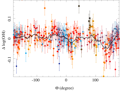
Figure 7: Azimuthal distribution of the residual of the oxygen abundance for the individual H ii regions once subtracted the average radial gradient. The colors and sizes indicate the galactocentric distance, with blue solid circles corresponding to H ii regions more nearer to the center of the galaxy, and red/orange ones corresponding to those farther away. The solid line corresponds to the average value at each azimuthal angle for H ii regions within 25^∘of the considered angle.

4.3 Azimuthal variations of the oxygen abundance

In a pure inside-out scenario where the metal enrichment is dominated by local processes (the metal pollution by stars that dies at a certain location), the abundance gradient should not present any azimuthal variation. Different mechanisms proposed for the radial mixing predict different characteristic patterns in the azimuthal distribution of the oxygen abundance. The sample of H ii regions provided by our MUSE data is large enough to explore if there is an azimuthal variation in the distribution of oxygen abundances.

Figure 7 shows the azimuthal distribution of the oxygen abundances for the H ii regions of our catalog, once removed the common radial gradient, for those regions within a ring of 0.3$<r/r_{e}<$2.1 (i.e., the linear regime of the abundance gradient). There is a clear pattern, more clear when we derive the azimuthal average within a box of 25^∘around each value. Indeed, when removing this average pattern the dispersion around the mean value is reduced by a 40%. The amplitud of the pattern does not follow a clear periodic sequence (like a sinusoidal structure), and there is no clear general dependence with the galactocentric distance.

However, in the strongest feature of this pattern, the wiggle between $\theta\sim$90^∘and $\theta\sim$160^∘with an amplitude of $\sim$0.05 dex, there seems to be a trend with distance, with the abundance decreasing at intermediate distances and increasing for both the inner and outer regions. This pattern corresponds to the spiral arm the south-east of the center of the galaxy. If real, this could be a hint of radial mixing.

The radial mixing scale defined in the previous section is reduced to 0.39$r/re$, or 4.1kpc, when the average azimuthal variation of the oxygen abundance is subtracted prior to derive the dispersion around the radial abundance gradient.

5 Discussion and Conclusions

In this study we analyse one of the first observations using MUSE on a spiral galaxy, NGC 6754. We detect and extract the spectroscopic information of a sample of 396 H ii regions, an order of magnitude larger than the average number observed in previous state-of-the-art IFU survey datasets (e.g. Sánchez et al., 2014b). This illustrates the capabilities of this unique instrument due to the combination of its large FoV and unprecedent spatial sampling/resolution.

The abundance distribution derived has a negative gradient, with a slope consistent with the characteristic value reported by previous studies (Sánchez et al., 2014b), in the linear regime between 0.3 and 1.7 $r_{e}$. The abundance decreases in the inner regions, and there is a hint of a flatenning in the outer parts. Both features have been already observed in previous studies in individual galaxies (e.g., Bresolin et al., 2009; Yoachim et al., 2010; Rosales-Ortega et al., 2011; Marino et al., 2012; Bresolin et al., 2012). The central drop is in many cases associated with a circumnuclear star-formation process (Sánchez et al., 2014b), and it could be related with the accumulation of gas due to non-circular motions exerted near the inner Lindblad resonance radius (e.g., Cepa & Beckman, 1990).

The nature of the flatenning is still not clear. A detailed discussion on the different scenarios proposed was presented by Sánchez et al. (2014b). In summary, under the usually observed star-formation rates, the time required to enrich the ISM up to the observed abundances in these outer regions is of the order of the age of the Universe (Bresolin et al., 2012), and therefore it is unlikely that in situ star-formation could have enriched the interstellar medium to the values observed. Among the main mechanisms proposed to explain the flatenning we highlight the following ones: (i) angular momemtum transport that produces a radial mixing (e.g., Lacey & Fall, 1985b; Goetz & Koeppen, 1992; Portinari & Chiosi, 2000; Schönrich & Binney, 2009; Spitoni & Matteucci, 2011); (ii) resonance scattering with transient spiral density waves (Sellwood & Binney, 2002a); (iii) the overlap of spiral and bar resonances (Minchev et al., 2011); (iv) stellar radial migration (e.g., Roškar et al., 2008b, a); and (v) minor mergers and captures of satellite galaxies (Quillen et al., 2009; Bird et al., 2012).

We explore the possible dependence of the slope of the abundance gradient with different properties of the ionized gas. Significant differences are not expected if the metal enrichment is dominated by the inside-out growth of the galaxy. However, local processes, like outflows or metal raining induced by enhanced star-formation associated with the spiral arms may modify the chemical distribution locally. Under this assumption it would be expected that denser H ii regions in spiral arms, with greater EW($H\alpha$) , and ionization strengths present a different distribution of oxygen abundances that those H ii regions located in the inter-arm regions. Our results indicate that local processes do not seem to be relevant enough to modify the galactocentric abundance gradient in this particular galaxy.

We define a parameter to estimate the amount of the redistribution of metals within the galaxy that we call the mixing scale-length, $r_{mix}$. This parameter is defined as the dispersion around the abundance gradient along the galactocentric distance, and can be derived as the ratio between the dispersion in the abundance and the slope of the correlation. We estimate the typical $r_{mix}=$0.43$\pm$0.15 $r_{e}$, i.e., $\sim$4.6 kpc at the redshift of the galaxy. To our knowledge, this is the first time that this parameter is defined in this way. However, it is possible to compare with previous results if both the dispersion in abundance and the slope of the radial gradient are provided. The most recent exploration of the abundance gradient over a large sample of galaxies was published by Sánchez et al. (2012b, 2014b). They found that the common abundance gradient has a slope of $\alpha=-$0.1 dex/$r_{e}$, with a dispersion of $\sim$0.6 dex, for which an average mixing scale-length of $r_{mix}\sim$0.6 $r_{e}$ is derived. This value is slightly larger than the one we find for NGC 6754. However, we should note here that the estimation derived from Sánchez et al. (2012b, 2014b) results is purely statistical, based on the average abundance gradient derived once the individual gradients for each galaxy are considered all together and normalized to the abundance at the effective radius. Measurements on individual galaxies have not been provided.

Bars have been proposed as an effective mechanism for radial migration (e.g., Athanassoula, 1992; Sellwood & Binney, 2002b). Hydrodynamical simulations have shown that bars induce angular momentum transfer via gravitational torques, that result in radial flows and mixing of both stars and gas (e.g., Athanassoula, 1992). These radial motions can produce a mixing and homogenization of the gas, that leads to a flattening of any abundance gradient (e.g., Friedli, 1998). Resonances between the bar and the spiral pattern speeds can shift the orbits of stars, mostly towards the outer regions (Minchev & Famaey, 2010), a mechanism that also affects the gas. Another process that produces a similar effect is the coupling between the pattern speed of the spiral arms and the bar, that induces angular momentum transfer at the corotation radius (e.g., Sellwood & Binney, 2002b). In a recent study Di Matteo et al. (2013) analysed the signatures of radial migration in barred galaxies on the basis of simulations. They found that the slope of the abundance gradient does not change significantly up to $\sim$1.5-2 $r_{e}$ (when the scale-length of their simulated disks are transformed to an effective radius), but a flatenning is predicted beyond these galactocentric distances. This pattern is very similar to the one observed in our galaxy. However, as we discussed before, the flatenning in the outer region seems to be present in spiral galaxies irrespective of the presence or absence of bars (Sánchez et al., 2014b).

Di Matteo et al. (2013) defined a parameter to quantify the amount of spatial redistribution of stars in a disk as the ratio between the maximum absolute variation of the metallicity with respect to the radial gradient compared to the slope of this gradient ($\delta_{[Fe/H]}/\Delta_{[Fe/H]}$). With units of distance, this parameter is equivalent to our mixing scale-length ($r_{mix}$). They found that this parameter evolves with time and presents a weak radial dependence. At the peak of the radial migration it ranges between 1-1.5 kpc (0.17-0.26 $r_{e}$) for a galactocentric distance between 3 and 12 kpc (0.5-2 $r_{e}$). As time evolves it decreases, being slightly larger in the outer regions. Our derived $r_{mix}$ is larger, but certainly of the same order, than that predicted by Di Matteo et al. (2013). It also presents a weak radial dependence, that may indicate that the peak of the migration has already past. This is a good agreement considering that we are not comparing with ad hoc simulations specifically done to reproduce our galaxy.

Another prediction by simulations is that the radial mixing should not be homogeneous. These inhomogeneities are related to the way radial migration occurs in galaxies, following the arms pattern (e.g., Minchev et al., 2012): metal-rich stars which move to the outer disk are mostly from the region outside corotation (Brunetti et al., 2011), and migrate through spiral patterns to the outer parts of the disk. In other words, migration is not axisymmetric, but associated to the distribution of arms and bars. In Section 4.3 we explored the possible azimuthal variations of the oxygen abundance, once subtracted the radial dependence, and we found evidence of an asymmetrical distribution. The strongest feature is associated with the spiral arms in the south-east of the galaxy. The amplitude seems to be smaller than that predicted by Di Matteo et al. (2013), for the epoch of the strongest migration: $\sim$0.2 dex at $\sim$7 kpc (1 $r_{e}$), at t=1.1 Gyr in their simulations (Fig. 8, top panel, in that article). However, this effect is expected to become weaker with time (Figure 8, bottom panel of that article), and our previous result indicates that this galaxy has already passed the peak of the strongest migration.

The proposed scenario assumes that the deviation of the abundances with respect to the radial gradient, due to the radial migration associated with arms and bars, should be stronger in barred galaxies. This is a consequence of the stronger radial movements expected to be induced by these morphological features. In this context it is interesting to note that recent results indicate that the stellar and gas kinematics of barred and un-barred galaxies seem to be very similar, without stronger distorsions induced by the presence of the bar, at least at large scales Barrera-Ballesteros et al. (2014).

Despite the fact of this significant advance in our understanding of the possible effects of radial mixing, it is important to highlight that all these results were derived for a single galaxy. Larger samples of galaxies are needed to explore whether the estimated mixing scale-lengths and azimuthal variations depend on other properties of the galaxies, such as the presence or absence of bars, the strength of the bars, the interaction stage, the morphological type, and the stellar mass or luminosity. In particular, if the picture outlined by Di Matteo et al. (2013) is valid, we should find different strengths in both $r_{mix}$ and the intensity of the azimuthal variations depending on the timing of the evolution of the bars and the coupling or not with the spiral arms. Another important caveat is that the results from the current simulations were focused on the effects of the migration on old stars, and in their metallicities. As clearly illustrated in recent results by González Delgado et al. (2014) the gas-phase abundance is better correlated with the metallicity of young stars ($t<$2 Gyr), with old stars being in general more metal poor. It is still unclear how these differences may affect the interpretation of our results on the basis of the simulations. However, there is a lack of similar simulations on the effects of radial migration for the gas-phase abundance.

The current results illustrate the capabilities of MUSE to accomplish this kind of studies in a very efficient way, and demonstrate that it is possible to derive reliable dispersions around the mean abundance gradient. In future articles we will apply the methodology outlined here to a sample of galaxies with similar characteristics of cosmological distances and projected sizes, observed with this instrument, in order to explore the dependence of the results on galaxy type, as outlined before.