General three-state model with biased population replacement:
Analytical solution and application to language dynamics

Abstract

Empirical evidence shows that the rate of irregular usage of English verbs exhibits discontinuity as a function of their frequency: the most frequent verbs tend to be totally irregular. We aim to qualitatively understand the origin of this feature by studying simple agent–based models of language dynamics, where each agent adopts an inflectional state for a verb and may change it upon interaction with other agents. At the same time, agents are replaced at some rate by new agents adopting the regular form. In models with only two inflectional states (regular and irregular), we observe that either all verbs regularize irrespective of their frequency, or a continuous transition occurs between a low-frequency state where the lemma becomes fully regular, and a high frequency one where both forms coexist. Introducing a third (mixed) state, wherein agents may use either form, we find that a third, qualitatively different behavior may emerge, namely, a discontinuous transition in frequency. We introduce and solve analytically a very general class of three–state models that allows us to fully understand these behaviors in a unified framework. Realistic sets of interaction rules, including the well-known Naming Game (NG) model, result in a discontinuous transition, in agreement with recent empirical findings. We also point out that the distinction between speaker and hearer in the interaction has no effect on the collective behavior. The results for the general three–state model, although discussed in terms of language dynamics, are widely applicable.

I Introduction

Language is structured by rules Hockett (1961); Chomsky (1986) - but linguistic rules often have exceptions. This fact kindled a long-standing debate in cognitive science centering on how individual learners accommodate rule sets rife with exceptions (e.g., see Refs. Pinker (1999); McClelland and Patterson (2002)). However, how exceptions arise and evolve over time within a language system remains a largely open question.

The study of the English past tense is widely used as an exemplar of the interplay between rules and exceptions Pinker and Ullman (2002); Bybee and Slobin (1982a); Marslen-Wilson and Tyler (1998); Plunkett and Marchman (1996). A recent study of historical corpus data Cuskley et al. (2014a) looks at rules in the language system rather than individual learners, shedding light on the relationship between the verb frequency and regularity (Fig. 1).

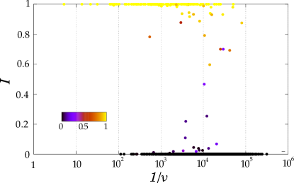
Figure 1: (color online) Plot of $I$, the fraction of times a verb is used in the irregular past tense form as a function of the inverse of its frequency of usage $\nu$, for 2840 english verbs in the CoHA corpus for the decade 1980-1989. The color (shade) of each symbol represents the average value of $I$ across 16 decades between 1830 and 1989. (Adapted from Ref. Cuskley et al. (2014a)).

Each verb in the language can be characterized by $I$, the fraction of irregular past tense tokens over the total number of tokens in the past tense, and $\nu$, its frequency of usage. An interesting transition is found in the behavior of $I$ as a function of $\nu$: regular verbs dominate the low frequency range, while most irregular verbs are located at higher frequencies (see also Refs. Lieberman et al. (2007); Carroll et al. (2012)). For intermediate values of $\nu$ fully regular ($I=0$) and fully irregular ($I=1$) verbs coexist. Only a small subset of verbs exhibit both regular and irregular forms ($0<I<1$), and occur primarily in a rather narrow range of frequencies between the dominant regular and irregular states.

The work presented in this paper takes a theoretical approach to the relationship between rules and exceptions in a population of interacting speakers. We investigate the dynamics of a set of very simple agent-based models aimed at describing the fundamental mechanisms by which rules and exceptions may be shared or disappear in a population, in the same spirit of the Naming Game (NG) Baronchelli et al. (2008); Loreto et al. (2011) investigations of the emergence of shared naming conventions. We consider a single lemma and examine two-state and three-state models. In a two-state model, an individual has an internal inflectional inventory which can contain either the regular (R) or irregular (I) inflection for the lemma. In a three-state model, the inflectional state can be either R, I or mixed (M). The mixed state represents intra-speaker variation Labov (1972), where an individual may accommodate both regular and irregular forms for a single word Dale and Lupyan (2012). For example, there is evidence that regular and irregular past tense verb forms are simultaneously known and potentially used in seemingly free variation within a single speaker (e.g., both sneaked and snuck are acceptable Dale and Lupyan (2012)). Agents are endowed at the start of the dynamics with some inflectional state for the word and engage at rate $\nu$ in pairwise interactions, i.e. one of them utters the verb under consideration and the other listens to it. During interaction, the inflectional states of the speaker and hearer change according to a pre-defined set of interaction rules. In addition to interaction events, we implement a replacement mechanism: at rate $r$ an agent is replaced with a “child” who engages in overregularization: these “child” agents assume the regular inflection applies to all words in the vocabulary, representing a known bias of child learners, Berman (1981); Bybee and Slobin (1982b); Maslen et al. (2004). Replacement represents turnover in the population: as a child learner enters, an adult leaves (i.e., is replaced), so that the population size remains constant.

We first approach some specific models analytically, within the framework of mean-field theory. This analytical approach allows for quantitative predictions regarding which state a population of speakers will reach given a particular set of interaction rules and the type of transition which may occur depending on the ratio between the frequency and replacement rates. It turns out that different interaction rules lead to qualitatively different types of behavior. Two-state models lead to total regularization or to a continuous transition as a function of $r/\nu$. Three-state models, on the other hand, have the potential to exhibit a discontinuous transition with some highly frequent, mostly irregular words, reminiscent of findings in empirical data. To understand these variations and understand their origin, we introduce a very general three-state model, encompassing all possible sets of interaction rules that do not favour either the regular or irregular state in their outcome. We provide a formal solution for any value of the model parameters and study in detail the conditions under which no transition (i.e., total regularization) occurs, and the conditions under which we observe a continuous or discontinuous transition. Our analysis also shows that assuming asymmetric influence of the speaker over the hearer in the interaction has no effect on the collective behavior. The results for this general model are discussed in terms of language dynamics, but their applicability is fully general: they give the solution for any three-state model of population dynamics with unbiased interaction rules and biased replacement.

II Two-state models

Let us start by considering two-state models, where each individual can be found in one of two possible rule states, regular (R) or irregular (I). While in this case the two states represent regular and irregular inflections, this framework can represent any set of binary options (e.g., the choice between two possible words to name an object, two alternative opinions on a given topic, etc.). As a specific example, the Abrams-Strogatz model Abrams and Strogatz (2003) used a two–state approach to examine the dynamics of endangered languages, providing a prime example of the dynamics of languages in competition more generally.

Using this general two–state model approach, we focus here on the binary options of regular (R) or irregular (I) inflection for a single word, characterized by its frequency of usage, $\nu$. At each interaction step two agents are selected at random (i.e., mixing is homogeneous) and assigned the role of either speaker or hearer. With probability $\nu$ they engage in a pairwise interaction (i.e. the speaker utters the verb under consideration to the hearer), which affects their inflectional states according to specific interaction rules. Then, with probability $r$ one individual in the population is replaced with a “child” having its inflectional state set to R. This part of the dynamics mimics the turnover of some segment of the adult population into child learners at rate $r$, keeping the population size $N$ fixed, and assuming over-regularization behavior in new learners. In this way the population replacement is biased towards one of the two options, in this case, regularity. The quantity $1/r$ can be interpreted as the life expectancy of an individual in the population.

Among the possible two–state interaction rules, we consider the sets presented in Table 1.

Before			After
			Model A:			Model B:			Model C:
			Irregular-biased			Regular-biased			Speaker leads
Speaker	Hearer		Speaker	Hearer		Speaker	Hearer		Speaker	Hearer
R	R		R	R		R	R		R	R
R	I		I	I		R	R		R	R
I	R		I	I		R	R		I	I
I	I		I	I		I	I		I	I

Table 1: Interaction rules for the two-state models. The two columns on the left refer to the status of speaker and hearer prior to interaction. The next three pairs of columns refer to the status of speaker and hearer after the interaction in the three models.

In the Irregular–biased (A) and Regular–biased (B) models, the speaker and the hearer roles are symmetric; in other words, which agent identifies as speaker or hearer is irrelevant, but the presence of an I(R) state in the interaction leads the rules. In A(B) an agent switches to the I(R) state whenever interacting with a partner in the I(R) state, regardless of which agent is the speaker and which the hearer. In these cases the speaker can affect the hearer’s state, and the hearer can also affect the speaker’s. In the Speaker leads model (C) the roles are not symmetric: the speaker never changes its state and the hearer always adopts the state of the speaker.

The Irregular–biased model is perfectly equivalent to one of the most fundamental models of non–equilibrium statistical physics: the contact process Marro and Dickman (1999). The temporal behavior of this model is easily understood by writing down the mean-field evolution equation for the density $\rho_{I}$ of individuals in the I state (the density of R individuals, $\rho_{R}$, being trivially $1-\rho_{I}$)

$$\dot{\rho}_{I}=-r\rho_{I}+2\nu\rho_{I}(1-\rho_{I}).$$ (1)

Equation (1) is solved straightforwardly and yields, for any initial configuration $\rho_{I}(0),\rho_{R}(0)=1-\rho_{I}(0)$

$$\rho_{I}(t)=\frac{2/n-1}{2/n+\left(\frac{2/n-1}{\rho_{I}(0)}-2/n\right)e^{-r(2/n-1)t}}$$ (2)

where $n=r/\nu$.

For long time scales, the system reaches (for any initial configuration) a stationary state which exhibits a continuous transition for a critical value $n_{c}=2$, between a fully regular state ($\rho_{I}=0$) for $n>n_{c}$, and a state with individuals in both the R and the I state ($\rho_{I}>0$):

$$\rho_{I}=\left\{\begin{array}[]{lr}0&\;n\geq n_{c}\\ 1-\frac{n}{2}&0\leq n<n_{c}.\end{array}\right.$$ (3)

The solutions for the Regular–biased and Speaker leads models are obtained from Eq. (2) by simply replacing $n\rightarrow-n$ and $n\rightarrow\infty$, respectively, and both result in an exponential relaxation to the stationary fully regular state ($\rho_{I}=0$) for any physical value of $n$. Unlike in case A, in these two cases the interaction rules are biased in favor of R (case B) or unbiased (C) and they cannot compensate for the increase in R states due to replacement, leading to a fully regular absorbing state.

As it will be demonstrated in Sec. IV.1, no two-state model can give rise to a discontinuous transition between the fully regular state and a state with $\rho_{I}>0$. Empirical data, however, exhibit such a discontinuous transition, and research shows that speakers can accommodate regular and irregular forms simultaneously Dale and Lupyan (2012). For these reasons, we now turn our attention to a more complex modeling scheme that integrates a third, mixed state (M), wherein agents accommodate either the R or I. We will show that introducing this, psychologically plausible, mixed state, a qualitatively different behavior appears, namely, a discontinuous transition in regularity, reminiscent of empirical data.

III Three-state models

In three–state models there are still only two alternative inflections that can be applied to a word (R and I) during an interaction event, but internally, each individual can be in one of the three possible states: R (regular), I (irregular) and M (mixed). In the mixed state the individual can accommodate both R and I forms; this accounts for agents undecided on which is the correct form to use, or that consider both the regular and the irregular form acceptable.

The study of three-state models has a long history in the investigation of language dynamics (for a review see Castellano et al. (2009)). In particular, Wang and Minett proposed Wang and Minett (2005); Minett and Wang (2008) deterministic models for the competition of two languages, that included a third potential state of bilingual individuals. Castelló et al. Castelló et al. (2006) proposed a modified version of the voter model Clifford and Sudbury (1973); Holley and Liggett (1975) to examine language which included bilingual individuals, the so-called AB model. Synonymy, the possibility for having multiple potential names for a single meaning (much like multiple inflections for a single verb as in the mixed state) has also been examined in the classic Naming Game (NG) model Baronchelli et al. (2006, 2008). The Naming Game and its variants have examined structures of increasing complexity, often including agents who can have multiple internal states, from the categorisation of colors Puglisi et al. (2008); Mukherjee et al. (2011) to basic syntactic structures Tria et al. (2012).

We now study the dynamics of three specific examples in the class of three-state models, with different microscopic rules leading to qualitatively different behaviors (see Table 2). The first set of rules is known as the Naming Game.

Before			After
			Model NG			Model CT			Model NT
Speaker	Hearer		Speaker	Hearer		Speaker	Hearer		Speaker	Hearer
R	R		R	R		R	R		R	R
R	I		R	M		R	M		M	M
R	M		R	R		R	M		R	R
									M	M
I	R		I	M		I	M		M	M
I	I		I	I		I	I		I	I
I	M		I	I		I	M		I	I
									M	M
M	R		M	M		R	R		R	R
			R	R		I	M		M	M
M	I		I	I		I	I		I	I
			M	M		R	M		M	M
M	M		I	I		R	M		I	I
			R	R		I	M		R	R
									M	M

Table 2: Interaction rules for the three examples of three-state models. The two columns on the left refer to the status of speaker and hearer prior to the interaction. The following three pairs of columns refer to the status of speaker and hearer after the interaction for the three different rule sets: the Naming Game (NG), the Continuous Transition (CT) model and the No Transition (NT) model. When two alternative inflections are possible because of a mixed state, the probability of each of them is $1/2$. In the only case with three alternative outcomes (I,I) and (R,R) occur each with probability 1/4, while (M,M) occurs probability 1/2.

III.1 The Naming Game with biased replacement: A three–state model with a discontinuous transition

The interaction dynamics of the Naming Game with three states are as follows: first, at each time step a speaker and a hearer are selected at random. With the probability $\nu$ they interact; the speaker conveys to the hearer either the R or I form depending on his inventory (if in the mixed state he utters R or I with equal probability). If the hearer’s inventory contains the inflection used in the utterance, both agents update their inventories keeping only the form involved in the interaction. Otherwise, the hearer adds the form to his inventory (thus switching to the mixed state). Table 2 (first four columns) summarizes these interaction rules. In addition to these rules, the population turnover is implemented as in the previous two-state models: at each time step an individual is selected at random and, with probability $r$, is replaced by a new individual in state R.

In a generic three-state model, two densities are needed to specify the global state of the system. We choose $\rho_{I}$ and $\rho_{R}$, the density of the mixed state being $\rho_{M}=1-\rho_{R}-\rho_{I}$. The mean-field equations for the Naming Game with biased replacement are:

$$\left\{\begin{array}[]{lll}\dot{\rho}_{I}&=&-r\rho_{I}+\nu(1+\rho_{R}^{2}-2\rho_{R}-\rho_{I})\\ \dot{\rho}_{R}&=&r(1-\rho_{R})+\nu(1+\rho_{I}^{2}-2\rho_{I}-\rho_{R}).\end{array}\right.$$ (4)

Notice that the equations for the usual Naming Game with three states Baronchelli et al. (2007, 2008) are recovered by setting $r=0$ and $\nu=1$.

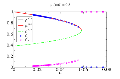
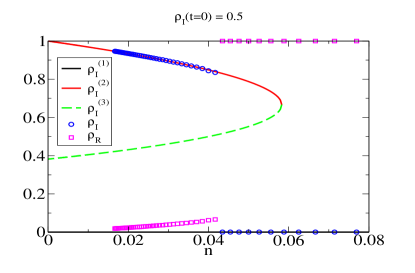
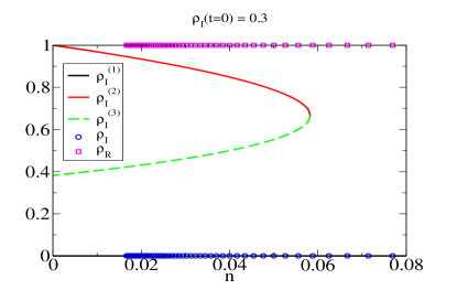
Figure 2: (color online) Phase diagram of the NG model as a function of $n=r/\nu$. The black line indicates the stationary solution $\rho_{I}^{(1)}$, while green (light gray) and red (dark gray) curves indicate solutions $\rho_{I}^{(2)}$ (stable) and $\rho_{I}^{(3)}$ (unstable), respectively. Symbols are the stationary values of the fraction of irregulars $\rho_{I}$ and regulars $\rho_{R}$ from numerical simulations with different initial conditions: from top to bottom $\rho_{I}(t=0)=0.8,0.5$ and $0.3$. The three panels show the dependence of the stationary state on the initial condition.

Imposing the stationarity condition, after some algebra one finds that the density of individuals in the irregular state is given by the fourth order equation

$$\rho_{I}\left(1+n\right)^{3}=\rho_{I}^{2}(\rho_{I}-2)^{2},$$ (5)

where $n=r/\nu$. One solution is, for any $n$, the trivial value $(\rho_{I}^{(1)},\rho_{R}^{(1)})=(0,1)$, corresponding to the fully regular state. Regarding the three other solutions, since $(1+n)^{3}$ is always larger than 1, it follows that one solution ($\rho_{I}^{(4)},\rho_{R}^{(4)}$) is always real but unphysical (being larger than 1), while the two others are complex for $n>{2\sqrt[3]{4}/3-1)}\approx 0.0583$. Below this critical value (corresponding to a saddle-node bifurcation), these two solutions are real and physical:

$$\rho_{I}^{(2)} = \frac{4}{3}\left[1+\cos\left(\frac{\cos^{-1}\left[\frac{27}{16}\left(1+n\right)^{3}-1\right]}{3}+\frac{4\pi}{3}\right)\right]$$ (6)

$$\rho_{I}^{(3)} = \frac{4}{3}\left[1+\cos\left(\frac{\cos^{-1}\left[\frac{27}{16}\left(1+n\right)^{3}-1\right]}{3}+\frac{2\pi}{3}\right)\right]$$ (7)

with the stationary value of $\rho_{R}$ given by

$$\rho_{R}^{*}=1-\sqrt{\left(1+n\right)\rho_{I}^{*}}\ .$$ (8)

For $n=0$ the solutions converge to the values found for the usual Naming Game Baronchelli et al. (2007, 2008): $(\rho_{I}^{(2)},\rho_{R}^{(2)})=(1,0)$, and $(\rho_{I}^{(3},\rho_{R}^{(3)})=((3-\sqrt{5})/2,(3-\sqrt{5})/2)).$

The physical stationary solutions are represented in Fig. 2 as a function of $n$. The stability of the generic solution $(\rho_{I}^{*},\rho_{R}^{*})$ as a function of $n$ is investigated by looking at the eigenvalues and eigenvectors of the stability matrix, defined through the equations:

$$\frac{d}{dt}\left[\begin{array}[]{cc}\delta\rho_{I}\\ \delta\rho_{R}\end{array}\right]=\left[\begin{array}[]{cc }-r-\nu&2\nu(\rho_{R}^{*}-1)\\ 2\nu(\rho_{I}^{*}-1)&-r-\nu\end{array}\right]\left[\begin{array}[]{cc}\delta\rho_{I}\\ \delta\rho_{R}\end{array}\right].$$ (9)

The eigenvalues are given by:

$$\lambda_{1,2}=\pm 2\nu\sqrt{(\rho_{I}^{*}-1)(\rho_{R}^{*}-1)}-(r+\nu).$$ (10)

Figure 3 reports the complete phase flow in the space ($\rho_{I}$, $\rho_{R}$) for $n=0$ and $n=0.025$. For $(\rho_{I}^{(1)},\rho_{R}^{(1)})=(0,1)$ both eigenvalues are negative: the fully regular state is always attractive and stable and for $n>(2\sqrt[3]{4}/3-1)\approx 0.0583$ it is the only physical solution. For $n<(2\sqrt[3]{4}/3-1)\approx 0.0583$ the two other physical solutions appear. ($\rho_{I}^{(2)}$, $\rho_{R}^{(2)}$) is always stable and attractive and, for $n>0$, it always corresponds to states for which $\rho_{I}+\rho_{R}<1$. Let us now focus on the ($\rho_{I}^{(3)}$, $\rho_{R}^{(3)}$) solution. This solution corresponds to a saddle point (the red circles in Fig. 3) since it has one positive and one negative eigenvalue. The separatrix in the attractive direction corresponds to the eigenvector associated to the negative eigenvalue:

$$\rho_{R}=\rho_{R}^{(3)}+m(\rho_{I}-\rho_{I}^{(3)})$$ (11)

with $m=\sqrt{(1-\rho_{I}^{(3)})/\sqrt{(1+n)\rho_{I}^{(3)}}}$ (the thick red solid line in the figure). The other separatrix is locally approximated in the neighborhood of ($\rho_{I}^{(3)}$, $\rho_{R}^{(3)}$), by

$$\rho_{R}=\rho_{R}^{(3)}-m(\rho_{I}-\rho_{I}^{(3)})$$ (12)

(the thin green solid line in Fig. 3). In Appendix A we report the explicit expressions for the limit case $n=0$, i.e., the original Naming Game.

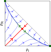
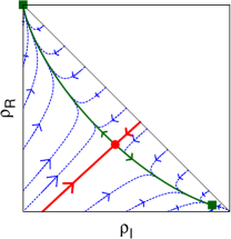
Figure 3: (color online) Phase-space ($\rho_{I}$, $\rho_{R}$) for the NG model with biased population replacement illustrating fixed points, separatrix and phase flows (represented by blue dashed lines) for (left) $n=0$ and (right) $n=0.025$. The green squares are the attractive stable solutions $(1)$ and $(2)$, while the red circles are the solution $(3)$ that correspond to a saddle point with an attractive and a repulsive direction. Only the fraction of the physical phase space with $\rho_{I}+\rho_{R}<1$ is represented.

The model exhibits a discontinuous transition between a phase (high values of $n=r/\nu$) where, whatever the initial condition, the stationary state is fully regular and a phase (low values of $n$) where both the fully regular state (solution $(1)$) and a state with a large fraction of irregulars (solution $(2)$) are stable. As depicted in Figure 3, the initial condition determines which one of the two states is asymptotically reached. In particular if the initial condition is above the separatrix corresponding to the attractive direction (thick red line) all individuals converge to the fully regular state (solution $(1)$); on the other hand if the initial condition is below that separatrix the system converges to the solution $(2)$ where a fraction $\rho_{I}^{(2)}$ ($\rho_{I}^{(2)}=1$ for the case with no replacement, $n=0$) of irregulars coexists dynamically with regular and mixed individuals. Only initial conditions exactly on the separatrix (thick red line) lead to convergence to solution $(3)$. The predictions of the MF theory are confirmed by numerical simulations of the actual agent-based model (Fig. 2).

In summary, the Naming Game with biased population replacement exhibits a discontinuous transition as a function of $n$. The discontinuity also implies a dependence of the final steady state on the initial condition which provides a theoretical justification for the observation of a range of frequencies where both fully regular and mostly irregular verbs exist (see Fig. 1). For every frequency in this interval, verbs will converge to the fully regular state $(1)$ or to the mostly irregular state $(2)$, depending on the initial values of $\rho_{R}$ and $\rho_{I}$. This phenomenology is in agreement the empirical findings reported in Cuskley et al. (2014a) of the existence of a discontinuous transition between regular and irregular forms as a function of the frequency of usage.

III.2 Model CT: A three-state model with a continuous transition

We now consider a model with the interaction rules presented in Table 2, columns CT, which differs from the NG case essentially because the hearer never discards the mixed state. The mean-field equations for the evolution of the densities in this case are written as:

$$\left\{\begin{array}[]{lll}\dot{\rho}_{I}&=&-r\rho_{I}+\nu\left\{-\rho_{I}\rho_{R}+\frac{1}{2}\rho_{R}[1-(\rho_{I}+\rho_{R})]+\frac{1}{2}[1-(\rho_{I}+\rho_{R})]^{2}\right\}\\ \dot{\rho}_{R}&=&r(1-\rho_{R})+\nu\left\{-\rho_{I}\rho_{R}+\frac{1}{2}\rho_{I}[1-(\rho_{I}+\rho_{R})]+\frac{1}{2}[1-(\rho_{I}+\rho_{R})]^{2}\right\}.\end{array}\right.$$ (13)

By imposing the stationarity condition $\dot{\rho}_{I}=\dot{\rho}_{R}=0$ and summing and subtracting the two equations it is possible to reduce them to

$$\left\{\begin{array}[]{l}r(1-y)-\frac{\nu}{2}y(1-x)=0\\ r(1-x)+\frac{\nu}{2}\left(y^{2}-3x+2\right)=0,\end{array}\right.$$ (14)

where we have introduced the auxiliary variables $x=\rho_{R}+\rho_{I}$ and $y=\rho_{R}-\rho_{I}$. From the second equation one obtains $x=(n+1+y^{2}/2)/(n+3/2)$.

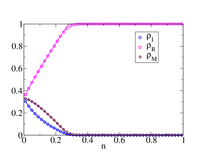
Figure 4: (color online) Stationary value of the fraction of irregulars $\rho_{I}$, regulars $\rho_{R}$ and mixed $\rho_{M}$, as a function of $n$, for the rules of model CT. Results of numerical simulations (symbols) are compared with the analytical predictions (solid lines). The rounding of the transition in simulation results is due to finite size effects.

Inserting this expression into the first equation, one is left with a third order algebraic equation, which always admits three real solutions. One of them is, for any $n$, the fully regular solution $(x,y)=(1,1)$. The two others are always unphysical (being larger than 1 or smaller than -1) except for $n\leq n_{c}=(\sqrt{17}-3)/4\approx 0.2807$. In such a case another physical solution appears

$$y=2\sqrt{-Q}\cos\left(\frac{\theta+4\pi}{3}\right),$$ (15)

where $Q=[2(n+1)-(2n+1)(2n+3)]/3$, $R=-n(2n+3)$ and $\theta=\cos^{-1}[R/\sqrt{-Q^{3}}]$. The expressions for $\rho_{R}$ and $\rho_{I}$ are obtained from the relations $\rho_{R}=(x+y)/2$ and $\rho_{I}=(x-y)/2$. The physical stationary solutions are reported in Fig. 4, along with the results of the numerical simulations of the agent-based model that well fit the theoretical predictions. The plot illustrates that the transition occurring at at $n_{c}=(\sqrt{17}-3)/4$ is continuous.

III.3 Model NT: A three-state model without a transition

Let us now focus on another set of rules, reported in Table 2, column NT. Consider the case in which an individual in the mixed state M is undecided about which one of R and I is acceptable, and let the interactions between speaker and hearer be symmetric. When an individual in a state I interacts with one in a state R both become confused on which form is right and therefore both switch to M. When an individual in a state M interacts with one in a state I or R, the outcome of the interaction depends on which form the individual in the mixed state uses: if it is the same one used by his partner (with probability 1/2) then nothing changes, if it is the alternative one (with probability 1/2) then the partner becomes confused and also switches to the mixed state M. Interactions among individuals both in the same state I or R do not produce any change. The outcome of an interaction among two individuals in a state M depends on which form they use: if they both use the regular inflection (with probability 1/4) they both switch to status R, if they both use the irregular inflection (probability 1/4) they both switch to status I, if they use different inflections (probability 1/2) they both remain in the mixed state M, coherently with the rules regulating the outcomes of the previous interactions.

It is easily seen that under this rule set the system converges to the fully regular state for any value of the ratio $r/\nu$. The MF equations are:

$$\left\{\begin{array}[]{lll}\dot{\rho}_{I}&=&-r\rho_{I}+\nu\left\{-2\rho_{I}\rho_{R}+\frac{1}{2}[1-(\rho_{I}+\rho_{R})]^{2}\right\}\\ \dot{\rho}_{R}&=&r(1-\rho_{R})+\nu\left\{-2\rho_{I}\rho_{R}+\frac{1}{2}[1-(\rho_{I}+\rho_{R})]^{2}\right\}.\end{array}\right.$$ (16)

Summing and subtracting the first equation from the second, one obtains

$$\left\{\begin{array}[]{l}\dot{y}/\nu=n(1-y)\\ \dot{x}/\nu=n(1-x)-2x+y^{2}+1\end{array}\right.$$ (17)

which shows that, for $n>0$ the fully regular state $\rho_{R}=1$, $\rho_{I}=0$ is the only possible stationary state. The conclusion is that, for any value of $\nu$ (and $n>0$), this set of rules always leads to a completely regular state for all individuals.

Unlike the previous models this one is discontinuous in the limit $n\rightarrow 0$: the model with replacement does not converge in the limit of vanishing replacement to the model with $n=0$. It is easy to see that in the case $n=0$ from Eq. (17) $\dot{y}\equiv 0$; therefore the unbalance $y_{0}$ between $\rho_{I}$ and $\rho_{R}$ present in the initial condition is preserved during the dynamics, while $x$ converges to $(1+y_{0})/2$. Therefore the stationary state is continuously dependent on the initial condition, and given by $\rho_{R}=(1+y_{0})^{2}/4$, $\rho_{I}=(1-y_{0})^{2}/4$, which gives the fully regular solution only as long as the system is initiated in the fully regular state.

To conclude this section, we observe that in three–state models different microscopic interaction rules give rise to qualitatively different behaviors. In the next section we present a general approach to the modeling schemes presented so far, clarifying why they give rise to different phenomenologies.

IV General theory

In this section we present a very general three–state model that provides a unified framework for generic sets of interaction rules, and we solve it analytically within the mean-field approximation. This framework allows us to comprehend the origin of the different behaviors found in the specific models investigated in the previous sections, providing a complete understanding of the global phenomenology of three-state models. We start by considering a general two–state model first, as this elucidates why the more complex three–state model is needed and how it behaves. We then consider a very general three-state model, encompassing all models considered before as particular cases. This approach will clarify a number of general points. In particular it will show how the nature of the transition for both two and three–state models depends on the microscopic rules, and clarify the role of asymmetries in the behavior of the speaker and hearer in the communication process.

IV.1 General two–state model

Each individual is either in state R or I. At rate $r$ each individual is replaced by one in state R. At rate $\nu$ an interaction occurs among two randomly selected individuals, the speaker and the hearer. We indicate the state of the pair of individuals in interaction as (X,Y), where X is the state of the speaker and Y of the hearer. As reasonable, we assume that nothing happens if the two individuals are in the same state [(R,R) $\rightarrow$ (R,R), (I,I) $\rightarrow$ (I,I)]. We first consider the case of deterministic rules, i.e., the state at the end of the interaction is fully determined by the initial state. Starting with the state (R,I) we parametrize the interaction rule by means of the coefficient $\gamma_{RI}$, which gives the variation in the number of individuals in state I. For example, for the interaction [(R,I) $\rightarrow$ (R,R)] $\gamma_{RI}=-1$, while for [(R,I) $\rightarrow$ (I,I)] $\gamma_{RI}=1$. Analogously, when the initial state is (I,R) the rule is parametrized by $\gamma_{IR}$.

The mean field equation for this process is simply

$$\dot{\rho}_{I}=-r\rho_{I}+\nu(\gamma_{RI}+\gamma_{IR})\rho_{I}(1-\rho_{I}).$$ (18)

Obviously $\rho_{R}=1-\rho_{I}$. It follows immediately from Eq. (18) that assuming distinct asymmetric roles between speaker and hearer has no effect whatsoever on the collective behavior, since only the cumulative coefficient $\gamma=\gamma_{RI}+\gamma_{IR}$ enters the equation. The distinction between hearer and speaker is therefore irrelevant and any model defined by an asymmetric set of rules behaves exactly as its symmetrized version. This observation allows to specify any two-state model by means of just one parameter, $\gamma$, with values between -2 and 2.

The general solution of Eq. (18) is obtained by replacing $n$ with $2n/\gamma$ in Eqs. (2) and (3). The sign of $\gamma$ determines the nature of the transition: for $\gamma>0$ (rules biased in favor of I) there exists a continuous transition with $n_{c}=\gamma$, while for $\gamma\leq 0$ (rules unbiased or biased against I) there is no transition, and the fully regular state is the only stationary solution. Therefore we conclude in general that the system is driven towards a fully regular state unless a bias in the interactions compensates for the increase in the R population due to replacement.

In the most general case, the outcome of each interaction is decided probabilistically. In this case $\gamma_{IR}$ and $\gamma_{RI}$ are defined as the average increase in I states in the interaction, each of them assuming any real value in $\left[-1,1\right]$. Correspondingly $\gamma$ can assume any real value in $[-2,2]$. It is immediate to realize that the dynamics is again described by Eq. (18) and all the above conclusions hold.

IV.2 General three–state model

As demonstrated explicitly in the case of two–state models, asymmetric interaction rules (such as those in Table 2) produce exactly the same behavior as their symmetrized version also in three–state models. It is therefore possible to express all possible interaction rules among individuals in a way analogous of what we have done for the two–state case. Let us define $\gamma_{i}$, $\phi_{i}$, and $\delta_{i}$ as the average variation in the number of individuals in state I, R or M respectively, occurring when an interaction of type $i$ takes place. We will denote with $i=1$ the interactions with initial state (I,R) and (R,I), $i=2$ for (R,M) and (M,R) , $i=3$ for (I,M) and (M,I) , $i=4$ for (M,M). As above, we are assuming that no change occurs when two individuals in state R (or two individual in state I) interact. The interaction is instead nontrivial in the case (M,M). Conservation of the number of individuals implies $\gamma_{i}+\phi_{i}+\delta_{i}=0$, for any $i=1,2,3,4$, which reduces the number of independent parameters from 12 to 8. Notice that these quantities may be non–integer when we allow for different possible final states from a given initial state (each with a given probability).

With this parametrization of the dynamical rules we can write the rate equations for the evolution of the system in the most general case:

$$\left\{\begin{array}[]{lll}\dot{\rho}_{I}/\nu&=&-n\rho_{I}+\left\{2\gamma_{1}\rho_{I}\rho_{R}+2\gamma_{2}\rho_{R}[1-(\rho_{I}+\rho_{R})]+2\gamma_{3}\rho_{I}[1-(\rho_{I}+\rho_{R})]+\gamma_{4}[1-(\rho_{I}+\rho_{R})]^{2}\right\}\\ \dot{\rho}_{R}/\nu&=&n(1-\rho_{R})+\left\{2\phi_{1}\rho_{I}\rho_{R}+2\phi_{2}\rho_{R}[1-(\rho_{I}+\rho_{R})]+2\phi_{3}\rho_{I}[1-(\rho_{I}+\rho_{R})]+\phi_{4}[1-(\rho_{I}+\rho_{R})]^{2}\right\}\end{array}\right.$$ (19)

where $n=r/\nu$ is the rate of the replacement process relative to the frequency of interaction.

We now focus on the case of unbiased interactions that do not favor either the regular or the irregular form of the verb. In other words the interaction rules are perfectly symmetric under the exchange between R and I; the only mechanism that breaks the symmetry between the regular and the irregular form is replacement, which favors the diffusion of the former. This choice is based on the observation that, while in the two-state case unbiased interaction rules always drive the system towards the fully regular state, the existence of a mixed state allows the survival of the irregular form even for some R–I symmetric interactions. This can be deduced from the three models presented in the previous section, which all have unbiased rules yet exhibit three qualitatively different behaviors. Hence symmetric interaction rules are general enough to lead to continuous or discontinuous transitions or to the absence of any transition.

The assumption of unbiased interaction implies the following additional relations among the parameters:

$$\phi_{1}=\gamma_{1}~{},~{}~{}~{}~{}\phi_{2}=\gamma_{3}~{},~{}~{}~{}~{}\phi_{3}=\gamma_{2}~{},~{}~{}~{}~{}\phi_{4}=\gamma_{4}\,,$$ (20)

thus reducing the number of free parameters to 4 (we choose to use the four $\gamma_{i}$). The values of these parameters are not arbitrary. An (R,I) interaction cannot produce an increase in the number of individuals in the I state, since the same change must occur also for individuals in the R state, since $\gamma_{1}=\phi_{1}$: hence $\gamma_{1}\leq 0$. In the same interaction the number of irregulars cannot decrease by more than 1: $-1\leq\gamma_{1}$. With similar considerations it is not difficult to verify that the $\gamma_{i}$ parameters are bounded as follows:

$$\!\!\!-1\leq\!\gamma_{1}\!\leq 0,\,\,\,0\leq\!\gamma_{2}\!\leq 2,\,\,\,-1\leq\!\gamma_{3}\!\leq 1,\,\,\,0\leq\!\gamma_{4}\!\leq 1.$$ (21)

Introducing the relations (20) in Eqs. (19) it is possible to write Eqs. (19) in a particularly simple form by defining the auxiliary quantities $x=\rho_{R}+\rho_{I}$ and $y=\rho_{R}-\rho_{I}$, which represent the fraction of individuals in an unmixed state, and the excess fraction of R states with respect to I states, respectively:

$$\left\{\begin{array}[]{l}\dot{x}/\nu=ax^{2}+cy^{2}+2dx+f\\ \dot{y}/\nu=(2(\gamma_{3}-\gamma_{2})-n)y-2(\gamma_{3}-\gamma_{2})xy+n\end{array}\right.$$ (22)

where

$$\begin{array}[]{llllllll}a&=&\gamma_{1}-2(\gamma_{2}+\gamma_{3})+2\gamma_{4}&&&c&=&-\gamma_{1}\\ d&=&(\gamma_{2}+\gamma_{3})-2\gamma_{4}-n/2&&&f&=&2\gamma_{4}+n.\end{array}$$ (23)

Physically sensible solutions must be in the range $0\leq x\leq 1$ and $-x\leq y\leq x$. Notice that $c\geq 0$, $f\geq 0$, while the sign of $a$ and $d$ may vary and the coefficients are related by

$$a+c+2d+f=0\,.$$ (24)

Equation (24) implies that, for any choice of the parameters, $(x,y)=(1,1)$ [which corresponds to the fully regular state ($\rho_{R}=1,\rho_{I}=0$)] is always a stationary solution of Eq. (22). By imposing stationarity in Eqs. (22), other stationary solutions can be determined. For specific values of the parameters $\gamma_{i}$ it is always straightforward to solve analytically for the stationary solutions of Eqs. (22) (which boils down to the solution of a third-order algebraic equation) and study their behavior as a function of $n$.

In the following we derive instead in full generality conditions on the parameters $\gamma_{i}$ for the existence, as a function of $n$, of a continuous transition, a discontinuous one or no transition at all.

IV.2.1 Case $\gamma_{3}=\gamma_{2}$: No-transition

Let us first consider the special class of models with $\gamma_{3}=\gamma_{2}$. In this case the second of Eqs. (22) trivially yields at stationarity $y=1$, giving the two solutions $(x_{1},y_{1})=(1,1)$ and $(x_{2},y_{2})=(-(2d+a)/a,1)$. The second solution is always unphysical. Indeed, from Eq. (24) it follows that $-(2d+a)>0$. Hence $x_{2}$ is smaller than 0 if $a<0$. On the other hand, for $\gamma_{3}=\gamma_{2}$ the value of $\gamma_{3}+\gamma_{2}$ is always positive, since $\gamma_{2}\geq 0$. This implies $-(2d+a)>a$ so that $x_{2}>1$ if $a>0$. We conclude that when $\gamma_{3}=\gamma_{2}$ the only possible stationary state is the fully regular one: no transition may occur. As shown in Table 3 the NT model considered in the previous section falls in this class of models, featuring $\gamma_{2}=\gamma_{3}=0$. We will see below that also the degenerate case $\gamma_{1}=0$ implies no transition, irrespective of the value of the other parameters.

	Model NT	Model CT	Model NG
$\,\,\,\,\gamma_{1}\,\,\,\,\,\,\,\,$	-1	-1/2,	-1/2
$\,\,\,\,\gamma_{2}\,\,\,\,\,\,\,\,$	0	1/4	0
$\,\,\,\,\gamma_{3}\,\,\,\,\,\,\,\,$	0	0	1/2
$\,\,\,\,\gamma_{4}\,\,\,\,\,\,\,\,$	1/2	1/2	1

Table 3: The table summarizes the values of the set of $\gamma_{i}$ parameters for the three models studied in the previous section.

IV.2.2 Case $\gamma_{3}\neq\gamma_{2}$: Existence of a transition

Assuming now $\gamma_{3}\neq\gamma_{2}$, and imposing stationarity in Eq. (22), we get

$$\left\{\begin{array}[]{lr}ax^{2}+cy^{2}+2dx+f=0&\,\,\,\,\,\,\left[{\cal C}_{1}\right]\\ y\left(x-(1-\epsilon)\right)=\epsilon&\,\,\,\,\,\,\left[{\cal C}_{2}\right]\end{array}\right.$$ (25)

where $\epsilon=n/[2(\gamma_{3}-\gamma_{2})]$. The solutions of Eq. (25) are given by the intersections between two conic sections ${\cal C}_{1}$ and ${\cal C}_{2}$. ${\cal C}_{2}$ is an hyperbola with asymptotes $y=0$, and $x=1-\epsilon$. Depending on the sign of $\epsilon$, the two branches of the hyperbola lie in different quadrants with respect to the asymptotes (see Fig. 5).

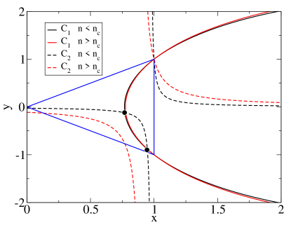
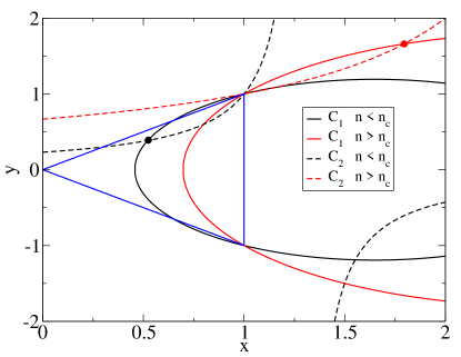
Figure 5: (color online) Plot of the two conic sections ${\cal C}_{1}$ and ${\cal C}_{2}$ for $\gamma_{3}>\gamma_{2}$ (top) and for $\gamma_{3}<\gamma_{2}$ (bottom), illustrating the intersections above [red (gray) curves] and below (black curves) the critical $n_{c}$. The triangle is the region of physical interest. The circles denote the intersections other than the fully regular solution.

In the limit $\epsilon\rightarrow 0$, which corresponds to the case with no replacement, the hyperbola degenerates into the pair of asymptotes, $y=0$ and $x=1$. The conic section ${\cal C}_{1}$ is an ellipse for $a>0$ and an hyperbola for $a<0$, turning into a parabola for $a=0$, with axes in all cases parallel to the Cartesian coordinate system. The intersections of ${\cal C}_{1}$ with the $y=0$ axis are, for $a\neq 0$,

$$x_{1}=\frac{-d-\Delta}{a}\,,~{}~{}~{}~{}~{}x_{2}=\frac{-d+\Delta}{a}\,,$$ (26)

where $\Delta=\sqrt{d^{2}-af}=\sqrt{(d+f)^{2}+cf}>0$. It is not difficult to show that $x_{1}$ is always physical (between 0 and 1) while $x_{2}$ is always unphysical (see Appendix B). In particular, $x_{2}>1$ if $a>0$ and $x_{2}<0$ if $a<0$. In the limit $a\rightarrow 0$, $x_{1}\rightarrow-f/(2d)$ (which is the intersection point for the parabolic case $a=0$) while $x_{2}\rightarrow\pm\infty$, depending on the sign of $a$. Hence, despite the change in the global behavior for different values of $a$, ${\cal C}_{1}$ has always a similar shape in the region of physical interest $0\leq x\leq 1$: it crosses the $y=0$ axis for $x=x_{1}$ and is concave towards the right, passing through the two points $(x,y)=(1,1)$ and $(x,y)=(1,-1)$ for any value of the parameters. Notice that also ${\cal C}_{2}$ always goes through the point $(x,y)=(1,1)$, so that the fully regular state is always a stationary solution.

We now investigate in full generality the possible existence of other stationary solutions, i.e. other intersections in the physical region. Only the case $c=0$ ($\gamma_{1}=0$) needs to be treated separately, because the conic section ${\cal C}_{1}$ degenerates into a pair of lines: $(x-1)(x+(2d+a)/a)=0$, one ($x=1$) on the boundary of the physical region, the other outside it. The fully regular solution $(x,y)=(1,1)$ is then the only stationary state, and there is no transition. We will assume $c\neq 0$ in what follows.

$\gamma_{3}>\gamma_{2}$: Discontinuous transition.

For $\gamma_{3}>\gamma_{2}$ ($\epsilon>0$), the hyperbola ${\cal C}_{2}$ lies in the upper–right and lower–left quadrants with respect to the asymptotes (see Fig. 5). Notice that the vertical asymptote is always at $x<1$. Apart from the fully regular solution, one intersection occurs always for $x<0$ or $x>1$ and is thus unphysical. Two other intersections may instead occur between ${\cal C}_{1}$ and the lower–left branch of ${\cal C}_{2}$. For large $n$ these intersections do not exist as it can be recognized by observing that for $\epsilon>1$ the lower branch of ${\cal C}_{2}$ has $x<0$ while ${\cal C}_{1}$ has $x>x_{1}>0$. However, when $n\to 0$, ${\cal C}_{2}$ shrinks towards its asymptotes $x=1-\epsilon$ and $y=0$, while ${\cal C}_{1}$ does not change much. At some critical value $n=n_{c}$, ${\cal C}_{2}$ starts intersecting ${\cal C}_{1}$, so that for $n<n_{c}$ there are two intersections (see Fig. 5), both in the physical region because the derivative of ${\cal C}_{1}$ for $x=1$ is $-[1+(d+f)/c]<-1$. In this case the system undergoes a discontinuous transition at $n_{c}$. Notice when these two solutions exist they are in the region $y\leq 0$, implying that $\rho_{I}\geq\rho_{R}$, i.e., the fraction of individuals in the I state is larger than the fraction of those in the R state. As indicated in Table 3, the model NG, which features $\gamma_{3}-\gamma_{2}=1/2$, belong to this class and this explains why it undergoes a discontinuous transition.

$\gamma_{3}<\gamma_{2}$: Continuous transition.

For $\gamma_{3}<\gamma_{2}$ ($\epsilon<0$), the hyperbola ${\cal C}_{2}$ lies in the upper–left and lower–right quadrants (see Fig. 5). The lower branch has $x>1-\epsilon>1$ and hence is unphysical. Therefore at most two of the four solutions (the intersections of the upper branch with ${\cal C}_{1}$) are physical. One of them is the fully regular state. To investigate the location of the other intersection one can compare the slope of the two conic sections for $x=1$. If the slope of ${\cal C}_{1}$ is larger than the slope of ${\cal C}_{2}$ (which happens for large $n$) the second intersection occurs for $x>1$, it is unphysical and as a consequence the fully regular state is the only stationary solution. If $n$ is reduced the slope of ${\cal C}_{1}$ at $x=1$ decreases while the slope of ${\cal C}_{2}$ grows. At a critical value $n_{c}$ the two slopes are equal and for $n<n_{c}$ the second intersection becomes physical ($x<1$). We conclude therefore that the system undergoes a continuous transition between a fully regular state and a state with coexisting regular and irregular individuals. Notice that in this case, since the physical intersections have $y\geq 0$, necessarily $\rho_{I}\leq\rho_{R}$. The value of $n_{c}$ is easily determined by the condition that the two slopes are equal, and turns out to be

$$n_{c}=(\gamma_{1}\!-\!\gamma_{2}\!-\!\gamma_{3})\!\pm\!\sqrt{(\gamma_{1}\!-\!\gamma_{2}\!-\!\gamma_{3})^{2}+4\gamma_{1}(\gamma_{3}-\gamma_{2})}$$ (27)

which has always one positive value (the other being always negative), coherently with the fact that there is always a transition. Remarkably, the value of $n_{c}$ does not depend at all on the coefficient $\gamma_{4}$, regulating the M-M interaction. The model CT in the previous section has $\gamma_{3}=0$, $\gamma_{2}=1/4$ and $\gamma_{1}=-1/2$ (see Table 3). These values explain why it undergoes a continuous transition at $n_{c}=(\sqrt{17}-3)/4$.

IV.2.3 Stability analysis

So far we have shown that below some critical value of $n$ additional stationary solutions appear, beyond the fully regular solution. To complete the demonstration of the existence of phase-transitions we must analyze their stability.

By linearizing Eqns. (22) around the solution $(x^{*},y^{*})$ one gets:

$$\!\frac{1}{2\nu}\frac{d}{dt}\!\left[\begin{array}[]{cc}\delta x\\ \delta y\end{array}\right]\!=\!\left[\begin{array}[]{cc }ax^{*}+d&cy^{*}\\ -(\gamma_{3}-\gamma_{2})y^{*}&(\gamma_{3}-\gamma_{2})(1-x^{*})-\frac{n}{2}\end{array}\right]\!\left[\begin{array}[]{cc}\delta x\\ \delta y\end{array}\right].$$ (28)

For the fully regular state $(x^{*},y^{*})=(1,1)$ the eigenvalues of the stability matrix $M$ can be evaluated explicitly yielding

$$\lambda_{1,2}=[\operatorname{tr}(M)\pm\sqrt{\Delta_{1}}]/2$$ (29)

where the trace of the matrix is $\operatorname{tr}(M)=\gamma_{1}-\gamma_{2}-\gamma_{3}-n$ and $\Delta_{1}=(\gamma_{1}+\gamma_{2}+\gamma_{3})^{2}-8\gamma_{1}\gamma_{2}\geq 0$. Notice that $\Delta_{1}$ is independent of $n$ and positive, implying that the two eigenvalues are always real.

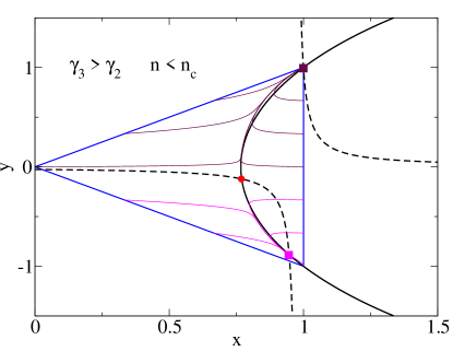
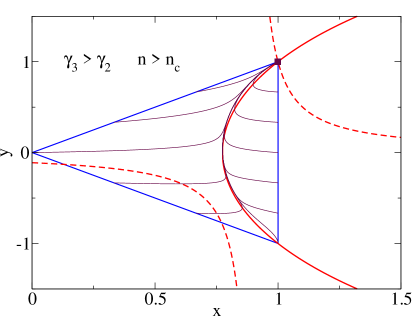
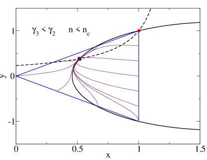
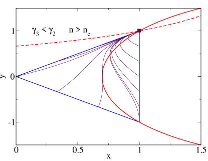
Figure 6: (color online) Phase-flow in the $(x,y)$ space for discontinuous (top) and continuous (bottom) transition both below (left) and above (right) the transition. The triangle is the region of physical interest. The thick curves are ${\cal C}_{1}$ (solid) and ${\cal C}_{2}$ (dashed). Symbols indicate stationary solutions. The red circles are saddle points with an attractive and a repulsive direction. The squares are attractive stable solutions. Thin solid lines are flow lines converging to the stable solution denoted by symbols with the same color (shade).

In the case $\gamma_{3}>\gamma_{2}$, both eigenvalues are negative, as can be deduced by considering that $\operatorname{tr}(M)$ (the sum of the eigenvalues) is always negative (being the sum of four negative terms) and $\det(M)=n^{2}/4-n(\gamma_{1}-\gamma_{2}-\gamma_{3})/2-\gamma_{1}(\gamma_{3}-\gamma_{2})$ (the product of the eigenvalues) is always positive for $n>0$. This last condition can be understood by considering that $\det(M)$ is a parabola with upward concavity and zeros for negative values of $n$ [given by Eq. (27)]. Hence, the fully regular state is always stable. For small $n$, the two other solutions appearing in the physical region are a saddle and a stable fixed point [see Fig. (6)]: a discontinuous transition occurs.

In the case $\gamma_{3}<\gamma_{2}$, corresponding to a continuous transition, $\det(M)$ is positive for large $n$, but it changes sign for $n<n_{c}$ [where $n_{c}$ is the only positive determination of Eq. (27)] thus implying that one of the eigenvalues becomes positive. Hence, below the transition the fully regular state corresponds to a saddle, while the other solution appearing in the physical region is stable [see Fig. (6)].

Finally, we remark that the parameters corresponding to the Naming Game, considered in the previous section as an example of models with discontinuous transition, give $\Delta_{1}=0$, corresponding to two degenerate eigenvalues, and only one eigenvector. In this case the fully regular state is stable but defective: in principle arbitrarily small changes of the parameters may result in a standard stable fixed point if $\Delta_{1}>0$, or in a stable spiral when $\Delta_{1}<0$. This last case would change the physical picture, because spiralling trajectories would cross the boundary of the physical domain before reaching the fixed point, and therefore the physical system would be driven toward the boundary of the physical region without reaching the fixed point. However, this possibility is ruled out by the condition $\Delta_{1}\geq 0$ which holds for physically sensible values of the parameters $\gamma_{i}$.

IV.2.4 Wrap-up of the theory for the general model

The conclusions that follow from the theory presented in this section are very general and simple. The existence and the nature of a transition depends only on the sign of $\gamma_{3}-\gamma_{2}$. If $\gamma_{3}>\gamma_{2}$, as the frequency increases a discontinuous transition occurs between a fully regular state and a state with coexistence of fully regular and mostly irregular inflections. If $\gamma_{3}<\gamma_{2}$, the transition is instead continuous. If $\gamma_{3}=\gamma_{2}$, no transition occurs and the system always reaches a fully regular state.

It is important to notice that the condition $\gamma_{3}>\gamma_{2}$ has a very natural interpretation in the context of language dynamics. It simply means that (recalling that $\gamma_{2}=\phi_{3}$) an interaction between an individual in state M and one in state I, will produce an increment in the use of the irregular inflection larger than the increment in the use of the regular inflection. The fact that this asymmetry alone is sufficient to give rise to a discontinuous transition is a strong indication of the relevance of these theoretical modeling efforts for the interpretation of empirical data.

V Conclusions

This work has presented an investigation of agent-based models aimed at understanding the processes regulating the interplay between rules and exceptions in language dynamics. In particular, the models aim to investigate the observed behavior of verbs in natural language. Corpus data from natural language points to the existence of a discontinuous transition as a function of the frequency of usage: high frequency items are highly irregular and low frequency ones are regular, while in an intermediate frequency range coexistence between the two behaviors is observed.

In the minimal models considered each agent is endowed with an inventory, containing the possible inflections (regular or irregular) of a lemma. Two processes have the potential to change agents’ inventories over time: interaction and replacement. In interaction, individuals influence each other, adding or deleting forms from their inventories according to a specific set of interaction rules. In replacement events, agents are substituted by new “child” individuals, who are automatically biased towards the regular form by being “born” with a regular inventory.

We analyze two classes of models. In the first one each individual may store in the inventory only one of the two competing inflections, either the regular or the irregular one. Three-state models instead integrate a mixed state, which represents an individual who finds both the regular and irregular forms acceptable. We solve these models analytically within the mean-field framework and confirm the results by means of numerical simulations. We first focus on a few specific models, including the Naming Game for language dynamics. The analysis reveals that the the global phenomenology changes qualitatively depending on the interaction rules: one can observe the absence of a transition with a move to total regularity, a continuous transition, or a discontinuous one. We then consider a very general three-state model, encompassing all previous examples as special cases, which allows the description of the previous models with a set of four minimal parameters describing the interaction rules. From this comprehensive approach several results follow:
(i) Asymmetries in the influence of the speaker and of the hearer in interaction do not play any role in the collective behavior of the system.
(ii) In two-state models the fully regular state is the only attractor unless the interaction rules are biased in favour of the irregular inflection; the three-state models have instead nontrivial behavior even when the rules are unbiased.
(iii) Allowing for a third state is crucial for the appearance of a discontinuous transition that cannot arise in two–state versions of the model.
(iv) In three state models the quantity $\gamma_{3}-\gamma_{2}$ rules the macroscopic behavior by changing the nature of the transition: when $\gamma_{3}>\gamma_{2}$, a discontinuous transition is observed to a state where irregular inflection is prevalent ($\rho_{I}>\rho_{R}$); in the opposite case, when $\gamma_{3}>\gamma_{2}$ a continuous transition is observed, to a state with $0<\rho_{R}<\rho_{I}$; in the case $\gamma_{3}=\gamma_{2}$ there is no transition and the fully regular state is reached for any frequency.
(v) In the case $\gamma_{3}>\gamma_{2}$, above the discontinuous transition the steady state depends on the initial condition: verbs with the same frequency can end up as fully regular or mostly irregular, similarly to what is observed in empirical data.
(vi) In the context of language dynamics, the condition $\gamma_{3}>\gamma_{2}$ is satisfied by sets of more plausible rules, so that a discontinuous transition is to be expected.

This model provides a framework that could potentially be used to consider additional, more complex aspects of rule dynamics in language. In particular, empirical data shows that the growth of language contributes to the expansion of regularity Cuskley et al. (2014a), since a core aspect of a linguistic rule’s utility is that it can be generatively applied to new forms (e.g., the past tense of the neologism selfie is uncontroversially selfied). Our model considers a word’s frequency to be static over time; however, natural languages are living, and populations, vocabulary sizes, and turnover rates are not static. Furthermore, there are other cognitive mechanisms beyond child learner biases that may contribute to regularity dynamics. General memory constraints may contribute to the persistence of highly frequent irregular forms Cuskley et al. (2014b), and adult learners may possess qualitatively different regularization biases from children Hudson Kam and Newport (2009). Moreover, the use of a disordered topology for the pattern of interaction, as opposed to the homogeneous mixing assumed by the MF approach, combined with the interaction among the different lemmas in the agents’ inventories may lead to different patterns of regularization in frequency. Future models might also consider another key aspect in the persistence of irregularity: the notion that irregular forms are not always exceptions, but sometimes constitute sub-rules Yang (2005) (e.g., foot-feet/goose-geese, sing-sang/ring-rang). Our model provides a basic starting point from which to consider the complex dynamics underlying temporal trends of the rules that form the core of language.

Finally, it is very important to stress that while models and results are presented in this paper in terms of linguistic rule dynamics, they are fully general and apply to any system where individuals have three possible internal states and the population exhibits turnover. The results presented in this paper, and in particular the conditions determining the existence of a transition and its nature, may have strong implications not only for linguistic rules, but also for all those systems.

VI Appendix

VI.1

In this appendix we report the stability analysis for the Naming Game without biased replacement, i.e., with $n=0$ as discussed in Sec. III.1. For the case $n=0$ the stability matrix is given by:

$$\frac{d}{dt}\left[\begin{array}[]{cc}\delta\rho_{I}\\ \delta\rho_{R}\end{array}\right]=\left[\begin{array}[]{cc }-1&2(\rho_{R}-1)\\ 2(\rho_{I}-1)&-1\end{array}\right]\left[\begin{array}[]{cc}\delta\rho_{I}\\ \delta\rho_{R}\end{array}\right]$$ (30)

whose eigenvalues are:

$$\lambda_{1,2}=\pm\sqrt{4(\rho_{I}^{*}-1)(\rho_{R}^{*}-1)}-1,$$ (31)

where, as before, ($\rho_{I}^{*}$, $\rho_{R}^{*}$) indicates the generic stationary solution. For ($\rho_{I}^{(1)}$, $\rho_{R}^{(1)}$) and ($\rho_{I}^{(2)}$, $\rho_{R}^{(2)}$) both eigenvalues are negative and the solutions are both stable. For ($\rho_{I}^{(3)}\simeq 0.382$, $\rho_{R}^{(3)}\simeq 0.382$) the eigenvalues are one positive ($\lambda_{1}=2.236$) and one negative ($\lambda_{2}=-4.236$) and this corresponds to a saddle point with an attractive and a repulsive direction. The separatrix in Fig. 3 (left) in the attractive direction corresponds to the eigenvector associated to the negative eigenvalue: $\rho_{R}=\rho_{I}$ (the red line in figure). The other separatrix is locally approximated (in the neighborhood of ($\rho_{I}^{(3)}$, $\rho_{R}^{(3)}$), by the eigenvector associated to the positive eigenvalue $\rho_{R}=-\rho_{I}+2\rho_{I}^{(3)}$ (the green line in figure). The phase flow is such that if the initial condition is such that $\rho_{I}<\rho_{R}$ ($\rho_{I}>\rho_{R}$) the system will deterministically converge to the regular (irregular) state. On the other hand if the initial condition is such that $\rho_{I}=\rho_{R}$ the system will converge to the stationary solution ($\rho_{I}^{(3)}$, $\rho_{R}^{(3)}$) (see also Refs. Baronchelli et al. (2007, 2008)).

VI.2

In this appendix, we provide explicit proofs that the intersections $x_{1}$ and $x_{2}$ of the conic section $\cal{C}_{1}$ with the axis $y=0$ [see Eq. (26)] are always physical and always unphysical, respectively.

Let us first consider the case $a>0$. A crucial point to recognize is that, since $a+2d=-(c+f)<0$, if $a$ is positive $d$ must be negative. Hence $\Delta=\sqrt{d^{2}-af}\leq|d|=-d$. As a consequence $x_{1}=-(\Delta+d)/a\geq 0$. The alternative expression of $\Delta=\sqrt{(a+d)^{2}+ac}$ implies, since both $a$ and $c$ are positive, $\Delta\geq|a+d|$. This means that $\Delta\geq-(a+d)$ so that $x_{1}=-(\Delta+d)/a\leq 1$. It also implies $\Delta\geq(a+d)$ which, inserted into the expression $x_{2}=(\Delta-d)/a\geq 1$, yields $x_{2}\geq 1$.

The arguments are similar for $a<0$. In this case $\Delta=\sqrt{d^{2}-af}\geq|d|\geq-d$ so that $x_{1}=(-d-\Delta)/a\geq 0$. By the same token $\Delta=\sqrt{d^{2}-af}\geq d$, implying $x_{2}=(\Delta-d)/a\leq 0$. Finally, to show that $x_{1}\leq 1$ we start from $\Delta=\sqrt{(a+d)^{2}+ac}\leq|a+d|$. The quantity $a+d$ is negative for $a<0$, because $a+2d<0$ implies $2a+2d<a<0$. Hence $\Delta\leq|a+d|=-(a+d)$ so that $x_{1}=-(d+\Delta)/a<1$.

References

- Hockett (1961) C. F. Hockett, Language 37, 29 (1961).
- Chomsky (1986) N. Chomsky, Knowledge of language: Its nature, origin, and use (Greenwood Publishing Group, Santa Barbara, CA, 1986).
- Pinker (1999) S. Pinker, Words and rules: The ingredients of language. (Basic Books, New York, 1999).
- McClelland and Patterson (2002) J. L. McClelland and K. Patterson, Trends in Cognitive Sciences 6, 464 (2002).
- Pinker and Ullman (2002) S. Pinker and M. T. Ullman, Trends in cognitive sciences 6, 456 (2002).
- Bybee and Slobin (1982a) J. L. Bybee and D. I. Slobin, Language 58, 265 (1982a).
- Marslen-Wilson and Tyler (1998) W. Marslen-Wilson and L. K. Tyler, Trends in cognitive sciences 2, 428 (1998).
- Plunkett and Marchman (1996) K. Plunkett and V. A. Marchman, Cognition 61, 299 (1996).
- Cuskley et al. (2014a) C. F. Cuskley, M. Pugliese, C. Castellano, F. Colaiori, V. Loreto, and F. Tria, PLoS ONE 9, e102882 (2014a).
- Lieberman et al. (2007) E. Lieberman, J.-B. Michel, J. Jackson, T. Tang, and M. A. Nowak, Nature 449, 713 (2007).
- Carroll et al. (2012) R. Carroll, R. Svare, and J. C. Salmons, Journal of Historical Linguistics 2, 153 (2012).
- Baronchelli et al. (2008) A. Baronchelli, V. Loreto, and L. Steels, International Journal of Modern Physics C 19, 785 (2008).
- Loreto et al. (2011) V. Loreto, A. Baronchelli, A. Mukherjee, A. Puglisi, and F. Tria, Journal of Statistical Mechanics: Theory and Experiment 2011, P04006 (2011).
- Labov (1972) W. Labov, Sociolinguistic patterns, 4 (University of Pennsylvania Press, Philadelphia, 1972).
- Dale and Lupyan (2012) R. Dale and G. Lupyan, Advances in complex systems 15, 1150017 (2012).
- Berman (1981) R. A. Berman, Stanford Papers and Reports on Child Language Development 20, 34 (1981).
- Bybee and Slobin (1982b) J. L. Bybee and D. I. Slobin, in Papers from the 5th international conference on historical linguistics, Vol. 21 (John Benjamins Publishing Company, Amsterdam, 1982).
- Maslen et al. (2004) R. J. Maslen, A. L. Theakston, E. V. Lieven, and M. Tomasello, Journal of Speech, Language, and Hearing Research 47, 1319 (2004).
- Abrams and Strogatz (2003) D. M. Abrams and S. H. Strogatz, Nature 424, 900 (2003).
- Marro and Dickman (1999) J. Marro and R. Dickman, Nonequilibrium phase transitions in lattice models (Cambridge University Press, Cambridge, 1999).
- Castellano et al. (2009) C. Castellano, S. Fortunato, and V. Loreto, Reviews of Modern Physics 81, 591 (2009).
- Wang and Minett (2005) W. S.-Y. Wang and J. W. Minett, Trends in Ecology and Evolution 20, 263 (2005).
- Minett and Wang (2008) J. W. Minett and W. S.-Y. Wang, Lingua 118, 19 (2008).
- Castelló et al. (2006) X. Castelló, V. M. Eguíluz, and M. San Miguel, New Journal of Physics 8, 308 (2006).
- Clifford and Sudbury (1973) P. Clifford and A. Sudbury, Biometrika 60, 581 (1973).
- Holley and Liggett (1975) R. Holley and T. Liggett, Annals of Probability 3, 643 (1975).
- Baronchelli et al. (2006) A. Baronchelli, M. Felici, E. Caglioti, V. Loreto, and L. Steels, Journal of Statistical Mechanics: Theory and Experiment (2006), 10.1088/1742-5468/2006/06/P06014.
- Puglisi et al. (2008) A. Puglisi, A. Baronchelli, and V. Loreto, Proc. Natl. Acad. of Sci. USA 105, 7936 (2008).
- Mukherjee et al. (2011) A. Mukherjee, F. Tria, A. Baronchelli, A. Puglisi, and V. Loreto, PLoS ONE 6, e16677 (2011).
- Tria et al. (2012) F. Tria, B. Galantucci, and V. Loreto, PLoS ONE 7, e37744 (2012).
- Baronchelli et al. (2007) A. Baronchelli, L. Dall’Asta, A. Barrat, and V. Loreto, Phys. Rev. E 76, 051102 (2007).
- Cuskley et al. (2014b) C. Cuskley, C. Castellano, F. Colaiori, V. Loreto, M. Pugliese, and F. Tria, “Frequency and stability of linguistic variants,” in The Evolution of Language (World Scientific, Singapore, 2014) Chap. 72, pp. 417–418.
- Hudson Kam and Newport (2009) C. L. Hudson Kam and E. L. Newport, Cognitive Psychology 59, 30 (2009).
- Yang (2005) C. Yang, Linguistic variation yearbook 5, 265 (2005).