Many-body processes in black and grey matter-wave solitons

Abstract

We perform a comparative beyond mean-field study of black and grey solitonic excitations in a finite ensemble of ultracold bosons confined to a one-dimensional box. An optimized density-engineering potential is developed and employed together with phase-imprinting to cleanly initialize grey solitons. Based on our recently developed Multi-Layer Multi-Configuration Time-Dependent Hartree Method for Bosons, we demonstrate that quantum fluctuations limit the lifetime of the soliton contrast, which prolongs with increasing soliton velocity. A natural orbital analysis reveals a two-stage process underlying the decay of the soliton contrast. The broken parity symmetry of grey solitons results in a local asymmetry of the orbital mainly responsible for the decay, which leads to a characteristic asymmetry of remarkably localized two-body correlations. The emergence and decay of these correlations as well as their displacement from the instantaneous soliton position are analysed in detail. Finally, the role of phase-imprinting for the many-body dynamics is illuminated and additional non-local correlations in pairs of counter-propagating grey solitons are unravelled.

I Introduction

Solitons are very peculiar solutions of non-linear wave equations emerging in various fields of physics ranging from non-linear optics to shallow water waves Remoissenet (1999); Dauxois and Peyrard (2006). These solutions are characterized by their form-stability under time evolution and even under collisions so that solitons can behave akin to classical particles and may be described as such under certain conditions. In particular, ultracold bosonic quantum gases allow both theoretically and experimentally for thorough investigations of dark solitons, i.e. localized density minima accompanied by characteristic phase jumps in the order parameter, residing on the background density profile of trapped atomic clouds (Kevrekidis et al. (2008); Frantzeskakis (2010) and ref. therein). The fully integrable Gross-Pitaevskii mean-field equation for a quasi-one-dimensional uniform, perfect Bose-Einstein condensate, for instance, posseses a dark soliton solution Tsuzuki (1971); Pethick and Smith (2008); Kevrekidis et al. (2008); Frantzeskakis (2010) completely characterized by the ratio $\beta$ of soliton velocity $u$ to the speed of sound $s=\sqrt{\rho_{0}g/m}$:

$$\psi_{\beta}(x,t)= \sqrt{\rho_{0}}e^{-i\mu_{0}t/\hbar}\;\times$$

$$\times\;\left(i\beta+\eta\tanh\Big{(}\eta\frac{x-\beta st-x_{0}}{\xi}\Big{)}\right),$$

with $|\beta|\leq 1$, $\eta=\sqrt{1-\beta^{2}}$, bulk density $\rho_{0}$, chemical potential $\mu_{0}=\rho_{0}g$, healing length $\xi=\hbar/\sqrt{m\rho_{0}g}$, atomic mass $m$ and contact interaction strength $g$. Black solitons ($\beta=0$) do not move and feature a density notch with a phase jump of $\pi$, while grey solitons ($|\beta|>0$) are moving objects with a finite density minimum and a smaller phase jump.

As excited states, however, dark solitons may suffer from various sources of instabilities ranging from thermodynamic (e.g. Muryshev et al. (2002); Gangardt and Kamenev (2010); Cockburn et al. (2011) and ref. therein) and dynamical instabilities (e.g. Muryshev et al. (2002); Brand and Reinhardt (2002); Becker et al. (2013); Ku et al. (2014); Donadello et al. (2014); Muñoz Mateo and Brand (2014) and ref. therein) to decay as a consequence of quantum fluctuations. Since nowadays experiments can be operated at effectively zero temperature and with a high aspect ratio of the transverse and longitudinal traps, ultracold bosonic quantum gases serve as ideal systems for exploring the quantum nature and correlation effects in solitonic excitations. The number of atoms and the interaction strength obviously constitute key parameters, which determine the intensity of correlations and are, most importantly, controllable in nowadays experiments. In passing, we note that also the illumination of beyond mean-field effects in vortex excitations has recently attracted interest Dagnino et al. (2009); Weiner et al. (2014); Tsatsos and Lode (2014); Wells et al. (2014).

Usually, the form-stability of the dark solitons is regarded as a compensation of dispersion by the non-linearity of the Gross-Pitaevskii equation Tsuzuki (1971). The actual many-body Schrödinger equation, however, is linear and should also be able to describe solitons in appropriate parameter regimes. The ongoing theoretical efforts from this linear perspective can be classified into two directions: The deductive approach Kulish et al. (1976); Ishikawa and Takayama (1980); Kanamoto et al. (2010); Sato et al. (2012a, b); Wadkin-Snaith and Gangardt (2012); Astrakharchik and Pitaevskii (2013); Draxler et al. (2013); Karpiuk et al. (2015) aims at establishing a relation between the hole-like type II excitations of the solvable Lieb-Liniger model Lieb and Liniger (1963); Lieb (1963) and the Gross-Pitaevskii soliton solutions Tsuzuki (1971). In contrast to this, we follow the inductive approach in which one either starts with a mean-field product state featuring a soliton or uses experimentally relevant protocols to prepare a many-body state resembling the properties of a dark soliton. The subsequent time-evolution is then studied with beyond mean-field methods.

Shortly after the first experimental implementation of dark solitons in Bose-Einstein condensates Burger et al. (1999), the inductive approach studies predicted a dynamical instability due to quantum fluctuations Dziarmaga et al. (2002); Dziarmaga and Sacha (2002); Law et al. (2002); Dziarmaga et al. (2003); Law (2003); Dziarmaga and Sacha (2006); Dziarmaga (2004); Mishmash and Carr (2009); Mishmash et al. (2009); Martin and Ruostekoski (2010); Delande and Sacha (2014): The density minimum of a dark soliton is incoherently filled with atoms on potentially experimentally relevant time scales. On the one hand side, this dynamical quantum depletion effect has been studied within the Bogoliubov perturbation theory Dziarmaga and Sacha (2002); Law et al. (2002); Dziarmaga et al. (2003); Law (2003); Dziarmaga and Sacha (2006) as well as a non-perturbative variant Dziarmaga (2004) highlighting the role of the localized zero (anomalous) mode in uniform (trapped) systems as main contributor to the filling of the density minimum. On the other hand, the numerically exact time-evolving block-decimation technique (TEBD) has been employed in finite lattices Mishmash and Carr (2009); Mishmash et al. (2009) and continuous systems within the Bose-Hubbard approximation Delande and Sacha (2014). As the main experimental signatures, the relaxation of the reduced one-body density to a flat profile and a quantum fluctuation induced inelasticity of a binary soliton collision were reported. Moreover, at times when the reduced one-body density, i.e. the average over many single shot measurements, has already relaxed to a flat distribution, the histograms of simulated destructive $N$-atom single shot measurements have revealed a soliton-like density minimum at random positions Dziarmaga et al. (2003); Dziarmaga and Sacha (2006); Dziarmaga et al. (2010); Mishmash and Carr (2010); Delande and Sacha (2014). These findings suggest the existence of highly non-trivial correlations being unravelled in single shot measurements.

The above works have almost exclusively focussed on black solitons and, except for some side aspects of Wadkin-Snaith and Gangardt (2012); Dziarmaga (2004); Mishmash and Carr (2009); Mishmash et al. (2009), grey solitons have not been studied beyond the mean-field approximation so far. Therefore, this work aims at a systematic comparison of beyond mean-field signatures in black solitons and their experimentally more relevant grey counterparts. Having introduced our setup and the employed ab initio method in Sect. II.1 and II.2, respectively, we present a semi-analytically optimized density-engineering scheme, which allows, in combination with a phase-imprinting procedure, to robustly and cleanly generate grey solitons (Sect. II.3). Although the broken parity symmetry of a grey soliton results in a larger variety of allowed incoherent scattering channels compared to a black soliton of well defined parity, grey solitons prove to be more stable in terms of a longer contrast lifetime (Sect. III.1) and slower dynamical quantum depletion (Sect. III.2). Despite of the extensive literature on many-body effects in black solitons, the evolution of local two-body correlations, which are experimentally accessible via density-density correlation measurements, has not been investigated so far. In Sect. III.3, we explore the occurrence of spatially well localized bunching and antibunching correlations for dark solitons: Whereas these correlations are symmetrically arranged around a black soliton of well defined parity, the localized bunching correlations become displaced to the back of a grey soliton with subsonic velocity while emerging. The characteristic asymmetric correlation pattern of a grey soliton is traced back to a local asymmetry of the single-particle state most responsible for the soliton decay. In Sect. III.4, the role of the phase-imprinting is illuminated, demonstrating that imposing a phase profile accelerates the quantum decay while omitting this procedure results in pairs of counter-propagating, long-living grey solitons. Besides the localized two-body correlations identified for a single grey soliton, we observe additional non-local correlations in the latter case. We conclude in Sect. IV.

II Setup, computational method and initial state preparation

II.1 Setup

In this work, we study the dynamics of $N$ indistinguishable bosons in a one-dimensional box potential of length $L$. Such potentials are realizable via crossed optical dipole or strong transverse lattice potentials combined with various implementation techniques for box potentials in the longitudinal direction Meyrath et al. (2005); Henderson et al. (2009); Gaunt et al. (2013). Considering bosonic atoms interacting solely via the contact interaction such as ⁸⁷Rb at so low temperatures that both $k_{B}T$ and the chemical potential $\mu$ are much smaller than the excitation energy $\hbar\omega_{\perp}$ of the axially symmetric transverse harmonic potential justifies to consider a purely one-dimensional model,

$$\hat{H}=\sum_{i=1}^{N}\frac{\hat{p}_{i}^{2}}{2m}+g\sum_{1\leq i<j\leq N}\delta(\hat{x}_{i}-\hat{x}_{j})$$ (2)

with hard wall boundary conditions. Here, $m$ denotes the mass of an atom and $g$ relates to the three-dimensional s-wave scattering length $a_{s}$ and the transverse trapping potential via $g=\frac{4\hbar^{2}}{m}\frac{a_{s}}{a_{\perp}^{2}}/(1-C\frac{a_{s}}{a_{\perp}})$ with $a_{\perp}=\sqrt{2\hbar/(m\omega_{\perp})}$ and a numerical constant $C$ Olshanii (1998). In the thermodynamic limit, the interaction regime of our system is fully characterized by the coupling constant $g$ and the linear atom density $\rho_{0}=N/L$ in terms of the dimensionless Lieb-Liniger parameter $\gamma=mg/(\hbar^{2}\rho_{0})$ measuring the ratio of interaction and kinetic energy Lieb and Liniger (1963); Lieb (1963). Violating the above prerequisites for a quasi-one-dimensional description gives rise to complex dynamical instabilities of dark solitons, which is of current experimental and theoretical interest Becker et al. (2013); Ku et al. (2014); Donadello et al. (2014); Muñoz Mateo and Brand (2014) but goes beyond the scope of this work.

Our system features three length scales: The mean inter-particle distance $\rho_{0}^{-1}$, the condensate healing length $\xi$ and the box length $L$. In order to resemble the properties of a mean-field soliton in the initial state, we focus on weak interactions. Moreover, we aim at separating the length scale of the soliton, $\xi$, well from the box length. Thus, we initially operate in the Thomas-Fermi mean-field regime, whose validity range for the ground state (in the thermodynamic limit) is given by $N^{-2}\ll\gamma\ll 1$ or $\rho_{0}^{-1}\ll\xi\ll L$ Lieb et al. (2003). Here, the first (second) inequality ensures the applicability of the mean-field (Thomas-Fermi) approximation. In the following, $N=100$ bosons with $\gamma=0.04$ and $L=20\xi$ are considered. We remark that the above considerations apply only to ground states in the thermodynamic limit and therefore do not exclude dynamical quantum depletion in the many-body quantum dynamics of our finite ensemble.

In the following, we use the healing length based unit system, i.e. $\xi$ as the length and $\mu_{0}$ as the energy unit implying that the correlation time $\tau=\xi/s=\hbar/\mu_{0}$ serves as the time unit. The dimensionless Hamiltonian reads $\hat{H}^{\prime}=\sum_{i}{{\hat{p}}_{i}}^{\prime 2}/2+g^{\prime}\sum_{i<j}\delta(\hat{x}^{\prime}_{i}-\hat{x}^{\prime}_{j})$ with $g^{\prime}=\sqrt{\gamma}$. For simplicity, we will omit the dash in the notation from now on.

II.2 Computational method

Going non-perturbatively beyond the mean-field approximation requires the usage of sophisticated many-body methods such as e.g. TEBD Vidal (2003) in order to soften the exponential increase of complexity with the number of degrees of freedom. In this work, we employ the recently developed Multi-Layer Multi-Configuration Time-Dependent Hartree Method for Bosons (ML-MCTDHB) Krönke et al. (2013); Cao et al. (2013), which is a flexible, ab initio method for solving the time-dependent Schrödinger equation for bosons or bosonic mixtures in one- or higher dimensions. This method rests on expanding the total many-body wave function with respect to a variationally optimized time-dependent basis, which spans the optimal subspace of the Hilbert space at each instant in time and thereby reduces the necessary basis size significantly compared to an expansion w.r.t. a time-independent basis.

When applied to a single bosonic species only, ML-MCTDHB reduces to the Multi-Configuration Time-Dependent Hartree Method for Bosons (MCTDHB), which was firstly introduced in Streltsov et al. (2007); Alon et al. (2008). In this case, the total wave function $|\Psi_{t}\rangle$ is expanded with respect to bosonic number states $|n_{1},...,n_{M}\rangle_{t}$ being based on time-dependent single-particle functions (SPFs) $|\phi_{i}(t)\rangle$, $i=1,...,M$: $|\Psi_{t}\rangle=\sum_{\vec{n}|N}A_{n_{1},...,n_{M}}(t)|n_{1},...,n_{M}\rangle_{t}$, where $\vec{n}=(n_{1},...,n_{M})$ encodes the occupation numbers of the $M$ SPFs and $\vec{n}|N$ indicates that the summation runs over all occupation numbers $n_{i}$ that sum up to $N$. The (ML-)MCTDHB equations of motion for the expansion coefficients $A_{n_{1},...,n_{M}}(t)$ and the SPFs $|\phi_{i}(t)\rangle$ are then derived from a variational principle. In this way, the method provides a variationally optimized $|\Psi_{t}\rangle$ within this class of trial wave functions characterized by the given number of SPFs $M$. It can be proven that the coupled (ML-)MCTDHB equations of motion respect certain symmetries such as parity Cao et al. (2013), which will become of importance for this work. Varying $M$ allows to go from the mean-field limit ($M=1$) to the w.r.t. to the given spatial grid numerically exact limit, in which $M$ equals the number of grid points $n$. In A, a convergence discussion for our simulation data is provided. In view of the ansatz for $|\Psi_{t}\rangle$, it becomes inevitable to specify a recipe for initializing the many-body wave function $|\Psi_{t=0}\rangle$ featuring a dark soliton.

II.3 Initial state preparation

For a given number of SPFs $M$, the objective of our initialization recipe is to prepare a many-body state which features only little depletion and the density and phase characteristics of a dark soliton in the dominant natural orbital, i.e. the eigenvector of the reduced one-body density operator $\hat{\rho}_{1}$ with the largest eigenvalue (natural population). In particular, we aim at generating a clean solitonic excitation, which is favourable for both clear physical insights and the convergence of our numerical method. For these reasons, the phase- and density-engineering scheme is applied Carr et al. (2001): Via imaginary time propagation of the ML-MCTDHB equations of motion, an initial guess for the many-body wave function is relaxed to the ground state of the box potential with an additional localized barrier $V(x)$ of such shape that the induced density minimum resembles the density profile of a dark soliton. After switching off $V(x)$ instantaneously, an intense laser-induced potential $\theta(x)/T$ is applied for a duration $T\ll\tau$, where $\theta(x)$ shall coincide with the phase-profile of a dark soliton (I). Assuming that this potential dominates all other terms in the Hamiltonian, the corresponding time-evolution operator reads $\hat{U}_{T}\approx\bigotimes_{j=1}^{N}e^{-i\theta(\hat{x}_{j})}$. Its action on the total wave function is obviously equivalent to an instantaneous replacement $|\phi_{i}(0)\rangle\rightarrow e^{-i\theta(\hat{x})}|\phi_{i}(0)\rangle$, $i=1,...,M$.

For generating a black soliton at the box centre $x_{0}=0$, we follow the strategy of Mishmash and Carr (2009); Mishmash et al. (2009); Delande and Sacha (2014) by using a Gaussian barrier $V(x)=h\exp(-x^{2}/(2w^{2})$ with $h=60\mu_{0}$ and $w\approx 0.07\xi$. In principle, it is also possible to generate a grey soliton by means of a Gaussian barrier fine tuned to an appropriate e.g. $\tanh$-phase profile Carr et al. (2001). We, however, use the analytical phase profile of (I) for $\theta(x)$ and develop a semi-analytical formula for an optimized density-engineering potential: Having determined the Gross-Pitaevskii ground state $\Phi(x)$ of the box numerically, we define a real-valued target Gross-Pitaevskii orbital $\psi^{\beta}_{\rm target}(x)\propto|\Phi(x)\psi_{\beta}(x,0)|$, which we assume to be (i) twice differentiable in the box domain $(-L/2,L/2)$ and (ii) to solve a stationary Gross-Pitaevskii equation with an unknown potential $V_{\beta}(x)$. Then we may express $V_{\beta}(x)$ in terms of $\psi^{\beta}_{\rm target}(x)$,

$$V_{\beta}(x)={\rm const.} + \frac{1}{2}\frac{\partial_{x}^{2}\psi^{\beta}_{\rm target}(x)}{\psi^{\beta}_{\rm target}(x)+f(\epsilon,\psi^{\beta}_{\rm target}(x))}$$

$$- g(N-1)|\psi^{\beta}_{\rm target}(x)|^{2},$$

where $f(\epsilon,z)=\epsilon\exp(-|z|/\epsilon)$, $\epsilon\ll 1$ regularizes possible zeros or too small values of $\psi^{\beta}_{\rm target}(x)$. By construction, the Gross-Pitaevskii ground state of the box plus $V_{\beta}(x)$ potential equals $\psi^{\beta}_{\rm target}(x)$ and due to weak interactions we may expect that a corresponding many-body calculation beyond the mean-field approximation results in a one-body density $\rho_{1}(x)\approx|\psi^{\beta}_{\rm target}(x)|^{2}$. This scheme turns out to be both very robust and practicable as it does not require any optimization algorithm. As long as the target state is twice differentiable (which is related to the absence of zeros) and features a length scale separation required by the local density approximation (LDA), this approach allows to cleanly generate grey solitons while only marginally exciting other modes. For demonstrating its versatility, we have also successfully applied this recipe to initialize oscillating dark solitons in harmonic traps (plots not shown). Moreover, if one can increase the healing length $\xi$ above the optical diffraction limit by means of e.g. a Feshbach resonance, this density-engineering scheme might also improve the initial state preparation in experiments.

III Results

We begin our comparative study of black and grey solitons beyond the mean-field approximation with the reduced one-body density (Sect. III.1) and the depletion (Sect. III.2). Then, the reduced one-body dynamics is unravelled in terms of a natural orbital analysis, characterizing the single-particle state mostly responsible for the soliton decay. Concerning black solitons, our results are fully consistent with TEBD simulations of discrete Mishmash and Carr (2009); Mishmash et al. (2009) and continuous systems Delande and Sacha (2014). Afterwards, we explore the evolution of local two-body correlations (Sect. III.3). To the best of our knowledge, the dynamics of two-body correlations has not been studied so far, not even for black solitons. Finally, the role of the phase-imprinting procedure is illuminated (Sect. III.4).

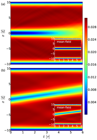
Figure 1: Time-evolution of the reduced one-body density $\rho_{1}(x;t)$ for $N=100$ bosons in a box of length $L=20\xi$ and a Lieb-Liniger parameter $\gamma=0.04$. The initial state resembles the properties of a black ($\beta=0.0$), a grey soliton ($\beta=0.5$) in (a) and (b), respectively. The calculations are performed with $M=4$ optimized SPFs. Insets show $M=1$ mean-field simulations. .

III.1 Reduced one-body density and contrast

All single-particle properties are described by the reduced one-body density operator $\hat{\rho}_{1}(t)={\rm tr}_{1}|\Psi_{t}\rangle\!\langle\Psi_{t}|$ being obtained by tracing out all bosons but a single one in the density operator of the $N$-body system. Firstly, let us compare the evolution of the reduced one-body density $\rho_{1}(x;t)=\langle x|\hat{\rho}_{1}(t)|x\rangle$ for a black and grey soliton. In Fig. 1, we present both mean-field and ML-MCTDHB calculations performed with $M=4$ optimized SPFs, to which we will refer as many-body simulations in the following as in contrast to the effective single-particle mean-field theory. One can clearly see that the applied density- and phase-engineering scheme generates stable solitons within the mean-field approximation, whereas the density minimum is becoming filled with atoms in the many-body simulations. This filling process appears to be slower in the case of a moving grey soliton compared to the black one. In both the many-body and the mean-field simulations, one clearly notices that our optimized density-engineering potential (II.3) allows for the generation of clean solitonic excitations: As a consequence of employing a Gaussian barrier of finite width, the black soliton is accompanied by quite some short

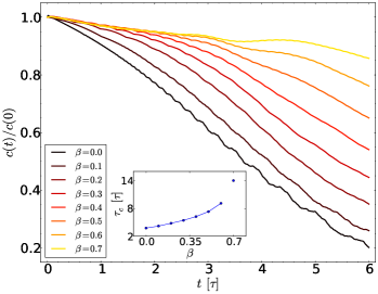
Figure 2: Time-evolution of the relative contrast $c(t)/c(0)$ for dark solitons of various soliton velocity to speed of sound ratios $\beta=u/s$. Inset: Contrast lifetime $\tau_{c}$ versus $\beta$. All other parameters as in Fig. 1.

wavelength phonons, which are visible as rays of density modulations in Fig. 1 (a). In contrast to this, only long wavelength phonon modes are marginally populated in the case of the optimized grey soliton engineering (Fig. 1 (b)).

Next we quantify the lifetime of the soliton contrast,

$$c(t)=\frac{{\rm max}\,\rho_{1}(x,0)-\rho_{1}(x^{s}_{t},t)}{{\rm max}\,\rho_{1}(x,0)+\rho_{1}(x^{s}_{t},t)},$$ (4)

where $x^{s}_{t}$ refers to the soliton position at time $t$ being defined as the position of the density minimum. To compare results for black and grey solitons, we define the contrast lifetime $\tau_{c}$ to be the time after which the relative contrast $c(t)/c(0)$ has dropped to $1/2$ (cf. also Mishmash and Carr (2009)). As the relative contrast is affected by some fluctuations due to phonons, we fit $f(t)=a+bt^{c}$ with $c>0$ to $c(t)/c(0)$ and extract $\tau_{c}=[(\frac{1}{2}-a)/b]^{\frac{1}{c}}$.

From Fig. 2, we may infer that the soliton contrast indeed lives the longer the closer $\beta$ approaches unity, which is consistent with the analytical prediction in Dziarmaga (2004). Moreover, the decay of the grey soliton relative contrast is approximately independent of $\beta$ for some time, which turns out to be longer for larger $\beta$. After that time, the relative contrast decays with a faster rate.

The inset of Fig. 2 depicts the contrast lifetime $\tau_{c}$ in dependence on $\beta$ showing that the lifetime of a grey soliton with $\beta=0.5$ is enhanced by a factor of $1.9$ compared the black soliton. The data for $\beta=0.6$, $\beta=0.7$ indicate that the lifetime can be increased much further. Yet we note that the lifetime values for $0.4<\beta<0.7$ refer to extrapolations to extend the converged results for a short time, while the individual data point for $\beta=0.7$ has been extrapolated because the soliton reaches the box boundary before $\tau_{c}$.

We finally remark that the dynamics of the relative contrast serves as a measure for the quality of the density-engineering: While the relative contrast decay is superimposed with only weak fluctuations for $0.1\leq\beta\leq 0.5$, stronger perturbations are visible for the black soliton as well as $\beta>0.5$. The perturbations for large $\beta$ values, which take place on a relatively long time-scale of about $2\tau$, raise from the fact that the soliton width separates less from the box length scale, which undermines the LDA underlying eq. (II.3). In the case of the black soliton, the short-time fluctuations are a consequence of the Gaussian potential barrier being not of optimal shape and, moreover, the choice for its width and height being a compromise between resembling the correct density profile and having a small condensate depletion at the same time.

III.2 Depletion and natural orbital analysis

In order to unravel the reduced one-body dynamics and to learn about the structure of the many-body wave function, we inspect the spectral decomposition of the reduced one-body density operator,

$$\hat{\rho}_{1}(t)=\sum_{i=1}^{M}\lambda_{i}(t)\,|\varphi_{i}(t)\rangle\!\langle\varphi_{i}(t)|,$$ (5)

defining the natural orbitals $|\varphi_{i}(t)\rangle$ and natural populations $\lambda_{i}(t)$ Löwdin (1955). First, we consider the depletion $d(t)=1-{\rm max}_{i}\,\lambda_{i}(t)\in[0,1]$ measuring how strongly the many-body wave function deviates from a perfect Bose-Einstein condensed state Penrose and Onsager (1956). In Fig. 3 (a), the evolution of $d(t)$ is compared for various values $\beta$. Initially, the maximal depletion of about $8.5\%$ is achieved for $\beta=0.0$ and $d(0)$ decreases with increasing $\beta$. However, we may also witness the impact of the $V_{\beta}(0)\sim 1/\beta^{2}$ divergence as $\beta$ tends to zero while the half-width-half-maximum of $V_{\beta}(x)$ saturates to a finite value: As we decrease $\beta$ linearly but keeping it still finite, the depletion $d(0)$ increases non-linearly, which is a consequence of $V_{\beta}(x)$ being optimal solely w.r.t. the (mean-field) density profile but not w.r.t. beyond mean-field properties such as depletion. Nevertheless, the initial many-body state is close enough to a perfectly condensed state for all considered $\beta$ values in order to initially resemble the important properties of mean-field dark solitons as we shall see below.

The subsequent dynamics of the depletion can be divided into two stages: Firstly, $d(t)$ stays quite constant for some time, which turns out to be the longer the larger $\beta$ is. Afterwards, a steep increase is followed with a slope increasing with decreasing $\beta$. Thereby, we observe that the greyer the soliton is the longer does it resemble mean-field characteristics such as conservation of contrast and low depletion.

In Fig. 3 (b), we present the natural populations $\lambda_{i}(t)$ for $\beta=0.0$ and $\beta=0.5$ as well as for a density- but not phase-engineered initial state, which is discussed in Sect. III.4. In principle, $M=4$ natural orbitals are available in our simulations, yet only two of them essentially contribute to the reduced one-body density operator and thereby to the total many-body wave function. The remaining two natural orbitals acquire natural populations of below $2\%$. Again, the dynamics consists of two stages: Firstly, the natural populations are stationary for a duration which prolongs with increasing $\beta$. Afterwards the most dominant natural orbital loses weight in favour for the second dominant one, which happens much faster for the black soliton compared to $\beta=0.5$ on the time-scales under consideration.

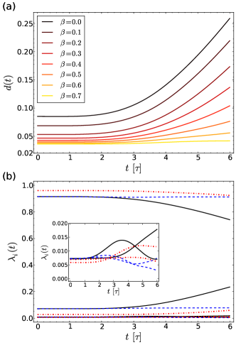
Figure 3: (a) Time evolution of the depletion $d(t)$ for various $\beta$. (b) Evolution of the natural populations $\lambda_{i}$ for $\beta=0.0$ (solid black lines) and $\beta=0.5$ (dashed dotted red lines). The blue dashed lines refer to the natural populations for an $\beta=0.0$ density- but not phase-engineered initial state. Inset: Close-up of the two least dominant natural populations. All other parameters as in Fig. 1.

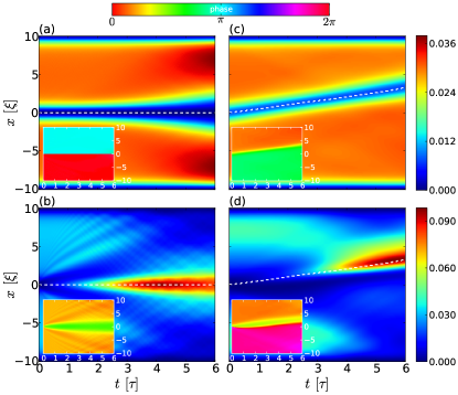
Figure 4: Comparison of the density evolution of the most and second dominant NO for a black soliton ((a) and (b)) and a grey soliton with $\beta=0.5$ ((c) and (d)). The instantaneous soliton positions $x^{s}_{t}$ defined as the minimum of $\rho_{1}(x;t)$ are depicted as white dashed lines. Insets: Phase profile of respective natural orbital. All other parameters as in Fig. 1.

Finally, we unravel the density- and phase-profiles of the two most dominant natural orbitals in Fig. 4. Clearly, the dominant natural orbital features solitonic characteristics such as the localized density minimum accompanied with an appropriate phase jump. In contrast to this, the second dominant natural orbital undergoes two stages of evolution. Firstly, the density is rearranged on a time-scale, on which also the depletion and the natural populations are stationary, i.e. until $t\sim 1.5\tau,...,3.5\tau$ for $\beta=0.0,...,0.7$. After this phase of the dynamics, the second dominant natural orbital has accumulated most of its density in the vicinity of the instantaneous density minimum of the dominant natural orbital. This accumulated density remains localized in the vicinity of the density dip of the dominant natural orbital even in the case of a moving grey soliton. In view of its natural population and density distribution, the second dominant natural orbital is mainly responsible for the filling of the one-body density depression - a result fully consistent with lattice simulations for black solitons in a box potential Mishmash et al. (2009) as well as a Bogoliubov treatment of black solitons in a harmonic trap, where the anomalous mode dominates the filling of the density minimum, e.g. Dziarmaga and Sacha (2002); Law et al. (2002).

In Fig. 4, we have moreover marked the position of the soliton allowing for identifying a crucial difference between black and grey solitons: For $\beta=0.0$, the many-body state has a well defined parity for all times, which translates into well defined parities of the natural orbitals and therefore leads to a perfectly symmetrically accumulated density of the second dominant natural orbital with respect to the soliton position. In contrast to this, the many-body state for $\beta>0$ can be shown to feature only a combined parity and time-reversal symmetry and, more importantly, the accumulated density of the second dominant natural orbital is not locally symmetric with respect to the instantaneous soliton position. In Sect. III.3, we will see that this asymmetry results in distinct two-body correlations. We remark that the degree of local asymmetry depends of the definition of the soliton position $x^{s}_{t}$: If we had defined $x^{s}_{t}$ as the minimum of the dominant natural orbital density $|\varphi_{1}(x;t)|^{2}$, the local asymmetry would be still present but slightly reduced. All statements in Sect. III.3 and III.4, which relate to the soliton position, hold qualitatively for both definitions of $x^{s}_{t}$ and we stick to $x^{s}_{t}$ being the position of the minimum of $\rho_{1}(x;t)$ as the latter is directly observable.

Before turning to the local two-body correlations, we comment on phonon excitation mechanisms: In the case of the black soliton, we observe that the even parity natural orbitals, i.e. the second and fourth one (not shown), are essentially carrying all phonon excitations visible in $\rho_{1}(x;t)$. These natural orbitals have been of odd parity before the phase-imprinting and possess a finite slope in the vicinity of $x=0$. Thus the phase-engineering creates a cusp at $x=0$, whose energy density is subsequently transported via phonons into the bulk as one can infer from the oscillatory density- and phase-modulations in Fig. 4 (b). Yet also the odd parity natural orbitals contribute to the phonons in $\rho_{1}(x;t)$ with, however, so minute weight that the density modulations are hardly observable in Fig. 4 (a). Here the phonon generation underlies a different mechanism: Having been of even parity before the phase-imprinting, odd parity natural orbitals initially feature a tiny but finite density at the phase-jump position $x=0$, which is transported into the bulk afterwards. It is conceivable that besides these two phonon generation mechanisms also the shape of $|\varphi_{i}(x;t)|^{2}$ in a finite vicinity of $x=0$ plays a role by storing excess energy when the density-engineering barrier is removed, which is then turned into phonon excitations. However, this argument should generically hold for all natural orbitals irrespectively of their parity and therefore we may regard this mechanism to be of minor importance if it is important at all. For $\beta=0.5$, phonons are hardly visible in the natural orbitals and therefore essentially absent in $\rho_{1}(x;t)$ as already discussed.

III.3 Two-body correlation analysis

As solitons are entities localized in space, we consider the local two-body correlation measure:

$$g_{2}(x_{1},x_{2};t)=\frac{\rho_{2}(x_{1},x_{2};t)}{\rho_{1}(x_{1};t)\rho_{1}(x_{2};t)},$$ (6)

which coincides with the diagonal of the second order coherence function defined by Glauber Glauber (1963). Here, we have introduced the two-body density $\rho_{2}(x_{1},x_{2};t)=\langle x_{1}x_{2}|\hat{\rho}_{2}(t)|x_{1}x_{2}\rangle$ with the reduced two-body density operator $\hat{\rho}_{2}(t)={\rm tr}_{2}|\Psi_{t}\rangle\!\langle\Psi_{t}|$ obtained by a partial trace over all but two bosons. Due to our normalization of $\rho_{2}(x_{1},x_{2};t)$ to unity, a perfectly condensed many-body state would lead to $g_{2}(x_{1},x_{2};t)=1$ everywhere. Finding $g_{2}(x_{1},x_{2};t)$ to be larger (smaller) than unity means that two bosons are found more (less) likely at the spots $(x_{1},x_{2})$ compared to statistical independence. Despite of the $g_{2}$-correlation function being one of the simplest observables sensitive to beyond mean-field properties, such correlations have not been studied in the context of dark solitons - except for the perturbative treatment with a different focus in Negretti et al. (2008). Besides its conceptual simplicity, the experimental accessibility via in situ density-density fluctuation measurements Hung et al. (2011); Endres et al. (2011); Cheneau et al. (2012); Endres et al. (2013); Jacqmin et al. (2011); Armijo et al. (2011); Armijo (2012) makes the $g_{2}$-correlation function attractive such that experimental interest in the correlation properties of dark solitons has already been triggered Armijo (2012). Due to the involved averaging process, probing beyond mean-field physics on the level of density fluctuations can turn out to be more robust than inspecting signatures becoming manifest only in single-shot $n$-body ($n\gg 2$) absorption image measurements as considered in e.g. Delande and Sacha (2014) - given a sufficient stability of the apparatus and imaging system, of course.

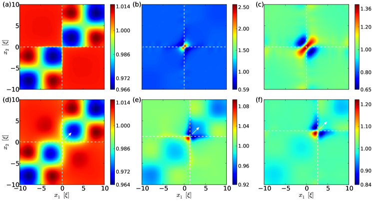
Figure 5: Two-body correlation function $g_{2}(x_{1},x_{2};t)$ for a black soliton (first row) and a grey soliton with $\beta=0.5$ (second) at times $t=0.0$ (first column), $t=2.5\tau$ (second) and $t=5\tau$ (third). Dashed lines refer to the instantaneous soliton position $x^{s}_{t}$ and the arrows indicate the direction of the soliton movement. All other parameters as in Fig. 1.

In Fig. 5, we compare the time evolution of the $g_{2}$-correlation measure for a black and a grey soliton initial state: Initially (Fig. 5 (a), (d)), $g_{2}(x_{1},x_{2};t=0)$ only marginally deviates from unity as expected for an initial state within the Thomas-Fermi mean-field regime. During the time evolution, however, the black and grey soliton establish quite distinct correlation patterns: Firstly focussing on the black soliton, the $g_{2}$-correlation function inherits the two-body reflection symmetry $g_{2}(-x_{1},-x_{2};t)=g_{2}(x_{1},x_{2};t)$ from the many-body wave function of well defined parity. Most of the detection events $(x_{1},x_{2})$ remain uncorrelated during the evolution, but pronounced correlations emerge in the vicinity of the soliton notch (Fig. 5 (b)): On the one hand side, we observe that a pair of bosons strongly bunches at the soliton position ($x_{1}=x_{2}=0$) or in the same flank of the soliton ($x_{1}x_{2}>0$). On the other hand, two bosons statistically avoid to be detected in different flanks of the soliton ($x_{1}x_{2}<0$). Thereby, the region around the soliton position where $g_{2}(x_{1},x_{2};t)$ features bunching is strongly squeezed on the off-diagonal $x_{2}=-x_{1}$ axis. At later times (Fig. 5 (c)), the $g_{2}$-function preserves its correlation pattern but its maximal value reduces by more than a factor $1.8$ compared to (Fig. 5 (b)). At the same time, the extent of the bunching (anti-bunching) region on the diagonal $x_{1}=x_{2}$ (off-diagonal $x_{1}=-x_{2}$) increases from about $1.7\xi$ ($1.0\xi$) to $3.0\xi$ ($2.2\xi$), which goes hand in hand with the widening of the minimum in the reduced one-body density (cf. Fig. 1 (a) and 4 (a)).

In the case of a grey soliton, the broken parity symmetry is imprinted in the evolution of the $g_{2}$-correlation function leading to quite a characteristic correlation pattern after a short time (Fig. 5 (e)): Most strikingly, the region where atom pairs occur bunched is localized in the soliton flank opposite to its direction of movement, i.e. $x_{1},x_{2}<x^{s}_{t}$, whereas atoms in the soliton flank pointing into its direction of motion are either slightly anti-bunched or uncorrelated. In fact, this displacement of the bunching region can be - at least partially - traced back to the local asymmetry of the second dominant natural orbital density w.r.t. the soliton position $x^{s}_{t}$: Focussing on the diagonal $x_{1}=x_{2}=x^{s}_{t}\pm\epsilon$, $\epsilon>0$ and on the vicinity of $x^{s}_{t}$ such that $\rho_{1}(x^{s}_{t}\pm\epsilon;t)\approx\lambda_{2}(t)|\varphi_{2}(x^{s}_{t}\pm\epsilon;t)|^{2}$ (cf. Fig. 4 (c)), one immediately sees that, for fixed two-body densities $\rho_{2}(x^{s}_{t}\pm\epsilon,x^{s}_{t}\pm\epsilon;t)$, the local asymmetry $|\varphi_{2}(x^{s}_{t}-\epsilon;t)|^{2}<|\varphi_{2}(x^{s}_{t}+\epsilon;t)|^{2}$ implies $g_{2}(x^{s}_{t}+\epsilon,x^{s}_{t}+\epsilon;t)<g_{2}(x^{s}_{t}-\epsilon,x^{s}_{t}-\epsilon;t)$ according to the definition (6).

Moreover, regions of anti-bunching emerge in the sectors $(x_{1},x_{2})\in\mathbb{R}^{2}$ with $x_{1/2}<x^{s}_{t}<x_{2/1}$, which are elongated towards the direction of motion of the soliton. In the overall correlation pattern, the maximal deviation of $g_{2}(x_{1},x_{2};t)$ from unity is with $\pm 8\%$ rather weak but increases at later times (Fig. 5 (f)). Furthermore, the anti-bunching regions become confined to the sectors $x_{1/2}<x^{s}_{t}<x_{2/1}$ then while an atom pair in the sector pointing into the soliton’s direction of movement, i.e. $x_{1},x_{2}>x^{s}_{t}$, turns out to be essentially uncorrelated. At even later times, the bunching region widens and shifts in the direction of movement such that it becomes approximately symmetric on the diagonal $x_{1}=x_{2}$ with respect to the soliton position $x^{s}_{t}$ (plot not shown). We note that the localization of the (anti-) bunching regions with respect to the soliton position does not depend on the choice for the definition of $x^{s}_{t}$ discussed in Sect. III.2.

In total, the maximal positive and negative deviations of $g_{2}(x_{1},x_{2};t)$ from unity are much smaller compared to the black soliton, which can be easily understood in terms of selection rules: While for $\beta=0$, the parity symmetry of the total wave function allows only to scatter atoms pairwise out of the most dominant natural orbital of odd parity into the even parity second most dominant NO (cf. also Dziarmaga et al. (2002); Mishmash and Carr (2009); Mishmash et al. (2009)), this process can also happen atom-wise in the case of a grey soliton. In view of the particular density distribution of the most and second most dominant natural orbital, two-body correlations have thereby to be quite pronounced for the black soliton, whereas relatively weaker correlations are possible for grey solitons.

In order to quantify the asymmetry of the correlation pattern in dependence on $\beta$, we define the position of the bunching centre as follows: Firstly, we introduce a bunching distribution within a disk of radius $R$ with centre $(x^{s}_{t},x^{s}_{t})$ as being proportional to the $g_{2}$-function minus one wherever it shows bunching:

$$p(x_{1},x_{2};t)\propto \left[\,g_{2}(x_{1},x_{2};t)-1\,\right]\;\times$$

$$\times\;\Theta(R-|{\bf x}-{\bf x}^{s}_{t}|)\;\Theta(g_{2}(x_{1},x_{2};t)-1).$$

Here, $\Theta(x)$ denotes the Heaviside step function and we use the abbreviations ${\bf x}=(x_{1},x_{2})$ as well as ${\bf x}^{s}_{t}=(x^{s}_{t},x^{s}_{t})$. In the following, we choose $R=4\xi$, which is sufficient for capturing the important correlation pattern. This probability distribution is used for defining the bunching centre ${\bf\bar{x}}_{t}$ as the expectation value of ${\bf x}$. Due to the particle exchange symmetry of the $g_{2}$-correlation function, both components of ${\bf\bar{x}}_{t}$ coincide and equal:

$$\bar{x}_{t}=\int{\rm d}x_{1}{\rm d}x_{2}\,x_{1}\,p(x_{1},x_{2};t).$$ (8)

For comparing the $\bar{x}_{t}$ dynamics for various $\beta$, we have performed a Galilean boost into the co-moving system of the soliton in Fig. 6 (a) depicting $\bar{x}_{t}-x^{s}_{t}$, which is proportional to bunching centre displacement from the soliton position in the $(x_{1},x_{2})$-plane, i.e. $|{\bf\bar{x}}_{t}-{\bf x}^{s}_{t}|=\sqrt{2}|\bar{x}_{t}-x^{s}_{t}|$. Within $0.5,...,2.5$ natural time units $\tau$ for $\beta=0.1,...,0.7$, the bunching centre $\bar{x}_{t}$ firstly moves away from the soliton opposite to its direction of motion with an approximately constant velocity being the faster the smaller $\beta$ (for $\beta>0$). This motion takes place with subsonic velocity as one can infer from a comparison with the trajectory $x(t)$ of a fictitious sonic excitation emitted opposite to the soliton direction of movement at $t=0$ from the soliton position $x(0)=0$. Importantly, this steady motion of the bunching centre lasts the longer the greyer the soliton is such that larger $\beta$ result in larger maximal displacements from the soliton position. After this phase of the dynamics, the displacement either features a maximum or stays for some time approximately at its maximal value before it decreases. This decrease reflects that the bunching centre becomes approximately symmetric with respect to the soliton position at even later times. Afterwards, we cannot make predictions for the further evolution since more optimized SPFs would be needed for ensuring convergence.

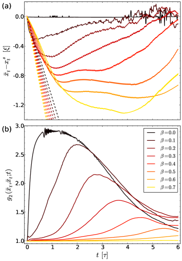
Figure 6: Analysis of the bunching centre $\bar{x}_{t}$ for various $\beta$: (a) Displacement of $\bar{x}_{t}$ with respect to instantaneous soliton position $x^{s}_{t}$. The dashed lines indicate the trajectories of a fictitious sonic excitation emitted at $t=0$ from the soliton position in negative $x$-direction for the various $\beta$, i.e. $x(t)-x^{s}_{t}=-\sqrt{g\rho_{\rm bulk}}\,t-x^{s}_{t}$, where the bulk density $\rho_{\rm bulk}$ is evaluated directly after the density-engineering at $t=0$. (b) The value of the two-body correlation function $g_{2}(\bar{x}_{t},\bar{x}_{t};t)$ at the bunching centre. The bunching distribution (III.3) is calculated for $R=4\xi$. All other parameters as in Fig. 1.

.

Although the term is definitely not proper in a strict sense, these findings suggest that the observed highly localized correlations feature a certain “inertia”: The phase-imprinting appears to give the density dip an instantaneous kick setting it thereby into motion. At the same time, bunching correlations emerge and drift the farer into the back of the soliton the stronger this kick is, i.e. the larger $\beta$. In order to test this picture, we have exerted a force on a grey soliton giving it dynamically a kick: By imposing an additional weak potential $V(x)=V_{0}\,[1-\tanh(x/l)]/2$ with $V_{0}>0$, $l=\mathcal{O}(\xi)$, we realize a bulk density profile $\propto[{\rm const.}-V(x)]$ featuring two distinct sound velocities $s_{l}<s_{r}$ in the left /right half space. We then initialize a grey soliton in the left half space ($x_{0}<0$ in (I)) moving to the right by means of the optimized density- and phase-engineering scheme introduced in Sect. II.3. Although $l=\mathcal{O}(\xi)$ results in a non-adiabatic change of the local density for the soliton (cf. e.g. Busch and Anglin (2000)), we have carefully checked that passing the step in the bulk density only leads to an acceleration of the soliton within the mean-field picture. The corresponding many-body simulation reveals that the bunching centre becomes drastically separated from the soliton position when passing $x=0$. Essentially, the bunching centre remains stuck in the vicinity of $x=0$ while decreasing in amplitude with time, giving thus further evidence for the aforementioned “inertia” of these localized correlations under kicks (plots not shown). We suspect that this “inertia” effect might be a consequence of the time-scales for the emergence and drift of these correlations being decoupled from the time-scales associated with the movement and acceleration of the density dip.

In Fig. 6 (b), we present the time evolution of the $g_{2}$-correlation function evaluated at the bunching centre, i.e. $g_{2}(\bar{x}_{t},\bar{x}_{t};t)$. For the black soliton, strong bunching correlations emerge almost instantaneously, which reflects the particular role of the parity induced selection rule, enforcing the dominant dynamical quantum depletion channel to take place pairwise, as well as the particular shape of the dominant and second dominant natural orbital for local two-body correlations. At about $t=1.0\tau$, the bunching correlations establish a maximum of approximately $2.9$ and afterwards these correlations decay again. We conjecture that this decay might be a precursor of a relaxation to a stationary state at later times. Qualitatively, the $g_{2}(\bar{x}_{t},\bar{x}_{t};t)$ follows essentially the same behaviour in the case of a grey soliton. However, the faster the soliton the longer does it take until noticeable correlations have built up. The build-up of correlations can last several natural time units $\tau$, i.e. is significantly longer compared to the black soliton. Moreover, the time when $g_{2}(\bar{x}_{t},\bar{x}_{t};t)$ becomes maximal turns out to be longer than the time needed for the bunching centre becoming maximally displaced from the soliton position. As expected from the previous observations, the maximum of $g_{2}(\bar{x}_{t},\bar{x}_{t};t)$ is smaller for larger $\beta$.

III.4 Role of phase-engineering

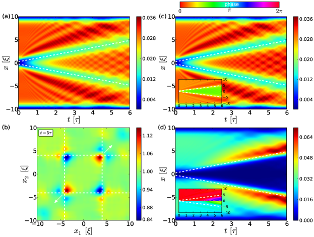
Figure 7: Evolution of a density-engineered initial state (no phase-imprinting is applied): Reduced one-body density $\rho_{1}(x;t)$ (a), two-body correlation function $g_{2}(x_{1},x_{2})$ at time $t=5\tau$ (b) as well as density of the dominant (c) and second dominant natural orbital (d) with corresponding phase profiles as insets. The corresponding natural populations are depicted in Fig. 3 (b). Dashed lines refer to the instantaneous soliton position $x^{s}_{t}$ obtained by linear regression of the position of the local $\rho_{1}(x;t)$ minima and the arrows indicate the direction of the soliton movement. All other parameters as in Fig. 1.

Having discussed the dynamics of a phase- and density-engineered solitonic initial state in detail, we finally investigate the role of the phase-imprinting procedure. For this purpose, we only apply the density-engineering scheme for a black soliton as described in Sect. II.3. As a result, we obtain an initial state with the very same natural population distribution as in the case of phase- and density-engineering. In contrast to the latter situation, the majority of atoms resides in a gerade rather than an ungerade orbital now, which constitutes an energetically more favourable situation. The subsequent many-body dynamics is summarized in Fig. 7.

In contrast to the phase- and density-engineered initial state, the density minimum now splits into two counter-propagating minima of constant velocities, which move through a background with phonon modes being excited much more intensively (Fig. 7 (a)). A mean-field simulation (plot not shown) essentially reveals the same density profile $\rho_{1}(x;t)$, which can be explained by the evolution of the natural populations in Fig. 3 (b): Quite in contrast to the density- and phase-engineered initial state, the natural populations essentially stay constant and, thus, the rather small initial depletion of about $8.5\%$ is retained. The density of the dominant natural orbital approximately resembles the full density profile $\rho_{1}(x;t)$ as expected while its phase profile features two phase jumps localized at the positions of these two minima (Fig. 7 (c)). Therefore, we may conclude that the density-engineering scheme creates two counter-propagating grey solitons with $|\beta|\approx 0.7$ in the single-particle state occupied by approximately $91.5\%$ of the atoms - as predicted for density-engineering in Gredeskul and Kivshar (1989); Gredeskul et al. (1990) within the mean-field theory and also experimentally observed in e.g. Dutton et al. (2001).

The remaining atoms essentially reside in the second dominant natural orbital being of odd parity, whose density appears as if being dragged to the box boundaries by the two grey solitons in the dominant natural orbital. Thereby, the region between the two solitons becomes depleted in density while density is accumulated in vicinity of the two density minima of the dominant natural orbital. Again, we can witness a local asymmetry of this accumulated density with respect to the position of the two grey solitons in the dominant natural orbital, which is a persistent feature for both definitions of the soliton position discussed in Sect. III.2. Moreover, we note that the phase of the second dominant natural orbital is approximately constant in domains $x\in[-L/2,0)$ and $x\in(0,L/2]$ so that this orbital hardly contributes to the probability current density $j(x;t)={\rm tr}(\hat{\jmath}(x)\hat{\rho}_{1}(t))$ with the current density operator $\hat{\jmath}(x)=\frac{1}{2}[\delta(x-\hat{x})\,\hat{p}+\hat{p}\,\delta(x-\hat{x})]$ and $\hat{x}$, $\hat{p}$ denoting the position and momentum operator, respectively. Thus, essentially only the phonon excitations being almost exclusively accommodated in the gerade dominant natural orbital as well as the mass counter-flow to the movement of the grey solitons in this orbital contribute to the current density $j(x;t)$.

Summarizing, all observations so far are consistent with our results on a single grey soliton, in particular the long lifetime of the contrast against decay via quantum fluctuations (cf. Fig. 2 (b), $\beta=0.7$). We finally address the question in Fig. 7 (b) whether also the $g_{2}$-correlation pattern can be understood as the sum of the correlation patterns of two counter-propagating grey solitons: Indeed, we find for $x_{1}$, $x_{2}$ in the vicinity of one and the same grey soliton that $g_{2}(x_{1},x_{2};t)$ resembles the peculiar locally asymmetric correlation pattern of bunching in the back of the soliton, anti-bunching of pairs of atoms being located in different flanks of the soliton and being uncorrelated ahead. Yet moreover, an additional, with respect to the soliton position non-local correlation structure has emerged. Denoting the position of e.g. the right moving grey soliton as $x^{s}_{t}$, we may state that bunching (anti-bunching) regions for $(x_{1},x_{2})$ in the vicinity of $(x^{s}_{t},x^{s}_{t})$ are turned into anti-bunching (bunching) regions under a parity transformation acting only on one of the two coordinates $(x_{1},x_{2})$: Finding one atom in each of the backs of the two solitons is statistically avoided while detecting one atom in each of the forward flanks of the two solitons is a rather uncorrelated event. Moreover, the probability of measuring one atom in the back flank of one soliton and another atom in the forward flank of the other soliton is slightly enhanced due to correlations. As a matter of fact, these non-local correlations between the solitons are a generic feature of parity symmetric many-body wave functions with essentially only two contributing natural orbitals and $g_{2}(0,0;t)\approx 1$ Krönke and Schmelcher (2015).

IV Conclusions and outlook

We have provided a systematic study of beyond mean-field signatures in black and, in particular, grey solitons. For this purpose, a robust, semi-analytically optimized density-engineering scheme has been developed, which in combination with phase-imprinting allows to cleanly generate grey solitons. In situations where the healing length can be increased above the optical diffraction limit, this preparation scheme is also of potential experimental relevance. We have demonstrated that the quantum fluctuations limited lifetime of dark solitons increases with their velocity. This is, in particular, intriguing as the variety of allowed incoherent scattering channels is larger for grey solitons compared to black ones of well defined party. The enhanced lifetime of grey solitons also manifests itself in a slower dynamical quantum depletion. The dark soliton decay takes place in a two step process: Firstly, the density of the second dominant natural orbital accumulates in the vicinity of the soliton while the depletion stays constant. Secondly, the population of this orbital increases significantly. Strikingly, the accumulated density of the second dominant natural orbital features a local asymmetry w.r.t. to the soliton position for grey solitons.

Dark solitons have the unique feature that quantum fluctuations induce spatially highly localized two-body correlations in the vicinity of the density minimum. While the zones of (anti-)bunching are distributed symmetrically around this minimum for a black soliton of well defined parity, the locally asymmetrically accumulated density of the second dominant natural orbital imprints itself in an asymmetric correlation pattern for grey solitons. In particular, we have shown that localized bunching correlations move to the backward flank of a grey soliton with subsonic velocity resulting in a bunching centre being the farer displaced from the soliton the faster the soliton moves through the bulk. Moreover, we have observed that these localized correlations have kind of a particle character in the sense that they feature a certain inertia under accelerations of the soliton. To unravel the underlying mechanism and sharpen the terminology for this phenomenology remains an interesting prospect for future works.

Finally, we have illuminated the role of the phase-imprinting: As within the mean-field approximation, density engineering alone results in pairs of counter-propagating grey solitons, which individually feature both the enhanced lifetime and peculiar localized correlation pattern of a single grey soliton. In addition, non-local two-body correlations between the two solitons emerge, which can be traced back to the parity symmetry, absent correlations at the parity-symmetry centre, $g_{2}(0,0;t)\approx 1$, and the fact that essentially only two natural orbitals contribute with significant weights Krönke and Schmelcher (2015). As a next step, it would be interesting to also study dark-bright solitons beyond the mean-field approximation in order to reveal possibly emerging inter-species correlations. Moreover, it is necessary to check the robustness of all these beyond mean-field signatures in the presence of decoherence and particle loss, which has been shown to significantly influence the properties of quantum bright matter wave solitons Weiss et al. (2014).

Appendix A Numerical parameters and convergence

The hard wall boundary conditions are implemented by a sine discrete variable representation (DVR) with $n=200$ grid points resulting in a grid spacing $\Delta x\approx 0.1\xi$ (cf. appendix of Beck et al. (2000)). Compared to the Bose-Hubbard approximation of a continuous system (cf. e.g. Schmidt and Fleischhauer (2007)), our sine DVR also considers next-to-nearest neighbour and higher order hopping processes. Due to the single-particle spectrum of the density-engineering Hamiltonian featuring pairs of quasi-degenerate states, it is only meaningful to consider an even number of SPFs when going beyond the mean-field approximation. We can efficiently afford for at most $M=4$ optimized SPFs when dealing with $N=100$ bosons resulting in $\sim 177.000$ number state configurations. By carefully comparing with $M=2$ simulations as well as with the results in Delande and Sacha (2014), we can ensure convergence at least up to times $t\sim 6.25\tau$, which is not long enough for relaxing to a uniform density profile but more than sufficient for the phenomena we are interested in. We emphasise that (ML-)MCTDHB gives a variationally optimized total wave function for any $M$.

References

- Remoissenet (1999) M. Remoissenet, Waves Called Solitons. Concepts and Experiments, 3rd ed. (Springer, 1999).
- Dauxois and Peyrard (2006) T. Dauxois and M. Peyrard, Physics of solitons (Cambridge University Press, 2006).
- Kevrekidis et al. (2008) P. G. Kevrekidis, D. J. Frantzeskakis, and R. Carretero-González, eds., Emergent Nonlinear Phenomena in Bose-Einstein Condensates. Theory and Experiment, Springer Series on Atomic, Optical, and Plasma Physics, Vol. 45 (Springer Berlin / Heidelberg, 2008).
- Frantzeskakis (2010) D. J. Frantzeskakis, J. Phys. A 43, 213001 (2010).
- Tsuzuki (1971) T. Tsuzuki, J. Low. Temp. Phys. 4, 441 (1971).
- Pethick and Smith (2008) C. J. Pethick and H. Smith, Bose-Einstein Condensates in Dilute Gases, 2nd ed. (Cambridge University Press, 2008).
- Muryshev et al. (2002) A. Muryshev, G. V. Shlyapnikov, W. Ertmer, K. Sengstock, and M. Lewenstein, Phys. Rev. Lett. 89, 110401 (2002).
- Gangardt and Kamenev (2010) D. M. Gangardt and A. Kamenev, Phys. Rev. Lett. 104, 190402 (2010).
- Cockburn et al. (2011) S. P. Cockburn, H. E. Nistazakis, T. P. Horikis, P. G. Kevrekidis, N. P. Proukakis, and D. J. Frantzeskakis, Phys. Rev. A 84, 043640 (2011).
- Brand and Reinhardt (2002) J. Brand and W. P. Reinhardt, Phys. Rev. A 65, 043612 (2002).
- Becker et al. (2013) C. Becker, K. Sengstock, P. Schmelcher, P. G. Kevrekidis, and R. Carretero-González, New J. Phys. 15, 113028 (2013).
- Ku et al. (2014) M. J. H. Ku, W. Ji, B. Mukherjee, E. Guardado-Sanchez, L. W. Cheuk, T. Yefsah, and M. W. Zwierlein, Phys. Rev. Lett. 113, 065301 (2014).
- Donadello et al. (2014) S. Donadello, S. Serafini, M. Tylutki, L. P. Pitaevskii, F. Dalfovo, G. Lamporesi, and G. Ferrari, Phys. Rev. Lett. 113, 065302 (2014).
- Muñoz Mateo and Brand (2014) A. Muñoz Mateo and J. Brand, Phys. Rev. Lett. 113, 255302 (2014).
- Dagnino et al. (2009) D. Dagnino, N. Barberán, M. Lewenstein, and J. Dalibard, Nature 5, 431 (2009).
- Weiner et al. (2014) S. E. Weiner, M. C. Tsatsos, L. S. Cederbaum, and A. U. J. Lode, arXiv:1409.7670 (2014).
- Tsatsos and Lode (2014) M. C. Tsatsos and A. U. J. Lode, arXiv:1410.0414 (2014).
- Wells et al. (2014) T. Wells, A. U. J. Lode, V. S. Bagnato, and M. C. Tsatsos, arXiv:1410.2859 (2014).
- Kulish et al. (1976) P. P. Kulish, S. V. Manakov, and L. D. Faddeev, Theor. Math. Phys. 28, 615 (1976).
- Ishikawa and Takayama (1980) M. Ishikawa and H. Takayama, J. Phys. Soc. Jpn. 49, 1242 (1980).
- Kanamoto et al. (2010) R. Kanamoto, L. D. Carr, and M. Ueda, Phys. Rev. A 81, 023625 (2010).
- Sato et al. (2012a) J. Sato, R. Kanamoto, E. Kaminishi, and T. Deguchi, Phys. Rev. Lett. 108, 110401 (2012a).
- Sato et al. (2012b) J. Sato, R. Kanamoto, E. Kaminishi, and T. Deguchi, arXiv:1204.3960 (2012b).
- Wadkin-Snaith and Gangardt (2012) D. C. Wadkin-Snaith and D. M. Gangardt, Phys. Rev. Lett. 108, 085301 (2012).
- Astrakharchik and Pitaevskii (2013) G. E. Astrakharchik and L. P. Pitaevskii, EPL 102, 30004 (2013).
- Draxler et al. (2013) D. Draxler, J. Haegeman, T. J. Osborne, V. Stojevic, L. Vanderstraeten, and F. Verstraete, Phys. Rev. Lett. 111, 020402 (2013).
- Karpiuk et al. (2015) T. Karpiuk, T. Sowiński, M. Gajda, K. Rzążewski, and M. Brewczyk, Phys. Rev. A 91, 013621 (2015).
- Lieb and Liniger (1963) E. H. Lieb and W. Liniger, Phys. Rev. 130, 1605 (1963).
- Lieb (1963) E. H. Lieb, Phys. Rev. 130, 1616 (1963).
- Burger et al. (1999) S. Burger, K. Bongs, S. Dettmer, W. Ertmer, K. Sengstock, A. Sanpera, G. V. Shlyapnikov, and M. Lewenstein, Phys. Rev. Lett. 83, 5198 (1999).
- Dziarmaga et al. (2002) J. Dziarmaga, Z. P. Karkuszewski, and K. Sacha, Phys. Rev. A 66, 043615 (2002).
- Dziarmaga and Sacha (2002) J. Dziarmaga and K. Sacha, Phys. Rev. A 66, 043620 (2002).
- Law et al. (2002) C. K. Law, P. T. Leung, and M.-C. Chu, J. Phys. B: At. Mol. Opt. Phys. 35, 3583 (2002).
- Dziarmaga et al. (2003) Z. Dziarmaga, Z. P. Karkuszewski, and K. Sacha, J. Phys. B: At. Mol. Opt. Phys. 36, 1217 (2003).
- Law (2003) C. K. Law, Phys. Rev. A 68, 015602 (2003).
- Dziarmaga and Sacha (2006) J. Dziarmaga and K. Sacha, J. Phys. B: At. Mol. Opt. Phys. 39, 57 (2006).
- Dziarmaga (2004) J. Dziarmaga, Phys. Rev. A 70, 063616 (2004).
- Mishmash and Carr (2009) R. V. Mishmash and L. D. Carr, Phys. Rev. Lett. 103, 140403 (2009).
- Mishmash et al. (2009) R. V. Mishmash, I. Danshita, C. W. Clark, and L. D. Carr, Phys. Rev. A 80, 053612 (2009).
- Martin and Ruostekoski (2010) A. D. Martin and J. Ruostekoski, Phys. Rev. Lett. 104, 194102 (2010).
- Delande and Sacha (2014) D. Delande and K. Sacha, Phys. Rev. Lett. 112, 040402 (2014).
- Dziarmaga et al. (2010) J. Dziarmaga, P. Deuar, and K. Sacha, Phys. Rev. Lett. 105, 018903 (2010).
- Mishmash and Carr (2010) R. V. Mishmash and L. D. Carr, Phys. Rev. Lett. 105, 018904 (2010).
- Meyrath et al. (2005) T. P. Meyrath, F. Schreck, J. L. Hanssen, C.-S. Chuu, and M. G. Raizen, Phys. Rev. A 71, 041604 (2005).
- Henderson et al. (2009) K. Henderson, C. Ryu, C. MacCormick, and M. G. Boshier, New J. Phys. 11, 043030 (2009).
- Gaunt et al. (2013) A. L. Gaunt, T. F. Schmidutz, I. Gotlibovych, R. P. Smith, and Z. Hadzibabic, Phys. Rev. Lett. 110, 200406 (2013).
- Olshanii (1998) M. Olshanii, Phys. Rev. Lett. 81, 938 (1998).
- Lieb et al. (2003) E. H. Lieb, R. Seiringer, and J. Yngvason, Phys. Rev. Lett. 91, 150401 (2003).
- Vidal (2003) G. Vidal, Phys. Rev. Lett. 91, 147902 (2003).
- Krönke et al. (2013) S. Krönke, L. Cao, O. Vendrell, and P. Schmelcher, New J. Phys. 15, 063018 (2013).
- Cao et al. (2013) L. Cao, S. Krönke, O. Vendrell, and P. Schmelcher, J. Chem. Phys. 139, 134103 (2013).
- Streltsov et al. (2007) A. I. Streltsov, O. E. Alon, and L. S. Cederbaum, Phys. Rev. Lett. 99, 030402 (2007).
- Alon et al. (2008) O. E. Alon, A. I. Streltsov, and L. S. Cederbaum, Phys. Rev. A 77, 033613 (2008).
- Carr et al. (2001) L. D. Carr, J. Brand, S. Burger, and A. Sanpera, Phys. Rev. A 63, 051601 (2001).
- Löwdin (1955) P.-O. Löwdin, Phys. Rev. 97, 1474 (1955).
- Penrose and Onsager (1956) O. Penrose and L. Onsager, Phys. Rev. 104, 576 (1956).
- Glauber (1963) R. J. Glauber, Phys. Rev. 130, 2529 (1963).
- Negretti et al. (2008) A. Negretti, C. Henkel, and K. Mølmer, Phys. Rev. A 78, 023630 (2008).
- Hung et al. (2011) C.-L. Hung, X. Zhang, T. S.-K. Ha, L.-C. and, N. Gemelke, and C. Chin, New J. Phys. 13, 075019 (2011).
- Endres et al. (2011) M. Endres, M. Cheneau, T. Fukuhara, C. Weitenberg, P. Schauß, C. Gross, L. Mazza, M. C. Bañuls, L. Pollet, I. Bloch, and S. Kuhr, Science 334, 200 (2011).
- Cheneau et al. (2012) M. Cheneau, P. Barmettler, D. Poletti, M. Endres, P. Schauß, T. Fukuhara, C. Gross, I. Bloch, C. Kollath, and S. Kuhr, Nature 481, 484 (2012).
- Endres et al. (2013) M. Endres, M. Cheneau, T. Fukuhara, C. Weitenberg, P. Schauß, C. Gross, L. Mazza, M. C. Bañuls, L. Pollet, I. Bloch, and S. Kuhr, Appl. Phys. B 113, 27 (2013).
- Jacqmin et al. (2011) T. Jacqmin, J. Armijo, T. Berrada, K. V. Kheruntsyan, and I. Bouchoule, Phys. Rev. Lett. 106, 230405 (2011).
- Armijo et al. (2011) J. Armijo, T. Jacqmin, K. Kheruntsyan, and I. Bouchoule, Phys. Rev. A 83, 021605 (2011).
- Armijo (2012) J. Armijo, Phys. Rev. Lett. 108, 225306 (2012).
- Walczak and Anglin (2011) P. B. Walczak and J. R. Anglin, Phys. Rev. A 84, 013611 (2011).
- Busch and Anglin (2000) T. Busch and J. R. Anglin, Phys. Rev. Lett. 84, 2298 (2000).
- Gredeskul and Kivshar (1989) S. A. Gredeskul and Y. S. Kivshar, Phys. Rev. Lett. 62, 977 (1989).
- Gredeskul et al. (1990) S. A. Gredeskul, Y. S. Kivshar, and M. V. Yanovskaya, Phys. Rev. A 41, 3994 (1990).
- Dutton et al. (2001) Z. Dutton, M. Budde, C. Slowe, and L. V. Hau, Science 293, 663 (2001).
- Krönke and Schmelcher (2015) S. Krönke and P. Schmelcher, arXiv:1501.07886 (2015).
- Weiss et al. (2014) C. Weiss, S. A. Gardiner, and H.-P. Breuer, arXiv:1407.7633 (2014).
- Beck et al. (2000) M. H. Beck, A. Jäckle, G. A. Worth, and H.-D. Meyer, Phys. Rep. 324, 1 (2000).
- Schmidt and Fleischhauer (2007) B. Schmidt and M. Fleischhauer, Phys. Rev. A 75, 021601 (2007).