The other optimal Stokes drag profile

Abstract

The lowest drag shape of fixed volume in Stokes flow has been known for some $40$ years. It is front-back symmetric and similar to an American football with ends tangent to a cone of $60^{\circ}$. The analogous convex axisymmetric shape of fixed surface area, which may be of interest for particle design in chemistry and colloidal science, is characterized in this paper. This “other” optimal shape has a surface vorticity proportional to the mean surface curvature, which is used with a local analysis of the flow near the tip to show that the front and rear ends are tangent to a cone of angle $30.8^{\circ}$. Using the boundary element method, we numerically represent the shape by expanding its tangent angle in terms decaying odd Legendre modes, and show that it has $11.3\%$ lower drag than a sphere of equal surface area, significantly more pronounced than for the fixed-volume optimal.

1 Introduction

Design optimisation is observed throughout nature, and it has long been used in the private sector for better and more efficient design. Many industries, particularly aeronautics (Jameson et al., 1998; Alonso et al., 2009) and ship design (Campana et al., 2009), use fluid dynamical considerations when optimising shapes (Mohammadi & Pironneau, 2004), such as minimising drag or maximising lift. These optimisations are usually subject to constraints, for instance a ship might need to have a fixed volume, or certain shapes might be too costly to engineer. In nature, too, optimisation is subject to physical constraints; for example, the beat patterns of spermatozoa (Pironneau & Katz, 1974; Lauga & Eloy, 2013) and cilia (Osterman & Vilfan, 2011; Eloy & Lauga, 2012) are subject to energetic constraints on the molecular motors responsible for the motion. Similarly the shapes of squirming microorganisms correspond closely to those minimising power dissipation subject to a maximum curvature (Vilfan, 2012). Inspired by nature, shape optimisation can be used to improve the design of biomimetic artificial swimmers (Keaveny et al., 2013).

In a classical paper, Pironneau (1973) used a variational approach to show that, in the absence of inertia, the lowest drag shape of fixed volume is front-back symmetric with constant vorticity on its surface. Furthermore, the front and rear of the shape taper into cones of semi-cone angle $60^{\circ}$. This shape was then computed numerically by Bourot (1974) by minimising the drag among a finite family of shapes. Pironneau’s optimal profile has subsequently been observed in the explosively-launched spores of ascomycete fungi (Roper et al., 2008). The constraint of fixed volume is appropriate in this biological case, as a certain amount of material is required in order to generate a new organism.

Recently, mechanical optimisations have begun to be examined for more efficient drug delivery, using material rather than chemical properties to achieve specific effects (Champion et al., 2007; Mitragotri & Lahann, 2009; Petros & DeSimone, 2010). Varying the shape, size, mechanical and surface properties properties of drugs can significantly impact drug-delivery processes such as phagocytosis (Champion & Mitragotri, 2006), whereby macrophages engulf solid particles. Gratton et al. (2008) showed that microscopic, slender rod-like particles with aspect ratio three, corresponding to eccentricity $e=0.9428$, were subsumed four times faster than spherical particles of equal volume.

A potentially important constraint for designer drug delivery, and also biomimetic microrobots, is fixed particle surface area. Indeed, surface area affects diffusion rates, is associated with toxicity (Monteiller et al., 2007), and is important in setting the rate of production of reactants for catalysis and chemical reaction. In this study, we determine the analogous fixed-surface-area shape to Pironneau’s fixed-volume optimal; that is, the convex, axisymmetric shape that minimises drag subject to fixed surface area. These constraints restrict us to a family of simply manufactured shapes resembling Pironneau’s optimum, and specifically rule out fractal-like shapes of finite surface area folded into a very small space. We derive the fixed-surface-area shape numerically using a representation whereby its tangent angle is described by a very small number of odd Legendre modes, together with a local analysis of the equations of fluid motion. We show that this “other” optimal shape is almost twice as slender as the fixed-volume shape, has a surface vorticity square proportional to the mean surface curvature (Pironneau, 1973; Bourot, 1974) and near either end is locally conical about an angle of $30.8^{\circ}$.

2 Mathematical analysis

Two aspects of the optimisation problem are amenable to an analytical approach, namely the optimality condition and a local shape analysis near either end of the body.

2.1 Optimality condition

We begin by deriving the shape’s optimality condition, following Pironneau (1973). In Newtonian flows at microscopic scales, the fluid flow velocity $\mathbf{u}$ driven by a body force per unit volume $\mathbf{F}$ is governed by the Stokes flow equations,

$$\boldsymbol{\nabla}p=\mu\nabla^{2}\mathbf{u}+\mathbf{F},\quad\boldsymbol{\nabla}\cdot\mathbf{u}=0,$$ (1)

with pressure $p$ and viscosity $\mu$. Consider a shape $S$ described by ${\bf x}$ translating in this fluid at a fixed speed ${\bf U}$ in the absence fluid body forces ($\mathbf{F}=\bf 0$). In the reference frame of the body the velocity satisfies the no-slip boundary condition as ${\bf u}({\bf x})=\bf 0$ and ${\bf u}=-{\bf U}$ at infinity. We want to find the shape minimizing the drag. The rate of working of the drag is equal to the rate of viscous dissipation in the fluid, and so we wish to minimize

$$D=2\mu\int_{V}e_{ij}e_{ij}{\rm d}V,$$ (2)

where $V$ refers to the volume outside of the shape and $e_{ij}=({\partial}u_{i}/{\partial}x_{j}+{\partial}u_{j}/{\partial}x_{i})/2$.

Perturbing $S$ into a new shape described by ${\bf x}+\alpha{\bf n}$, where ${\bf n}$ is the normal to the surface and $\alpha$ is assumed to be a small length everywhere, we denote the resulting change in the velocity field around the shape by $\delta{\bf u}$. The change in the dissipation is given by

$$\delta D=\mu\int_{V}\left(\frac{{\partial}u_{i}}{{\partial}x_{j}}+\frac{{\partial}u_{j}}{{\partial}x_{i}}\right)\left(\frac{{\partial}\delta u_{i}}{{\partial}x_{j}}+\frac{{\partial}\delta u_{j}}{{\partial}x_{i}}\right){\rm d}V.$$ (3)

Using integration by parts and symmetries in the indices we obtain

$$\delta D=-2\mu\int_{V}\delta u_{i}\left(\frac{{\partial}^{2}u_{i}}{{\partial}x_{j}{\partial}x_{j}}+\frac{{\partial}^{2}u_{j}}{{\partial}x_{i}{\partial}x_{j}}\right){\rm d}V+2\mu\int_{S}\delta u_{j}\left(\frac{{\partial}u_{i}}{{\partial}x_{j}}+\frac{{\partial}u_{j}}{{\partial}x_{i}}\right)n_{i}{\rm d}S.$$ (4)

Since $\nabla\cdot{\bf u}=0$, we have identically ${{\partial}_{j}{\partial}_{i}u_{j}}=0$. The first term in the first integral in equation (4) is the Laplacian of the velocity field, which we know from equation (1) in the absence of body forces is given by $\mu{{\partial}_{j}{\partial}_{j}u_{i}}={{\partial}_{i}p}.$ Furthermore, a Taylor expansion of the no-slip boundary condition $({\bf u}+\delta{\bf u})({\bf x}+\alpha{\bf n})=\bf 0$ allows us to obtain

$$\delta{\bf u}({\bf x})=-\alpha\frac{{\partial}{\bf u}}{{\partial}n}\cdot$$ (5)

With these two results, equation (4) simplifies to

$$\delta D=-2\int_{V}\delta u_{i}\frac{{\partial}p}{{\partial}x_{i}}{\rm d}V-2\mu\int_{S}\alpha\frac{{\partial}u_{j}}{{\partial}n}\left(\frac{{\partial}u_{i}}{{\partial}x_{j}}+\frac{{\partial}u_{j}}{{\partial}x_{i}}\right)n_{i}{\rm d}S.$$ (6)

Using integration by parts, the first integral in equation (6) becomes

$$\int_{V}-p\frac{{\partial}\delta u_{i}}{{\partial}x_{i}}{\rm d}V+\int_{S}p\delta u_{i}n_{i}{\rm d}S.$$ (7)

The first term in equation (7) is zero because the perturbation flow is divergence free, while the second term is zero because of equation (5) and the divergence-free condition. Because of the no-slip boundary condition for ${\bf u}$ and the fact that it is divergence free, the last integral in equation (6) can be further simplified to

$$\delta D=-2\mu\int_{S}\alpha\frac{{\partial}u_{j}}{{\partial}n}\frac{{\partial}u_{j}}{{\partial}n}{\rm d}S=-2\mu\int_{S}\alpha\bigg{|}\frac{{\partial}{\bf u}}{{\partial}n}\bigg{|}^{2}{\rm d}S.$$ (8)

In the fixed-surface-area case, we consider a cost function of the form

$$J=D+\lambda\left(\int_{S}{\rm d}S-S_{0}\right),$$ (9)

where $\lambda$ is the Lagrange multiplier enforcing the constraint of fixed surface area, $S=S_{0}$. Variations in $S$ arising from the perturbation to the shape are given by $2\int\kappa\alpha{\rm d}S$ where $\kappa$ is the mean surface curvature, and thus the perturbation to $J$ is given by

$$\delta J=\delta D+\lambda\delta S=-2\mu\int_{S}\alpha\bigg{|}\frac{{\partial}{\bf u}}{{\partial}n}\bigg{|}^{2}{\rm d}S+2\lambda\int_{S}\kappa{\alpha}{\rm d}S=2\int_{S}\alpha\left(-\mu\bigg{|}\frac{{\partial}{\bf u}}{{\partial}n}\bigg{|}^{2}+\lambda\kappa\right){\rm d}S.$$ (10)

By setting $\delta J=0$, the optimality condition is then

$$|\partial\mathbf{u}/\partial{{n}}|^{2}\propto\kappa,$$ (11)

where the first term can also be seen as the norm squared of the surface vorticity. Note that in the fixed-volume case, the cost function is $J=D+\lambda(V-V_{0})$, and since $\delta V=\int\alpha{\rm d}S$, the optimal shape has constant surface vorticity (Pironneau, 1973).

2.2 Local analysis

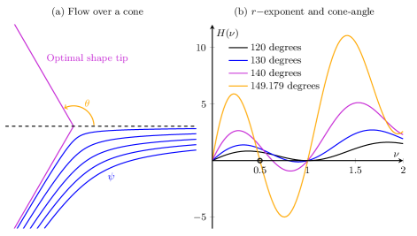
Figure 1: (a) Flow over the vertex of a cone illustrating the streamfunction for the minimal drag fixed volume case of $\theta_{0}=120^{\circ}$; (b) The function $H(\nu)$ in equation (17) for a selection of cone angles, highlighting the minimal drag fixed surface area case of $\theta_{0}=149.179^{\circ}$.

As shown by Pironneau (1973) and Bourot (1974), optimal shapes have pointy, American football-like ends. The second aspect of the optimisation problem which can be treated analytically is a derivation of the optimal angle at either end of the locally-conical shape.

We consider a conical shape and describe the axisymmetric flow around it using spherical coordinates $(r,\theta)$ with $r$ measured from the tip and $\theta$ from the axis of symmetry in the fluid (figure 1a). The cone is assumed to be located at $\theta=\theta_{0}$, where $\theta_{0}$ may be $90^{\circ}$ in the case of a blunt body, and the goal of the analysis is to derive the value of $\theta_{0}$ consistent with the optimality condition. Locally around the cone, the streamfunction $\psi(r,\theta)$ is expected to take the asymptotic form $\psi=r^{n}f(\theta)$. The equations and boundary conditions satisfied by the streamfunction are

$$E^{2}(E^{2}\psi)=0,\,\,E^{2}=\frac{\partial^{2}}{\partial r^{2}}+\frac{\sin\theta}{r^{2}}\frac{\partial}{\partial\theta}\left[\frac{1}{\sin\theta}\frac{\partial}{\partial\theta}\right],\,\,\left.\frac{\partial\psi}{\partial\theta}\right|_{\theta_{0}}=0,\,\,\psi(\theta_{0})=\psi(0)=0.$$ (12)

In the case of fixed volume, the optimality condition of constant surface vorticity yields

$$|\partial\mathbf{u}/\partial n|=|E^{2}\psi/r\sin\theta|=\mbox{const.}\quad\Rightarrow\quad n=3.$$ (13)

The solution for $f(\theta)$ given in Pironneau (1973) does not, however, satisfy the condition that $\psi(\theta_{0})=0$ (equation 12), and we re-derive it here. Plugging the ansatz $\psi=r^{3}f(\theta)$ into equation (12) leads to the ordinary differential equation

$$f^{\prime\prime}-\cot\theta f^{\prime}+6f=A\cos\theta+B.$$ (14)

Together with the particular solution, the full solution is then $\psi=cr^{3}(at+bt^{3}+1)$ for $t=\cos\theta$. In order to enforce the boundary conditions, the constants must be $a=-3/2t_{0}$, $b=1/2t_{0}^{3}$. Finally, since the streamline along $\theta=0$ (or $t=1$) is split by the cone, we require $f(0)=0$ i.e.

$$\frac{1}{2t_{0}^{3}}-\frac{3}{2t_{0}}+1=0\quad\Rightarrow\quad(t_{0}+1/2)(t_{0}-1)^{2}=0,$$ (15)

and therefore $t_{0}=-1/2$ or $\theta_{0}=120^{\circ}$. The optimal fixed-volume body thus has locally conical ends with a semi-angle $\theta_{sc}=60^{\circ}$, agreeing with the result of Pironneau (1973). The streamlines associated with this flow are displayed in figure 1a.

For the fixed-surface-area shape, the optimality condition depends on the mean curvature $\kappa$ of the surface (equation 11). Note that this means we expect the vorticity on the surface of our optimal shape to diverge towards its front and rear ends. At the conical tip, $\kappa\propto 1/r$, and following the same local analysis, this condition may be written

$$r|\partial\mathbf{u}/\partial n|^{2}=r|E^{2}\psi/r\sin\theta|^{2}=\mbox{const.}\quad\Rightarrow\quad n=5/2.$$ (16)

In order to derive the cone angle corresponding this value $n=5/2$, we turn to Wakiya (1976) who considered Stokes flows near the tip of rigid bodies. In particular, Wakiya showed that, for a given cone angle $\theta_{0}$, the exponent $n$ of the streamfunction satisfying (12) is given by the first nontrivial root (ie, $\nu\neq 0,1$) of

$$H(\nu)=P_{\nu}(t_{0})\left[t_{0}P^{\prime\prime}_{\nu}(t_{0})+P^{\prime}_{\nu}(t_{0})\right]-t_{0}\left[P^{\prime}_{\nu}(t_{0})\right]^{2},$$ (17)

where $\nu+2=n$ and $P_{\nu}$ is the Legendre function of the first kind of, possibly fractional, degree $\nu$. The function $H(\nu)$ is plotted for cone angles in figure 1b. The fixed-volume shape is the special case where $\nu=1$ is a double root of equation (17). In the case of a fixed-surface constraint, we have $\nu=1/2$, and we can numerically invert equation (17) to obtain the corresponding value of $t_{0}$. This is illustrated in figure 1b and we obtain $\theta_{0}=149.179^{\circ}$ in our coordinate system, corresponding to a semi-cone angle of

$$\theta_{sc}\approx 30.8^{\circ}.$$ (18)

We thus expect to obtain a more slender optimal shape than in the fixed-volume case.

3 Numerical shape optimisation

We now proceed with a computational approach in order to derive the optimal shape and confirm the validity of our local analysis. The fundamental solution to the Stokes flow equations (1) driven point a point force $\mathbf{f}\delta(\mathbf{x}-\mathbf{y})$ located at $\mathbf{y}$ is given by the stokeslet tensor $S_{ij}(\mathbf{x},\mathbf{y})$,

$$u_{i}(\mathbf{x})=S_{ij}(\mathbf{x},\mathbf{y})f_{j},\quad S_{ij}(\mathbf{x},\mathbf{y})=\frac{1}{8\pi}\left(\frac{\delta_{ij}}{r}+\frac{r_{i}r_{j}}{r^{3}}\right),$$ (19)

where $r_{i}=x_{i}-y_{i}$ and $r^{2}=r_{1}^{2}+r_{2}^{2}+r_{3}^{2}$. For axisymmetric flow, the Green’s function corresponding to a ring of point forces $M_{\alpha,\beta}(\mathbf{x}-\mathbf{x}_{0})$ can then be obtained by integrating the Stokeslet in the azimuthal direction (Pozrikidis, 1992),

$$M_{xx}=2k\left(\frac{\sigma_{0}}{\sigma}\right)^{1/2}\left(F+\frac{\hat{x}^{2}}{\hat{r}^{2}}E\right),\quad M_{x\sigma}=-k\frac{\hat{x}}{\sigma_{0}\sigma^{1/2}}\left[F-(\sigma^{2}-\sigma_{0}^{2}+\hat{x}^{2})\frac{E}{\hat{r}^{2}}\right],$$

$$M_{\sigma x}=k\frac{\hat{x}}{\sigma}\left(\frac{\sigma_{0}}{\sigma}\right)^{1/2}\left[F+(\sigma^{2}-\sigma_{0}^{2}-\hat{x}^{2})\frac{E}{\hat{r}^{2}}\right],$$ (20)

$$M_{\sigma\sigma}=\frac{k}{\sigma_{0}\sigma}\left(\frac{\sigma_{0}}{\sigma}\right)^{1/2}\left\{(\sigma_{0}^{2}+\sigma^{2}+2\hat{x}^{2})F-\left[2\hat{x}^{4}+3\hat{x}^{2}(\sigma_{0}^{2}+\sigma^{2})+(\sigma^{2}-\sigma_{0}^{2})^{2}\right]\frac{E}{\hat{r}^{2}}\right\}.$$

Here, $F$ and $E$ are complete elliptic integrals of the first kind of argument $k$,

$$F(k)=\int_{0}^{\pi/2}\frac{\mathrm{d}\omega}{(1-k^{2}\cos^{2}\omega)^{1/2}},\quad E(k)=\int_{0}^{\pi/2}(1-k^{2}\cos^{2}\omega)^{1/2}\,\mathrm{d}\omega,\quad$$ (21)

where $k^{2}={4\sigma\sigma_{0}}/[{\hat{x}^{2}+(\sigma+\sigma_{0})^{2}}]$, while $\hat{x}=x-x_{0}$ and $r^{2}=\hat{x}^{2}+(\sigma-\sigma_{0})^{2}$ are axial and radial coordinates $(x,\sigma)$.

The Newtonian fluid flow around our axisymmetric body can then be reduced to a boundary integral of ring forces taken over the meridional plane,

$$u_{\alpha}(\mathbf{y})=\frac{1}{8\pi}\int_{C}M_{\alpha\beta}(\mathbf{x},\mathbf{y})f_{\beta}(\mathbf{y})\,\mathrm{d}l,$$ (22)

where the double layer potential has been eliminated (rigid-body motion). The meridional plane of the rigid body is discretised into straight-line segments of constant force per unit length; i.e. the components $f_{x},f_{\sigma}$ in equation (22) are constant over each element $s_{i}$. The velocity of the body is specified at the midpoint of each element. Numerical evaluation of each non-singular line integral is performed with four-point Gaussian quadrature, while singular integrals have the stokeslet singularity removed and integrated analytically. The axisymmetric Green’s function is evaluated using BEMLIB (Pozrikidis, 2002). The drag on the body is then calculated by summing the products of the area of each element by the calculated traction.

By computing the drag, we can create a series of profiles with decreasing drag relative to the equivalent sphere. For this, we adopt the approach of Bourot (1974) whereby the drag is minimised within a family of parametrized shapes, a method also used by Zabarankin (2013) to determine optimal profiles in elastic media. By symmetry of the underlying equations, we restrict our attention to axisymmetric shapes with front-back symmetry (Pironneau, 1973). An efficient description of such shapes may be obtained by expanding their tangent angle, $\phi(s)$, in odd Legendre polynomials, $P_{2n-1}$,

$$\phi(s)=\sum_{n=1}^{N}A_{n}P_{2n-1}(s),$$ (23)

for $s$ arclength along the meridional plane. The $(x,\sigma)$ positions of the shape are then

$$x=\int_{C}\cos[\phi(s)]\,\mathrm{d}s,\quad\sigma=\int_{C}\sin[\phi(s)]\,\mathrm{d}s.$$ (24)

Integration of equation (24) is performed numerically by Simpson’s rule over an ultrafine mesh, prior to the descritisation of the boundary into straight-line elements. The volume and surface area of the resultant shape are calculated by summing conical frustra defined by the ultrafine mesh. Optimisation is performed for $n=1\to N$ sequentially, and the converged optimal coefficients for the $n=N-1$ shape are used as an initial guess for the $n=N$ shape, with $A_{N}$ initially set to zero. Optimization is carried out using the fmincon function in Matlab, employing a sequential quadratic programming (SQP) algorithm. In constrained optimizations, the sum of the Legendre coefficients is forced to equal the analytically-calculated tip angle at every iterative step. Hessians for each step are computed numerically via finite differences.

In order to validate the numerical procedure, we compare the drag on ellipsoids of varying eccentricity and fixed volume as calculated by our boundary element code against the analytical result of Chwang & Wu (1975)

$$\mbox{Drag}=6\pi\mu aUC_{f1},\quad C_{f1}=\frac{8}{3}e^{3}\left[-2e+(1+e^{2})\log\frac{1+e}{1-e}\right]^{-1}.$$ (25)

The percentage relative errors in the drag between our work and Chwang & Wu (1975) for 100, 200, 400 and 800 mesh elements are, respectively, 0.0102%, 0.00256%, 0.000641%, and 0.000160%. The drag of successive optima for increasing numbers of modes converges very quickly. As a very high degree of accuracy is required to fully resolve the optimisation for higher numbers of modes, we discretise the shape into $800$ elements. As a further validation to ensure that forces were sufficiently resolved around the conical ends of spindle-like bodies, the drag force on a spindle of $120^{\circ}$ was found to be in agreement with that provided by Wakiya (1976).

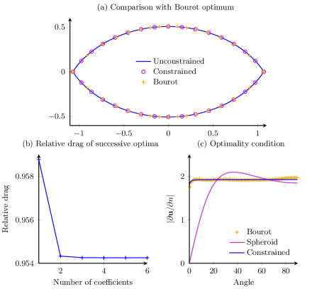
Figure 2: (a): The lowest drag shape of fixed volume as calculated by constrained (fixed front/rear angle) and unconstrained optimisation, together with the shape originally given by Bourot (1974); (b): The drag relative to a sphere of unit volume of succesive optima in found by our constrained optimisation and (c): Pironneau’s optimality condition over the surface of Bourot’s optimum, the optimal prolate spheroid of fixed volume and our constrained optimum.

As a second numerical check, we verify that expanding the tangent angle in terms of Legendre modes provides an efficient description of the lowest drag shape of fixed volume. We consider both an optimisation scheme whereby the front and rear semi-cone angles are constrained to $60^{\circ}$ (see above), and a fully unconstrained optimisation. Figure 2a shows our constrained and unconstrained optima for $6$ Legendre modes in comparison to the shape given by Bourot (1974), described by $10$ coefficients of the equation

$$\frac{r(\theta)}{\lambda}=2-\frac{2}{\sqrt{3}}\sin\theta+\sum_{n=1}^{10}B_{n}\sin^{n+1}\theta.$$ (26)

The values for the coefficients given by Bourot (1974) are truncated to $4$ s.f., and their shape does not quite have the same volume as a sphere of unit radius. Nonetheless, it is clear that our description of the tangent angle by odd Legendre modes yields the optimal shape quickly, see e.g. the convergence of the relative drag in figure 2b. This fast convergence is why a large number of elements ($N=800$) are required in the unconstrained optimisation for the angle at the tip to converge to $60^{\circ}$. Note that the optimal shape for only $3$ Legendre modes is almost indiscernible from our final optimal. After $6$ modes in the unconstrained optimisation, the calculated tip angle converged with $2\%$ relative error. The relative drag of the optimal shape (ratio of drag to that of sphere of equivalent volume) is $D_{r}=0.9542549$, in agreement with the result of Bourot, $D_{r}=0.95425$. Pironneau’s optimality condition of a constant surface vorticity is also confirmed to be valid in figure 2c.

In order to provide a base-line comparison for the numerical shapes, the drag was first minimised for among the family of prolate spheroids of varying eccentricity for both fixed volume and fixed surface area using the analytical result in equation (25) and our boundary element code. The computational code achieves results identical to within $10^{-8}$ of the analytical ones and the optimal spheroids have eccentricities $e=0.8588$ (aspect ratio 1.952) in the fixed-volume case and $0.9688$ (aspect ratio 4.037) in the fixed-surface-area case. We show these results in figure 3, and they allow us to anticipate on two key facts of drag minimisation for fixed surface areas. First, we can predict that the lowest drag shape of fixed surface area is likely to be more slender than its fixed-volume counterpart (this was already anticipated in the local analysis above). Furthermore, we can expect that the reduction in drag of the fixed-surface-area optimum relative to its equivalent sphere will be greater than the fixed volume counterpart; indeed, for spheroids, the reduction in drag is $11\%$ for fixed surface area but only $4.45\%$ for fixed volume.

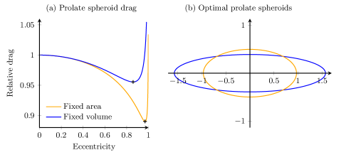
Figure 3: (a): The drag on prolate spheroids of fixed volume (dark blue) and surface area (light yellow) relative to their equivalent spheres as a function of eccentricity. The minimum drag prolate spheroids are marked with plusses; (b): Shape of the minimum drag prolate spheroids of fixed volume and surface area, normalised to unit volume.

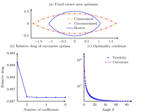
Figure 4: (a): The lowest drag shape of fixed surface as calculated by unconstrained ($+$) and constrained optimisation (i.e. fixed tip angles, light yellow line), in comparison with the fixed volume case (dark blue line). Both shapes are normalized to have unit volume; (b): The drag relative to a sphere of unit surface area for successive optima using constrained optimisation; (c): Vorticity ($+$) along the surface of the optimal shape of fixed surface area shown with its mean curvature, scaled by the ratio of vorticity to curvature at $\theta=90^{\circ}$ (solid purple line).

We now compute the fixed-surface-area analogue of Pironneau’s shape using both unconstrained and constrained (i.e. fixed tip angle) optimisation. After $6$ modes in the unconstrained optimisation, the calculated tip angle converged to the analytically calculated optimal of $30.8^{\circ}$ (equation 18) with a $1\%$ relative error. The optimal shape found with both optimisation approaches is displayed in figure 4a. The unconstrained and constrained results are indistinguishable. We also included in figure 4a the fixed-volume optimal, with all shape volumes normalised to $1$ in order to facilitate comparison. As anticipated, the fixed-area optimal is much more slender than the best shape of fixed volume (aspect ratio of $4.162$ against $2.109$, which are both slightly above the aspect ratios of the optimal spheroids). As with the volume constraint, the drag converges here to its optimal value with very few modes, which is illustrated in figure 4b. The first six unconstrained coefficients describing the tangent angle in equation (23) are

$$A_{1}= -0.47956, A_{2}= -0.035208, A_{3}= -0.0096958,$$

$$A_{4}= -0.0042400, A_{5}= -0.0022198, A_{6}= -0.0012228.$$ (27)

How much better than the equivalent sphere is the optimal shape? The drag ratio we obtain is equal to $D_{r}=0.8871581$, so a drag reduction of about 11.3%. This is significantly greater than the $4.57\%$ reduction for the case of fixed volume. Finally we are able to test numerically the optimality criterion derived in equation (11). We plot in 4c both the value of the flow vorticity on the surface and the mean surface curvature, $\kappa$. As can be seen, our computational results show a perfect proportionally between both, confirming the validity of the local analytical criterion discussed in Sec. 2.1.

4 Conclusion

Shape optimisation at small scales is of potential significance for problems in chemistry and colloidal science. In this work, we used the boundary element method together with a mathematical analysis to determine computationally the convex, axisymmetric shape that minimises drag in Stokes flow subject to the constraint of a fixed surface area. The shape is about twice as slender as the fixed volume case, and the front and rear ends of the shape are tangent to a cone of semi-angle $\approx 30.8^{\circ}$. This was borne out by minimisation of the drag with respect to coefficients of an efficient representation of the shape’s tangent angle in terms of Legendre modes. Although we did not mathematically prove that the shape we obtained is globally optimal, or in fact unique, among all axisymmetric convex ones, since it quickly converges to it from all initial conditions, we conjecture that it is.

From a practical standpoint, while the optimality conditions for the fixed volume and surface area shapes entail the vorticity on the surface of these shapes, the drag turns out to be somewhat insensitive to details of surface vorticity. In fact, the optimal prolate spheroids of fixed volume and surface area both have zero vorticity at the front and rear ends, but only exhibit $0.1\%$ and $0.3\%$ more drag than their respective full optima. This insensitivity engenders the notion of “nearly optimal design” in Stokes flow; optimisation of simple shapes can be effective and helpful to experimental design.

Acknowledgements

This work was funded in part by a European Union Marie Curie CIG to EL and a Royal Commission for the Exhibition of 1851 Research Fellowship to TDMJ.

References

- Alonso et al. (2009) Alonso, J.J., LeGresley, P. & Pereyra, V. 2009 Aircraft design optimization. Math. Comput. Simul. 79 (6), 1948–1958.
- Bourot (1974) Bourot, J-M. 1974 On the numerical computation of the optimum profile in stokes flow. Journal of Fluid Mechanics 65 (03), 513–515.
- Campana et al. (2009) Campana, E.F., Liuzzi, G., Lucidi, S., Peri, D., Piccialli, V. & Pinto, A. 2009 New global optimization methods for ship design problems. Optim. Eng. 10 (4), 533–555.
- Champion et al. (2007) Champion, J.A., Katare, Y.K. & Mitragotri, S. 2007 Particle shape: a new design parameter for micro-and nanoscale drug delivery carriers. J. Cont. Rel. 121 (1), 3–9.
- Champion & Mitragotri (2006) Champion, J.A. & Mitragotri, S. 2006 Role of target geometry in phagocytosis. Proc. Nat. Acad. Sci. 103 (13), 4930–4934.
- Chwang & Wu (1975) Chwang, A.T. & Wu, T. 1975 Hydromechanics of low-Reynolds-number flow. Part 2. Singularity method for Stokes flows. Journal of Fluid Mechanics 67 (04), 787–815.
- Eloy & Lauga (2012) Eloy, C. & Lauga, E. 2012 Kinematics of the most efficient cilium. Phys. Rev. Lett. 109, 038101.
- Gratton et al. (2008) Gratton, S.E.A., Ropp, P.A., Pohlhaus, P.D., Luft, J.C., Madden, V.J., Napier, M.E. & DeSimone, J.M. 2008 The effect of particle design on cellular internalization pathways. Proc. Nat. Acad. Sci. 105 (33), 11613–11618.
- Jameson et al. (1998) Jameson, A., Martinelli, L. & Pierce, N.A. 1998 Optimum aerodynamic design using the navier–stokes equations. Theoret. Comp. Fluid Dyn. 10 (1-4), 213–237.
- Keaveny et al. (2013) Keaveny, E. E., Walker, S. W. & Shelley, M. J. 2013 Optimization of chiral structures for microscale propulsion. Nano lett 13 (2), 531–537.
- Lauga & Eloy (2013) Lauga, E. & Eloy, C. 2013 Shape of optimal active flagella. J. Fluid Mech. 730, R1.
- Mitragotri & Lahann (2009) Mitragotri, S. & Lahann, J. 2009 Physical approaches to biomaterial design. Nat. mat. 8 (1), 15–23.
- Mohammadi & Pironneau (2004) Mohammadi, B. & Pironneau, O. 2004 Shape optimization in fluid mechanics. Annu. Rev. Fluid Mech. 36, 255–279.
- Monteiller et al. (2007) Monteiller, C., Tran, L., MacNee, W., Faux, S., Jones, A., Miller, B. & Donaldson, K. 2007 The pro-inflammatory effects of low-toxicity low-solubility particles, nanoparticles and fine particles, on epithelial cells in vitro: the role of surface area. Occupat. Enviro. Med. 64 (9), 609–615.
- Osterman & Vilfan (2011) Osterman, N & Vilfan, A. 2011 Finding the ciliary beating pattern with optimal efficiency. Proc. Nat. Acad. Sci. 108 (38), 15727–15732.
- Petros & DeSimone (2010) Petros, R.A. & DeSimone, J.M. 2010 Strategies in the design of nanoparticles for therapeutic applications. Nat. Rev. Drug Disc. 9 (8), 615–627.
- Pironneau (1973) Pironneau, O. 1973 On optimum profiles in Stokes flow. J. Fluid Mech. 59 (01), 117–128.
- Pironneau & Katz (1974) Pironneau, O. & Katz, D. F. 1974 Optimal swimming of flagellated micro-organisms. J. Fluid Mech. 66 (02), 391–415.
- Pozrikidis (1992) Pozrikidis, C. 1992 Boundary Integral and Singularity Methods for Linearized Viscous Flow. Cambridge Univ. Press.
- Pozrikidis (2002) Pozrikidis, C. 2002 A Practical Guide to Boundary Element Methods with the Software Library BEMLIB. Taylor & Francis.
- Roper et al. (2008) Roper, M., Pepper, R.E., Brenner, M.P. & Pringle, A. 2008 Explosively launched spores of ascomycete fungi have drag-minimizing shapes. Proc. Nat. Acad. Sci 105 (52), 20583–20588.
- Vilfan (2012) Vilfan, A. 2012 Optimal Shapes of Surface Slip Driven Self-Propelled Microswimmers. Phys. Rev. Lett. 109, 128105.
- Wakiya (1976) Wakiya, S. 1976 Axisymmetric flow of a viscous fluid near the vertex of a body. J. Fluid Mech. 78 (04), 737–747.
- Zabarankin (2013) Zabarankin, M. 2013 Minimum-resistance shapes in linear continuum mechanics. Proc. Roy. Soc. A 469 (2160), 20130206.