Entropy stable wall boundary conditions for the three-dimensional compressible Navier–Stokes equations

Abstract

Non-linear entropy stability and a summation-by-parts framework are used to derive entropy stable wall boundary conditions for the three-dimensional compressible Navier–Stokes equations. A semi-discrete entropy estimate for the entire domain is achieved when the new boundary conditions are coupled with an entropy stable discrete interior operator. The data at the boundary are weakly imposed using a penalty flux approach and a simultaneous-approximation-term penalty technique. Although discontinuous spectral collocation operators on unstructured grids are used herein for the purpose of demonstrating their robustness and efficacy, the new boundary conditions are compatible with any diagonal norm summation-by-parts spatial operator, including finite element, finite difference, finite volume, discontinuous Galerkin, and flux reconstruction/correction procedure via reconstruction schemes. The proposed boundary treatment is tested for three-dimensional subsonic and supersonic flows. The numerical computations corroborate the non-linear stability (entropy stability) and accuracy of the boundary conditions.

1 Introduction

During the last twenty years, scientific computation has become a broadly-used technology in all fields of science and engineering due to a million-fold increase in computational power and the development of advanced algorithms. However, the great frontier is in the challenge posed by high-fidelity simulations of real-world systems, that is, in truly transforming computational science into a fully predictive science. Much of scientific computation’s potential remains unexploited–in areas such as engineering design, energy assurance, material science, Earth science, medicine, biology, security and fundamental science–because the scientific challenges are far too gigantic and complex for the current state-of-the-art computational resources [1].

In the near future, the transition from petascale to exascale systems will provide an unprecedented opportunity to attack these global challenges using modeling and simulation. However, exascale programming models will require a revolutionary approach, rather than the incremental approach of previous projects. Rapidly changing high performance computing (HPC) architectures, which often include multiple levels of parallelism through heterogeneous architectures, will require new paradigms to exploit their full potential. However, the complexity and diversity of issues in most of the science community are such that increases in computational power alone will not be enough to reach the required goals, and new algorithms, solvers and physical models with better mathematical and numerical properties must continue to be developed and integrated into new generation supercomputer systems.

In computational fluid dynamics (CFD), next generation numerical algorithms for use in large eddy simulations (LES) and hybrid Reynolds-averaged Navier–Stokes (RANS)-LES simulations will undoubtedly rely on efficient high-order accurate formulations (see, for instance, [2, 3, 4, 5, 6, 7, 8, 9, 10, 11, 12, 13, 14, 15]). Although high order techniques are well suited for smooth solutions, numerical instabilities may occur if the flow contains discontinuities or under-resolved physical features. A variety of mathematical stabilization strategies are commonly used to cope with this problem (e.g., filtering [16], weighted essentially non-oscillatory (WENO) [17], artificial dissipation, and limiters[2]), but their use for practical complex flow applications in realistic geometries is still problematic.

A very promising and mathematically rigorous alternative is to focus directly on discrete operators that are non-linearly stable (entropy stable) for the Navier–Stokes equations. These operators simultaneously conserve mass, momentum, energy, and enforce a secondary entropy constraint. This strategy begins by identifying a non-linear neutrally stable flux for the Euler equations. An appropriate amount of dissipation can then be added to achieve the desired smoothness of the solution. Regardless of whether dissipation is added, enforcing a semi-discrete entropy constraint enhances the stability of the base operator.

The idea of enforcing entropy stability in numerical operators is quite old [18], and is commonly used for low-order operators [19, 20]. An extension of these techniques to include high-order accurate operators recently appears in references [21, 22, 23, 24] and provides a general procedure for developing entropy conservative and entropy stable, diagonal norm summation-by-parts (SBP) operators for the compressible Navier–Stokes equations. The strong conservation form representation allows them to be readily extended to capture shocks via a comparison approach [19, 22]. The generalization to multi-domain operators follows immediately using simultaneous-approximation-term (SAT) penalty type interface conditions [25], whereas the extension to three-dimensional (3D) curvilinear coordinates is obtained by using an appropriate coordinate transformation which satisfies the discrete geometric conservation law [26]. See reference LeFloch and Rohde [27] for a more comprehensive discussion on high order schemes and entropy inequalities. Therein, the focus is on the approximation of under-compressive, regularization-sensitive, non-classical solutions of hyperbolic systems of conservation laws by high-order accurate, conservative, and semi-discrete finite difference methods.

Several major hurdles remain, however, on the path towards complete entropy stability of the compressible Navier–Stokes equations including shocks. A major obstacle is the need for solid wall viscous boundary conditions that preserve the entropy stability property of the interior operator. In fact, practical experience indicates that numerical instability frequently originates at solid walls, and the interaction of shocks with these physical boundaries is particularly challenging for high order formulations. An important step towards entropy stable boundary conditions appears in the work of Svärd and Özcan [28]. Therein, entropy stable boundary conditions for the compressible Euler equations are reported for the far-field and for the Euler no-penetration wall conditions, in the context of finite difference approximations.

The focus herein is on building non-linearly stable wall boundary conditions for the compressible Navier–Stokes equations; primarily a task of developing stable wall boundary conditions for the viscous terms. At the semi-discrete level, the proposed boundary treatment mimics exactly the boundary contribution obtained by applying the entropy stability analysis to the continuous, compressible Navier–Stokes equations. Furthermore, the new technique enforces the Euler no-penetration wall condition as well as the remaining no-slip and thermal wall conditions in a weak sense. The thermal boundary condition is imposed by prescribing the heat entropy flow (or heat entropy transfer), which is the primary means for exchanging entropy between two thermodynamic systems connected by a solid viscous wall. Note that the entropy flow at a wall is a quantity that in some experiments is directly or indirectly available (e.g., through measurements of the wall heat flux and temperature in some supersonic or hypersonic wind tunnel experiments), or can be estimated from geometrical parameters and fluid flow conditions for the problem at hand. For fluid-structure interaction simulations, (e.g., supersonic and hypersonic flow past aerospace vehicles, heat-exchangers), the entropy flow can be numerically computed at no additional cost while numerically solving the coupled systems of partial differential equations of the continuum mechanics and fluid dynamics.

Historically, most boundary condition analysis for the Navier–Stokes equations is performed at the linear level by linearizing about a known state; a rich collection of literature is available [29, 30, 31, 32]. The non-linear wall boundary conditions developed herein are fundamentally different from those derived using linear analysis and cannot rely on a complete mathematical theory. In fact, a fundamental shortcoming that limits further development of any entropy stable boundary conditions is the incomplete development of the analysis at the continuous level for proving well-posedness of the compressible Navier–Stokes equations. Nevertheless, the boundary conditions proposed herein is extremely powerful because they provide a mechanism for ensuring the non-linear stability in the $L^{2}$ norm of the semi-discretized compressible Navier–Stokes equations. In fact, they allow for a priori bounds on the entropy function when imposing “solid viscous wall” boundary conditions. The new boundary conditions are easy to implement and compatible with any diagonal norm SBP spatial operator, including finite element (FE), finite volume (FV), finite difference (FD) schemes and the more recent class of high-order accurate methods which include the large family of discontinuous Galerkin (DG) discretizations [33] and flux reconstruction (FR) schemes [34].

The robustness and accuracy of the complete semi-discrete operator (i.e., the entropy stable interior operator coupled with the new boundary conditions) is demonstrated by computing subsonic and supersonic flows past a 3D square cylinder without any stabilization technique (e.g., artificial dissipation, filtering, limiters, de-aliasing, etc.), a feat unattainable with several alternative approaches to wall boundary conditions based on linear analysis. In fact, instabilities are observed when wall boundary conditions designed with linear analysis are used in combination with highly clustered grids and/or high order polynomials, or very coarse grids near solid walls, which yield unresolved physical flow features.

The paper is organized as follows. In Section 2, the compressible Navier–Stokes equations, their entropy function and symmetrized form are introduced. Section 3 presents the entropy analysis of the viscous wall boundary conditions at the continuous level. Section 4 provides a discussion of the inviscid flux condition which allows the construction of high-order accurate entropy conservative and entropy stable fluxes at the semi-discrete level, for the interior operator. The new entropy stable wall boundary conditions and their non-linear stability (entropy stability) analysis are presented in Section 5. Finally, the accuracy and high level robustness of the proposed approach in combination with a discontinuous high-order accurate entropy stable interior operator are demonstrated in Section 6. Conclusions are discussed in Section 7.

2 The compressible Navier–Stokes equations

Consider a fluid in a domain $\Omega$ with boundary surface denoted by $\partial\Omega$, without radiation and external volume forces. In this context, the compressible Navier–Stokes equations, equipped with suitable boundary and initial conditions, may be expressed in the form

$$\frac{\partial q}{\partial t}+\frac{\partial f^{(I)}_{i}}{\partial x_{i}}=\frac{\partial f^{(V)}_{i}}{\partial x_{i}},\quad x\in\Omega,\quad t\in[0,\infty),$$ (1)

$$q|_{\partial\Omega}=g^{(B)}(x,t),\quad x\in\partial\Omega,\quad t\in[0,\infty),$$

$$q(x,0)=g^{(0)}(x),\quad x\in\Omega,$$

where the Cartesian coordinates, $x=\left(x_{1},x_{2},x_{3}\right)^{\top}$, and time, $t$, are the independent variables. Note that in (1) Einstein notation is used. The vectors $q(x,t)$, $f^{(I)}_{i}=f^{(I)}_{i}(q)$, and $f^{(V)}_{i}=f^{(V)}_{i}(q,\nabla q)$ are the conserved variables, and the inviscid and viscous fluxes in the $i$ direction, respectively. Both boundary data, $g^{(B)}$, and initial data, $g^{(0)}$, are assumed to be bounded, $L^{2}\cap L^{\infty}$. Furthermore, $g^{(B)}$ is also assumed to contain (linearly) well-posed Dirichlet and/or Neumann and/or Robin data. The vector of the conservative variables is

$$q=\left(\rho,\rho u_{1},\rho u_{2},\rho u_{3},\rho E\right)^{\top},$$ (2)

where $\rho$ denotes the density, $u=\left(u_{1},u_{2},u_{3}\right)^{\top}$ is the velocity vector, and $E$ is the specific total energy, which is the sum of the specific internal energy, $e$, (defined later) and the kinetic energy, $\frac{1}{2}u_{j}u_{j}$. The convective fluxes are

$$f^{(I)}_{i}=\left(\rho u_{i},\rho u_{i}u_{1}+\delta_{i1}p,\rho u_{i}u_{2}+\delta_{i2}p,\rho u_{i}u_{3}+\delta_{i3}p,\rho u_{i}H\right)^{\top},$$ (3)

where $p$, $H$ and $\delta_{ij}$ are the pressure, the specific total enthalpy and the Kronecker delta, respectively. The viscous fluxes are

$$f^{(V)}_{i}=\left(0,\tau_{i1},\tau_{i2},\tau_{i3},\tau_{ji}u_{j}-\mathtt{q}_{i}\right)^{\top},$$ (4)

where the shear stress tensor, $\tau_{ij}$, assuming a zero bulk viscosity, is defined as

$$\tau_{ij}=\mu\left(\frac{\partial u_{i}}{\partial x_{j}}+\frac{\partial u_{j}}{\partial x_{i}}-\delta_{ij}\,\frac{2}{3}\frac{\partial u_{k}}{\partial x_{k}}\right),$$ (5)

and the heat flux, according to the Fourier heat conduction law, is

$$\mathtt{q}_{i}=-\kappa\,\frac{\partial T}{\partial x_{i}}.$$ (6)

The symbols $T$, $\mu=\mu\left(T\right)$ and $\kappa=\kappa\left(T\right)$ which appear in (5) and (6) denote the temperature, the dynamic viscosity and the thermal conductivity, respectively. The viscous fluxes in (4) can also be expressed as

$$f^{(V)}_{i}=c_{ij}\,\frac{\partial q}{\partial x_{j}}=c_{ij}^{\prime}\frac{\partial v}{\partial x_{j}},$$ (7)

where $c_{ij}$ and $c_{ij}^{\prime}$ are variable five-by-five matrices and $v=\left(\rho,u_{1},u_{2},u_{3},T\right)^{\top}$ is the vector of the primitive variables. The functional form of the matrices $c_{ij}^{\prime}$ is given in A. As we will show later, relation (7) is a very convenient form for the entropy stability analysis.

The constitutive relations for a calorically perfect gas are

$$e=c_{v}\,T,\quad h=H-\frac{1}{2}u_{j}\,u_{j}=c_{p}\,T,$$ (8)

where the symbols $c_{v}$ and $c_{p}$ denote the specific heat capacity at constant volume and constant pressure, respectively, and

$$p=\rho R\,T,\quad R=\frac{R_{u}}{MW},$$ (9)

where $R_{u}$ is the universal gas constant and $MW$ is the molecular weight of the gas. The speed of sound for a perfect gas is

$$c=\sqrt{\gamma R\,T},\quad\gamma=\frac{c_{p}}{c_{p}-R}.$$ (10)

In the entropy analysis that will follow, the definition of the thermodynamic entropy is the explicit form,

$$s=\frac{R}{\gamma-1}\log\left(\frac{T}{T_{\infty}}\right)-R\log\left(\frac{\rho}{\rho_{\infty}}\right),$$ (11)

where $T_{\infty}$ and $\rho_{\infty}$ are the reference temperature and density, respectively.

Note that in practical situations, most simulations are performed in computational space, that is, by transforming all grid elements in physical space to standard elements in computational space via a smooth mapping. However, to keep the notation as simple as possible, a uniform Cartesian grid is considered in the derivations presented herein. The extension to generalized curvilinear coordinates and unstructured grids follows immediately if the transformation from computational to physical space preserves the semi-discrete geometric conservation (GCL) [26].

2.1 Entropy function and entropy variables of the compressible Navier–Stokes equations

In the linear hyperbolic framework, $L^{2}$ stability is sought as a discrete analogue for a priori energy estimates available in the differential formulation (e.g., Richtmyer and Morton [35] and Gustafsson, Kreiss and Oliger [29]; Kreiss and Lorenz [36]). In the context of non-linear problems dominated by non-linear convection, we seek entropy stability as a discrete analogue for the corresponding statement in the differential formulation [19]. Moreover, for systems of conservation laws, stability with respect to a mathematical entropy function is considered as an admissibility criterion for selecting physically relevant weak solutions. In fact, the entropy condition plays a decisive role in the theory and numerics of such problems as shown, for instance, by Lax [37] and Smoller [38].

Harten [39] and Tadmor [40] showed that systems of conservation laws are symmetrizable if and only if they are equipped with a convex mathematical entropy function. Given a set of conservation variables $q(x,t)$, the entropy variables which symmetrize the system are defined as the derivatives of the mathematical entropy function with respect to $q(x,t)$. Hughes and co-authors [18] extended these ideas to the compressible Navier–Stokes equations (1). Therein, it is shown that the mathematical entropy must be an affine function of the physical (or thermodynamic) entropy function and that semi-discrete solutions obtained from a weighted residual formulation based on entropy variables will respect the second law of thermodynamics. Hence, it is again found that the entropy function and the entropy variables are critical ingredients in the design of numerical schemes exhibiting non-linear stability.

Definition 2.1.

A scalar function $S=S(q)$ is an entropy function of Equation (1) if it satisfies the following conditions:

• The function $S(q)$ when differentiated with respect to the conservative variables (i.e., $\partial S/\partial q$) simultaneously contracts all the inviscid spatial fluxes as follows

  $$\frac{\partial S}{\partial q}\,\frac{\partial f^{(I)}_{i}}{\partial x_{i}}\>=\>\frac{\partial S}{\partial q}\frac{\partial f^{(I)}_{i}}{\partial q}\,\frac{\partial q}{\partial x_{i}}\>=\>\frac{\partial F_{i}}{\partial q}\,\frac{\partial q}{\partial x_{i}}\>=\>\frac{\partial F_{i}}{\partial x_{i}},\quad i=1,2,3.$$ (12)

  The components of the contracting vector, $\partial S/\partial q$, are the entropy variables denoted as $w^{\top}\>=\>\partial S/\partial q$. $F_{i}(q),\,i=1,2,3,$ are the entropy fluxes in the three Cartesian directions.

• The new entropy variables, $w$, symmetrize Equation (1):

  $$\frac{\partial q}{\partial t}+\frac{\partial f^{(I)}_{i}}{\partial x_{i}}-\frac{\partial f^{(V)}_{i}}{\partial x_{i}}\>=\>\frac{\partial q}{\partial w}\,\frac{\partial w}{\partial t}+\frac{\partial f^{(I)}_{i}}{\partial w}\,\frac{\partial w}{\partial x_{i}}-\frac{\partial}{\partial x_{i}}\left(\widehat{c}_{ij}\,\frac{\partial w}{\partial x_{j}}\right)=0,\quad i=1,2,3$$ (13)

  with the symmetry conditions: $\partial q/\partial w=\left(\partial q/\partial w\right)^{\top}$, $\partial f^{(I)}_{i}/\partial w=\left(\partial f^{(I)}_{i}/\partial w\right)^{\top}$ and $\widehat{c}_{ij}={\widehat{c}_{ij}}^{\top}$, with the matrices $\,\widehat{c}_{ij}$ included in A.

The mathematical entropy is convex, meaning that the Hessian, $\partial^{2}S/\partial q^{2}\>=\>\partial w/\partial q$, is symmetric positive definite (SPD),

$$\quad\zeta^{T}\,\frac{\partial^{2}S}{\partial q^{2}}\,\zeta>0,\quad\forall\zeta\neq 0,$$ (14)

and yields a one-to-one mapping from conservation variables, $q$, to entropy variables, $w^{\top}\>=\>\partial S/\partial q$. Likewise, $\partial w/\partial q$ is SPD because $\partial q/\partial w=\left({\partial w/\partial q}\right)^{-1}$ and SPD matrices are invertible. The entropy and corresponding entropy flux are often denoted as entropy–entropy flux pair, $(S,F)$, [19]. If the entropy function $S(q)$ is convex, a bound on its global estimate can be converted into an a priori estimate on the solution of (1) in suitable $L^{p}$ space [41].

The symmetry of the matrices $\partial q/\partial w$, $\partial f^{(I)}_{i}/\partial w$ indicates that the conservative variables, $q$, and the inviscid fluxes, $f^{(I)}_{i}$, are Jacobians of scalar functions with respect to the entropy variables,

$$q^{\top}=\frac{\partial\varphi}{\partial w},\quad\left(f^{(I)}_{i}\right)^{\top}=\frac{\partial\psi_{i}}{\partial w},$$ (15)

where the non-linear function $\varphi$ is called the potential and $\psi_{i},\,i=1,2,3$, are called the potential fluxes [19]. Just as the entropy function is convex with respect to the conservative variables ($\partial^{2}S/\partial q^{2}$ is SPD), the potential function is convex with respect to the entropy variables.

Godunov [42] proved that (see reference [39] for a detailed summary of the proof):

Theorem 2.1.

If Equation (1) can be symmetrized by introducing new variables $w$, and $q$ is a convex function of $\varphi$ (the so-called potential), then an entropy function $S(q)$ is given by

$$\varphi=w^{\top}q-S,$$ (16)

and the entropy fluxes satisfy

$$\psi_{i}=w^{\top}f^{(I)}_{i}-F_{i},$$ (17)

where $\psi_{i},i=1,2,3,$, are the so-called potential fluxes. The potential and the corresponding potential flux are usually denoted as potential–potential flux pair, $(\varphi,\psi)$, [19].

In the specific case of the compressible Navier–Stokes equations, the entropy–entropy flux pair is

$$S=-\rho\,s,\quad F_{i}=-\rho\,u_{i}\,s,\quad i=1,2,3,$$ (18)

and the potential–potential flux pair is

$$\varphi=\rho\,R,\quad\psi_{i}=\rho\,u_{i}\,R,\quad i=1,2,3.$$ (19)

Note that the mathematical entropy has the opposite sign of the thermodynamic entropy. To avoid confusion, herein entropy refers to the mathematical entropy unless otherwise noted. The entropy variables using the pair in (18) result in

$$w=\left(\frac{\partial S}{\partial q}\right)^{\top}=\left(\frac{h}{T}-s-\frac{u_{i}u_{i}}{2T},\frac{u_{1}}{T},\frac{u_{2}}{T},\frac{u_{3}}{T},-\frac{1}{T}\right)^{\top}.$$ (20)

A sufficient condition to ensure the convexity of the entropy function $S(q)$ (and, hence, a one-to-one mapping between the entropy variables (20) and the conservative variables (2)) is that $\rho,T>0$ (for the proof see, for instance, Appendix B.1 in [22]). Expressly:

$$\zeta^{T}\,\frac{\partial^{2}S}{\partial q^{2}}\,\zeta^{T}>0,\quad\forall\zeta\neq 0,\quad\rho,T>0.$$

This restriction on density and temperature weakens the entropy proof, making it less than full measure of non-linear stability. Another mechanism must be employed to bound $\rho$ and $T$ away from zero to guarantee stability and positivity; positivity preservation will not be considered herein.

Remark 2.1.

The semi-discrete entropy stability does not necessarily lead to fully discrete stability as is usually the case for linear partial differential equations (PDEs). However, as noted by Tadmor [19], entropy stability is enhanced by fully implicit time discretization. For example, the fully implicit backward Euler time discretization is unconditionally entropy-stable and is responsible for additional entropy dissipation. In contrast, explicit time discretization, leads to entropy production. Thus, the entropy stability of explicit schemes hinges on a delicate balance between temporal entropy production and spatial entropy dissipation. For example, the fully explicit Euler time discretization does not conserve entropy except in the case of linear fluxes [27]. Consequently, both the fully explicit and fully implicit Euler differencing do not respect (non-linear) entropy conservation, independent of the spatial discretization. Fully discrete entropy conservation is offered, for instance, by Crank–Nicolson time differencing [19].

3 No-slip boundary conditions: Continuous analysis

The problem of well-posed boundary conditions is an essential question in many area of physics. For the two- (2D) and three-dimensional (3D) Navier–Stokes equations, the number of boundary conditions implying well-posedness can be obtained using the Laplace transform technique [29]; a complicated procedure for system of PDEs like the compressible Navier–Stokes equations. Nordström and Svärd [30] proposed an alternative semi-discrete approach to arrive at the number and type of boundary conditions for a general time-dependent system of PDEs. This analysis was applied to the 3D compressible Navier–Stokes equations for different flow regimes and the case of the Euler no-penetration velocity condition.

In 2008, Svärd and Nordström [31] showed that the no-slip boundary conditions together with a boundary condition on the temperature imply stability for the linearized compressible Navier–Stokes equations. Their result, can also be generalized to assess the stability of the non-linear problem for smooth solutions as indicated in [43, 29] and references therein. In 2011, Berg and Nordström [32] proved that the no-slip boundary conditions together with a thermal Robin boundary condition also imply stability for the same linearized equations. In this section we address the non-linear stability (entropy stability) of the wall boundary conditions for the (non-linear) compressible Navier–Stokes equations given in (1). The aim is to derive a sharp a priori bound for the entropy function which holds for smooth and non-smooth solutions.

Contracting the system of equations (1) with the entropy variables and using the relations given in (12) and (13) results in the differential form of the (scalar) entropy equation:

$$\frac{\partial S}{\partial q}\frac{\partial q}{\partial t}+\frac{\partial S}{\partial q}\frac{\partial f^{(I)}_{i}}{\partial x_{i}}=\frac{\partial S}{\partial t}+\frac{\partial F_{i}}{\partial x_{i}}=\frac{\partial S}{\partial q}\frac{\partial f^{(V)}_{i}}{\partial x_{i}} =\frac{\partial}{\partial x_{i}}\left(w^{\top}f^{(V)}_{i}\right)-\left(\frac{\partial w}{\partial x_{i}}\right)^{\top}f^{(V)}_{i}$$ (21)

$$=\frac{\partial}{\partial x_{i}}\left(w^{\top}f^{(V)}_{i}\right)-\left(\frac{\partial w}{\partial x_{i}}\right)^{\top}\widehat{c}_{ij}\,\frac{\partial w}{\partial x_{j}}.$$

Integrating Equation (21) over the domain yields a global conservation statement for the entropy in the domain,

$$\frac{d}{dt}\int_{\Omega}S\,\mathrm{d}{{\mathbf{x}}}\>=\>\left[w^{\top}f^{(V)}_{i}-F_{i}\right]_{\partial\Omega}-\int_{\Omega}\left(\frac{\partial w}{\partial x_{i}}\right)^{\top}\widehat{c}_{ij}\,\frac{\partial w}{\partial x_{j}}\,\,\mathrm{d}{{\bf x}}\>=\>\left[w^{\top}f^{(V)}_{i}-F_{i}\right]_{\partial\Omega}\>-\>DT,$$ (22)

where $DT$ is the viscous dissipation term,

$$DT=\mathop{\text{\Large$\int_{\text{\normalsize$\scriptstyle\Omega$}}$}}\nolimits\left(\frac{\partial w}{\partial x_{i}}\right)^{\top}\widehat{c}_{ij}\,\frac{\partial w}{\partial x_{j}}\,\,\mathrm{d}{{\bf x}}=\mathop{\text{\Large$\int_{\text{\normalsize$\scriptstyle\Omega$}}$}}\nolimits\begin{pmatrix}\partial w/\partial x_{1}\\ \partial w/\partial x_{2}\\ \partial w/\partial x_{3}\end{pmatrix}^{\top}\begin{pmatrix}\widehat{c}_{11}&\widehat{c}_{12}&\widehat{c}_{13}\\ \widehat{c}_{21}&\widehat{c}_{22}&\widehat{c}_{23}\\ \widehat{c}_{31}&\widehat{c}_{32}&\widehat{c}_{33}\\ \end{pmatrix}\begin{pmatrix}\partial w/\partial x_{1}\\ \partial w/\partial x_{2}\\ \partial w/\partial x_{3}\end{pmatrix}\,\mathrm{d}{{\bf x}}.$$ (23)

This equation indicates that the entropy can only increase in the domain based on data that convects and diffuses through the boundaries. It is shown in [18, 22] that the larger $15\times 15$ coefficient matrix in (23) is positive semi-definite, which makes the term $-DT$ in (22) strictly dissipative. Therefore, the sign of the entropy change due to viscous dissipation is always negative.

To simplify, we let the domain of interest, $\Omega$, be the unit cube $0\leq x_{1},x_{2},x_{3}\leq 1$. Expanding the Einstein notation in equation (22) yields

$$\frac{d}{dt}\int_{\Omega}S\,dx_{1}\,dx_{2}\,dx_{3}=-DT$$ (24)

$$\>+\>\int_{x_{1}=0}\left[+F_{1}-\,w^{\top}\left(\widehat{c}_{11}\frac{\partial w}{\partial x_{1}}+\widehat{c}_{12}\frac{\partial w}{\partial x_{2}}+\widehat{c}_{13}\frac{\partial w}{\partial x_{3}}\right)\right]dx_{2}\,dx_{3}$$

$$\>+\>\int_{x_{1}=1}\left[-F_{1}+\,w^{\top}\left(\widehat{c}_{11}\frac{\partial w}{\partial x_{1}}+\widehat{c}_{12}\frac{\partial w}{\partial x_{2}}+\widehat{c}_{13}\frac{\partial w}{\partial x_{3}}\right)\right]dx_{2}\,dx_{3}$$

$$\>+\>\int_{x_{2}=0}\left[+F_{2}-\,w^{\top}\left(\widehat{c}_{21}\frac{\partial w}{\partial x_{1}}+\widehat{c}_{22}\frac{\partial w}{\partial x_{2}}+\widehat{c}_{23}\frac{\partial w}{\partial x_{3}}\right)\right]dx_{1}\,dx_{3}$$

$$\>+\>\int_{x_{2}=1}\left[-F_{2}+\,w^{\top}\left(\widehat{c}_{21}\frac{\partial w}{\partial x_{1}}+\widehat{c}_{22}\frac{\partial w}{\partial x_{2}}+\widehat{c}_{23}\frac{\partial w}{\partial x_{3}}\right)\right]dx_{1}\,dx_{3}$$

$$\>+\>\int_{x_{3}=0}\left[+F_{3}-\,w^{\top}\left(\widehat{c}_{31}\frac{\partial w}{\partial x_{1}}+\widehat{c}_{32}\frac{\partial w}{\partial x_{2}}+\widehat{c}_{33}\frac{\partial w}{\partial x_{3}}\right)\right]dx_{1}\,dx_{2}$$

$$\>+\>\int_{x_{3}=1}\left[-F_{3}+\,w^{\top}\left(\widehat{c}_{31}\frac{\partial w}{\partial x_{1}}+\widehat{c}_{32}\frac{\partial w}{\partial x_{2}}+\widehat{c}_{33}\frac{\partial w}{\partial x_{3}}\right)\right]dx_{1}\,dx_{2}\,.$$

Consider the case of a wall placed at $x_{1}=0$, and assume that all the other boundaries terms are entropy stable; their contributions are neglected without loosing generality. Therefore, estimate (24) reduces to

$$\frac{d}{dt}\int_{\Omega}S\,dx_{1}\,dx_{2}\,dx_{3}=-DT$$ (25)

$$\>+\>\int_{x_{1}=0}\left[F_{1}-\,w^{\top}\left(\widehat{c}_{11}\frac{\partial w}{\partial x_{1}}+\widehat{c}_{12}\frac{\partial w}{\partial x_{2}}+\widehat{c}_{13}\frac{\partial w}{\partial x_{3}}\right)\right]dx_{2}\,dx_{3}\,.$$

To bound the time derivative of the entropy, the right-hand-side (RHS) of Equation (25) requires boundary data. For a solid viscous wall, assuming linear analysis, four independent boundary conditions must be imposed [43]. Three boundary conditions are the so-called no-slip boundary conditions, $u_{1}=u_{2}=u_{3}=0$ (i.e., the velocity vector relative to the wall is the zero vector). In the linear settings (see, for instance, [32, 31]), the fourth condition is the gradient of the temperature normal to the wall, $(\partial T/\partial n)_{wall}$, (Neumann boundary condition; e.g., the adiabatic wall), or the temperature of the wall, $T_{wall}$, (the Dirichlet or isothermal wall boundary condition), or a mixture of Dirichlet and Neumann conditions (the Robin boundary condition). These four boundary conditions lead to energy stability (linear stability); see, for instance, [31, 32]. In the remainder of this section, we will show the type and the form of the wall boundary conditions that have to be imposed to bound estimate (25) and, hence, to attain entropy stability.

Consider the inviscid contribution to the boundary terms in (25).

Theorem 3.1.

The no-slip boundary conditions $u_{1}=u_{2}=u_{3}=0$ bound the inviscid contribution to the time derivative of the entropy in equation (25).

Proof.

Equation (17) provides the definition of the entropy flux, $F_{1}$:

$$F_{1}=w^{\top}f^{(I)}_{1}-\psi_{1},\quad\psi_{1}=\rho u_{1}R.$$ (26)

Substituting the no-slip conditions, $u_{1}=u_{2}=u_{3}=0$, into the definition of the inviscid flux, $f^{(I)}_{1}$, (Equation 3) and the condition $u_{1}=0$ into the definition of $\psi_{1}$, yields the desired result $F_{1}=0$. ∎

Consider now the viscous contribution to the boundary terms in (25).

Theorem 3.2.

The boundary condition,

$$\mathtt{g}(t)=\frac{\partial T}{\partial n}\frac{1}{T},$$ (27)

where the symbol $n$ defines the normal direction to the wall, bounds the viscous contribution to the time derivative of the entropy (25).

Proof.

Using the definition of matrices $\widehat{c}_{ij}$ given in A, the viscous vector-matrix-vector contraction given in (25) yields the following term

$$-\,w^{\top}\left(\widehat{c}_{11}\frac{\partial w}{\partial x_{1}}+\widehat{c}_{12}\frac{\partial w}{\partial x_{2}}+\widehat{c}_{13}\frac{\partial w}{\partial x_{3}}\right)\>=\>\kappa\left(\frac{\partial T}{\partial x_{1}}\frac{1}{T}\right).$$ (28)

Therefore, specifying the condition $\mathtt{g}(t)=\left(\frac{\partial T}{\partial x_{1}}\frac{1}{T}\right)$ where $\mathtt{g}(t)$ is a known bounded function (i.e., $L^{2}\cap L^{\infty}$), eliminates the last potential source of instability on the right-hand-side of equation (25). ∎

The boundary condition given by Theorem 3.2 at first glance appears ad hoc. Note, however, that the scalar value $\kappa\left(\frac{\partial T}{\partial x_{1}}\frac{1}{T}\right)$ accounts for the change in entropy at the boundary $x_{1}=0$, due to the wall heat flux, $\mathtt{q}_{wall}$, and it is often denoted heat entropy transfer or heat entropy flow [44]. In fact,

$$\kappa\,\frac{\partial T}{\partial x_{1}}\frac{1}{T}=-\kappa\,\frac{\partial}{\partial x_{1}}\left[w(5)\right]\frac{1}{w(5)}=\kappa\,\frac{\partial}{\partial x_{1}}\left[\log(T)\right]=-\frac{\mathtt{q}_{wall}}{T_{wall}},$$ (29)

where $w(5)$ denotes the fifth component of the entropy variable vector, $w$, in (20). Equation (29) indicates that, in the context of the entropy stability analysis of the compressible Navier–Stokes equations, it is admissible and physically (thermodynamically) correct to impose the fourth wall boundary condition as given in Theorem 3.2.

To the best of our knowledge, Theorem 3.2 provides new insight for future development of any entropy stable boundary conditions for the compressible Navier–Stokes equations.

Remark 3.1.

We strongly remark that the non-linear contraction obtained in (28) is different from that obtained from the linearized compressible Navier–Stokes equations [31, 32]. The linear analysis produces velocity gradient terms in the energy estimate (not present in (28)), and temperature gradient terms in the normal direction of the form $T\frac{\partial T}{\partial x_{1}}$, with $T$ and $\frac{\partial T}{\partial x_{1}}$ being perturbations; see, for instance, [31, 32].

Remark 3.2.

The boundary condition $\mathtt{g}(t)=0$, which corresponds to an adiabatic wall $\partial T/\partial x_{1}=0$, bounds the solution, and, as physically expected, does not contribute to the time derivative of the entropy (25) because the heat flux is zero.

4 Entropy stable spectral discontinuous collocation method for the semi-discretized system: Interior operator

In this section, we summarize the main results that allow us to construct a numerical high order entropy stable discontinuous collocation interior operator of any order, $p$, on unstructured grids. The formalism provided here, will then be used in Section 5 to design new entropy stable solid wall boundary conditions for the semi-discretized compressible Navier–Stokes equations.

Using an SBP operator and its equivalent telescoping form (see, for instance, [45, 46]), the semi-discrete form of the compressible Navier–Stokes equations (1) becomes

$$\frac{\partial\mathbf{q}}{\partial t} =\mathcal{D}_{x_{i}}\left(-{\bf f}_{i}^{(I)}+c_{ij}\mathcal{D}_{x_{j}}\mathbf{q}\right)+\mathcal{P}^{-1}_{x_{i}}\left(\mathbf{g}_{i}^{(B)}+\mathbf{g}_{i}^{(In)}\right)$$ (30)

$$=\mathcal{P}^{-1}_{x_{i}}\Delta_{x_{i}}\left(-\mathbf{\overline{f}}^{(I)}_{i}+\mathbf{\overline{f}}_{i}^{(V)}\right)+\mathcal{P}^{-1}_{x_{i}}\left(\mathbf{g}_{i}^{(B)}+\mathbf{g}_{i}^{(In)}\right),$$

$$\mathbf{q}(x,0)=\mathbf{g}^{(0)}(x),\quad x\in\Omega,$$

where the subscript $x_{i}$ indicates the coordinate direction to which the operators apply. The source terms $\mathbf{g}_{i}^{(B)}$ and $\mathbf{g}_{i}^{(In)}$, with $i=1,2,3$, enforce boundary and interface conditions, respectively; and $\mathbf{g}^{(0)}$ represents the initial condition. The matrix $\mathcal{P}$ may be thought of as a mass matrix in the context of Galerkin finite element method. While it is not true in general that $\mathcal{P}$ is diagonal, herein the focus is exclusively on diagonal norm SBP operators, based on fixed element-based polynomials of order $p$. The matrix $\mathcal{D}$ is used to approximate the first derivative; and it is defined as $\mathcal{P}^{-1}\mathcal{Q}$, where the nearly skew-symmetric matrix, $\mathcal{Q}$, is an undivided differencing operator where all rows sum to zero and the first and last column sum to $-1$ and $1$, respectively [45, 46]. The operator $\Delta$ is the telescopic flux matrix and allows to express the semi-discrete system in a telescopic flux form, by evaluating the fluxes at the collocated flux points, $\mathbf{\overline{f}}^{(I)}$ and $\mathbf{\overline{f}}^{(V)}$, (see Figure 1). Note that the spacing between the flux points is incorporated into the operator $\mathcal{P}$. In fact, the diagonal elements of $\mathcal{P}$ are equal to the spacing between flux points. In the remainder of this paper, the elements of $\mathcal{P}$ are denoted as $\mathcal{P}_{(i)(i)},i=1,2,\ldots,N$.

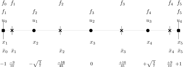
Figure 1: The one-dimensional discretization for $p=4$ Legendre collocation. Solution points are denoted by $\bullet$ and flux points are denoted by $\times$.

The semi-discrete entropy estimate is achieved by mimicking term by term the continuous estimate given in Equation (21). The non-linear analysis (entropy analysis) begins by contracting the semi-discrete equations given in Equation (30) with the entropy variables: $\mathbf{w}^{\top}\mathcal{P}$. For clarity of presentation, but without loss of generality, the derivation is simplified to one spatial dimension. Tensor product algebra allows the results to extend directly to three dimensions. The resulting global equation that governs the time derivative of the entropy is given by

$$\mathbf{w}^{\top}\mathcal{P}\frac{\partial\mathbf{q}}{\partial t}+\mathbf{w}^{\top}\Delta\mathbf{\overline{f}}^{(I)}=\mathbf{w}^{\top}\Delta\mathbf{\overline{f}}^{(V)}+\mathbf{w}^{\top}(\mathbf{g}^{(B)}+\mathbf{g}^{(In)}),$$ (31)

where

$$\mathbf{w}=\left(w(q_{1})^{\top},w(q_{2})^{\top},\dots,w(q_{N})^{\top}\right)^{\top}$$

is the vector of the entropy variables at the solution points.

4.1 Time derivative

The time derivative in (31) is in mimetic form for diagonal norm SBP operators. The entropy variables are defined by the expression $w^{\top}=\partial S/\partial q$ (see Definition 2.1), which when combined with the definition of entropy yields the point-wise expression

$$w_{i}^{\top}\frac{\partial q_{i}}{\partial t}\>=\>\frac{\partial S_{i}}{\partial q_{i}}\frac{\partial q_{i}}{\partial t}\>=\>\frac{\partial S_{i}}{\partial t},\quad\forall i.$$

Now, define the diagonal matrices $\partial{\bf S}/\partial{\bf q}\>=\>\mathbf{W}\>=\>\textrm{diag}[\mathbf{w}]$. Since $\mathcal{P}$ is a diagonal matrix and arbitrary diagonal matrices commute, the semi-discrete rate of change of entropy becomes

$$\mathbf{w}^{\top}\mathcal{P}\frac{\partial\mathbf{q}}{\partial t}\>=\>\mathbf{1}^{\top}\mathbf{W}\mathcal{P}\frac{\partial\mathbf{q}}{\partial t}\>=\>\mathbf{1}^{\top}\mathcal{P}\mathbf{W}\frac{\partial\mathbf{q}}{\partial t}\>=\>\mathbf{1}^{\top}\mathcal{P}\frac{\partial{\bf S}}{\partial\mathbf{q}}\frac{\partial\mathbf{q}}{\partial t}\>=\>\mathbf{1}^{\top}\mathcal{P}\frac{\partial\mathbf{S}}{\partial t},$$

where

$$\mathbf{1}=\left(1,1,\dots,1\right)^{\top}$$

is a vector with $N$ elements.

4.2 Inviscid terms

The inviscid portion of Equation (31) is entropy conservative if it satisfies

$$\mathbf{w}^{\top}\Delta\mathbf{\overline{f}}^{(I)}=\overline{F}(q_{N})-\overline{F}(q_{1})=F(q_{N})-F(q_{1})=\mathbf{1}^{\top}\Delta\mathbf{\overline{F}}.$$ (32)

Note that in (32), the first and last flux points are coincident with the first and last solution points, which enables the endpoint fluxes to be consistent (see Figure 1). Condition (32) leads to globally entropy conservative schemes but it is difficult to enforce at the flux points. One plausible solution to circumvent this problem is to use a more restrictive point-wise relation between solution and flux-point data, which telescopes across the domain and yields a local condition on the flux for the global entropy consistency constraint (32). Tadmor [19] developed such a solution based on second-order accurate centered operators. Carpenter and co-authors [46], have generalized this solution for Legendre spectral collocation operators of any order of accuracy, $p$.

In the following paragraphs, we present, without any proof, the main theorems which allow to construct inviscid entropy conservative and stable fluxes of any order of accuracy, $p$. Interested readers should consult [22, 46] and the references therein for details. Note that in this section the subscripts $i-1$, $i$ and $i+1$ are used to denote a scalar or vector quantity at the $i-1$, $i$ or $i+1$ collocated point, and do not have to be confused with the subscript used, for instance, in (1).

Theorem 4.1.

The local conditions

$$\left(w_{i+1}-w_{i}\right)^{\top}\overline{f}_{i}=\widetilde{\psi}_{i+1}-\widetilde{\psi}_{i},\quad i=1,2,\dots,N-1\quad;\quad\widetilde{\psi}_{1}=\psi_{1},\quad\widetilde{\psi}_{N}=\psi_{N}$$ (33)

when summed, telescope across the domain and satisfy the entropy conservative condition given in Equation (32). A flux that satisfies the condition given in equation (33) is denoted $\bar{f}_{i}^{(S)}$. The potentials $\widetilde{\psi}_{i+1}$ and $\widetilde{\psi}_{i}$ need not be the point-wise ${\psi}_{i+1}$ and ${\psi}_{i}$, respectively.

Proof.

See Theorem 3.3 in reference [46] for the proof of this theorem. ∎

A possible strategy for constructing high order entropy conservative fluxes is to construct a linear combination of two-point entropy conservative fluxes by using the coefficients in the SBP matrix $\mathcal{Q}$. This approach follows immediately from the generalized telescoping structural properties of diagonal norm SBP operators (see, for instance, [45, 46]). Because it requires only the existence of a two-point entropy conservative flux formula and the coefficients of $\mathcal{Q}$, it is valid for any SBP operator that satisfies the following SBP constraints

$$\mathcal{Q}^{\top}=\mathcal{B}-\mathcal{Q},\quad\mathcal{B}=\mathrm{diag}\left(-1,0,\dots,0,1\right).$$

Thus, it is also valid for Legendre spectral collocation operators used herein; see [46].

The following theorem establishes the accuracy of the new fluxes.

Theorem 4.2.

A two-point entropy conservative flux can be extended to high order with formal boundary closures by using the form

$$\begin{gathered}\overline{f}_{i}^{(S)}=\sum_{k=i+1}^{N}\sum_{\ell=1}^{i}2\mathcal{Q}_{\ell k}\,\overline{f}_{S}\left(q_{\ell},q_{k}\right),\quad 1\leq i\leq N-1,\end{gathered}$$ (34)

when the two-point non-dissipative function from Tadmor [19],

$$\overline{f}_{S}\left(q_{k},q_{\ell}\right)=\int_{0}^{1}g\left(w(q_{k})+\xi\left(w(q_{\ell})-w(q_{k})\right)\right)\,\mathrm{d}{\xi},\quad g(w(u))=f(u),$$ (35)

is used. The coefficient, $\mathcal{Q}_{k\ell}$, corresponds to the $k$ row and $l$ column in $\mathcal{Q}$.

Proof.

See Theorem 3.1 in reference [22] for the proof of this theorem. ∎

Thus, Theorem 4.2 ensures that a high order flux constructed from a linear combination of two-point entropy conservative fluxes retains the design order of the original discrete operator for any diagonal norm SBP matrix $\mathcal{Q}$.

The following theorem establishes instead that the linear combination of two-point entropy conservative fluxes does preserve the property of entropy stability for any arbitrary diagonal norm SBP matrix $\mathcal{Q}$.

Theorem 4.3.

A two-point high order entropy conservative flux satisfying Equation (33) with formal boundary closures can be constructed using Equation (34),

$$\begin{gathered}\overline{f}_{i}^{(S)}=\sum_{k=i+1}^{N}\sum_{\ell=1}^{i}2\mathcal{Q}_{\ell k}\,\overline{f}_{S}\left(q_{\ell},q_{k}\right),\quad 1\leq i\leq N-1,\end{gathered}$$ (36)

where $\bar{f}_{S}\left(q_{\ell},q_{k}\right)$ is any two-point non-dissipative function that satisfies the entropy conservation condition

$$\left(w_{\ell}-w_{k}\right)^{\top}\overline{f}_{S}\left(q_{\ell},q_{k}\right)=\psi_{\ell}-\psi_{k}.$$ (37)

The high order entropy conservative flux satisfies an additional local entropy conservation property,

$${\mathbf{w}}^{\top}\mathcal{P}^{-1}\Delta\mathbf{\overline{f}}^{(S)}=\mathcal{P}^{-1}\Delta\mathbf{\overline{F}}=\frac{\partial}{\partial x}F\left(\mathbf{q}\right)+\mathcal{T}_{p+1},$$ (38)

where $\mathcal{T}_{p+1}$ is the truncation error of the approximation of $\partial F\left(\mathbf{q}\right)/\partial x$, or equivalently,

$$w_{i}^{\top}\left(\overline{f}_{i}^{(S)}-\overline{f}_{i-1}^{(S)}\right)=\left(\overline{F}_{i}-\overline{F}_{i-1}\right),\quad 1\leq i\leq N,$$ (39)

where

$$\overline{F}_{i}=\sum_{k=i+1}^{N}\sum_{\ell=1}^{i}\mathcal{Q}_{\ell k}\left[\left(w_{\ell}+w_{k}\right)^{\top}\overline{f}_{S}\left(q_{\ell},q_{k}\right)-\left(\psi_{\ell}+\psi_{k}\right)\right],\quad 1\leq i\leq N-1.$$ (40)

Proof.

See Theorem 3.2 in reference [22] for the proof of this theorem. ∎

4.2.1 Affordable entropy consistent Euler flux

The inviscid terms in the discretization of the compressible Navier–Stokes equations (30) are calculated according to Equations (36) by using the two-point entropy conservative flux of Ismail and Roe [47],

$$\begin{gathered}\overline{f}_{S,j}(q_{i},q_{i+1})=\left(\hat{\rho}\hat{u}_{j},\hat{\rho}\hat{u}_{j}\hat{u}_{1}+\delta_{j1}\hat{p},\hat{\rho}\hat{u}_{j}\hat{u}_{2}+\delta_{j2}\hat{p},\hat{\rho}\hat{u}_{j}\hat{u}_{3}+\delta_{j3}\hat{p},\hat{\rho}\hat{u}_{j}\hat{H}\right)^{\top},\\ \hat{u}=\frac{\frac{\hat{u}_{i}}{\sqrt{T_{i}}}+\frac{\hat{\upsilon}_{i+1}}{\sqrt{T_{i+1}}}}{\frac{1}{\sqrt{T_{i}}}+\frac{1}{\sqrt{T_{i+1}}}},\quad\hat{p}=\frac{\frac{\hat{p}_{i}}{\sqrt{T_{i}}}+\frac{\hat{p}_{i+1}}{\sqrt{T_{i+1}}}}{\frac{1}{\sqrt{T_{i}}}+\frac{1}{\sqrt{T_{i+1}}}},\\ \begin{aligned} \hat{h}=R\frac{\log\left(\frac{\sqrt{T_{i}}\rho_{i}}{\sqrt{T_{i+1}}\rho_{i+1}}\right)}{\frac{1}{\sqrt{T_{i}}}+\frac{1}{\sqrt{T_{i+1}}}}&\left(\theta_{1}+\theta_{2}\right),\end{aligned}\\ \begin{aligned} \theta_{1}=\frac{\sqrt{T_{i}}\rho_{i}+\sqrt{T_{i+1}}\rho_{i+1}}{\left(\frac{1}{\sqrt{T_{i}}}+\frac{1}{\sqrt{T_{i+1}}}\right)\left(\sqrt{T_{i}}\rho_{i}-\sqrt{T_{i+1}}\rho_{i+1}\right)},\end{aligned}\\ \begin{aligned} \theta_{2}=\frac{\gamma+1}{\gamma-1}\frac{\log\left(\sqrt{\frac{T_{i+1}}{T_{i}}}\right)}{\log\left(\sqrt{\frac{T_{i}}{T_{i+1}}}\frac{\rho_{i}}{\rho_{i+1}}\right)\left(\frac{1}{\sqrt{T_{i}}}-\frac{1}{\sqrt{T_{i+1}}}\right)},\end{aligned}\\ \hat{H}=\hat{h}+\frac{1}{2}\hat{u}_{\ell}\hat{u}_{\ell},\quad\hat{\rho}=\frac{\left(\frac{1}{\sqrt{T_{i}}}+\frac{1}{\sqrt{T_{i+1}}}\right)\left(\sqrt{T_{i}}\rho_{i}-\sqrt{T_{i+1}}\rho_{i+1}\right)}{2\left(\log(\sqrt{T_{i}}\rho_{i})-\log(\sqrt{T_{i+1}}\rho_{i+1})\right)}.\end{gathered}$$ (41)

The index $j$ denotes the spatial direction. This somewhat complicated explicit form is the first entropy conservative flux for the convective terms with low enough computational cost to be implemented in a practical simulation code.

To our knowledge, the Ismail and Roe flux [47] cannot be written in the form given by (35). Therefore, there is no mathematical proof that show that the entropy conservative flux constructed as in (36) by using (41) will retain the design-order of the spatial discretization. However, thorough numerical experiments reported in [22, 48, 23] and herein indicate that the inviscid terms calculated with the two-point entropy conservative flux of Ismail and Roe [47] do not destroy the order of accuracy of the spatial operator.

4.2.2 Entropy stable inviscid interface flux

Herein, the solution between adjoining elements is allowed to be discontinuous. An interface flux that preserves the entropy consistency of the interior operators on either side of the interface is needed. An entropy consistent (or entropy conservative) inviscid interface flux constructed according to equation (36) by using (41) is indicated as $\mathbf{f}^{sr}\left(q^{(-)}_{i},q^{(+)}_{i}\right)$. The superscripts $(-)$ and $(+)$ combined with the subscript $i$ denote the left and right state used to compute the two-point entropy conservative flux and therefore replace the subscripts $i$ and $i+1$ in (41).

A more dissipative and hence entropy stable inviscid interface flux $\mathbf{f}^{ssr}\left(q^{(-)}_{i},q^{(+)}_{i}\right)$ is constructed as

$$\mathbf{f}^{ssr}\left(q^{(-)}_{i},q^{(+)}_{i}\right)\>=\>\mathbf{f}^{sr}\left(q^{(-)}_{i},q^{(+)}_{i}\right)\>+\>\Lambda\left(w^{(+)}_{i}-w^{(-)}_{i}\right),$$ (42)

where $\Lambda$ is a negative semi-definite interface matrix with zero or negative eigenvalues. The entropy stable flux $\mathbf{f}^{ssr}\left(q^{(-)}_{i},q^{(+)}_{i}\right)$ is more dissipative than the entropy conservative inviscid flux, as is easily verified by contracting $\mathbf{f}^{ssr}\left(q^{(-)}_{i},q^{(+)}_{i}\right)$ against the entropy variables to yield the expression

$$\left(w^{(+)}_{i}-w^{(-)}_{i}\right)^{\top}\mathbf{f}^{ssr}\left(q^{(-)}_{i},q^{(+)}_{i}\right)\>=\>\psi^{(+)}_{i}-\psi^{(-)}_{i}\>+\>\left(w^{(+)}_{i}-w^{(-)}_{i}\right)^{\top}\Lambda\left(w^{(+)}_{i}-w^{(-)}_{i}\right).$$ (43)

The matrix $\Lambda$ can be constructed using different approaches, e.g., using an upwind operator that dissipates each characteristic wave based on the magnitude of its eigenvalue:

$$\mathbf{f}^{ssc}\left(q^{(-)}_{i},q^{(+)}_{i}\right)\>=\>\mathbf{f}^{sr}\left(q^{(-)}_{i},q^{(+)}_{i}\right)\>+\>1/2\,{{\cal Y}}\,|\lambda|\,{{\cal Y}}^{\top}\left(w^{(-)}_{i}-w^{(+)}_{i}\right)\>,$$ (44)

$$\frac{\partial}{\partial q}\mathbf{f}\left(q\right)\>=\>{\cal Y}\,\lambda\,{{\cal Y}}^{\top},$$

$$\frac{\partial q}{\partial w}\>=\>{\cal Y}{{\cal Y}}^{\top},$$

where $\lambda$ and ${\cal Y}$ are the diagonal matrix of the eigenvalues and the matrix of the eigenvectors, respectively. Note that the relation $\frac{\partial q}{\partial w}\>=\>{\cal Y}{{\cal Y}}^{T}$ is achieved by an appropriate scaling of the rotation eigenvectors. Unless otherwise noted, the entropy stable characteristic flux (44) is used in all test simulations presented herein. In particular, we adopt the scaled eigenvectors introduced by Merriam [49] which allow to introduce an artificial viscosity from the viewpoint of numerical satisfaction of the second law of thermodynamics.

Remark 4.1.

In [28] grid interfaces for entropy stable finite difference schemes are studied and interface fluxes similar to (42) are proposed.

4.3 Viscous Terms

Using the SBP formalism (see, for instance, [45, 46]), the contribution of the viscous terms to the semi-discrete time derivative of the entropy is

$$\mathbf{w}^{\top}\Delta\mathbf{\overline{f}}^{(V)}=\mathbf{w}^{\top}\mathcal{B}\,\widehat{c}_{11}\mathcal{D}\mathbf{w}-\left(\mathcal{D}\mathbf{w}\right)^{\top}\mathcal{P}\,\widehat{c}_{11}\left(\mathcal{D}\mathbf{w}\right).$$ (45)

The last term is negative semi-definite. As with the continuous estimate given in (24), only the boundary term can produce a growth of the entropy (see RHS of (45)), and thus the approximation of the viscous terms is entropy stable. (Entropy stable boundary conditions bound these terms.)

4.3.1 Entropy stable viscous interface coupling

Herein, the 3D entropy stable viscous interface coupling procedure proposed by Parsani, Carpenter and Nielsen [45] is used to patch interior interfaces for the compressible Navier–Stokes equations. This treatment is based on a precise combination of local discontinuous Galerkin (LDG) and interior penalty (IP) approaches.

5 Entropy stable solid wall boundary conditions for the semi-discrete system

An estimate for the time derivative of the entropy of an isolated element is derived, followed by a derivation of entropy stable penalty terms that impose physical data on a viscous wall.

5.1 General approach for the entropy stability analysis of a SBP-based spatial discretization

Consider a single tensor product element and a spatially discontinuous collocation discretization with $N=p+1$ solution points in each coordinate direction; the following element-wise matrices will be used:

$$\begin{gathered}\mathcal{D}_{x_{1}}=\left(\mathcal{D}_{N}\otimes I_{N}\otimes I_{N}\otimes I_{5}\right),\quad\cdots\quad\mathcal{D}_{x_{3}}=\left(I_{N}\otimes I_{N}\otimes\mathcal{D}_{N}\otimes I_{5}\right),\\ \\ \mathcal{P}_{x_{1}}=\left(\mathcal{P}_{N}\otimes I_{N}\otimes I_{N}\otimes I_{5}\right),\quad\cdots\quad\mathcal{P}_{x_{3}}=\left(I_{N}\otimes I_{N}\otimes\mathcal{P}_{N}\otimes I_{5}\right),\quad\\ \\ \mathcal{P}_{x_{1}x_{2}}=\left(\mathcal{P}_{N}\otimes\mathcal{P}_{N}\otimes I_{N}\otimes I_{5}\right),\quad\cdots\quad\mathcal{P}_{x_{2}x_{3}}=\left(I_{N}\otimes\mathcal{P}_{N}\otimes\mathcal{P}_{N}\otimes I_{5}\right),\\ \\ \boldsymbol{\mathcal{P}}=\mathcal{P}_{x_{1}x_{2}x_{3}}=\left(\mathcal{P}_{N}\otimes\mathcal{P}_{N}\otimes\mathcal{P}_{N}\otimes I_{5}\right),\\ \\ \mathcal{B}_{x_{1}}=\left(\mathcal{B}_{N}\otimes I_{N}\otimes I_{N}\otimes I_{5}\right),\quad\cdots\quad\mathcal{B}_{x_{3}}=\left(I_{N}\otimes I_{N}\otimes\mathcal{B}_{N}\otimes I_{5}\right),\\ \\ \Delta_{x_{1}}=\left(\Delta_{N}\otimes I_{N}\otimes I_{N}\otimes I_{5}\right),\quad\cdots\quad\Delta_{x_{3}}=\left(I_{N}\otimes I_{N}\otimes\Delta_{N}\otimes I_{5}\right),\\ \\ \end{gathered}$$ (46)

where $\mathcal{D}_{N}$, $\mathcal{P}_{N}$, $\Delta_{N}$, and $\mathcal{B}_{N}$ are the one-dimensional (1D) SBP operators [45], and $I_{N}$ is the identity matrix of dimension $N$. $I_{5}$ denotes the identity matrix of dimension five. The subscripts in (46) indicate the coordinate directions to which the operators apply (e.g., $\mathcal{D}_{x_{1}}$ is the differentiation matrix in the $x_{1}$ direction). Furthermore, we define the norm $\mathbf{w}^{\top}\boldsymbol{\mathcal{P}}\mathbf{q}=\left\|{S}\right\|^{2}_{\boldsymbol{\mathcal{P}}}$, where $\mathbf{w}$ and $S$ are the vector of the entropy variables at the solution points and the mathematical entropy of the system, respectively. When applying these operators to the scalar entropy equation in space, a hat will be used to differentiate the scalar operator from the full vector operator. For example,

$$\widehat{\boldsymbol{\mathcal{P}}}=\left(\mathcal{P}_{N}\otimes\mathcal{P}_{N}\otimes\mathcal{P}_{N}\right).$$ (47)

Within one tensor product element, the 3D compressible Navier–Stokes equations are discretized as

$$\frac{\partial\mathbf{q}}{\partial t} +\mathcal{P}^{-1}_{x_{1}}\Delta_{x_{1}}\left(\mathbf{\overline{f}}_{1}^{(I)}-\mathbf{\overline{f}}_{1}^{(V)}\right)+\mathcal{P}^{-1}_{x_{2}}\Delta_{x_{2}}\left(\mathbf{\overline{f}}_{2}^{(I)}-\mathbf{\overline{f}}_{2}^{(V)}\right)+\mathcal{P}^{-1}_{x_{3}}\Delta_{x_{3}}\left(\mathbf{\overline{f}}_{3}^{(I)}-\mathbf{\overline{f}}_{3}^{(V)}\right)$$ (48)

$$=\mathcal{P}^{-1}_{x_{1}}\left(\mathbf{g}_{1}^{(B)}+\mathbf{g}_{1}^{(In)}\right)+\mathcal{P}^{-1}_{x_{2}}\left(\mathbf{g}_{2}^{(B)}+\mathbf{g}_{2}^{(In)}\right)+\mathcal{P}^{-1}_{x_{3}}\left(\mathbf{g}_{3}^{(B)}+\mathbf{g}_{3}^{(In)}\right),$$

where the vector of the conservative variables is ordered as

$$\mathbf{q}=\left(q\left(x_{(1)(1)(1)}\right)^{\top},q\left(x_{(1)(1)(2)}\right)^{\top},\ldots,q\left(x_{(N)(N)(N)}\right)^{\top}\right)=\left({q_{(1)}}^{\top},{q_{(2)}}^{\top},\ldots,{q_{(N^{3})}}^{\top}\right),$$ (49)

and $\mathbf{\overline{f}}_{i}^{(I)}$ and $\mathbf{\overline{f}}_{i}^{(V)},i=1,2,3,$ are the inviscid and viscous grid fluxes, respectively. The vectors $\mathbf{g}_{i}^{(B)},\,i=1,2,3,$ enforce the boundary conditions, while $\mathbf{g}_{i}^{(In)},i=1,2,3,$ patch interfaces together. The derivatives appearing in the viscous fluxes are also computed using the operator $\mathcal{D}_{x_{i}},\,i=1,2,3,$ defined in (46).

As in the continuous case, we apply the entropy analysis to Equation (48) by multiplying with $\mathbf{w}^{\top}\boldsymbol{\mathcal{P}}$ from the left. Moreover, we substitute to $\mathbf{\overline{f}}_{i}^{(I)},\,i=1,2,3,$ the high-order accurate entropy consistent flux constructed according to Equation (36) with the two-point entropy conservative flux presented in Section 4.2.1. The final expression for the time derivative of the entropy in the element is then

$$\frac{d}{dt} \left\|{S}\right\|^{2}_{\boldsymbol{\mathcal{P}}}\>+\>\mathbf{1}^{\top}\left(\widehat{\mathcal{P}}_{x_{2}x_{3}}\widehat{\mathcal{B}}_{x_{1}}\mathbfcal{\mathbf{\overline{F}}}_{1}+\widehat{\mathcal{P}}_{x_{1}x_{3}}\widehat{\mathcal{B}}_{x_{2}}\mathbfcal{\mathbf{\overline{F}}}_{2}+\widehat{\mathcal{P}}_{x_{1}x_{2}}\widehat{\mathcal{B}}_{x_{3}}\mathbfcal{\mathbf{\overline{F}}}_{3}\right)$$ (50)

$$-\,\mathbf{w}^{\top}\left(\mathcal{P}_{x_{2}x_{3}}\mathcal{B}_{x_{1}}\mathbf{\overline{f}}_{1}^{(V)}+\mathcal{P}_{x_{1}x_{3}}\mathcal{B}_{x_{2}}\mathbf{\overline{f}}_{2}^{(V)}+\mathcal{P}_{x_{1}x_{2}}\mathcal{B}_{x_{3}}\mathbf{\overline{f}}_{3}^{(V)}\right)+\,\mathbf{DT}$$

$$=\,\mathbf{w}^{\top}\left(\mathcal{P}_{x_{2}x_{3}}\left(\mathbf{g}_{1}^{(B)}+\mathbf{g}_{1}^{(In)}\right)+\mathcal{P}_{x_{1}x_{3}}\left(\mathbf{g}_{2}^{(B)}+\mathbf{g}_{2}^{(In)}\right)+\mathcal{P}_{x_{1}x_{2}}\left(\mathbf{g}_{3}^{(B)}+\mathbf{g}_{3}^{(In)}\right)\right).$$

Note that in (50) the bar over the flux vectors could be safely removed because the contraction of (48) against $\mathbf{w}^{\top}\boldsymbol{\mathcal{P}}$ leads only to the fluxes at the face flux points, which are coincident with the first and last solution points (see Figure 1). This duality is needed to define unique operators and is important in proving entropy stability [46]. The quantity $\mathbf{DT}$ denotes a positive quadratic term in the first derivative approximation of the solution:

$$\mathbf{DT} =\sum_{i=1}^{3}\sum_{j=1}^{3}\left(\mathcal{D}_{x_{i}}\mathbf{w}\right)^{\top}\boldsymbol{\mathcal{P}}[\widehat{c}_{ij}]\left(\mathcal{D}_{x_{j}}\mathbf{w}\right)$$ (51)

$$=\begin{pmatrix}\mathcal{D}_{x_{1}}\,\mathbf{w}\\ \mathcal{D}_{x_{2}}\,\mathbf{w}\\ \mathcal{D}_{x_{3}}\,\mathbf{w}\end{pmatrix}^{\top}\begin{pmatrix}\boldsymbol{\mathcal{P}}[\widehat{c}_{11}]&\boldsymbol{\mathcal{P}}[\widehat{c}_{12}]&\boldsymbol{\mathcal{P}}[\widehat{c}_{13}]\\ \boldsymbol{\mathcal{P}}[\widehat{c}_{21}]&\boldsymbol{\mathcal{P}}[\widehat{c}_{22}]&\boldsymbol{\mathcal{P}}[\widehat{c}_{23}]\\ \boldsymbol{\mathcal{P}}[\widehat{c}_{31}]&\boldsymbol{\mathcal{P}}[\widehat{c}_{32}]&\boldsymbol{\mathcal{P}}[\widehat{c}_{33}]\\ \end{pmatrix}\begin{pmatrix}\mathcal{D}_{x_{1}}\,\mathbf{w}\\ \mathcal{D}_{x_{2}}\,\mathbf{w}\\ \mathcal{D}_{x_{3}}\,\mathbf{w}\end{pmatrix},$$

where $[\widehat{c}_{ij}]$ denotes a block diagonal matrix with blocks corresponding to the viscous coefficients of each solution point. The positive semi-definiteness of $\mathbf{DT}$ follows from the positivity of the matrices $\widehat{c}_{ij}$ (see Appendix B.2 in [22] for the proof and A herein for the expression of these matrices). The matrices $\mathcal{B}_{x_{i}},\,i=1,2,3,$ pick the interface terms in the respective directions (i.e., for a high-order accurate scheme on a tensor product cell, they pick the solution value at the nodes of the two “opposite” faces). Therefore, Equation (50) is the semi-discrete form of Equation (24), which was obtained from the analysis at the continuous level.

5.2 Entropy stability analysis for the solid wall boundary conditions

In this section, we focus now on the construction of an entropy stable penalty term for imposing the solid wall boundary conditions for the compressible Navier–Stokes equations.

Without loss of generality, we study a hexahedral element with edge length equal to one and we consider only the face plane $(0,x_{2},x_{3})$. With these assumptions, Equation (50) reduces to

$$\frac{d}{dt}\left\|{S}\right\|^{2}_{\boldsymbol{\mathcal{P}}} -\mathbf{1}^{\top}\widehat{\mathcal{P}}_{x_{2}x_{3}}\widehat{\mathcal{G}}_{(1)}\mathbfcal{\mathbf{\overline{F}}}_{1}+\,\mathbf{w}^{\top}\mathcal{P}_{x_{2}x_{3}}\mathcal{G}_{(1)}\mathbf{\overline{f}}_{1}^{(V)}+\,\mathbf{DT} =\,\mathbf{w}^{\top}\mathcal{P}_{x_{2}x_{3}}\mathcal{G}_{(1)}\mathbf{g}_{1}^{(B)}.$$ (52)

The operators $\widehat{\mathcal{G}}_{(k)}$ and $\mathcal{G}_{(k)}$ are defined as

$$\widehat{\mathcal{G}}_{(k)}=\left(\mathbf{e}_{k}\otimes I_{N}\otimes I_{N}\right),\quad\mathcal{G}_{(k)}=\left(\mathbf{e}_{k}\otimes I_{N}\otimes I_{N}\otimes I_{5}\right),$$ (53)

where

$$\mathbf{e}_{k}=\left(0,0,\ldots,1,0,\ldots,0,0\right)^{\top}$$

is a vector of length $N$ and has a non-zero element corresponding to the location $k$. Therefore, the operators $\widehat{\mathcal{G}}_{(k)}$ and $\mathcal{G}_{(k)}$ pick out the nodal values of the solution or any flux vector at a specific plane according to the ordering introduced in (49). Herein, the face plane $(0,x_{2},x_{3})$ is characterized by the index $k=1$. Thus, Equation (52) represents the contribution to the time derivative of the entropy of the boundary points that lie on the face plane $(0,x_{2},x_{3})$.

In the remainder of this paper, we assume that the node with solution vector $q\left(x_{(1)(1)(1)}\right)=q_{(1)}$ (see expression (49)) lies on this face plane. This point will be used to derive entropy stable wall boundary conditions. All numerical states associated to it will be identified with the subscript $\left(\cdot\right)_{(1)}$.

In estimate (52), the penalty source term $\mathbf{g}^{(B)}_{1}$ is composed of three design-order terms that weakly enforce the wall boundary conditions:

$$\mathbf{g}_{1}^{(B)}=-\left(\mathbf{\overline{f}}_{1}^{(I)}-\mathbf{f}^{sr}_{1}\left(\mathbf{q},\mathbf{g}^{(E)}\right)\right)+\left(\mathbf{\overline{f}}_{1}^{(V)}-\mathbf{\overline{f}}_{1}^{(V,B)}\right)+[M]\left(\mathbf{w}-\mathbf{g}^{(NS),Vel}\right).$$ (54)

In each of the three contributions, the first component (the numerical state) is constructed from the numerical solution, while the second component (the boundary state) is constructed from a combination of the numerical solution and four independent components of physical boundary data.

The first term enforces the Euler no-penetration wall condition through the inviscid flux of the compressible Euler equations. The boundary state is formed by constructing an entropy conservative flux based on the numerical state at boundary point, $q_{(1)}$, and a manufactured boundary state given by the vector $g^{(E)}$:

$$g^{(E)}=\begin{pmatrix}1&0&0&0&0\\ 0&-1&0&0&0\\ 0&0&1&0&0\\ 0&0&0&1&0\\ 0&0&0&0&1\end{pmatrix}q_{(1)}^{\top} =\left(\rho_{(1)},-\left(\rho u_{1}\right)_{(1)},\left(\rho u_{2}\right)_{(1)},\left(\rho u_{3}\right)_{(1)},\left(\rho E\right)_{(1)}\right)^{\top}$$ (55)

$$=\left(q_{(1)}(1),-q_{(1)}(2),q_{(1)}(3),q_{(1)}(4),q_{(1)}(5)\right)^{\top}.$$

The second term in (54) enforces the heat entropy flow boundary condition (27), facilitated by manufacturing a boundary viscous flux $\overline{f}_{1}^{(V,B)}$. Define the component of the gradient of the entropy variables in the numerical state as

$$\Theta_{x_{1},(1)}\>=\>\left[{\Theta}_{x_{1},(1)}(1),{\Theta}_{x_{1},(1)}(2),{\Theta}_{x_{1},(1)}(3),{\Theta}_{x_{1},(1)}(4),{\Theta}_{x_{1},(1)}(5)\right]^{\top},$$ (56a)

$$\Theta_{x_{2},(1)}\>=\>\left[{\Theta}_{x_{2},(1)}(1),{\Theta}_{x_{2},(1)}(2),{\Theta}_{x_{2},(1)}(3),{\Theta}_{x_{2},(1)}(4),{\Theta}_{x_{2},(1)}(5)\right]^{\top},$$ (56b)

$$\Theta_{x_{3},(1)}\>=\>\left[{\Theta}_{x_{3},(1)}(1),{\Theta}_{x_{3},(1)}(2),{\Theta}_{x_{3},(1)}(3),{\Theta}_{x_{3},(1)}(4),{\Theta}_{x_{3},(1)}(5)\right]^{\top},$$ (56c)

where ${\Theta}_{x_{i},(1)}(j)$ denotes the derivative of the $j$-$th$ entropy variable in the $i$ direction. Next, specify the value of $\mathtt{g}(t)$, the externally provided bounded function given by (27). Finally, define the manufactured component of the gradient in the normal direction, $\widetilde{\Theta}_{x_{1}}$, as

$$\widetilde{\Theta}_{x_{1}}\>=\>\left[{\Theta}_{x_{1},(1)}(1),{\Theta}_{x_{1},(1)}(2),{\Theta}_{x_{1},(1)}(3),{\Theta}_{x_{1},(1)}(4),\widetilde{\Theta}_{x_{1}}(5)\right]^{\top},$$ (57)

where $\widetilde{\Theta}_{x_{1}}(5)$ is computed as

$$\widetilde{\Theta}_{x_{1}}(5)=-\mathtt{g}(t)\,w_{(1)}(5)=\frac{\mathtt{g}(t)}{T_{(1)}}.$$ (58)

With these definitions, the manufactured viscous flux $\overline{f}_{1}^{(V,B)}$ is constructed as

$$\overline{f}_{1}^{(V,B)}=\widehat{c}_{11}\,\widetilde{\Theta}_{x_{1}}+\widehat{c}_{12}\,\Theta_{x_{2},(1)}+\widehat{c}_{13}\,\Theta_{x_{3},(1)},$$ (59)

where the matrices $\widehat{c}_{1j}$, $j=1,2,3$, are calculated using the numerical solution. As we will show later, the boundary flux, $\overline{f}_{1}^{(V,B)}$, constructed using (59) will yield a mimetic contribution to the time derivative of the entropy. Note that for an adiabatic wall $\mathtt{g}(t)=0$, and from expression (58) we get $\widetilde{\Theta}_{x_{1}}(5)=0$.

The third term in (54) enforces the no-slip wall (Dirichlet) boundary conditions ($u_{1}=u_{2}=u_{3}=0$) through a standard SAT approach. The manufactured boundary state $g^{(NS),Vel}$ is defined in terms of entropy variables as

$$g^{(NS),Vel}=\left(w_{(1)}(1),0,0,0,w_{(1)}(5)\right)^{\top},$$ (60)

where, as usual, $w_{(1)}(1)$ and $w_{(1)}(5)$ are the first and the fifth components of the entropy vector constructed from the numerical solution. Three boundary conditions are imposed in Equation (60); all velocity components are set to zero at the wall. This is immediately clear by recalling that the entropy variables for the compressible Navier–Stokes equations are defined as

$$w=\left(\frac{h}{T}-s-\frac{u_{i}u_{i}}{2T},\frac{u_{1}}{T},\frac{u_{2}}{T},\frac{u_{3}}{T},-\frac{1}{T}\right)^{\top}.$$

Note that the no-slip conditions are not used to define the first component of $g^{(NS),Vel}$, as the matrices $\widehat{c}_{ij},i,j=1,2,3$, have zeros on the first row and column (see A). The matrix $[M]$ in (54) is a block diagonal matrix with $N^{3}$ five-by-five blocks which are defined as

$$M=-\frac{\alpha^{(B)}}{\left(\mathcal{P}_{x_{1}}\right)_{(1)(1)}}H\,\widetilde{c}_{11}\,H,\quad H=\textrm{diag}(1,1,1,1,0),\quad\alpha^{(B)}>0.$$ (61)

The matrix $\widetilde{c}_{11}$ has the functional form of the usual symmetric positive semi-definite matrix $\widehat{c}_{11}$ defined in A. This matrix has to be constructed using a set of primitive variables that is independent of the numerical solution at all times. For example, for external flows, $\widetilde{c}_{11}$ can be constructed using the externally provided data at the far-field (e.g., $(\rho_{\infty},|\vec{u}_{\infty}|,|\vec{u}_{\infty}|,|\vec{u}_{\infty}|,T_{\infty})$). The coefficient $\alpha^{(B)}$ in (61) is used to modify the strength of the SAT penalty term, and can be specified by the user. The factor $\left(\mathcal{P}_{x_{1}}\right)_{(1)(1)}>0$ in the denominator is the first diagonal element of the operator $\mathcal{P}_{x_{1}}$ and is introduced to get the correct dimensions. This factor is also important because it allows to achieve the correct asymptotic order of accuracy and yields an increase in the strength of $M$ with increased resolution.

Summarizing Equation (54), the penalty at the face point is the sum of three terms:

• the difference between inviscid flux and the entropy consistent flux at the node in the normal direction;

• the difference between the internal viscous flux and a boundary viscous flux at the node in the normal direction;

• the difference between the solution (in entropy variables) at the node and the data imposed at boundary, multiplied by the matrix $M$.

The penalty term (54) contracted with the entropy variables and simplified, yields the expression

$$RHS= -\mathbf{w}^{\top}\mathcal{P}_{x_{2}x_{3}}\mathcal{G}_{(1)}\left(\mathbf{\overline{f}}_{1}^{(I)}-\mathbf{f}^{sr}_{1}\left(\mathbf{q},\mathbf{g}^{(E)}\right)\right)$$ (62)

$$+\mathbf{w}^{\top}\mathcal{P}_{x_{2}x_{3}}\mathcal{G}_{(1)}\left(\mathbf{\overline{f}}_{1}^{(V)}-\mathbf{\overline{f}}_{1}^{(V,B)}\right)$$

$$+\mathbf{w}^{\top}\mathcal{P}_{x_{2}x_{3}}\mathcal{G}_{(1)}[M]\left(\mathbf{w}-\mathbf{g}^{(NS),Vel}\right).$$

The entropy stability of the penalty source term (52) defined by Equation (54) is demonstrated in the following theorems. First, the inviscid term is proven to be entropy conservative and then entropy stable, if dissipation is added. Next, the second term, which specifies the thermal condition, is proven to be bounded by physical data provided by the user. Finally, the third term, which specifies the no-slip boundary conditions, is proven to be entropy stable.

Theorem 5.1.

The penalty inviscid flux contribution in Equation (54) is entropy conservative if the vector $g^{(E)}$ is defined as in (55).

Proof.

The inviscid contribution of the boundary node, $\Upsilon^{(I)}$, to the time derivative of the entropy can be written as (see Equations (52) and (62))

$$\Upsilon^{(I)} =\left(\mathcal{P}_{x_{2}x_{3}}\right)_{(1)(1)}\overline{F}_{1}-w_{1}^{\top}\left(\mathcal{P}_{x_{2}x_{3}}\right)_{(1)(1)}\left[\overline{f}_{1}\left(q_{(1)}\right)-f_{1}^{sr}\left(q_{(1)},g^{(E)}\right)\right],$$ (63)

where $\left(\mathcal{P}_{x_{2}x_{3}}\right)_{(1)(1)}\neq 0$. Substituting the expression for the entropy flux $\overline{F}_{1}$ (i.e., Equation (17) with $i=1$) and evaluating the entropy consistent flux $f_{1}^{sr}$ using $q_{(1)}$ and $g^{(E)}$ yields the desired result

$$\Upsilon^{(I)} =\left(\mathcal{P}_{x_{2}x_{3}}\right)_{(1)(1)}\left[w_{(1)}^{\top}\overline{f}^{(I)}_{1}\left(q_{(1)}\right)-\psi_{1}-w_{(1)}^{\top}\overline{f}^{(I)}_{1}\left(q_{1}\right)+w_{(1)}^{\top}f_{1}^{sr}\left(q_{(1)},g^{(E)}\right)\right]$$ (64)

$$=\left(\mathcal{P}_{x_{2}x_{3}}\right)_{(1)(1)}\left[-\psi_{1}+w_{(1)}^{\top}f_{1}^{sr}\left(q_{(1)},g^{(E)}\right)\right]=0.$$

∎

Corollary 5.1.

The penalty inviscid flux contribution in Equation (54) is entropy stable if the vector $g^{(E)}$ is defined as in (55) and $\mathbf{f}^{sr}$ is replaced by the entropy stable flux $\mathbf{f}^{ssr}$ defined in (44).

Remark 5.1.

A result similar to Corollary 5.1 is given by Svärd and Özcan [28] in the context of high order entropy stable finite difference schemes for the compressible Euler equations. Therein, an entropy dissipative Euler no-penetration boundary treatment is proposed to bound the time derivative of the entropy.

Using Theorem 5.1 we are left only with the viscous contributions:

$$\frac{d}{dt}\left\|{S}\right\|^{2}_{\boldsymbol{\mathcal{P}}}\>+\>\mathbf{w}^{\top}\mathcal{P}_{x_{2}x_{3}}\,\mathcal{G}_{(1)}\,\mathbf{\overline{f}}_{1}^{(V)}+\mathbf{DT}\leq +\mathbf{w}^{\top}\mathcal{P}_{x_{2}x_{3}}\,\mathcal{G}_{(1)}\left(\mathbf{\overline{f}}_{1}^{(V)}-\mathbf{\overline{f}}_{1}^{(V,B)}\right)$$ (65)

$$+\mathbf{w}^{\top}\mathcal{P}_{x_{2}x_{3}}\,\mathcal{G}_{(1)}[M]\left(\mathbf{w}-\mathbf{g}^{(NS),Vel}\right).$$

Theorem 5.2.

The viscous penalty terms in (54),

$$\mathcal{G}_{(1)}\left(\mathbf{\overline{f}}_{1}^{(V)}-\mathbf{\overline{f}}_{1}^{(V,B)}\right)+\mathcal{G}_{(1)}[M]\left(\mathbf{w}-\mathbf{g}^{(NS),Vel}\right),$$

are entropy stable for any value of $\mathtt{g}(t)$ and any five-by-five matrix $M$ as defined in (61).

Proof.

Clearly, the viscous flux term on the left-hand-side (LHS) of (65) is balanced by the same term on the RHS. Therefore, expression (65) reduces to

$$\frac{d}{dt}\left\|{S}\right\|^{2}_{\boldsymbol{\mathcal{P}}}+\mathbf{DT}\leq -\mathbf{w}^{\top}\mathcal{P}_{x_{2}x_{3}}\,\mathcal{G}_{(1)}\,\mathbf{\overline{f}}_{1}^{(V,B)}+\mathbf{w}^{\top}\mathcal{P}_{x_{2}x_{3}}\,\mathcal{G}_{(1)}\,[M]\left(\mathbf{w}-\mathbf{g}^{(NS),Vel}\right).$$ (66)

The contraction $-\mathbf{w}^{\top}\mathcal{P}_{x_{2}x_{3}}\,\mathcal{G}_{(1)}\,\mathbf{\overline{f}}_{1}^{(V,B)}$ with $\overline{f}_{1}^{(V,B)}$ defined as in (59) yields the following nodal contribution

$$-w_{(1)}^{\top}\left(\mathcal{P}_{x_{2}x_{3}}\right)_{(1)(1)}\overline{f}_{1}^{(V,B)}=\left(\mathcal{P}_{x_{2}x_{3}}\right)_{(1)(1)}\,\kappa\,\mathtt{g}(t).$$ (67)

Since $\mathtt{g}(t)$ is a known bounded function (i.e., $L^{2}\cap L^{\infty}$) expression (67) is also bounded. We highlight that for an adiabatic wall $\mathtt{g}(t)=0$ and, consequently, the viscous flux penalty in (54) conserves the entropy (as it should) because the heat flux is zero. Note that the contribution (67) mimics exactly the boundary contribution to the time derivative of the entropy that has been obtained from the continuous analysis (see Equation (28)).

We are then left with the contribution $\mathbf{w}^{\top}\mathcal{P}_{x_{2}x_{3}}\mathcal{G}_{(1)}\,[M]\left(\mathbf{w}-\mathbf{g}^{(NS),Vel}\right)$. At the nodal level, this term can be re-written as

$$w_{(1)}^{\top}\left(\mathcal{P}_{x_{2}x_{3}}\right)_{(1)(1)}M\left(w_{(1)}-g^{(NS),Vel}\right)= +\frac{1}{2}\,\left(\mathcal{P}_{x_{2}x_{3}}\right)_{(1)(1)}\,w_{(1)}^{\top}Mw_{(1)}$$ (68)

$$-\frac{1}{2}\,\left(\mathcal{P}_{x_{2}x_{3}}\right)_{(1)(1)}\,\left(g^{(NS),Vel}\right)^{\top}M\,g^{(NS),Vel}$$

$$+\frac{1}{2}\,\left(\mathcal{P}_{x_{2}x_{3}}\right)_{(1)(1)}\,\left(w_{(1)}-g^{(NS),Vel}\right)^{\top}M\left(w_{(1)}-g^{(NS),Vel}\right).$$

The penalty contribution given by Equation (68) imposes the no-slip Dirichlet boundary conditions on the velocity components and is bounded if

• $M$ is negative semi-definite;

• $M$ is independent of the numerical state.

If these two conditions are fulfilled, the first and the last term in (68) introduce only dissipation, whereas the second one is a bounded term because it is just a function of data; and it is zero for no-slip boundary conditions. ∎

For a Reynolds number ($Re$) that approaches $+\infty$, we would like to smoothly recover only the no-penetration (or wall slip) boundary condition that characterizes the Euler equations (first contribution in (54)). To achieve that, the matrix $M$ needs to be a function of the Reynolds number and can be computed as in (61), i.e.,

$$M=-\frac{\alpha^{(B)}}{\left(\mathcal{P}_{x_{1}}\right)_{(1)(1)}}H\,\widetilde{c}_{11}\,H,\quad H=\textrm{diag}(1,1,1,1,0),\quad\alpha^{(B)}>0,$$

where $\widetilde{c}_{11}$ has the functional form of the usual $\widehat{c}_{11}$ matrix and it is constructed using a state that is independent of the numerical solution at all times.

6 Numerical results

The objective of this section is to demonstrate the accuracy and robustness of the new entropy stable wall boundary conditions coupled with the family of high-order entropy stable interior operators developed in [46]. The unstructured grid solver used herein uses a transformation from computational to physical space that satisfies the semi-discrete geometric conservation law.

Before proceeding with the numerical tests, we demonstrate with an example that the construction of a penalty source term with only an inviscid and a viscous contributions leads to a non-entropy stable boundary treatment.

6.1 Non-entropy stable viscous wall boundary conditions: Isothermal wall

In Section 5.2, we have shown that constructing $\mathbf{g}^{(B)}_{1}$ as in (54) yields entropy stable wall boundary conditions. However, one might attempt to construct $\mathbf{g}^{(B)}_{1}$ as the sum of an inviscid penalty flux and only a viscous interior penalty term,

$$\mathbf{g}_{1}^{(B)}= -\mathcal{G}_{(1)}\left(\mathbf{\overline{f}}_{1}^{(I)}-\mathbf{f}^{sr}_{1}\left(\mathbf{q},\mathbf{g}^{(E)}\right)\right)+\mathcal{G}_{(1)}\,[L]\left(\mathbf{w}-\mathbf{g}^{(NS)}\right).$$ (69)

For an isothermal wall, for instance, $\mathbf{g}^{(NS)}$ is a vector of data that imposes both the no-slip boundary conditions (i.e., $u_{1}=u_{2}=u_{3}=0$) and the wall temperature:

$$g^{(NS)}=\left(w_{(1)}(1),0,0,0,-\frac{1}{T_{wall}}\right)^{\top}.$$ (70)

The matrix $[L]$ in (69) is a block diagonal matrix with $N^{3}$ blocks of size five-by-five. Comparing the two definitions of $\mathbf{g}_{1}^{(B)}$ given in Equations (54) and (69), it can be seen that in the latter approach no viscous flux penalty terms are introduced. This is a key difference, and as shown in B, yields a provably non-entropy stable solid wall boundary conditions. Such a boundary treatment leads to unstable simulations when used in combination with fine grids and/or high-order accurate polynomial representations of the solution.

6.2 Computation of a square cylinder in subsonic freestream

The flow past a square cylinder represents a benchmark test case for external flow past bluff bodies. This flow has been the subject of intense experimental and numerical research in the past. In fact, a cylinder with square cross section is a simple but a central shape for many engineering applications, including aeroacoustics and air pollutant transport and dispersion in urban environments.

The flow is described in a Cartesian coordinate system ($x_{1},x_{2},x_{3}$), in which the $x_{1}$-axis is aligned with the inlet flow direction, the $x_{3}$-axis is parallel with the cylinder axis and the $x_{2}$-axis is perpendicular to both directions (see Figure 2). A fixed two-dimensional square cylinder with a side $d$ is exposed to a uniform freestream velocity vector with modulus $|\vec{u}_{\infty}|$. The length of the square cylinder in the $x_{3}$-direction is $10\,d$.

The following boundary conditions are used. A uniform flow is prescribed at the inlet which is located $10\,d$ units upstream of the cylinder. At the outlet, located $20\,d$ unit downstream of the cylinder, far-field boundary conditions are used. A no-penetration (Euler) boundary condition is prescribed at the upper and lower boundaries. No-slip and adiabatic conditions are enforced at the body surface. A periodic boundary condition is used in the spanwise direction $x_{3}$. In the $x_{2}$-direction, the solid blockage of the confined flow (i.e., the vertical distance between the upper and the lower inviscid walls) is set to $18\,d$.

The flow has a freestream Mach number of $M_{\infty}=0.1$, and a Reynolds number of $Re_{\infty}=2\times 10^{2}$. The Reynolds number is based on the modulus of the freestream velocity vector, $|\vec{u}_{\infty}|$ and the height of the cylinder $d$. At this Reynolds number, the regime is laminar and it usually persists up to a Reynolds number of about $4\times 10^{2}$. Moreover, the vortex shedding is characterized by one very well-defined frequency [50]. A very small time step is used to integrate the system of ordinary differential equations (ODEs) so that the temporal error is negligible compared to that of the spatial discretization.

6.2.1 Accuracy of the no-slip wall boundary conditions

The proposed entropy stable no-slip wall boundary conditions do not force the numerical solution to exactly fulfill the boundary conditions. Instead the effect can be described as a rubber-band pulling the solution towards the boundary conditions. The computed boundary value (or numerical state) typically deviates slightly from the prescribed value but the deviation is reduced as the grid is refined. Therefore, the error at the boundary can serve as a rough measure of the error of the entire solution.

We compute the maximum norm $L^{\infty}$ of the error of the three velocity components $u_{1}$, $u_{2}$, and $u_{3}$ on the complete surface of the cylinder at $t=1$, for three different grids. The meshes are fully unstructured, although a structured subdivision is used around the square cylinder and the near wake region to perform a grid convergence study (see Figure 2). Grid 3 is the finest grid and has $20$ points on each side of the square, $20$ points in the “radial” direction in the “structured portion” near the body, $40$ points in the near wake region in the freestream direction, and $8$ points in the spanwise direction. Grid 2 and Grid 1 are obtained by taking every other and every fourth grid point of Grid 3 in the structured region. The simulations are performed using different orders of the polynomial ($p=1,2,3,4$). The results are shown in Tables 1, 2, and 3.

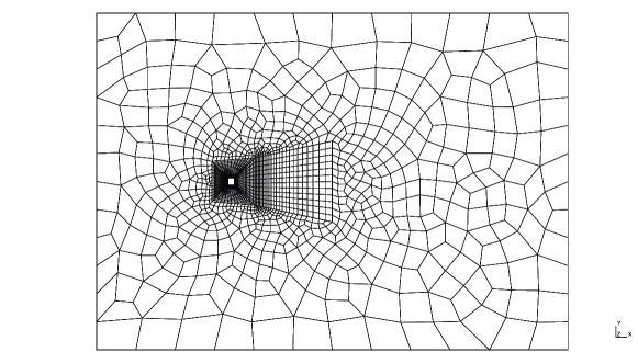
Figure 2: Example of structured/unstructured grids used for the flow past a 3D square cylinder at $Re_{\infty}=2\times 10^{2}$ and $M_{\infty}=0.1$.

We highlight a few observations. First, in all cases an increase in theoretical order of accuracy results in a error reduction on all grids. Secondly, although the convergence rates in model problems are shown on much finer meshes, the computed order of accuracy is very close to the formal value between the medium and fine grids, even for these more realistic meshes.

	$p=1$	rate	$p=2$	rate	$p=3$	rate	$p=4$	rate
Grid 1	4.73e-2	-	2.15e-2	-	9.61e-3	-	4.54e-3	-
Grid 2	1.47e-2	1.69	2.88e-3	2.90	5.83e-4	4.04	1.39e-4	5.02
Grid 3	3.55e-3	2.04	3.66e-4	2.98	3.40e-5	4.10	4.52e-6	4.94

Table 1: $L^{\infty}$ error norm of the velocity component $u_{1}$ at the wall and convergence rates; $t=1$; 3D unsteady laminar flow past a square cylinder at $Re_{\infty}=2\times 10^{2}$ and $M_{\infty}=0.1$.

	$p=1$	rate	$p=2$	rate	$p=3$	rate	$p=4$	rate
Grid 1	7.20e-2	-	2.71e-2	-	1.43e-2	-	5.14e-3	-
Grid 2	1.79e-2	2.01	3.34e-3	3.02	1.10e-3	3.70	1.96e-4	4.71
Grid 3	4.65e-3	1.94	4.20e-4	2.99	7.21e-5	3.93	6.48e-6	4.92

Table 2: $L^{\infty}$ error norm of the velocity component $u_{2}$ at the wall and convergence rates; $t=1$; 3D unsteady laminar flow past a square cylinder at $Re_{\infty}=2\times 10^{2}$ and $M_{\infty}=0.1$.

	$p=1$	rate	$p=2$	rate	$p=3$	rate	$p=4$	rate
Grid 1	2.75e-4	-	1.34e-4	-	1.01e-4	-	8.62e-5	-
Grid 2	5.98e-5	2.20	1.71e-5	2.97	7.92e-6	3.67	3.14e-6	4.78
Grid 3	1.38e-5	2.12	2.03e-6	3.04	5.30e-7	3.90	8.70e-8	5.17

Table 3: $L^{\infty}$ error norm of the velocity component $u_{3}$ at the wall and convergence rates; $t=1$; 3D unsteady laminar flow past a square cylinder at $Re_{\infty}=2\times 10^{2}$ and $M_{\infty}=0.1$.

6.2.2 Vortex shedding

In this section we investigate the vortex shedding and the time variation of the lift and drag coefficients. We compare our results against the data reported by Sohankar et al. [51]. We compute the following quantities: The Strouhal number, $f\,d/|\vec{u}_{\infty}|$, where $f$ is the frequency of the vortex shedding; the time-averaged drag coefficient, $c_{D}$, and the spanwise-averaged root-mean-square (RMS) of the lift coefficient, $c_{L}^{RMS}$. We use the same grids presented in the previous section, and different orders of the polynomial ($p=1,2,3,4$). The results are illustrated in Tables 4, 5, and 6. From these tables, it can be seen that in all cases the accuracy of the results improve by increasing the order of accuracy of the scheme. We also note that, on Grid 3, which is very coarse compared to the typical grids used with second-order FV and FD schemes, fourth- ($p=3$) and fifth-order ($p=4$) accurate entropy stable schemes perform very well. In fact, the aerodynamic coefficients computed with these two discretizations are in very good agreement with the results reported in literature [51].

Solution	$St$	$\langle c_{D}\rangle$	$c_{L}^{RMS}$
SSDC $p=1$	0.098	1.01	0.02
SSDC $p=2$	0.109	1.08	0.06
SSDC $p=3$	0.142	1.19	0.11
SSDC $p=4$	0.151	1.28	0.15
Sohankar et al. [51]	0.160	1.41	0.22

Table 4: Strouhal number, mean drag coefficient, and spanwise-averaged RMS of the lift coefficient for the 3D unsteady laminar flow past a square cylinder at $Re_{\infty}=2\times 10^{2}$ and $M_{\infty}=0.1$; Grid 1.

Solution	$St$	$\langle c_{D}\rangle$	$c_{L}^{RMS}$
SSDC $p=1$	0.128	1.16	0.07
SSDC $p=2$	0.139	1.28	0.13
SSDC $p=3$	0.153	1.36	0.20
SSDC $p=4$	0.159	1.40	0.23
Sohankar et al. [51]	0.160	1.41	0.22

Table 5: Strouhal number, mean drag coefficient, and spanwise-averaged RMS of the lift coefficient for the 3D unsteady laminar flow past a square cylinder at $Re_{\infty}=2\times 10^{2}$ and $M_{\infty}=0.1$; Grid 2.

Solution	$St$	$\langle c_{D}\rangle$	$c_{L}^{RMS}$
SSDC $p=1$	0.134	1.29	0.12
SSDC $p=2$	0.154	1.37	0.19
SSDC $p=3$	0.159	1.40	0.22
SSDC $p=4$	0.159	1.42	0.23
Sohankar et al. [51]	0.160	1.41	0.22

Table 6: Strouhal number, mean drag coefficient, and spanwise-averaged RMS of the lift coefficient for the 3D unsteady laminar flow past a square cylinder at $Re_{\infty}=2\times 10^{2}$ and $M_{\infty}=0.1$; Grid 3.

6.3 Heat entropy flow

In this section we perform a convergence study of the thermal condition to verify that the heat entropy flow at the wall converges to the prescribed value. At $t=100$, we compute the maximum norm $L^{\infty}$ of the error of the quantity $\left[\widetilde{\Theta}_{x_{1}}(5)T_{(\cdot)}\right]$ (see expression (58)) for all the solution points that lie on the solid wall. The entropy flow $g(t)$ is set to $\mathtt{g}(t)=const=0.02$. The results are illustrated in Table 7.

	$p=1$	rate	$p=2$	rate	$p=3$	rate	$p=4$	rate
Grid 1	6.17e-2	-	3.68e-2	-	9.16e-3	-	7.23e-3	-
Grid 2	3.35e-2	0.88	9.95e-3	1.89	1.32e-3	2.79	5.83e-4	3.63
Grid 3	1.63e-2	1.03	2.23e-3	2.16	1.68e-4	2.97	2.59e-5	4.22

Table 7: $L^{\infty}$ error norm of the heat entropy flow at the wall and convergence rates; $\mathtt{g}(t)=const.=0.02$ (see (58)); $t=100$; 3D unsteady laminar flow past a square cylinder at $Re_{\infty}=2\times 10^{2}$ and $M_{\infty}=0.1$.

As for the convergence study on the no-slip boundary conditions, it can be seen that in all cases the accuracy of the results improve by increasing the order of accuracy of the scheme. On this set of grids, the convergence rate of the error associated to the heat entropy flow is $p$.

6.4 Computation of a square cylinder in supersonic freestream

The development of a high-order accurate entropy stable discretization aims to provide the next generation of robust high fidelity numerical solvers for complex fluid flow simulations, for which standard suboptimal algorithms suffer greatly or fail completely. By computing the flow past a 3D square cylinder at $Re_{\infty}=10^{4}$ and $M_{\infty}=1.5$, we provide numerical evidence of such robustness for the complete entropy stable high order spatial discretization. This supersonic flow is characterized by a very large range of length scales, strong shocks and expansion regions that interact with each other, leading to complex flow patterns. During the past three decades, this fluid flow problem has been thoroughly investigated by several researchers for aerodynamic applications (see, for instance, [52, 53, 54]).

The domain of interest spans one square cylinder edge in the $x_{3}$ direction, and at the two planes perpendicular to this coordinate direction, periodic boundary conditions are used. The flow is computed using an unstructured grids with $43,936$ hexahedrons. A fourth-order accurate ($p=3$) entropy stable discretization without absolutely any stabilization technique is used. The body surface is considered adiabatic. The solution is initialized using a uniform flow at $M_{\infty}=1.5$ with zero angle of attack.

At the beginning of the simulation a strong shock is formed in front of the bluff body. Subsequently, the discontinuity moves upstream until it reaches a “stationary” position that is about $2.15$ square cylinder edges far from the frontal surface of the body. During this phase, additional weaker shocks, which originate from the four sharp corners of the body, interact with the subsonic regions formed near the walls. This complicated flow pattern, yields the formation of shock-lets in the wake of the square cylinder. Figure 3 shows a portion of the “high order grid” close to the body and its near-wake region, and the Mach number and density contours at $t=1.5$. It can be seen that relatively small oscillations are generated in front of the shock. This numerical feature is absolutely natural and expected because the solution has been computed with a fourth-order accurate scheme without artificial dissipation or filtering technique. Nevertheless, the simulation remains stable at all time, and the oscillations are always confined in small regions close to the discontinuities.

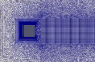
((a)) High order grid in the near-body and near-wake regions.

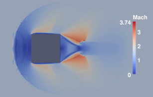
((b)) Mach number; $\Delta M=0.0146$.

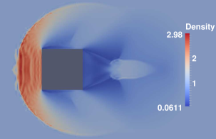
((c)) Density; $\Delta\rho=0.0114$.

Figure 3: Unsteady flow past a 3D square cylinder at $Re_{\infty}=10^{4}$ and $M_{\infty}=1.5$; fourth-order ($p=3$) accurate entropy stable spatial discretization without stabilization technique; $t=1.5$.

In Figures 4 a global view of the “high order grid”, the Mach number, density, temperature and entropy contours at $t=100$ are shown. At $t=100$, the shock has already reached a stationary position, and the flow past the square cylinder is completely unsteady, characterized by subsonic and supersonic regions. The formation of shock-lets in the near wake region are clearly visible.

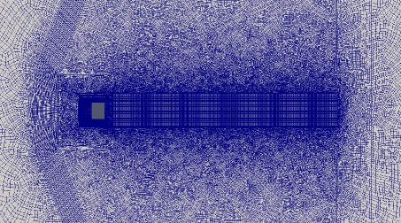
((a)) High order grid.

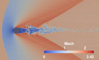
((b)) Mach number; $\Delta M=0.0095$.

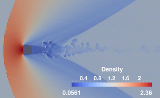
((c)) Density; $\Delta\rho=0.0090$.

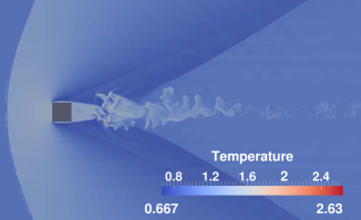
((d)) Temperature; $\Delta T=0.0077$.

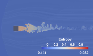
((e)) Entropy; $\Delta s=0.0044$.

Figure 4: Unsteady flow past a 3D square cylinder at $Re_{\infty}=10^{4}$ and $M_{\infty}=1.5$; fourth-order ($p=3$) accurate entropy stable spatial discretization without stabilization technique; $t=100$.

7 Conclusions

Herein, we have shown that no-slip boundary conditions together with a boundary condition on the heat entropy flow, $\left(1/T\,\partial T/\partial n\right)_{wall}$, imply stability for the continuous compressible Navier–Stokes equations. The boundary condition on the heat entropy flow is in complete agreement with the thermodynamic (entropy) analysis of a generic system. An entropy stable numerical procedure is presented for weakly enforcing these solid wall boundary conditions via a penalty approach. The resulting semi-discrete operator mimics exactly the behavior at the continuous level. The proposed non-linear boundary treatment provides a mechanism for ensuring the non-linear stability in the $L^{2}$ norm of the continuous and semi-discretized compressible Navier–Stokes equations. Although discontinuous spectral collocation operators are used in this work, the new boundary conditions are compatible with any diagonal norm summation-by-parts spatial operator, including finite element, finite volume, finite difference, discontinuous Galerkin, and flux reconstruction schemes.

Numerical computations around a three-dimensional square cylinder in the subsonic regime are performed to highlight the accuracy and robustness of the proposed numerical procedure. Measurement of forces on the cylinder showed very good agreement with the results available from the literature. Furthermore, we have shown that the no-slip conditions approach zero to design-order (i.e., the convergence rate is $p+1$), and the heat entropy flow converges to the prescribed boundary value at a rate of $p$.

The robustness of the complete semi-discrete operator (i.e., the entropy stable interior operator coupled with the new boundary treatment) has been demonstrated for the supersonic flow past a three-dimensional square cylinder at $Re_{\infty}=10^{4}$ and $M_{\infty}=1.5$. This test has been successfully computed with a fourth-order accurate method without the need to introduce artificial dissipation, limiting techniques or filtering, for stabilizing the computations, a feat unattainable with several alternative approaches just based on linear analysis.

This work clearly indicates that, although incremental improvements to existing algorithms will continue to improve overall capabilities, the development of novel robust numerical techniques such as entropy preserving or entropy stable schemes and their extension to complex multi-scale and multi-physics problems offers the possibility of radical advances in computational fluid dynamics and computational aerodynamics in terms of robustness, fidelity and efficiency.

Appendix A Coefficient matrices of the viscous flux

The viscous coefficient matrices $c_{ij}^{\prime}$ used to define the viscous fluxes in Cartesian coordinates in (7) are defined as

$$c_{11}^{\prime}=\begin{pmatrix}0&0&0&0&0\\ 0&\frac{4}{3}\mu&0&0&0\\ 0&0&\mu&0&0\\ 0&0&0&\mu&0\\ 0&\frac{4}{3}\mu u_{1}&\mu u_{2}&\mu u_{3}&\kappa\end{pmatrix},\quad c_{12}^{\prime}=\begin{pmatrix}0&0&0&0&0\\ 0&0&-\frac{2}{3}\mu&0&0\\ 0&\mu&0&0&0\\ 0&0&0&0&0\\ 0&\mu u_{2}&-\frac{2}{3}\mu u_{1}&0&0\end{pmatrix},$$

$$c_{13}^{\prime}=\begin{pmatrix}0&0&0&0&0\\ 0&0&0&-\frac{2}{3}\mu&0\\ 0&0&0&0&0\\ 0&\mu&0&0&0\\ 0&\mu u_{3}&0&-\frac{2}{3}\mu u_{1}&0\end{pmatrix},\quad c_{21}^{\prime}=\begin{pmatrix}0&0&0&0&0\\ 0&0&\mu&0&0\\ 0&-\frac{2}{3}\mu&0&0&0\\ 0&0&0&0&0\\ 0&-\frac{2}{3}\mu u_{2}&\mu u_{1}&0&0\end{pmatrix},$$

$$c_{22}^{\prime}=\begin{pmatrix}0&0&0&0&0\\ 0&\mu&0&0&0\\ 0&0&\frac{4}{3}\mu&0&0\\ 0&0&0&\mu&0\\ 0&\mu u_{1}&\frac{4}{3}\mu u_{2}&\mu u_{3}&\kappa\end{pmatrix},\quad c_{23}^{\prime}=\begin{pmatrix}0&0&0&0&0\\ 0&0&0&0&0\\ 0&0&0&-\frac{2}{3}\mu&0\\ 0&0&\mu&0&0\\ 0&0&\mu u_{3}&-\frac{2}{3}\mu u_{2}&0\end{pmatrix},$$

$$c_{31}^{\prime}=\begin{pmatrix}0&0&0&0&0\\ 0&0&0&\mu&0\\ 0&0&0&0&0\\ 0&-\frac{2}{3}\mu&0&0&0\\ 0&-\frac{2}{3}\mu u_{3}&0&\mu u_{1}&0\end{pmatrix},\quad c_{32}^{\prime}=\begin{pmatrix}0&0&0&0&0\\ 0&0&0&0&0\\ 0&0&0&\mu&0\\ 0&0&-\frac{2}{3}\mu&0&0\\ 0&0&-\frac{2}{3}\mu u_{3}&\mu u_{2}&0\end{pmatrix},$$

$$c_{33}^{\prime}=\begin{pmatrix}0&0&0&0&0\\ 0&\mu&0&0&0\\ 0&0&\mu&0&0\\ 0&0&0&\frac{4}{3}\mu&0\\ 0&\mu u_{1}&\mu u_{2}&\frac{4}{3}\mu u_{3}&\kappa\end{pmatrix}.$$

The symmetrized coefficient matrices used in (13) to define the viscous fluxes as a function of the gradient of the entropy variables are found using

$$\widehat{c}_{ij}=c_{ij}\frac{\partial q}{\partial w}=c_{ij}^{\prime}\frac{\partial v}{\partial w}.$$

Therefore, they take the following form:

$$\widehat{c}_{11}=\begin{pmatrix}0&0&0&0&0\\ 0&\frac{4}{3}T\mu&0&0&\frac{4}{3}T\mu u_{1}\\ 0&0&T\mu&0&T\mu u_{2}\\ 0&0&0&T\mu&T\mu u_{3}\\ 0&\frac{4}{3}T\mu u_{1}&T\mu u_{2}&T\mu u_{3}&T^{2}\kappa+\frac{1}{3}T\left(4\mu u_{1}^{2}+3\mu u_{2}^{2}+3\mu u_{3}^{2}\right)\end{pmatrix},$$

$$\widehat{c}_{22}=\begin{pmatrix}0&0&0&0&0\\ 0&T\mu&0&0&T\mu u_{1}\\ 0&0&\frac{4}{3}T\mu&0&\frac{4}{3}T\mu u_{2}\\ 0&0&0&T\mu&T\mu u_{3}\\ 0&T\mu u_{1}&\frac{4}{3}T\mu u_{2}&T\mu u_{3}&T^{2}\kappa+\frac{1}{3}T\left(3\mu u_{1}^{2}+4\mu u_{2}^{2}+3\mu u_{3}^{2}\right)\end{pmatrix},$$

$$\widehat{c}_{33}=\begin{pmatrix}0&0&0&0&0\\ 0&T\mu&0&0&T\mu u_{1}\\ 0&0&T\mu&0&T\mu u_{2}\\ 0&0&0&\frac{4}{3}T\mu&\frac{4}{3}T\mu u_{3}\\ 0&T\mu u_{1}&T\mu u_{2}&\frac{4}{3}T\mu u_{3}&T^{2}\kappa+\frac{1}{3}T\left(3\mu u_{1}^{2}+3\mu u_{2}^{2}+4\mu u_{3}^{2}\right)\end{pmatrix},$$

$$\widehat{c}_{12}=\begin{pmatrix}0&0&0&0&0\\ 0&0&-\frac{2}{3}T\mu&0&-\frac{2}{3}T\mu u_{2}\\ 0&T\mu&0&0&T\mu u_{1}\\ 0&0&0&0&0\\ 0&T\mu u_{2}&-\frac{2}{3}T\mu u_{1}&0&\frac{1}{3}T\mu u_{1}u_{2}\end{pmatrix},\quad\widehat{c}_{13}=\begin{pmatrix}0&0&0&0&0\\ 0&0&0&-\frac{2}{3}T\mu&-\frac{2}{3}T\mu u_{3}\\ 0&0&0&0&0\\ 0&T\mu&0&0&T\mu u_{1}\\ 0&T\mu u_{3}&0&-\frac{2}{3}T\mu u_{1}&\frac{1}{3}T\mu u_{1}u_{3}\end{pmatrix},$$

$$\widehat{c}_{23}=\begin{pmatrix}0&0&0&0&0\\ 0&0&0&0&0\\ 0&0&0&-\frac{2}{3}T\mu&-\frac{2}{3}T\mu u_{3}\\ 0&0&T\mu&0&T\mu u_{2}\\ 0&0&T\mu u_{3}&-\frac{2}{3}T\mu u_{2}&\frac{1}{3}T\mu u_{2}u_{3}\end{pmatrix},$$

where

$$\widehat{c}_{21}=\widehat{c}_{12}^{\top},\quad\widehat{c}_{31}=\widehat{c}_{13}^{\top},\quad\widehat{c}_{32}=\widehat{c}_{23}^{\top}.$$

Appendix B Counter example of non-linear wall boundary conditions

Carrying out the entropy stability analysis by using expression (69), it can be shown that the inviscid penalty in (69) is entropy conservative (see the proof of Theorem 5.1). Therefore, the remaining relation to analyze is

$$\frac{d}{dt}\left\|{S}\right\|^{2}_{\boldsymbol{\mathcal{P}}}\>+\>\mathbf{w}^{\top}\mathcal{P}_{x_{2}x_{3}}\,\mathcal{G}_{(1)}\mathbf{\overline{f}}_{1}^{(V)}+\mathbf{DT}\leq +\mathbf{w}^{\top}\mathcal{P}_{x_{2}x_{3}}\,\mathcal{G}_{(1)}[L]\left(\mathbf{w}-\mathbf{g}^{(NS)}\right).$$ (71)

To obtain a quadratic form in boundary terms we need to borrow from $\mathbf{DT}$:

$$\mathbf{DT} =\sum_{i=1}^{3}\sum_{j=1}^{3}\left(\mathcal{D}_{x_{i}}\mathbf{w}\right)^{\top}\boldsymbol{\mathcal{P}}[\widehat{c}_{ij}]\left(\mathcal{D}_{x_{j}}\mathbf{w}\right)$$ (72)

$$=\begin{pmatrix}\mathcal{D}_{x_{1}}\,\mathbf{w}\\ \mathcal{D}_{x_{2}}\,\mathbf{w}\\ \mathcal{D}_{x_{3}}\,\mathbf{w}\end{pmatrix}^{\top}\begin{pmatrix}\boldsymbol{\mathcal{P}}[\widehat{c}_{11}]&\boldsymbol{\mathcal{P}}[\widehat{c}_{12}]&\boldsymbol{\mathcal{P}}[\widehat{c}_{13}]\\ \boldsymbol{\mathcal{P}}[\widehat{c}_{21}]&\boldsymbol{\mathcal{P}}[\widehat{c}_{22}]&\boldsymbol{\mathcal{P}}[\widehat{c}_{23}]\\ \boldsymbol{\mathcal{P}}[\widehat{c}_{31}]&\boldsymbol{\mathcal{P}}[\widehat{c}_{32}]&\boldsymbol{\mathcal{P}}[\widehat{c}_{33}]\\ \end{pmatrix}\begin{pmatrix}\mathcal{D}_{x_{1}}\,\mathbf{w}\\ \mathcal{D}_{x_{2}}\,\mathbf{w}\\ \mathcal{D}_{x_{3}}\,\mathbf{w}\end{pmatrix}$$

$$=\begin{pmatrix}\mathcal{D}_{x_{1}}\,\mathbf{w}\\ \mathcal{D}_{x_{2}}\,\mathbf{w}\\ \mathcal{D}_{x_{3}}\,\mathbf{w}\end{pmatrix}^{\top}\left(\mathcal{P}_{x_{1}}\right)_{(1)(1)}\begin{pmatrix}\mathcal{P}_{x_{2}x_{3}}[\widehat{c}_{11}]&\mathcal{P}_{x_{2}x_{3}}[\widehat{c}_{12}]&\mathcal{P}_{x_{2}x_{3}}[\widehat{c}_{13}]\\ \mathcal{P}_{x_{2}x_{3}}[\widehat{c}_{21}]&\mathcal{P}_{x_{2}x_{3}}[\widehat{c}_{22}]&\mathcal{P}_{x_{2}x_{3}}[\widehat{c}_{23}]\\ \mathcal{P}_{x_{2}x_{3}}[\widehat{c}_{31}]&\mathcal{P}_{x_{2}x_{3}}[\widehat{c}_{32}]&\mathcal{P}_{x_{2}x_{3}}[\widehat{c}_{33}]\\ \end{pmatrix}\begin{pmatrix}\mathcal{D}_{x_{1}}\,\mathbf{w}\\ \mathcal{D}_{x_{2}}\,\mathbf{w}\\ \mathcal{D}_{x_{3}}\,\mathbf{w}\end{pmatrix}+\widetilde{\mathbf{DT}}$$

$$=\begin{pmatrix}\mathcal{D}_{x_{1}}\,\mathbf{w}\\ \mathcal{D}_{x_{2}}\,\mathbf{w}\\ \mathcal{D}_{x_{3}}\,\mathbf{w}\end{pmatrix}^{\top}\left(\mathcal{P}_{x_{1}}\right)_{(1)(1)}\mathcal{P}^{\prime}\begin{pmatrix}[\widehat{c}_{11}]&[\widehat{c}_{12}]&[\widehat{c}_{13}]\\ [\widehat{c}_{21}]&[\widehat{c}_{22}]&[\widehat{c}_{23}]\\ [\widehat{c}_{31}]&[\widehat{c}_{32}]&[\widehat{c}_{33}]\\ \end{pmatrix}\begin{pmatrix}\mathcal{D}_{x_{1}}\,\mathbf{w}\\ \mathcal{D}_{x_{2}}\,\mathbf{w}\\ \mathcal{D}_{x_{3}}\,\mathbf{w}\end{pmatrix}+\widetilde{\mathbf{DT}},$$

where

$$\mathcal{P}^{\prime}=\textrm{diag}\left(\mathcal{P}_{x_{2}x_{3}},\mathcal{P}_{x_{2}x_{3}},\mathcal{P}_{x_{2}x_{3}}\right),$$

and the scalar $\left(\mathcal{P}_{x_{1}}\right)_{(1)(1)}>0$. Therefore, Equation (71) may be written as

$$\frac{d}{dt} \left\|{S}\right\|^{2}_{\boldsymbol{\mathcal{P}}}+\widetilde{\mathbf{DT}}$$ (73)

$$\leq \>+\>\frac{1}{2}\,\widetilde{\mathbf{w}}^{\top}\widetilde{\mathcal{P}}^{\prime}\begin{pmatrix}[L]&-[\widehat{c}_{11}]&-[\widehat{c}_{12}]&-[\widehat{c}_{13}]\\ -[\widehat{c}_{11}]&-2\left(\mathcal{P}_{x_{1}}\right)_{(1)(1)}\,[\widehat{c}_{11}]&-2\left(\mathcal{P}_{x_{1}}\right)_{(1)(1)}[\widehat{c}_{12}]&-2\left(\mathcal{P}_{x_{1}}\right)_{(1)(1)}\,[\widehat{c}_{13}]\\ -[\widehat{c}_{12}]&-2\left(\mathcal{P}_{x_{1}}\right)_{(1)(1)}\,[\widehat{c}_{12}]&-2\left(\mathcal{P}_{x_{1}}\right)_{(1)(1)}[\widehat{c}_{22}]&-2\left(\mathcal{P}_{x_{1}}\right)_{(1)(1)}\,[\widehat{c}_{23}]\\ -[\widehat{c}_{13]}&-2\left(\mathcal{P}_{x_{1}}\right)_{(1)(1)}\,[\widehat{c}_{13}]&-2\left(\mathcal{P}_{x_{1}}\right)_{(1)(1)}[\widehat{c}_{23}]&-2\left(\mathcal{P}_{x_{1}}\right)_{(1)(1)}\,[\widehat{c}_{33}]\end{pmatrix}\widetilde{\mathbf{w}}$$

$$+\frac{1}{2}\mathbf{w}^{\top}\mathcal{P}_{x_{2}x_{3}}\,\mathcal{G}_{(1)}[L]\,\mathbf{w}-\mathbf{w}^{\top}\mathcal{P}_{x_{2}x_{3}}\,\mathcal{G}_{(1)}[L]\,\mathbf{g}^{(NS)},$$

where

$$\widetilde{\mathcal{P}}^{\prime}=\textrm{diag}\left(\mathcal{P}_{x_{2}x_{3}},\mathcal{P}_{x_{2}x_{3}},\mathcal{P}_{x_{2}x_{3}},\mathcal{P}_{x_{2}x_{3}}\right),$$

and

$$\widetilde{\mathbf{w}}^{\top}=\left((\mathbf{w}_{(0,x_{2},x_{3})}^{\top},\mathbf{0},\left(\mathcal{D}_{x_{1}}\,\mathbf{w}\right)_{(0,x_{2},x_{3})}^{\top},\left(\mathcal{D}_{x_{2}}\,\mathbf{w}\right)_{(0,x_{2},x_{3})}^{\top},\left(\mathcal{D}_{x_{3}}\,\mathbf{w}\right)_{(0,x_{2},x_{3})}^{\top},\mathbf{0}\right).$$ (74)

The bold zeros in (74) indicates that all the numerical states (entropy variables and gradients of the entropy variables) of the nodes which do not lie on the plane $(0,x_{2},x_{3})$ are set to zero.

To bound the time derivative of the entropy we must ensure that each term in (73) is bounded. The first contribution on the RHS is a quadratic term in $\widetilde{\mathbf{w}}$ and dissipative if the large matrix

$$\frac{1}{2}\begin{pmatrix}[L]&-[\widehat{c}_{11}]&-[\widehat{c}_{12}]&-[\widehat{c}_{13}]\\ -[\widehat{c}_{11}]&-2\left(\mathcal{P}_{x_{1}}\right)_{(1)(1)}\,[\widehat{c}_{11}]&-2\left(\mathcal{P}_{x_{1}}\right)_{(1)(1)}[\widehat{c}_{12}]&-2\left(\mathcal{P}_{x_{1}}\right)_{(1)(1)}\,[\widehat{c}_{13}]\\ -[\widehat{c}_{12}]&-2\left(\mathcal{P}_{x_{1}}\right)_{(1)(1)}\,[\widehat{c}_{12}]&-2\left(\mathcal{P}_{x_{1}}\right)_{(1)(1)}[\widehat{c}_{22}]&-2\left(\mathcal{P}_{x_{1}}\right)_{(1)(1)}\,[\widehat{c}_{23}]\\ -[\widehat{c}_{13]}&-2\left(\mathcal{P}_{x_{1}}\right)_{(1)(1)}\,[\widehat{c}_{13}]&-2\left(\mathcal{P}_{x_{1}}\right)_{(1)(1)}[\widehat{c}_{23}]&-2\left(\mathcal{P}_{x_{1}}\right)_{(1)(1)}\,[\widehat{c}_{33}]\end{pmatrix}$$ (75)

is symmetric negative semi-definite. However, to ensure that we only need to construct the following $20\times 20$ matrix,

$$\Gamma=\frac{1}{2}\begin{pmatrix}L&-\widehat{c}_{11}&-\widehat{c}_{12}&-\widehat{c}_{13}\\ -\widehat{c}_{11}&-2\left(\mathcal{P}_{x_{1}}\right)_{(1)(1)}\,\widehat{c}_{11}&-2\left(\mathcal{P}_{x_{1}}\right)_{(1)(1)}\widehat{c}_{12}&-2\left(\mathcal{P}_{x_{1}}\right)_{(1)(1)}\,\widehat{c}_{13}\\ -\widehat{c}_{12}&-2\left(\mathcal{P}_{x_{1}}\right)_{(1)(1)}\,\widehat{c}_{12}&-2\left(\mathcal{P}_{x_{1}}\right)_{(1)(1)}\widehat{c}_{22}&-2\left(\mathcal{P}_{x_{1}}\right)_{(1)(1)}\,\widehat{c}_{23}\\ -\widehat{c}_{13}&-2\left(\mathcal{P}_{x_{1}}\right)_{(1)(1)}\,\widehat{c}_{13}&-2\left(\mathcal{P}_{x_{1}}\right)_{(1)(1)}\widehat{c}_{23}&-2\left(\mathcal{P}_{x_{1}}\right)_{(1)(1)}\,\widehat{c}_{33}\end{pmatrix},$$ (76)

so that it is symmetric negative semi-definite. The matrices $\widehat{c}_{ij},i,j=1,2,3$, in (76) are constructed using the primitive variable at the usual boundary node. The rows and columns of the matrix $\Gamma$ corresponding to the density components are all zero because the first component of the viscous fluxes is zero. Therefore, such rows and columns do not affect the negativity of (76). The matrix $\Gamma$ can be expressed in block form as

$$\Gamma=\begin{pmatrix}A&B\\ B^{\top}&D\end{pmatrix}.$$ (77)

The condition on the five-by-five matrix $L$ that ensures the negative-definiteness of (77) can obtained by requiring that the Schur complement of $\Gamma$ is negative,

$$Schur=A-B\,D^{-1}\,B^{\top}=-\frac{\widehat{c}_{11}+2\,L\,\left(\mathcal{P}_{x_{1}}\right)_{(1)(1)}}{4\left(\mathcal{P}_{x_{1}}\right)_{(1)(1)}}<0.$$ (78)

The inequality in (78) is a sufficient condition because the block matrix $D$ is already well behaved (i.e., it is already symmetric and positive semi-definite). Thus, the Schur complement (78) is smaller than or equal to zero if

$$L\leq-\frac{\widehat{c}_{11}}{2\,\left(\mathcal{P}_{x_{1}}\right)_{(1)(1)}}.$$ (79)

The last two terms on the RHS of expression (73) are the remaining contributions to bound. Such terms can be re-written in a quadratic form as

$$\frac{1}{2}\mathbf{w}^{\top}\mathcal{P}_{x_{2}x_{3}}\,\mathcal{G}_{(1)}[L]\,\mathbf{w}-\mathbf{w}^{\top}\mathcal{P}_{x_{2}x_{3}}\,\mathcal{G}_{(1)}[L]\,\mathbf{g}^{(NS)}= +\frac{1}{2}\left(\mathbf{w}-\mathbf{g}^{(NS)}\right)^{\top}\mathcal{P}_{x_{2}x_{3}}\,\mathcal{G}_{(1)}\,[L]\left(\mathbf{w}-\mathbf{g}^{(NS)}\right)$$ (80)

$$-\frac{1}{2}\left(\mathbf{g}^{(NS)}\right)^{\top}\mathcal{P}_{x_{2}x_{3}}\,\mathcal{G}_{(1)}\,[L]\,\mathbf{g}^{(NS)}.$$

From inequality (79), we know that the matrix $[L]$ is negative definite or negative semi-definite. Therefore, the first term, which is quadratic in $\left(\mathbf{w}-\mathbf{g}^{(NS)}\right)$, is dissipative. However, the second contribution is a positive term and cannot be bounded because it is not only a function of the imposed boundary data $\mathbf{g}^{(NS)}$. In fact, the element in the fifth row and fifth column of the matrix $L$ is non-zero and it is a function of the numerical solution through relation (79) (i.e., through the matrix $\widehat{c}_{11}$ which is built from the numerical state at the boundary node).

References

- [1] J. Dongarra, J. Hittinger, J. Bell, L. Chacón, R. Falgout, M. Heroux, P. Hovland, E. Ng, C. Webster, S. Wild, Applied mathematics research for exascale computing, Tech. Rep. U.S. Department of Energy (2014).
- [2] Z. Wang, K. Fidkowski, R. Abgrall, F. Bassi, D. Caraeni, A. Cary, H. Deconinck, R. Hartmann, K. Hillewaert, H. Huynh, N. Kroll, G. May, P.-O. Persson, B. van Leer, M. Visbal, High-order CFD methods: Current status and perspective, International Journal for Numerical Methods in Fluids 72 (8) (2013) 811–845.
- [3] P.-O. Persson, High-order LES simulations using implicit-explicit Runge–Kutta schemes, in: 49th AIAA Aerospace Sciences Meeting including the New Horizons Forum and Aerospace Exposition, AIAA 2011-684, 2011.
- [4] M. Parsani, G. Ghorbaniasl, C. Lacor, E. Turkel, An implicit high-order spectral difference approach for large eddy simulation, Journal of Computational Physics 229 (14) (2010) 5373–5393.
- [5] R. Hartmann, J. Held, T. Leicht, Adjoint-based error estimation and adaptive mesh refinement for the RANS and turbulence model equations, Journal of Computational Physics 230 (11) (2011) 4268–4284.
- [6] Y. Masayuki, J. M. Modisette, D. L. Darmofal, The importance of mesh adaptation for higher-order discretizations of aerodynamic flows, in: 20th AIAA Computational Fluid Dynamics Conference, AIAA 2011-3852, 2011.
- [7] N. K. Burgess, D. J. Mavriplis, High-order discontinuous Galerkin methods for turbulent high-lift flows, in: Seventh International Conference on Computational Fluid Dynamics (ICCFD7), ICCFD7-4202, 2012.
- [8] G. Lodato, P. Castonguay, A. Jameson, Discrete filter operators for large-eddy simulation using high-order spectral difference methods, International Journal for Numerical Methods in Fluids 72 (2) (2013) 231–258.
- [9] S. Blaise, A. St-Cyr, D. Mavriplis, B. Lockwood, Discontinuous Galerkin unsteady discrete adjoint method for real-time efficient tsunami simulations, Journal of Computational Physics 232 (1) (2013) 416 – 430.
- [10] M. Parsani, M. Bilka, C. Lacor, Large eddy simulation of a muffler with the high-order spectral difference method, in: M. Azaïez, H. El Fekih, J. S. Hesthaven (Eds.), Spectral and high order methods for partial differential equations - ICOSAHOM 2012, Vol. 95 of Lecture Notes in Computational Science and Engineering, Springer International Publishing, 2014, pp. 337–347.
- [11] F. Bassi, L. Botti, A. Colombo, A. Ghidoni, S. Rebay, Implementation of an explicit algebraic Reynolds stress model in an implicit very high-order discontinuous Galerkin solver, in: M. Azaïez, H. El Fekih, J. S. Hesthaven (Eds.), Spectral and high order methods for partial differential equations - ICOSAHOM 2012, Vol. 95 of Lecture Notes in Computational Science and Engineering, Springer International Publishing, 2014, pp. 111–123.
- [12] S. Schoenawa, R. Hartmann, Discontinuous Galerkin discretization of the Reynolds-averaged Navier–Stokes equations with the shear-stress transport model, Journal of Computational Physics 262 (2014) 194–216.
- [13] L. Wang, W. K. Anderson, J. E. Taylor, S. Kapadia, Discontinuous Galerkin and Petrov Galerkin methods for compressible viscous flows, Computers & Fluids 100 (2014) 13–29.
- [14] A. D. Beck, T. Bolemann, D. Flad, H. Frank, G. J. Gassner, F. Hindenlang, C.-D. Munz, High-order discontinuous Galerkin spectral element methods for transitional and turbulent flow simulations, International Journal for Numerical Methods in Fluids 76 (8) (2014) 522–548.
- [15] C. Chen, X. Li, X. Shen, F. Xiao, A high-order conservative collocation scheme and its application to global shallow water equations, Geoscientific Model Development Discussions 7 (4) (2014) 4251–4290.
- [16] J. S. Hesthaven, T. Warburton, Nodal discontinuous Galerkin methods: Algorithms, analysis, and applications, 1st Edition, Springer Publishing Company, Incorporated, 2007.
- [17] J. Zhu, X. Zhong, C.-W. Shu, J. Qiu, Runge–Kutta discontinuous Galerkin method using a new type of WENO limiters on unstructured meshes, Journal of Computational Physics 248 (2013) 200–220.
- [18] T. Hughes, L. Franca, M. Mallet, A new finite element formulation for computational fluid dynamics: Symmetric forms of the compressible Euler and Navier–Stokes equations and the second law of thermodynamics, Computer Methods in Applied Mechanics and Engineering 54 (2) (1986) 223–234.
- [19] E. Tadmor, Entropy stability theory for difference approximations of nonlinear conservation laws and related time-dependent problems, Acta Numerica 12 (2003) 451–512.
- [20] E. Tadmor, The numerical viscosity of entropy stable schemes for systems of conservation laws. I, Mathematics of Computation 49 (179) (1987) 91–103.
- [21] T. C. Fisher, M. H. Carpenter, High-order entropy stable finite difference schemes for nonlinear conservation laws: Finite domains, Tech. Rep. NASA TM 217971 (2013).
- [22] T. C. Fisher, M. H. Carpenter, High-order entropy stable finite difference schemes for nonlinear conservation laws: Finite domains, Journal of Computational Physics 252 (2013) 518–557.
- [23] M. H. Carpenter, T. C. Fisher, High-order entropy stable formulations for computational fluid dynamics, in: 21st AIAA Computational Fluid Dynamics Conference, AIAA 2013-2868, 2013.
- [24] M. Svärd, Third-order accurate entropy-stable schemes for initial-boundary-value conservation laws, Zeitschrift für Angewandte Mathematik und Physik 63 (4) (2012) 599–623.
- [25] M. H. Carpenter, J. Nordström, D. Gottlieb, Revisiting and extending interface penalties for multi-domain summation-by-parts operators, Journal of Scientific Computing 45 (1-3) (2010) 118–150.
- [26] T. C. Fisher, High-order stable multi-domain finite difference method for compressible flows, Ph.D. thesis, Purdue University (2012).
- [27] P. LeFloch, C. Rohde, High-order schemes, entropy inequalities, and nonclassical shocks, SIAM Journal on Numerical Analysis 37 (6) (2000) 2023–2060.
- [28] M. Svärd, H. Özcan, Entropy-stable schemes for the Euler equations with far-field and wall boundary conditions, Journal of Scientific Computing 58 (1) (2014) 61–89.
- [29] B. Gustafsson, H.-O. Kreiss, J. Oliger, Time dependent problems and difference methods, John Wiley & Sons, 1995.
- [30] J. Nordström, M. Svärd, Well-posed boundary conditions for the Navier–Stokes equations, SIAM Journal on Numerical Analysis 43 (3) (2005) 1231–1255.
- [31] M. Svärd, J. Nordström, A stable high-order finite difference scheme for the compressible Navier–Stokes equations: No-slip wall boundary conditions, Journal of Computational Physiscs 227 (10) (2008) 4805–4824.
- [32] J. Berg, J. Nordström, Stable Robin solid wall boundary conditions for the Navier–Stokes equations, Journal of Computational Physics 230 (19) (2011) 7519–7532.
- [33] C.-W. Shu, A brief survey on discontinuous Galerkin methods in computational fluid dynamics, Advances in Mechanics 43 (6) (2013) 541–553.
- [34] P. Vincent, P. Castonguay, A. Jameson, A new class of high-order energy stable flux reconstruction schemes, Journal of Scientific Computing 47 (1) (2011) 50–72.
- [35] R. D. Richtmyer, K. W. Morton, Difference methods for initial-value problems, 2nd Edition, Interscience, 1967.
- [36] H.-O. Kreiss, J. Lorenz, Stability for time-dependent differential equations, Acta Numerica 7 (1998) 203–285.
- [37] P. D. Lax, Hyperbolic systems of conservation laws and the mathematical theory of shock waves, SIAM - Technology & Engineering, 1973.
- [38] J. Smoller, Shock waves and reaction-diffusion equations, 2nd Edition, Springer Science + Business Media New York, 1994.
- [39] A. Harten, On the symmetric form of systems of conservation laws with entropy, Journal of Computational Physiscs 49 (1) (1983) 151–164.
- [40] E. Tadmor, Skew self-adjoint form of systems of conservation laws, Journal of Mathematical Analysis and Applications 103 (2) (1984) 428–442.
- [41] C. M. Dafermos, Hyperbolic conservation laws in continuum physics, Springer-Verlag, Berlin, 2010.
- [42] S. K. Godunov, An interesting class of quasilinear systems, Dokl. Akad. Nauk SSSR 139 (3) (1961) 521–523.
- [43] H.-O. Kreiss, J. Lorenz, Initial boundary value problems and the Navier–Stokes equations, Academic Press, New York, 1989.
- [44] A. Bejan, Entropy generation minimization, 1st Edition, CRC, Boca Raton, New York, 1996.
- [45] M. Parsani, M. H. Carpenter, E. J. Nielsen, Entropy stable wall boundary conditions for the compressible Navier–Stokes equations, Tech. Rep. NASA TM 218282 (2014).
- [46] M. H. Carpenter, T. C. Fisher, E. J. Nielsen, S. H. Frankel, Entropy stable spectral collocation schemes for the Navier–Stokes equations: Discontinuous interfaces, Tech. Rep. NASA TM 218039 (2013).
- [47] F. Ismail, P. L. Roe, Affordable, entropy-consistent Euler flux functions II: Entropy production at shocks, Journal of Computational Physics 228 (15) (2009) 5410–5436.
- [48] M. H. Carpenter, T. C. Fisher, E. J. Nielsen, S. H. Frankel, Entropy stable spectral collocation schemes for the Navier–Stokes equations: Discontinuous interfaces, SIAM Journal on Scientific Computing (2014), In Press.
- [49] M. L. Merriam, An entropy-based approach to nonlinear stability, Tech. Rep. NASA TM 101086 (1989).
- [50] C. Norberg, Flow around rectangular cylinders: Pressure forces and wake frequencies, Journal of Wind Engineering & Industrial Aerodynamics 49 (1-3) (1993) 187–196.
- [51] A. Sohankar, C. Norberg, L. Davison, Numerical simulation of flow past a square cylinder, in: 3rd ASME/JSME Joint Fluids Engineering Conference, FEDSM99-7172, 1999.
- [52] T. Nakagawa, Mach number effects on vortex shedding of a square cylinder and thick symmetrical airfoil arranged in tandems, Proceeding of the Royal Society London A 407 (1833) (1986) 283–297.
- [53] T. Nakagawa, Vortex shedding behind a square cylinder in transonic flows, Journal of Fluid Mechanics 178 (1987) 303–323.
- [54] T. Birch, S. A. Prince, G. M. Simpson, An experimental and computational study of the aerodynamics of a square cross-section body at supersonic speeds, Tech. Rep. RTO-MP-069(I), DERA (2003).