Supplementary Material for “Inference for a two-component mixture of symmetric distributions under log-concavity”

Inference for a two-component mixture of symmetric distributions under log-concavity

Inference for a two-component mixture of symmetric distributions under log-concavity

Abstract

In this article, we revisit the problem of estimating the unknown zero-symmetric distribution in a two-component location mixture model, considered in previous works, now under the assumption that the zero-symmetric distribution has a log-concave density. When consistent estimators for the shift locations and mixing probability are used, we show that the nonparametric log-concave Maximum Likelihood estimator (MLE) of both the mixed density and that of the unknown zero-symmetric component are consistent in the Hellinger distance. In case the estimators for the shift locations and mixing probability are $\sqrt{n}$-consistent, we establish that these MLE’s converge to the truth at the rate $n^{-2/5}$ in the $L_{1}$ distance. To estimate the shift locations and mixing probability, we use the estimators proposed by Hunter et al. (2007). The unknown zero-symmetric density is efficiently computed using the R package logcondens.mode.

Abstract

In this article, we revisit the problem of estimating the unknown zero-symmetric distribution in a two-component location mixture model, considered in previous works, now under the assumption that the zero-symmetric distribution has a log-concave density. When consistent estimators for the shift locations and mixing probability are used, we show that the nonparametric log-concave Maximum Likelihood estimator (MLE) of both the mixed density and that of the unknown zero-symmetric component are consistent in the Hellinger distance. In case the estimators for the shift locations and mixing probability are $\sqrt{n}$-consistent, we establish that these MLE’s converge to the truth at the rate $n^{-2/5}$ in the $L_{1}$ distance. To estimate the shift locations and mixing probability, we use the estimators proposed by Hunter et al. (2007). The unknown zero-symmetric density is efficiently computed using the R package logcondens.mode.

Abstract

This supplement contains proofs and other technical material for “Inference for a mixture of symmetric distributions under log-concavity”. Reference numbers to equations, theorems, or other statements in that document have a unified numbering system with this document. The bibliography is shared and found at the end of the main document.

1 Introduction

Let us assume that $X_{1},\ldots,X_{n}$ are independent and identically distributed (i.i.d.) draws from a mixture distribution, with cumulative distribution function (cdf) $G^{0}$ given by

$$G^{0}(x)=\sum_{i=1}^{k}\pi_{i}^{0}F_{i}^{0}(x),\;\;\;\;x\in\mathbb{R},$$ (1)

for some integer $k\geq 2$, where $F_{i}^{0}$ are cdfs, $\pi_{i}^{0}\geq 0,$ and $\sum_{i=1}^{k}\pi_{i}^{0}=1$. Such mixture distributions are very common in statistical modeling, in part because a variety of data generating frameworks lead to mixture models; for instance, one common approach to clustering problems leads to estimation of a mixture density (Fraley and Raftery, 2002). Another reason for this popularity is that they are very flexible and many distributions can be well approximated by some mixture model (see, e.g., Everitt and Hand (1981), Titterington et al. (1985), or McLachlan and Peel (2000)).

In this paper, we revisit the semi-parametric mixture model already studied by Bordes et al. (2006) and Hunter et al. (2007). In this model, it is assumed that the mixing distributions $F_{i},1\leq i\leq k$ in (1) are such that

$$F_{i}(x)=F^{0}(x-u_{i}^{0})$$

for $u_{i}^{0}\in\mathbb{R}$, $i=1,\ldots,k$, and $F^{0}$ is a distribution function restricted to be symmetric about $0$, i.e.  $F^{0}(-x)=1-F^{0}(x-)$. This model was also studied more recently by Butucea and Vandekerkhove (2014). All of these authors have actually focused on the case $k=2$:

$$G^{0}(x)=\pi^{0}F^{0}(x-u_{1}^{0})+(1-\pi^{0})F^{0}(x-u_{2}^{0}),\;\;\;\;x\in\mathbb{R}.$$ (2)

This is still, in fact, a flexible model which is useful in many scenarios (see our data applications in Section 6). As the main goal is to estimate the mixing parameters and the mixing component $F^{0}$, it is crucial to be assured that there exists a unique solution $(\pi^{0},u^{0}_{1},u^{0}_{2},F^{0})$ for a given $G^{0}$ determined by (2). Bordes et al. (2006) and Hunter et al. (2007) were able to establish that identifiability holds under some suitable conditions on the mixing parameters. Their result states that if $u_{1}^{0}<u_{2}^{0}$ and $\pi^{0}\notin\left\{0,1/2,1\right\}$, then $G^{0}$ given (2) is identifiable for any zero-symmetric distributions $F^{0}$. Furthermore, the condition is necessary and sufficient since any distribution $G^{0}$ that is symmetric about its median clearly cannot be $2$-identifiable; see Theorem 2 of Hunter et al. (2007).

After having shown identifiability, Hunter et al. (2007) put their focus on estimating $(\pi^{0},u_{1}^{0},u_{2}^{0},F^{0})$. They have shown that their estimator of the parametric component $(\pi^{0},u_{1}^{0},u_{2}^{0})$ is consistent and asymptotically normal. However, the obtained estimator of $F^{0}$ is not even guaranteed to have the properties of a genuine cdf (i.e., it is not necessarily nondecreasing). On the other hand, Bordes et al. (2006), Butucea and Vandekerkhove (2014), and Chee and Wang (2013) use a KDE approach to estimation of $F^{0}$. The resulting estimators are proper distribution functions, but the procedures involve a model-selection procedure (cross-validation or Akaike or Bayesian information criterion) to choose the tuning parameter. The estimators of Hunter et al. (2007) and Butucea and Vandekerkhove (2014) for the mixture parameters are shown to converge weakly to a multivariate Gaussian at the parametric rate $n^{-1/2}$ under some regularity conditions on $F^{0}$ which are related to smoothness in the case of Butucea and Vandekerkhove (2014). Bordes et al. (2006) obtain also a convergence rate under smoothness assumptions, but their rate of convergence is much slower (of order $n^{-1/4+\alpha}$, for any $\alpha>0$). Bordes et al. (2006) show that the same rates of convergence are inherited by their kernel estimator of $F^{0}$ in the supremum norm, under the assumption that the location parameters $u^{0}_{1}$ and $u^{0}_{2}$ are unknown. If $F^{0}$ is assumed to admit a density $f^{0}$, then Bordes et al. (2006) provide only almost sure consistency in the supremum norm. For their kernel estimator, Butucea and Vandekerkhove (2014)) obtain, for pointwise convergence, a rate of order $n^{-(2\beta-1)/(4\beta)}$ in the quadratic risk assuming smoothness of level $\beta>1/2$ and assuming that the bandwidth is chosen optimally (the authors suggest using cross validation).

Hence, the proposed estimators of $F^{0}$ in the aforementioned works suffer various practical difficulties, including slow rates of convergence (or as-of-yet unknown rates) for it or its density, the estimator not being a proper cdf, or the need for model-selection procedures to choose a tuning parameter. Our goal in this paper is to circumvent those issues by constructing an estimator of the density $f^{0}$ which

• converges to the truth with a provably good convergence rate,

• can be efficiently computed,

• does not require a tuning parameter, and furthermore,

• is unimodal.

Unimodality is a natural constraint to enforce; when using a mixture model, it is somewhat unnatural to imagine a multimodal mixture component density. However, using unimodality involves some technical difficulties: enforcing unimodality on $f^{0}$ is not directly feasible, because the class of unimodal densities is too large and the MLE of a unimodal density fails to exist even in the simple one-dimensional setting (with no mixing). We propose instead to assume that $f^{0}$ satisfies the shape constraint of log-concavity (i.e., $\log f^{0}$ is concave).

Log-concave functions are always unimodal, and have been used to great success in nonparametric modeling. Unlike the class of unimodal densities, the log-concave class admits an MLE (Walther, 2002). Many papers have studied the log-concave MLE on $\mathbb{R}$ or $\mathbb{R}^{d}$ and much is already known about its large sample properties, both local and global; see e.g. Pal et al. (2007), Dümbgen and Rufibach (2009), Balabdaoui et al. (2009), Cule and Samworth (2010), Cule et al. (2010), Dümbgen et al. (2011), Schuhmacher and Dümbgen (2010), Chen and Samworth (2013), Doss and Wellner (2015), and Kim and Samworth (2014). Balabdaoui et al. (2013) studied asymptotics and confidence intervals of the discrete log-concave MLE of a probability mass function in the well- and misspecified settings. Dümbgen et al. (2010), Rufibach (2007) and Dümbgen and Rufibach (2011) study algorithms for computation of the MLE, allowing unequal weights to be assigned to the observations, an important feature of which we will take advantage.

In the present context, we need to consider the class of zero-symmetric log-concave densities on $\mathbb{R}$, which has not been considered before. To do so, we note that if $f$ is zero-symmetric and log-concave on $\mathbb{R}$, then $f^{+}(t):=2f(t)\mathbb{I}_{t\in[0,\infty)}$ is log-concave with mode at 0. Thus, through a simple transformation of the data, it can be shown that the original estimation problem is equivalent to maximizing the log-likelihood over the class of log-concave densities on $[0,\infty)$ with mode at 0. We can then compute the maximum of the log-likelihood easily by alternating between the EM algorithm (Dempster et al., 1977) and the active set algorithm provided in the R package logcondens.mode which computes the log-concave MLE with a fixed mode. We use the fact that the active set algorithm allows for unequal weights to be assigned to the data points: here, the weights assigned are proportional to the posterior probabilities from the EM algorithm.

We are able to show that the zero-symmetric log-concave MLE converges in probability to the true zero-symmetric log-concave component density in the Hellinger distance and in the supremum norm on sets of continuity of the true density. Furthermore, it can be shown that our estimator converges to the truth at the rate $n^{-2/5}$ in the $L_{1}$-distance. Although the risk measure we use here is different from the one considered by Butucea and Vandekerkhove (2014), it seems that the rate of convergence of our MLE, when the true mixture component is log-concave, is faster than that given in their Theorem 4 for their KDE when the smoothness parameter $\beta$ satisfies $\beta\in(1/2,5/2)$. Note for an estimator $\hat{g}_{n}$ of $g_{0}$ in the direct density estimation problem based on i.i.d. observations from $g_{0}$ (as opposed to the mixture setting) when $g_{0}$ has smoothness $\beta$ the optimal pointwise rate of convergence of $|\hat{g}_{n}(x_{0})-g_{0}(x_{0})|$ at a fixed point $x_{0}$ is $n^{-\beta/(2\beta+1)}$ (Stone, 1980). Note also that Dümbgen and Rufibach (2009) find a rate of convergence of $(\log n)^{\frac{\beta}{2\beta+1}}n^{-\frac{\beta}{2\beta+1}}$ in the uniform norm on compact sets for the log-concave MLE, in the direct density estimation problem, when the true density $g_{0}$ is log-concave and also lies in a Hölder class with smoothness $\beta$, i.e.

$$|g_{0}(x)-g_{0}(y)| \leq L|x-y|,\ \ \textrm{if $\beta=1$}$$

$$|g_{0}^{\prime}(x)-g_{0}^{\prime}(y)| \leq L|x-y|^{\beta-1},\ \ \textrm{if $\beta>1$}$$

for some $L>0$. This rate is optimal for nonparametric estimation with smoothness $\beta$ (the log factor being due to the supremum norm (Khas’minskii, 1978)), and no bandwidth needs to be chosen.

We note that, although we refer to our estimator as the log-concave MLE, we do not use a “pure” maximum likelihood approach since we feed in other estimators of $(\pi^{0},u_{1}^{0},u_{2}^{0})$ to our likelihood, which we maximize to estimate $f^{0}$ and thus $g^{0}$, the density of the mixed distribution $G^{0}$. An alternative approach is to estimate both the parametric and nonparametric components simultaneously by maximum likelihood. However, there are many additional difficulties in that approach, due to the complicated non-concave nature of the log-likelihood function; see Section 2.

We also note that we are not the first to use log-concavity in mixture modeling; Chang and Walther (2007) and Eilers and Borgdorff (2007) consider univariate mixtures of log-concave densities, and Cule et al. (2010) consider multivariate mixtures of log-concave densities. However, in none of those settings was symmetry imposed, perhaps because the authors were not worried about the (often fundamental) question of identifiability. Thus, their work does not directly apply in our setting.

The paper will be structured as follows. In Section 2 we establish existence of the MLE and provide a necessary condition for a candidate to be equal to the estimator. In Section 3, we establish consistency in the Hellinger distance. This implies other forms of consistency by the results of Cule and Samworth (2010). The techniques we used are re-adapted from Pal et al. (2007), Cule and Samworth (2010) and Schuhmacher and Dümbgen (2010) to deal with the additional difficulties of a mixture model. In Section 4, we find that the MLEs of $f^{0}$ and $g^{0}$ converge to the truth at a rate of order $n^{-2/5}$. In Section 5, we develop a likelihood ratio procedure based on our estimator in the problem of testing absence of mixing. We also consider the problem of clustering where we use the estimators of the posterior probabilities obtained via our log-concave MLE. In both problems, we compare our method to alternative or existing approaches. In Section 6, we present two data applications. Section 7 gathers some conclusions. Proofs and technical details can be found in the online supplementary material.

2 The model and estimation via Maximum likelihood

Let $X_{1},\ldots,X_{n}$ to be $n$ independent observations assumed to come from the location mixture with cdf $G^{0}$ which we now assume has a density, given by

$$g^{0}(x)=\pi^{0}f^{0}(x-u^{0}_{1})+(1-\pi^{0})f^{0}(x-u^{0}_{2}),$$ (3)

for some $\pi^{0}\in(0,1)\setminus\{1/2\}$, $u^{0}_{1},u^{0}_{2}\in\mathbb{R}$ such that $u^{0}_{1}\neq u^{0}_{2}$. We assume that $f^{0}$ is a zero-symmetric log-concave density, i.e. $f^{0}\in{\cal SLC}_{1}$ where

$${\cal SLC}_{1}:={\cal SLC}\cap\left\{f:\int_{\mathbb{R}}f(u)du=1\right\},\;\mbox{and}\;{\cal SLC}:=\left\{e^{\psi}:\psi\in{\cal SC}\right\},$$

and ${\cal SC}$ is the class of concave functions on $\mathbb{R}$ that are upper semi-continuous (“closed”) and proper (Rockafellar, 1970), and satisfy $\psi(x)=\psi(-x)$. The upper semi-continuity condition is made only for the purpose of uniqueness. Then

$$L(\pi,u_{1},u_{2},f):=\sum_{j=1}^{n}\log\Big{(}\pi f(X_{j}-u_{1})+(1-\pi)f(X_{j}-u_{2})\Big{)}.$$ (4)

is the log-likelihood in this problem. In the case of estimation of a log-concave density on $\mathbb{R}$, the log-likelihood is a concave function (Pal et al. (2007), Rufibach (2007), Dümbgen and Rufibach (2009)). However, Dümbgen et al. (2010) study a semiparametric model incorporating log-concavity and find a non-concave likelihood; see their Section 3.3 including a plot on page 18. Unfortunately, our objective function $L$ is also far from concave. Consider order statistics $X_{(1)},\ldots,X_{(n)}$, a fixed $\pi\in(0,1)\setminus\{1/2\}$, and (zero-symmetric log-concave) $f$ with support given by $\operatorname{supp}(f)=[-s,s]$ and $\inf_{x\in\operatorname{supp}(f)}f(x)>0$. Assume $u_{1}<u_{2}$ are such that $[u_{1}-s,u_{1}+s]\cup[u_{2}-s,u_{2}+s]\supset[X_{(1)},X_{(n)}]$ so that $L(\pi,u_{1},u_{2},f)>-\infty.$ Let $j:=\min\left\{i:X_{(i)}>u_{2}-s\right\}$ be the index of the smallest order statistic contained in the support of the second component, and let $\tilde{\delta}:=X_{(j)}-(u_{2}-s)$. Then not only does $L(\pi,u_{1},\cdot,f)$ fail to be concave, but it is in fact discontinuous at $u_{2}+\tilde{\delta}$.

We now describe our estimation approach. Let $\widecheck{\pi}_{n},\widecheck{u}_{1,n},\widecheck{u}_{2,n}$ be estimators of $\pi,u_{1},u_{2}$, where we assume $\widecheck{\pi}_{n}\in(0,1)\setminus\left\{1/2\right\}$ and $\widecheck{u}_{1,n}<\widecheck{u}_{2,n}$. We will generally think of these estimators as being $\sqrt{n}$-consistent. We will then consider maximizing the log-likelihood

$$f\mapsto\sum_{j=1}^{n}\log\Big{(}\widecheck{\pi}_{n}f(X_{j}-\widecheck{u}_{1,n})+(1-\widecheck{\pi}_{n})f(X_{j}-\widecheck{u}_{2,n})\Big{)}$$ (5)

over $\mathcal{SLC}_{1}$. Using the Lagrange penalty term introduced by Silverman (1982), this is equivalent to maximizing the criterion $\Phi_{n}$ defined as

$$\Phi_{n}(\psi)=\frac{1}{n}\sum_{j=1}^{n}\log\Big{[}\widecheck{\pi}_{n}e^{\psi(X_{i}-\widecheck{u}_{1,n})}+(1-\widecheck{\pi}_{n})e^{\psi(X_{i}-\widecheck{u}_{2,n})}\Big{]}-\int_{\mathbb{R}}e^{\psi(x)}dx$$

over $\mathcal{SC}$. We will abusively use the term MLE for our estimators of $f^{0}$ and $g^{0}$ despite the fact that the mixing parameters $(\pi,u_{1},u_{2})$ are not a part of the space over which the likelihood is maximized. In the next proposition we establish existence of the MLE, and describe its nature.

Proposition 2.1

The criterion $\Phi_{n}$ admits a maximizer $\widehat{\psi}_{n}$. Furthermore, the following holds true almost surely, letting $\widehat{f}_{n}=e^{\widehat{\psi}_{n}}$.

• $\widehat{f}_{n}$ is in $\mathcal{SLC}_{1}$.

• For $i=1,\ldots,n$, let

  $$Z_{2i-1}=|X_{i}-\widecheck{u}_{1,n}|\mbox{ and }Z_{2i}=|X_{i}-\widecheck{u}_{2,n}|.$$ (6)

  Then, on $[0,\infty)$ the MLE $\widehat{\psi}_{n}$ changes slope only at points belonging to the set

  $$\big{\{}Z_{1},Z_{2},\ldots,Z_{2n-1},Z_{2n}\big{\}}.$$

  Furthermore, $\widehat{\psi}_{n}^{\prime}(0)=0$, and $\widehat{\psi}_{n}(x)=-\infty$ if and only if $x\notin[-Z_{(2n)},Z_{(2n)}]$ where $Z_{(2n)}$ is the largest order statistic of $Z_{1},Z_{2},\ldots,Z_{2n-1},Z_{2n}$.

The MLE of $f$ will be denoted by $\widehat{f}_{n}$ throughout, and that of $g$ by $\widehat{g}_{n}$. In the following, we give a necessary condition for a log-concave function $f=\exp(\psi)$ to be the MLE.

Proposition 2.2 is interesting to compare with the characterization of Dümbgen and Rufibach (2009) for the log-concave MLE. The result is also useful in combination with the EM-algorithm described below as its non-fulfillment indicates that convergence is not yet reached.

Proposition 2.2

Let $\psi$ be a zero-symmetric concave function on $\mathbb{R}$ such that $\psi(x)=-\infty$ if and only if $x\notin[-Z_{(2n)},Z_{(2n)}]$ where $Z_{(2n)}$ is defined in Proposition 2.1, and $\psi^{\prime}(0)=0$. If $\exp(\psi)=\widehat{f}_{n}$ is the MLE, then for any real zero-symmetric function $\Delta$ such that $\psi+\epsilon\Delta\in\mathcal{SC}$ for some $\epsilon>0$ we have that

$$\frac{1}{n}\sum_{i=1}^{n}\Big{\{}\widehat{p}_{n}(X_{i})\Delta(X_{i}-\widecheck{u}_{1,n})+(1-\widehat{p}_{n}(X_{i}))\Delta(X_{i}-\widecheck{u}_{2,n})\Big{\}}\leq\int_{\mathbb{R}}\widehat{f}_{n}(x)\Delta(x)dx$$ (7)

where

$$\widehat{p}_{n}(X_{i})=\frac{\widecheck{\pi}_{n}\widehat{f}_{n}(X_{i}-\widecheck{u}_{1,n})}{\widecheck{\pi}_{n}\widehat{f}_{n}(X_{i}-\widecheck{u}_{1,n})+(1-\widecheck{\pi}_{n})\widehat{f}_{n}(X_{i}-\widecheck{u}_{2,n})}=\frac{\widecheck{\pi}_{n}\widehat{f}_{n}(X_{i}-\widecheck{u}_{1,n})}{\widehat{g}_{n}(X_{i})},$$ (8)

for $i=1,\ldots,n$.

Next, we give the condition in (7) under an alternative form. Dümbgen and Rufibach (2009) shows that the log-concave MLE is uniquely characterized by the fact that the first integral of the cdf of the MLE stays below the first integral of the empirical distribution, while touching it exactly at the points where the logarithm of the MLE changes slope. To derive a related result, let $\widehat{\mathbb{F}}_{n}$ denote the cdf of the discrete distribution putting mass $\widehat{p}_{n}(X_{i})/n$ at $Z_{2i-1}$ and $(1-\widehat{p}_{n}(X_{i}))/n$ at $Z_{2i}$ for $i=1,\ldots,n$, where $\widehat{p}_{n}(X_{i})$ was defined in (8) and $Z_{i}$ was defined in (6). That is,

$$\widehat{\mathbb{F}}_{n}=\frac{1}{n}\sum_{i=1}^{n}\left(\widehat{p}_{n}(X_{i})\delta_{Z_{2i-1}}+(1-\widehat{p}_{n}(X_{i}))\delta_{Z_{2i}}\right)$$

where $\delta_{x}(t)=1_{\{[x,\infty)\}}(t)$. Let $\widehat{f}^{+}_{n}(x)=2\widehat{f}_{n}(x)1_{x\in[0,\infty)}$, $\widehat{\psi}_{n}^{+}=\log(\widehat{f}_{n}^{+})$ and let $\widehat{F}^{+}_{n}$ be the cdf of $\widehat{f}^{+}_{n}$.

Proposition 2.3

If $\widehat{f}_{n}$ is the MLE of the component $f^{0}\in\mathcal{SLC}_{1}$ then

$$\int_{0}^{z}\widehat{F}^{+}_{n}(x)dx\begin{cases}\leq\int_{0}^{z}\widehat{\mathbb{F}}_{n}(x)dx,\ \textrm{for $z\in[0,Z_{(2n)}]$}\\ =\int_{0}^{z}\widehat{\mathbb{F}}_{n}(x)dx,\ \textrm{if $\widehat{\psi}^{+}_{n}(z-)>\widehat{\psi}^{+}_{n}(z+)$}.\end{cases}$$ (9)

3 Consistency

The main result of this section is to establish consistency in the Hellinger distance of the MLEs $\widehat{g}_{n}$ and $\widehat{f}_{n}$ as $n\to\infty$, where the Hellinger distance is defined by

$$H(p,q):=\sqrt{(1/2)\int\left(\sqrt{p(x)}-\sqrt{q(x)}\right)^{2}dx}.$$

We will also find consistency for $\widehat{f}_{n}$ in certain exponentially weighted metrics. Our approach to the problem follows the idea of Pal et al. (2007) and Dümbgen and Rufibach (2009) but will require handling carefully the extra complexity induced by the mixture. As in Pal et al. (2007), Cule and Samworth (2010) and Schuhmacher and Dümbgen (2010), we will first need to show that the MLE of the mixed density and hence the MLE of the log-concave component are bounded. Here, the claimed boundedness will be only in probability, which is weaker than the almost sure boundedness proved in the aforementioned articles. Those articles, however, were able to take advantage of the fact that the level sets of a bounded unimodal function are convex and compact; such a statement does not hold if we consider a mixture of two unimodal functions instead of a single unimodal function, even if the two components are log-concave. So, instead of studying how the empirical distribution behaves over the class of compact intervals, we will instead need to study its behavior over more complicated classes of functions. This is what is done in Propositions B.2 and B.3.

Theorem 3.1

Let $g^{0}$ be as in (3) and $\widehat{g}_{n}$ be the MLE of $g^{0}$. Then we have that

$$H(\widehat{g}_{n},g^{0})=o_{p}(1).$$

Consistency of the log-concave component, $\widehat{f}_{n}$, follows now from Theorem 3.1.

Corollary 3.1

Let $f^{0}$ denote again the true log-concave zero-symmetric density. Then,

$$H(\widehat{f}_{n},f^{0})=o_{p}(1),$$

and for any $a\in(0,a_{0})$ such that $f^{0}(x)\leq\exp(-a_{0}x+b)$ for some $b\in\mathbb{R}$, then

$$\int_{\mathbb{R}}e^{at}|\widehat{f}_{n}(t)-f^{0}(t)|=o_{p}(1),$$

and

$$\sup_{t\in[-A,A]}e^{at}|\widehat{f}_{n}(t)-f^{0}(t)|=o_{p}(1).$$

on any continuity set $[-A,A]$ of $f^{0}$, where $A$ may be $\infty$ if $f^{0}$ is continuous on all of $\mathbb{R}$.

4 Rates of convergence

In this section, we aim at refining the convergence result obtained in the previous section to attain a rate of convergence for both $\widehat{f}_{n}$ and $\widehat{g}_{n}$ in the $L_{1}$ distance. To this goal, we need first to recall some definitions from empirical processes theory. Given a class of functions $\mathcal{F}$, the bracketing number of $\mathcal{F}$ under some distance $\|\cdot\|$ is defined as

$$N_{[\ ]}(\epsilon,\mathcal{F},\|\cdot\|)=\min\Big{\{}k:\exists\ \underline{f}_{1},\bar{f}_{1},\ldots,\underline{f}_{k},\bar{f}_{k}\ \textrm{s.t.}\|\underline{f}_{i}-\bar{f}_{j}\|\leq\epsilon,\mathcal{F}\subset\cup_{i=1}^{k}[\underline{f}_{i},\bar{f}_{i}]\Big{\}}$$

where $[l,u]=\{f:\in\mathcal{F}:l\leq f\leq u\}$. In this section, we refine the consistency result above by deriving the rate of convergence of the MLE’s $\widehat{g}_{n}$ and $\widehat{f}_{n}$ of the mixed density and the zero-symmetric log-concave component respectively.

For fixed $M>0$, $a_{0}<b_{0}$ and $\delta\in\left(0,(b_{0}-a_{0})/2\right)$, consider the class of functions

$$\mathcal{G} = \Bigg{\{}\lambda f(\cdot-a)+(1-\lambda)f(\cdot-b),\ f\in\mathcal{SLC},\ f(0)\in[1/M,M],\lambda\in[0,1],$$

$$\hskip 5.69046pt\ (a,b)\in[a_{0}-\delta,a_{0}+\delta]\times[b_{0}-\delta,b_{0}+\delta]\Bigg{\}}.$$

Here, the parameters $a_{0}$ and $b_{0}$ play the role of the true location shifts $u^{0}_{1}$ and $u^{0}_{2}$. Consistency of the estimates $\widecheck{u}_{1,n}$ and $\widecheck{u}_{2,n}$ ensures that they are stay within distance $2\delta$ from the truth with increasing probability. Also, uniform consistency of the log-concave MLE, $\widehat{f}_{n}$, on continuity sets of $f^{0}$ implies consistency at the point 0 (the common mode of $f^{0}$ and $\widehat{f}_{n}$). Thus, we can find $M>0$ such that $\widehat{f}_{n}(0)\in[1/M,M]$ with increasing probability. The following proposition gives a bound on the bracketing entropy for the class $\mathcal{G}$.

Proposition 4.1

For $\epsilon\in(0,\epsilon_{0}]$, we have that

$$\log N_{[\ ]}(\epsilon,\mathcal{G},H)\lesssim\frac{1}{\sqrt{\epsilon}}$$

where $\epsilon_{0}$ and $\lesssim$ depend only on $a_{0},b_{0},\delta$ and $M$.

Now, we are ready to state our main theorem. We find a rate of convergence of at least $n^{-2/5}$ in the $L_{1}$ norm, both for $\widehat{f}_{n}$ and $\widehat{g}_{n}$. Although we consider $L_{1}$ and Butucea and Vandekerkhove (2014) consider $L_{2}$ distance, the rate of Theorem 4.1 is an improvement over the corresponding $L_{2}$ rate $n^{-(2\beta-1)/(4\beta)}$ of Butucea and Vandekerkhove (2014) whenever $\beta<5/2$. (Note that (log-)concave functions are Lebesgue-almost-everywhere twice differentiable by Alexandrov’s theorem (Niculescu and Persson, 2006), so roughly correspond to $\beta$ being $2$ or larger.)

Theorem 4.1

Let $\widehat{f}_{n}$ and $\widehat{g}_{n}$ be again the MLE’s of the zero-symmetric log-concave component and mixed density respectively. If $\sqrt{n}(\widecheck{u}_{1,n}-u^{0}_{1})=O_{p}(1)$, $\sqrt{n}(\widecheck{u}_{2,n}-u^{0}_{1})=O_{p}(1)$, and $\sqrt{n}(\widecheck{\pi}_{n}-\pi^{0})=O_{p}(1)$, then

$$L_{1}\big{(}\widehat{f}_{n},f^{0}\big{)}=O_{p}\big{(}n^{-2/5}\big{)},\ \textrm{and}\ \ L_{1}\big{(}\widehat{g}_{n},g^{0}\big{)}=O_{p}\big{(}n^{-2/5}\big{)}$$

where $L_{1}(d_{1},d_{2})=\int_{\mathbb{R}}|d_{1}(x)-d_{2}(x)|dx$.

To illustrate the theory, a simulated example is given in Figure 1. The true zero-symmetric component $f^{0}$ is taken to be the density of a standard Gaussian with mixing probability $\pi^{0}=1/3$ and shift locations $u^{0}_{1}=0$ and $u^{0}_{2}=4$. The plot on the left (right) shows our MLE of $g^{0}$ ($f^{0}$) based on a sample of size $n=500$. The bullets in the right plot depict the knot points of the zero-symmetric log-concave MLE, that is, the points where the logarithm of the log-concave MLE changes its slope.

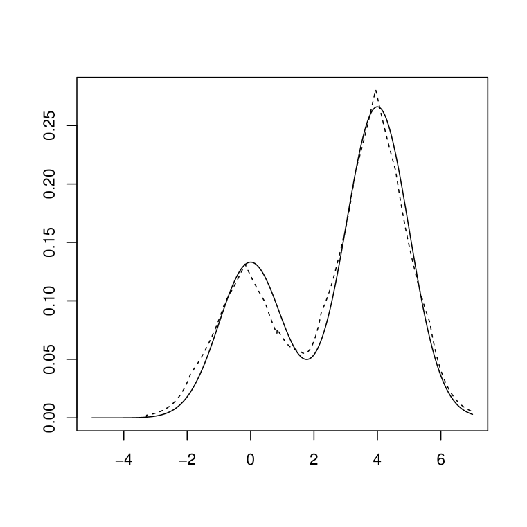
Figure 1: Left: plot of the true density of $(1/3)\mathcal{N}(0,1)+(2/3)\mathcal{N}(4,1)$ (solid line) and its log-concave estimator $\widehat{g}_{n}$ (dotted line). Right: plot of the density of $\mathcal{N}(0,1)$ and its zero-symmetric log-concave MLE $\widehat{f}_{n}$. The MLE was based on $n=500$ independent data drawn from the mixture density $(1/3)\mathcal{N}(0,1)+(2/3)\mathcal{N}(4,1)$.

5 Testing and clustering

Bordes et al. (2006), Hunter et al. (2007) and Butucea and Vandekerkhove (2014) propose three different ways of estimating the mixture parameters $\pi^{0},u^{0}_{1}$ and $u^{0}_{2}$. As we are interested here in $\sqrt{n}$-consistent estimators of these parameters, we prefer the work by Hunter et al. (2007) and Butucea and Vandekerkhove (2014). Also, due to some numerical instabilities encountered when computing the estimators proposed by Butucea and Vandekerkhove (2014), we adopt the approach of Hunter et al. (2007) which has been already implemented in R; one could either used the code posted at http://www.stat.psu.edu/~dhunter/code or the function in the mixtools package. The latter option was kindly brought to the attention of the first author by David Hunter in a private communication.

Once the estimates $\widecheck{\pi}_{n}$, $\widecheck{u}_{1,n}$ and $\widecheck{u}_{2,n}$ of $\pi^{0}$, $u^{0}_{1}$ and $u^{0}_{2}$ are computed, we maximize

$$f^{+}\mapsto\frac{1}{n}\sum_{i=1}^{n}\log\left(\widecheck{\pi}_{n}f^{+}(Z_{2i-1})+(1-\widecheck{\pi}_{n})f^{+}(Z_{2i})\right)$$

where $f^{+}=2f1_{[0,\infty)}$, $Z_{2i-1}=|X_{i}-\widecheck{u}_{1,n}|$ and $Z_{2i}=|X_{i}-\widecheck{u}_{2,n}|$ for $i=1,\ldots,n$. This is equivalent to maximizing (5), which we have shown to admit a maximizer. Since the log-likelihood is not concave and it is not clear how to maximize it directly, we will appeal to the EM algorithm (Dempster et al., 1977). Although we are fixing the parameters $\pi,u_{1}$, and $u_{2}$ we may still introduce the standard-in-mixture-models complete data of $(X_{i},\Delta_{i})$, where $\Delta_{i}\sim$ Bernoulli$(\pi)$ and $X_{i}|\left\{\Delta_{i}=1\right\}\sim f^{0}(\cdot-\widecheck{u}_{1,n})$ and $X_{i}|\left\{\Delta_{i}=0\right\}\sim f^{0}(\cdot-\widecheck{u}_{2,n})$. An iteration of the EM algorithm in this setup is then, given an estimate $\hat{f}^{+,(r)}_{n}$, to compute

$$\hat{f}^{+,(r+1)}_{n}:=\operatorname{argmax}_{f^{+}}\sum_{i=1}^{n}\left\{\hat{p}^{(r)}_{n,i}\log f^{+}(Z_{2i-1})+(1-\hat{p}^{(r)}_{n,i})\log f^{+}(Z_{2i})\right\}$$ (10)

where the argmax is over log-concave densities on $[0,\infty)$ with mode at $0$, and

$$\widehat{p}^{(r)}_{n,i}=\frac{\widecheck{\pi}_{n}\widehat{f}^{+,(r)}(Z_{2i-1})}{\widecheck{\pi}_{n}\widehat{f}^{+,(r)}(Z_{2i-1})+(1-\widecheck{\pi}_{n})\widehat{f}^{+,(r)}(Z_{2i})}$$

is the conditional expectation of $\Delta_{i}$ given $X_{i}$. To initialize the EM algorithm, we start with the density of a centered Gaussian distribution with variance equal to the estimate given in formula (11) of Hunter et al. (2007) for the true variance of the zero-symmetric component, that is $\frac{1}{n}\sum_{i=1}^{n}(X_{i}-\bar{X}_{n})^{2}-\widecheck{\pi}_{n}(1-\widecheck{\pi}_{n})(\widecheck{u}_{2,n}-\widecheck{u}_{1,n})^{2},$ or $1$ if this estimate is negative (this may occur for moderate sample sizes). The argmax in (10) can be computed by the R package logcondens.mode.

5.1 Testing the absence of mixing

Recall that the mixing model we consider in this paper is given by

$$g^{0}=\pi^{0}f^{0}(\cdot-u^{0}_{1})+(1-\pi^{0})f^{0}(\cdot-u^{0}_{2})$$

with $f^{0}$ a log-concave zero-symmetric density on $\mathbb{R}$, $\pi^{0}\notin\{0,1/2,1\}$ and $u^{0}_{1}<u^{0}_{2}$. We now use our log-concave MLE to test for the absence of mixing, i.e. to test for the null hypothesis that $u_{1}^{0}=u_{2}^{0}$, against the alternative that $u_{1}^{0}\neq u_{2}^{0}$ and $\pi^{0}\neq 1/2$ under the assumption that $f^{0}$ is zero-symmetric and log-concave.

To test for mixing we consider the likelihood ratio statistic. Under the null hypothesis, we take the estimator of the true density to be equal to the log-concave MLE which is symmetric around the median of the data. If $\widehat{g}_{n}^{0}$ denotes this estimator, then our test statistic is given by

$$\Lambda_{n}=\frac{\prod_{i=1}^{n}\widehat{g}_{n}(X_{i})}{\prod_{i=1}^{n}\widehat{g}_{n}^{0}(X_{i})}.$$ (11)

The null hypothesis is then rejected when $\Lambda_{n}$ is too large. We use the null hypothesis estimator to find critical values; that is, we bootstrap from the symmetric log-concave estimator $\widehat{g}^{0}_{n}$. The critical values of $\Lambda_{n}$ are then computed in the usual way: based on the bootstrapped samples from $\widehat{g}_{n}^{0}$, we compute the estimators of the mixing probability and mixture locations and the corresponding MLE $\widehat{g}_{n}$. The order statistics of the bootstrapped values of the likelihood ratio are then obtained to compute upper empirical quantiles of a given order. We also compare our test for mixing (hereafter referred to as the LR test) to the following procedures:

• the naive symmetric bootstrap (NSBS): we re-sample with replacement $n$ random variables $Z^{*}_{1},\ldots,Z^{*}_{n}$ from $\{\pm|X_{1}-\widehat{m}_{n}|,\ldots,\pm|X_{n}-\widehat{m}_{n}|\}$ with $\widehat{m}_{n}$ the median of $X_{1},\ldots,X_{n}$ and set $X^{*}_{i}=\widehat{m}_{n}+Z^{*}_{i},i=1,\ldots,n$. Then, the bootstrapped estimators of the location mixture of Hunter et al. (2007), $u^{*}_{1}$ and $u^{*}_{2}$, are computed based on $Y^{*}_{i},i=1,\ldots,n$. We repeat this procedure $B$ times and compute the empirical $(1-\alpha)$-quantile of the distribution of $u^{*}_{2}-u^{*}_{1}$. The null hypothesis is rejected if the observed $\widecheck{u}_{2,n}-\widecheck{u}_{1,n}$ is larger than this quantile.

• the naive symmetric bootstrap based on symmetric kernel density estimation (NSBSKDE): the method is similar to the one described above except that a standard kernel density estimator is fitted to $\widehat{m}_{n}\pm|X_{i}-\widehat{m}_{n}|$ and $X^{*}_{1},\ldots,X^{*}_{n}$ are now drawn from the fitted estimator at each bootstrap iteration.

• the likelihood ratio based on symmetric kernel density estimation (LRSKDE): two kernel density estimators are computed, one under the full model, that is, based on $X_{1},\ldots,X_{n}$, and one under the null model, that is, based on $\widehat{m}_{n}\pm|X_{i}-\widehat{m}_{n}|$. The likelihood ratio of these estimators is then computed. Bootstrap samples are obtained by simulation from the kernel estimator under the null hypothesis and then the empirical $(1-\alpha)$-quantile of the likelihood ratio is thereby computed. The null hypothesis is rejected if the observed likelihood ratio is larger that this quantile.

Note that the NSBS provides a comparison procedure not based on density estimation of the components. In assessing the power, we take the true zero-symmetric component $f^{0}$ to be one of the following distributions: (1) a standard Gaussian, (2) a double exponential, and (3) a uniform on $[-1,1]$, Also, we take the true parameters to be $\pi^{0}\in\{0.20,0.40\}$ and $(u^{0}_{1},u^{0}_{2})\in\{(0,0),(0,1),(0,3)\}$. We give the estimated probability of rejecting the null hypothesis based on $R=500$ replications with $B=49$ bootstrap samples in Table 1, for $n=250$. The simulation results show the LR and LRSKDE tests are both outperforming the NSBS and NSBSKDE with power nearly equal or equal to $1$ for the well-separated mixtures. However, all the considered tests seem to have a level larger than the specified level $\alpha=0.1$ for the uniform distribution. Further simulations, which we do not report here, show that this improves when the sample size is increased to $n=500$. Note that the mixtures with mixture probability $\pi^{0}=.4$ are more difficult to distinguish than those with $\pi^{0}=.2$. This is to be expected as the former mixtures are close to being symmetric around the mid-point $(u^{0}_{1}+u^{0}_{2})/2$.

It would be interesting to know whether the level of our testing procedure based on the bootstrapped likelihood ratio test equals the theoretical level. The problem is however far from being trivial. Deriving the asymptotic level for example would require establishing the limit distribution of our statistic under the null hypothesis and also showing that it admits a continuous cumulative distribution function. Establishing such results requires a thorough study of the global asymptotics of the log-concave MLE. As this is outside the scope of this paper, the question remains open.

Distribution	$\boldsymbol{\pi^{0}}$		$0$	$1$	$3$
$\mathcal{N}(0,1)$	$.2$	LR	$0.11$	$0.15$	$1.00$
		NSBS	$0.06$	$0.07$	$0.34$
		NSBSKDE	$0.07$	$0.08$	$0.40$
		LRSKDE	$0.11$	$0.11$	$1.00$
	$.4$	LR	*	$0.14$	$0.86$
		NSBS	*	$0.05$	$0.28$
		NSBSKDE	*	$0.08$	$0.26$
		LRSKDE	*	$0.11$	$0.87$
$\mathcal{L}(1)$	$.2$	LR	$0.11$	$0.22$	$0.99$
		NSBS	$0.11$	$0.01$	$0.01$
		NSBSKDE	$0.13$	$0.11$	$0.02$
		LRSKDE	$0.12$	$0.19$	$0.98$
	$.4$	LR	*	$0.14$	$0.89$
		NSBS	*	$0.08$	$0.12$
		NSBSKDE	*	$0.08$	$0.03$
		LRSKDE	*	$0.18$	$0.86$
$\mathcal{U}[-1,1]$	$.2$	LR	$0.19$	$0.92$	$1.00$
		NSBS	$0.11$	$0.07$	$0.16$
		NSBSKDE	$0.11$	$0.08$	$0.14$
		LRSKDE	$0.25$	$0.99$	$1.00$
	$.4$	LR	*	$0.60$	$1.00$
		NSBS	*	$0.09$	$0.78$
		NSBSKDE	*	$0.07$	$0.75$
		LRSKDE	*	$0.54$	$1.00$

Table 1: Values of the bootstrapped power for LR, NSBS, NSBSKDE and LRSKDE tests when the true density is $\pi^{0}f^{0}(\cdot-u^{0}_{1})+(1-\pi^{0})f^{0}(\cdot-u^{0}_{2})$, where $u^{0}_{1}=0$, $u^{0}_{2}-u^{0}_{1}\in\{0,1,3\}$, $\pi^{0}\in\{0.2,0.4\}$, and $f^{0}$ is one of the zero-symmetric log-concave densities shown in the first column. The nominal level is $\alpha=0.1$. The sample size is $n=250$, the number of bootstraps and the number of replications were taken to be $B=49$ and $R=500$, respectively. The common value of the power under $H_{0}$ is replaced by “*”.

	G	HG	SLC	KDE
$\mathcal{N}(0,1)$	$163\,(0.44)$	$170\,(0.30)$	$170\,(0.30)$	182 (0.88)
$\mathcal{L}(1)$	$223\,(0.64)$	$173\,(0.32)$	$174\,(0.28)$	154 (0.82)
$\mathcal{U}(-1,1)$	$144\,(0.15)$	$66\,(0.11)$	$55\,(0.10)$	105 (0.28)

Table 2: Comparison of the four different clustering methods given by the column labels, see text for more details. The reported numbers are the average number of misclassifications out of $n=500$ samples over $R=5000$ replications under each of the three log-concave densities in the left column. Here $u^{0}_{2}-u^{0}_{1}=1$ and $\pi^{0}=.2$. The numbers in parentheses are the corresponding standard errors.

5.2 Gaussian versus symmetric log-concave clustering

We now consider the problem of clustering, i.e., of assigning to each observation in a dataset a label without being given any “training” labels. We will assume that the data can be clustered into two groups, which we will do by by fitting the two-component mixture (2) and assigning a label to an observation $X$ based on whether our estimate of the posterior probability

$$\frac{\pi^{0}f^{0}(X-u^{0}_{1})}{\pi^{0}f^{0}(X-u^{0}_{1})+(1-\pi^{0})f(X-u^{0}_{2})}$$ (12)

is greater than $1/2$ or not.

We fit the mixture three different ways. In the first basic approach, labeled “G”, we maximize the likelihood (5) under the assumption that the component $f$ is a normal density. We use the EM algorithm to maximize the likelihood. Our next two approaches both use the method of Hunter et al. (2007) to estimate the mixture components $u^{0}_{1},u^{0}_{2}$, and $\pi^{0}$. Then we either fit the components using a Gaussian density (denoted “HG”), with variance estimate also given by Hunter et al. (2007), or we use the symmetric log-concave density estimator (denoted “SLC”) for the components. The fourth approach is based on the estimators of Hunter et al. (2007) and the kernel density estimator based on the inversion formula given in (9) by Bordes et al. (2006) where we truncate the infinite sum at some large integer $K>0$. Precisely, let $\bar{g}_{n}$ be a standard density estimator of the mixed density $g^{0}$. Then, the KDE of $f^{0}$ we use is given by $\max(1/2(\bar{f}_{n}(x)+\bar{f}(-x)),0)$ where

$$\bar{f}_{n}(x)=\sum_{k=0}^{K}\left(\frac{-\widecheck{\pi}_{n}}{1-\widecheck{\pi}_{n}}\right)^{k}\bar{g}_{n}\big{(}x+\widecheck{u}_{2,n}+k(\widecheck{u}_{2,n}-\widecheck{u}_{1,n})\big{)}.$$

We should note that this formula is only valid, when $\widecheck{\pi}_{n}<1/2$. Hence, $1-\widecheck{\pi}_{n}$ and $(\widecheck{u}_{2,n},\widecheck{u}_{1,n})$ should replace $\widecheck{\pi}_{n}$ and $(\widecheck{u}_{1,n},\widecheck{u}_{2,n})$ When $\widecheck{\pi}_{n}\geq 1/2$.

We record the average missclassification count when the true density is one of the densities in the left column of Table 2. In all cases the number of replications is $R=5000$, the sample size is $n=500$, $u^{0}_{2}-u^{0}_{1}=1$ and $\pi^{0}=.2$.

The performances of the four approaches were then compared, and the results are reported in Table 2. The KDE approach does clearly worse than the three other methods. The SLC outperforms HG by $16$% when the true density is $\mathcal{U}[-1,1]$. In the other cases, they perform similarly. All four methods define the two cluster regions by dividing the real line into two half-lines. The HG and SLC methods have the same mixture components so the shape of the component density estimates have to be dramatically different (e.g., uniform instead of normal) in order to noticeably change the results; note this somewhat deceiving outcome is not totally in contradiction with the finding of Cule et al. (2010) about the performance of their two-dimensional log-concave classifier applied to the Breast cancer data of Wisconsin; see Cule et al. (2010) for details. The authors found that the log-concave MLE reduces the percentage of misclassification from 10.36% obtained for the Gaussian estimate to only 8.43% for that particular data set. The posterior probabilities of cluster membership, which can be used as a measurement of uncertainty, can also differ noticeably between the HG method and our SLC method.

6 Data application

In this section, we apply our new estimation approach to two different datasets.

6.1 Old Faithful data

The data to which we first apply our estimation procedure are the times, in minutes, between eruptions of the Old Faithful geyser in Yellowstone National park. There are many forms of the Old Faithful data. As far as we know, the oldest version of the data was collected by S. Weisberg from R. Hutchinson in August 1978. The data we analyze were collected between August 1 and August 15, 1985 continuously, and are from Azzalini and Bowman (1990). The following explanation from Weisberg (2005) motivates interest in the data:

Old Faithful Geyser is an important tourist attraction, with up to several thousand people watching it erupt on pleasant summer days. The park service uses data like these to obtain a prediction equation for the time to the next eruption.

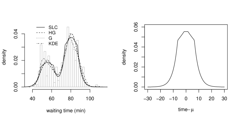
Figure 2: Time between eruptions of Old Faithful Geyser (min). The “SLC” and “HG” estimates both use the method of Hunter et al. (2007) to estimate the mixture parameters $u^{0}_{1},u^{0}_{2},$ and $\pi^{0}$. “SLC” then fits with symmetric log-concave components and “HG” fits with Gaussian components. The “G” estimate is the maximum likelihood estimate of a mixture model with two Gaussian components with equal variances. The ”KDE” is a standard kernel density estimator with an optimal bandwidth.

In Figure 2, we have two plots related to the Old Faithful data. The plot on the left depicts a descriptive histogram of the data with around $30$ bins (which is too many for optimal estimation) along with the plots of four mixture density estimates. The “SLC” (symmetric log-concave) estimate is the mixture model where $u^{0}_{1},u^{0}_{2}$ and $\pi^{0}$ are estimated using the method of Hunter et al. (2007), and then the components are estimated using our symmetric log-concave estimator. The “HG” (Hunter et al. and Gaussian components) estimate is given by again using the method of Hunter et al. (2007) to find estimates of the mixture parameters whereas the nonparametric components are taken to be Gaussian components (the same Gaussian density for both mixture components). The estimates for $u^{0}_{1},u^{0}_{2},$ and $\pi^{0}$ given by Hunter et al. (2007) are $55.5$, $80.5$, and $.33$, respectively. The “G” (Gaussian) estimate in the plot is based on simply using a Gaussian mixture model with two components with equal variances. Assuming equal variances forces the two components to be identical, which makes the model analogous to the others. In this case, we estimated $u^{0}_{1},u^{0}_{2},$ and $\pi^{0}$ by the EM algorithm (Dempster et al., 1977), with estimated values of $55.3$, $81.0$, and $.339$. The normal components are slightly more peaked than the log-concave ones, but the overall fit is fairly similar; in large part this is because the locations and weights are very similar. Finally, the ‘KDE’ is a standard kernel density estimator with an optimal bandwidth.

The plot on the right is that of the zero-symmetric log-concave component, centered at $0$, used in the mixture density. As expected from the known theoretical properties of this estimator, it has a flat interval about the origin, and is the exponential of a concave piecewise linear and zero-symmetric function.

6.2 Height data

We next examine $1766$ human height observations. We look at the heights of the population of Campora, a village in the south of Italy. This population is studied by the “Genetic Park of Cilento and Vallo di Dano Project” (Ciullo, 2009), which is interested in identifying geographically and genetically isolated populations. Such populations are of particular interest because in addition to “genetic homogeneity,” they have a “uniformity of diet, life style and environment.” These homogeneities are valuable in the study of genetic risk factors for complex pathologies such as “hypertension, diabetes, obesity, cancer, and neurodegenerative diseases,” by allowing for a “simplification of the complexity of genetic models” involved, because of the population’s homogeneity (Ciullo, 2009).

Colonna et al. (2007) provide evidence that this population is indeed genetically isolated. Because of this feature, the distribution of heights of this population is not necessarily the same as that of the global population at large, so estimating its distribution is of interest. Height data are often modeled as mixtures of two components, corresponding to the two sexes.

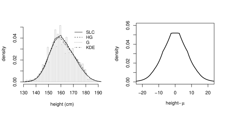
Figure 3: Height data of the population of Campora . The “SLC” and “HG” estimates both use the method of Hunter et al. (2007) to estimate the mixture parameters $u^{0}_{1},u^{0}_{2},$ and $\pi^{0}$. “SLC” then fits with symmetric log-concave components and “HG” fits with Gaussian components. The “G” estimate is the maximum likelihood estimate of a mixture model with two Gaussian components with equal variances. The ‘KDE’ is a standard kernel density estimator with an optimal bandwidth.

We present plots related to the height data in Figure 3. The height data do not exhibit multi-modality, but two-component mixtures still fit the data well. The three approaches that we consider fit similarly, but the log-concave components are able to capture a bit more asymmetry near to the mode.

The plot on the right includes the mixture component density (labeled “All”), in black. The data include the sex of each individual, so, using this extra information we can also estimate the true component densities separately: the zero-symmetric log-concave density estimate can be compared to the estimates of the density of the heights for either sex considered alone. Figure 4 shows the plots of the (descriptive) histograms of the heights for men and women and fitted standard kernel density estimators. The assumption of symmetry of the distribution of the heights for each of the genders seems to be reasonable to make. The observed proportion of women is $0.57$, whereas the observed medians of the heights for women and men were found to be $156.0$ and $168.7$, respectively. Using the estimation method of Hunter et al. (2007), we found $\widecheck{\pi}_{n}=0.72,\widecheck{u}_{1,n}=157.5,$ and $\widecheck{u}_{2,n}=170.5$. Here $\widecheck{\pi}_{n}$ and $\widecheck{u}_{1,n}$ correspond to the component for women.

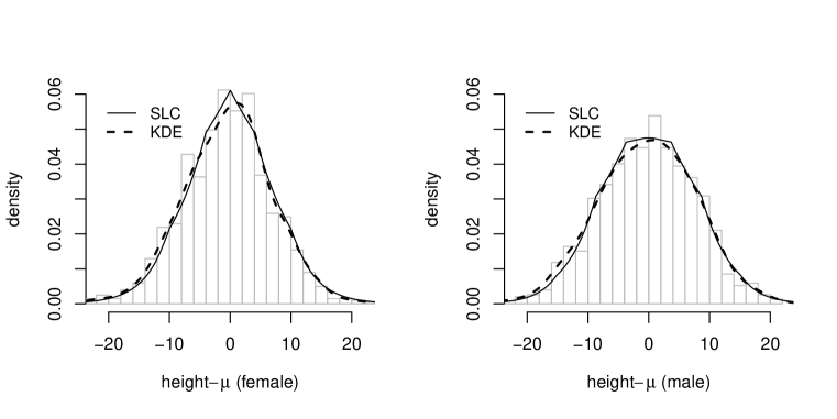
Figure 4: Descriptive histograms of the height data for women (left) and men (right) after centering around the median. The “SLC” is the log-concave MLE of the true density constrained to have mode at $0$. The “KDE” is a standard kernel density estimator with an optimal bandwidth.

The components estimated by using the labels for men and women differ from that using the mixture model without the labels especially towards the center. We believe that this is essentially due to the difference between the estimates of the mixture parameters $\pi^{0}$, $\mu_{1}^{0}$ and $\mu_{2}^{0}$ obtained by ignoring or using the information available about the gender. In the latter case, the locations are estimated by the respective medians. It does appear that the distributions of heights of men and women are somewhat different near those centers, with women having a more peaked density and men having a flatter one. Thus, in the mixture model, without using the labels, the component density estimate is somewhere in between the two shapes.

7 Conclusions

The goal in this paper is to make use of the log-concavity constraint to estimate the unknown density component in a semi-parametric location mixture model assuming that this unknown density is symmetric around the origin. The first motivation for choosing this approach is that many densities are log-concave. The second one is to build an estimation procedure that does not depend on a tuning parameter. Our log-concave MLE is computed by maximizing the log-likelihood function after estimating the mixture parameters using the approach of Hunter et al. (2007). The computation is easily implementable using the EM algorithm in combination with an active set algorithm already implemented in the R package logcondens.mode.

As already mentioned, our method is not advocated for heavy-tailed densities. In such cases, other shape constraints may be more appropriate, specifically, $s$-concavity, as studied in Koenker and Mizera (2010) and Doss and Wellner (2015). Unfortunately, the theory of estimators of $s$-concave densities is less developed than that of log-concave MLEs, which remains a barrier to using $s$-concavity in our current context.

Finally, Hunter et al. (2007) give sufficient conditions on the mixing probabilities and mixture locations for the model to be $3$-identifiable. In this case, the mixture parameters can still be computed using the method of Hunter et al. (2007), and the log-concave MLE can be computed as described in this paper. However, it is not immediate in that case whether the same proof approaches would still yield the same rate of convergence. Recently, Balabdaoui and Butucea (2014) proved that the number of components $k$, the mixture parameters and the unknown density are identifiable provided that the density is Pólya frequency (of infinite order) such that its expectation is equal to zero. For a precise definition of Pólya frequence functions, we refer to Schoenberg (1951). The obtained identifiability result can be used of course in the case of symmetry but it is certainly not a requirement. Note that imposing the log-concave constraint in this setting is natural since the class of Pólya frequency functions is a subset of the log-concave class as shown by Schoenberg (1951). One may argue that non-parametric classes such as symmetric densities or Pólya frequency functions with expectation equal to zero are not large enough. However, it seems that identifiability is hard to obtain if one allows for large classes.

Appendix A Supplement

Appendix B Appendix

B.1 Main Proofs

Proof of Proposition 2.1.  To show existence, we first start by proving that $\widehat{\psi}_{n}$ is necessarily a piecewise linear function that is flat in the neighborhood of zero. Let $\psi\in\mathcal{SC}$. Also, let $Z_{(1)}$ denote the first order statistic of the transformed data $Z_{i}$’s defined in Proposition 2.1. Consider $\bar{\psi}$ the unique concave function such that $\bar{\psi}(Z_{i})=\psi(Z_{i}),i=1,\ldots,2n$, $\bar{\psi}(0)=\bar{\psi}(Z_{(1)})$, $\bar{\psi}$ is piecewise linear between the points $Z_{i},i=1,\ldots,2n$, $\bar{\psi}(t)=-\infty$ for $t>Z_{(2n)}$ and $\psi(t)=\psi(-t)$ for $t\in\mathbb{R}$. Clearly, $\bar{\psi}\in\mathcal{SC}$ and admits the properties $\widecheck{\pi}_{n}e^{\bar{\psi}(X_{i}-\widecheck{u}_{1,n})}+(1-\widecheck{\pi}_{n})e^{\bar{\psi}(X_{i}-\widecheck{u}_{2,n})}=\widecheck{\pi}_{n}e^{\psi(X_{i}-\widecheck{u}_{1,n})}+(1-\widecheck{\pi}_{n})e^{\psi(X_{i}-\widecheck{u}_{2,n})}$ for $i=1,\ldots,n$ and $\bar{\psi}\leq\psi$. This implies that $\Phi_{n}(\bar{\psi})\geq\Phi_{n}(\psi)$ and the logarithm of the MLE has to be necessarily piecewise linear between the transformed data points $Z_{i}$ and $-Z_{i},i=1,\ldots,2n$ with a flat piece in the neighborhood of zero and support $[-Z_{(2n)},Z_{(2n)}]$. Further, if a maximizer $\widehat{f}_{n}=\exp(\widehat{\psi}_{n})$ exists then it has to be a density. This follows from the fact that $\widehat{\psi}_{n}+\epsilon\in\mathcal{SC}$ for all $\epsilon\in\mathbb{R}$, and

$$0=\lim_{\epsilon\to 0}\frac{\Phi_{n}(\widehat{\psi}_{n}+\epsilon)-\Phi_{n}(\widehat{\psi}_{n})}{\epsilon}=1-\int_{\mathbb{R}}\exp(\widehat{\psi}_{n}).$$

Given the results obtained above, a function $\psi\in\mathcal{SC}$ can be identified with the vector

$$\underline{\psi}\equiv\Big{(}\psi(X_{i}-\widecheck{u}_{1,n}),\psi(X_{i}-\widecheck{u}_{2,n})\Big{)}_{i=1}^{n}=\Big{(}\psi(Z_{2i-1}),\psi(Z_{2i})\Big{)}_{i=1}^{n}.$$

Let $\mathcal{SC}_{n}$ denote the set of such vectors. In this second part of the proof, we will show that the maximization problem admits a solution. It is clear that $\Phi_{n}$ is continuous on $\mathcal{SC}_{n}$. In the following, we will show that $\Phi_{n}$ is necessarily maximized on a compact set. To this aim, consider $\underline{\psi}^{(p)}$ to be a maximizing sequence, such that $\int\exp(\psi^{(p)}(t))dt=1$, and as $p\to\infty$

$$\max_{1\leq i\leq n}\big{|}\psi^{(p)}(Z_{(i)})\big{|}\to\infty,\ \textrm{and}\ \big{|}\psi^{(p)}(Z_{(i)})\big{|}\to l_{i}\in[-\infty,\infty],\ \textrm{for $1\leq i\leq n$}$$

where $Z_{(i)}$ denotes the $i$-th order statistic of $Z_{1},\ldots,Z_{2n}$.

For $1\leq i\leq n$ write $\psi^{(p)}_{i}:=\psi^{(p)}(Z_{(i)})$. Suppose that for all $i\in\{1,\ldots,n\}$

$$\lim_{p\to\infty}\psi^{(p)}_{i}<\infty.$$

This implies that there exists $j\in\{1,\ldots,n\}$ such that $\lim_{p\to\infty}\psi^{(p)}_{j}=-\infty$. If there exists $i\in\{1,\ldots,n\}$ such that $Z_{(j)}=\max(|X_{i}-\widecheck{u}_{1,n}|,|X_{i}-\widecheck{u}_{2,n}|)$ then

$$\lim_{p\to\infty}\log\left(\widecheck{\pi}_{n}\exp(\psi^{(p)}(|X_{i}-\widecheck{u}_{1,n}|))+(1-\widecheck{\pi}_{n})\exp(\psi^{(p)}(|X_{i}-\widecheck{u}_{2,n}|))\right) \leq \lim_{p\to\infty}\psi^{(p)}_{j}$$

$$= -\infty$$

implying that $\lim_{p\to\infty}\Phi_{n}(\psi^{(p)})=-\infty$ which is in contradiction with the definition of $\psi^{(p)}$.

Let us assume now that for any $j$ such that $\lim_{p\to\infty}\psi^{(p)}_{j}=-\infty$, there exists $i\in\{1,\ldots,n\}$ such that

$$Z_{(j)}=\min(|X_{i}-\widecheck{u}_{1,n}|,|X_{i}-\widecheck{u}_{2,n}|)\ \textrm{and}\ \lim_{n\to\infty}\psi^{(p)}(\max(|X_{i}-\widecheck{u}_{1,n}|,|X_{i}-\widecheck{u}_{2,n}|)>-\infty.$$ (13)

Suppose that $j=2n$ is the only integer for which this divergence is occurring. Let $i\in\{1,\ldots,n\}$ such that we have $Z_{(2n)}=\min(|X_{i}-\widecheck{u}_{1,n}|,|X_{i}-\widecheck{u}_{2,n}|)$. Without loss of generality, assume that $|X_{i}-\widecheck{u}_{1,n}|<|X_{i}-\widecheck{u}_{2,n}|$. Put

$$a^{(p)}=(1-\widecheck{\pi}_{n})\exp\left(\psi^{(p)}(|X_{i}-\widecheck{u}_{2,n}|)\right),\ \textrm{and}\ b^{(p)}=\psi^{(p)}_{2n-1}$$

and call $a$ and $b$ their respective limits as $p\to\infty$. Note that both $a$ and $b$ are in $\mathbb{R}$ by assumption. Consider now the function defined by

$$h(x) = \log\left(\widecheck{\pi}_{n}e^{x}+a\right)-2(Z_{(2n)}-Z_{(2n-1)})\frac{\exp(b)-\exp(x)}{b-x}$$

on $(-\infty,0]$. Put $\Delta_{2n-1}=Z_{(2n)}-Z_{(2n-1)}$. We have that

$$h^{\prime}(x)=\frac{\widecheck{\pi}_{n}\exp(x)}{\widecheck{\pi}_{n}\exp(x)+a}-\frac{2\Delta_{2n-1}}{b-x}\left(\frac{\exp(b)-\exp(x)}{b-x}-\exp(x)\right)$$

which has the same sign as

$$\widecheck{\pi}_{n}-2\Delta_{2n-1}\exp(b)\Big{(}\widecheck{\pi}_{n}\exp(x)+a\Big{)}\frac{1}{b-x}\left(\frac{\exp(-x)-\exp(-b)}{b-x}-\exp(-b)\right)$$

$$=\widecheck{\pi}_{n}-2\Delta_{2n-1}\exp(b)\Big{(}\widecheck{\pi}_{n}\exp(x)+a\Big{)}\frac{\exp(-x)-\exp(-b)}{(b-x)^{2}}\left(1-\frac{(b-x)\exp(-b)}{\exp(-x)-\exp(-b)}\right)$$

$$\to-\infty,\ \textrm{as $x\to-\infty$}.$$

This implies that as $p\to\infty$

$$\log\left(\widecheck{\pi}_{n}\exp(\psi^{(p)}(|X_{i}-\widecheck{u}_{1,n}|)+(1-\widecheck{\pi}_{n})\exp(\psi^{(p)}(|X_{i}-\widecheck{u}_{2,n}|))\right)-\int_{Z_{(2n-1)}}^{Z_{(2n)}}\exp(\psi^{(p)})(t)dt$$

must be decreasing, and hence bigger values of the log-likelihood are to be obtained if $\psi^{(p)}(Z_{(2n)})$ were not divergent. This implies that $\psi^{(p)}_{2n}$ cannot diverge to $-\infty$. The same reasoning can be applied if (13) is satisfied by other integers $k\in\{1,\ldots,2n-1\}$, and let $j$ be the smallest one. Let $i$ be such that $Z_{(j)}=\min(|X_{i}-\widecheck{u}_{1,n}|,|X_{i}-\widecheck{u}_{2,n}|)$. Note that $j>1$. Also, note that by definition of $j$ $\lim_{p\to\infty}\psi^{(p)}(Z_{(j-1)})>-\infty$. Thus, we obtain the same conclusion as before, that is, the term

$$\log\left(\widecheck{\pi}_{n}\exp(\psi^{(p)}(|X_{i}-\widecheck{u}_{1,n}|)+(1-\widecheck{\pi}_{n})\exp(\psi^{(p)}(|X_{i}-\widecheck{u}_{2,n}|))\right)-\int_{Z_{(j-1)}}^{Z_{(j)}}\exp(\psi^{(p)})(t)dt$$

can be increased (and hence the log-likelihood) if $\psi^{(p)}_{j}$ were not diverging to $-\infty$. By a recursive reasoning, we obtain the same conclusion about the remaining integers.

Now suppose that $\lim_{p\to\infty}\max_{1\leq i\leq n}\psi^{(p)}(Z_{(i)})=\infty$. Since $\psi^{(p)}$ is decreasing on $[0,\infty)$, $\max_{1\leq i\leq n}\psi^{(p)}(Z_{(i)})=\psi^{(p)}(Z_{(1)})\to\infty$ as $p\to\infty$. For $x\in[Z_{(1)},Z_{(2)}]$, we have

$$1 \geq \int_{Z_{(1)}}^{Z_{(2)}}\exp(\psi^{(p)}_{1})\exp\left(\frac{\psi^{(p)}_{2}-\psi^{(p)}_{1}}{Z_{(2)}-Z_{(1)}}(t-Z_{(1)})\right)dt$$

$$= \exp(\psi^{(p)}_{1})(Z_{(2)}-Z_{(1)})\frac{1-\exp(\psi^{(p)}_{1}-\psi^{(p)}_{2})}{\psi^{(p)}_{1}-\psi^{(p)}_{2}}$$

$$\geq \exp(\psi^{(p)}_{1})(Z_{(2)}-Z_{(1)})\frac{1}{\psi^{(p)}_{1}-\psi^{(p)}_{2}+1},$$

where the last inequality follows from the fact that $\frac{1-\exp(-t)}{t}\geq\frac{1}{t+1}$ on $[0,\infty)$. This implies that

$$\psi^{(p)}_{1}-\psi^{(p)}_{2}\geq\exp(\psi^{(p)}_{1})(Z_{(2)}-Z_{(1)})-1.$$

Thus

$$\psi^{(p)}_{1}+\psi^{(p)}_{2}=2\psi^{(p)}_{1}+\psi^{(p)}_{2}-\psi^{(p)}_{1}\leq 2\psi^{(p)}_{1}-\exp(\psi^{(p)}_{1})(Z_{(2)}-Z_{(1)})+1\to-\infty$$

as $p\to\infty$, and hence $\psi^{(p)}_{2}\leq(\psi^{(p)}_{1}+\psi^{(p)}_{2})/2\to-\infty$. Since a maximizer of $\Phi_{n}$ is necessarily constant on $[-\tau_{1},\tau_{1}]$ with $\tau_{1}$ the first kink point, here equal to $Z_{(1)}$, we can write

$$1=2\exp(\psi^{(p)}_{1})Z_{(1)}+\sum_{j=2}^{n}\int_{Z_{(j)}}^{Z_{(j+1)}}\exp(\psi^{(p)}(t))dt\geq 2\exp(\psi^{(p)}_{1})Z_{(1)}$$

But this implies using the results obtained above that $\exp(\psi^{(p)}_{1})\leq 1/(2Z_{(1)})$, which contradicts the assumption that $\psi^{(p)}_{1}\to\infty$. $\Box$

Proof of Proposition 2.2. This follows from arguments similar to those used in the proof of Theorem 2.2 of Dümbgen and Rufibach (2009). $\Box$

Proof of Proposition 2.3:  Using symmetry of $\widehat{f}_{n}$ and $\Delta$, and the definition of $\widehat{\mathbb{F}}_{n}$, the inequality in (7) can be re-written as

$$\int_{0}^{\infty}\Delta(x)d\widehat{\mathbb{F}}_{n}(x)\leq\int_{0}^{\infty}\Delta(x)\widehat{f}^{+}_{n}(x)dx,$$ (14)

with equality for $\Delta$ satisfying $\widehat{\psi}^{+}_{n}\pm\epsilon\Delta\in\mathcal{SC}$ for $\epsilon>0$ small enough. For $z\in[0,\infty)$, consider the concave perturbation function defined on $[0,\infty)$ as

$$\Delta_{z}(x) = -(x-z)_{+}$$

$$= \begin{cases}z-x\ \text{if $x\geq z$}\\ 0\ \ \text{otherwise}.\end{cases}$$

Using Fubini’s theorem, the inequality in (14) yields

$$Z_{(2n)}-z-\int_{z}^{Z_{(2n)}}\widehat{\mathbb{F}}_{n}(x)dx\geq Z_{(2n)}-z-\int_{z}^{Z_{(2n)}}\widehat{F}^{+}_{n}(x)dx.$$

This yields

$$\int_{0}^{z}\widehat{F}^{+}_{n}(x)dx\leq\int_{0}^{z}\widehat{\mathbb{F}}_{n}(x)dx+\int_{0}^{Z_{(2n)}}\widehat{F}^{+}_{n}(x)dx-\int_{0}^{Z_{(2n)}}\widehat{\mathbb{F}}_{n}(x)dx.$$

Since for $z=0$, the inequality in (14) becomes an equality ($\Delta_{0}$ is a straight line, and hence satisfies $\widehat{\psi}^{+}_{n}\pm\epsilon\Delta_{0}\in\mathcal{SC}$ for $\epsilon>0$ small enough), we have that

$$\int_{0}^{Z_{(2n)}}\widehat{\mathbb{F}}_{n}(x)dx=\int_{0}^{Z_{(2n)}}\widehat{F}^{+}_{n}(x)dx$$

from which follows the inequality part in (9). The equality part follows from noting that when $z$ is a knot of $\widehat{\psi}^{+}_{n}=\log(\widehat{f}^{+}_{n})$ we have $\widehat{\psi}^{+}_{n}\pm\epsilon\Delta_{z}\in\mathcal{SC}$ for $\epsilon>0$ small enough. $\Box$

Next we state and prove propositions and lemmas needed for the proofs of the theorems in Section 3, and then prove those theorems. We start by stating several propositions of the Glivenko-Cantelli type. To begin, let $\mathcal{C}$ be the class of convex and compact subsets (intervals) in $\mathbb{R}$. The following theorem of Bhattacharya and Ranga Rao (1976) will be an important component of the proof of Proposition B.1

Theorem B.1 (Theorem 1.11, page 22, Bhattacharya and Ranga Rao (1976))

Let $P$ be a probability measure on $\mathbb{R}$. Then, as $n\to\infty$

$$\sup_{C\in\mathcal{C}}|\mathbb{P}_{n}(C)-P(C)|\to 0$$

almost surely.

Proposition B.1

Fix $\alpha\in(0,1)$. Let $X_{1},\ldots,X_{n}$ be $n$ independent observations from the density $g^{0}=\widecheck{\pi}_{n}^{0}f^{0}(\cdot-u^{0}_{1})+(1-\widecheck{\pi}_{n}^{0})f^{0}(\cdot-u^{0}_{2})$, and $\widecheck{u}_{1,n}$ and $\widecheck{u}_{2,n}$ be any consistent estimators of $u^{0}_{1}$ and $u^{0}_{2}$. Write $\bar{u}_{n}=(\widecheck{u}_{1,n}+\widecheck{u}_{2,n})/2,\bar{u}^{0}=(u^{0}_{1}+u^{0}_{2})/2$ and let $\bar{N}=\sum_{i=1}^{n}1_{X_{i}\leq\bar{u}}$. Then, for any $\epsilon>0$, there exists $n_{0}$ such that

$$P\left(\min\bigg{\{}|C|:C\ \in\mathcal{C}\ \textrm{such that}\ \bar{N}^{-1}\sum_{i:X_{i}\leq\bar{u}_{n}}1_{\{X_{i}\in C\}}\geq\alpha\bigg{\}}\geq\frac{\alpha G(\bar{u}^{0})}{2\|g^{0}\|_{\infty}}\right)\geq 1-\epsilon$$

for all $n\geq n_{0}$.

Proof:  Let $\mathcal{C}$ denote the class of all convex and compact subsets in $\mathbb{R}$. Fix $\epsilon>0$. For $C\in\mathcal{C}$ we have that

$$\bar{N}^{-1}\sum_{i:X_{i}\leq\bar{u}}1_{\{X_{i}\in C\}}=\frac{\mathbb{P}_{n}(C\cap]-\infty,\bar{u}])}{\mathbb{G}_{n}(\bar{u})}=\frac{\mathbb{P}_{n}(C_{\bar{u}})}{\mathbb{G}_{n}(\bar{u})}.$$

where $C_{\bar{u}}=C\cap]-\infty,\bar{u}])$ is also compact and convex. To simplify notation, we write $C$ for $C_{\bar{u}_{n}})$, and $g$, $G$ and $P$ the true density, distribution function and associated measure respectively. Then

$$\frac{\mathbb{P}_{n}(C)}{\mathbb{G}_{n}(\bar{u}_{n})}-\frac{P(C)}{G(\bar{u}^{0})} = \frac{[\mathbb{P}_{n}(C)-P(C)]G(\bar{u}_{n})-P(C)[\mathbb{G}_{n}(\bar{u}_{n})-G(\bar{u}_{n})]}{\mathbb{G}_{n}(\bar{u}_{n})G(\bar{u}_{n})}$$

$$-\ \frac{P(C)[G(\bar{u}_{n})-G(\bar{u}^{0})]}{G(\bar{u}_{n})G(\bar{u}^{0})}.$$

Consistency of $\widecheck{u}_{1,n}$ and $\widecheck{u}_{2,n}$, the fact that the class $\{]-\infty,x]:x\in\mathbb{R}\}$ is Glivenko-Cantelli (see Example 2.5.4 of van der Vaart and Wellner (1996)) and continuity of $g$ imply that the event

$$\left\{G(\bar{u}_{n})\geq\frac{G(\bar{u}^{0})}{2},\mathbb{G}_{n}(\bar{u}_{n})\geq\frac{G(\bar{u}^{0})}{2},\max_{t\in[\bar{u}^{0}\wedge\bar{u}_{n},\bar{u}^{0}\vee\bar{u}_{n}]}g(t)\leq 2g(\bar{u}^{0})\right\}$$

occurs with probability converging to one. On the other hand, we have that

$$\left|\frac{\mathbb{P}_{n}(C)}{\mathbb{G}_{n}(\bar{u}_{n})}-\frac{P(C)}{G(\bar{u}^{0})}\right| \leq \frac{\sup_{C\in\mathcal{C}}|\mathbb{P}_{n}(C)-P(C)|+\sup_{x\in\mathbb{R}}|\mathbb{G}_{n}(x)-G(x)|}{\mathbb{G}_{n}(\bar{u}_{n})G(\bar{u}_{n})}$$

$$\ +\frac{|G(\bar{u}_{n})-G(\bar{u}^{0})|}{G(\bar{u}_{n})G(\bar{u}^{0})}$$

$$\leq \frac{\sup_{C\in\mathcal{C}}|\mathbb{P}_{n}(C)-P(C)|+\sup_{x\in\mathbb{R}}|\mathbb{G}_{n}(x)-G(x)|}{\mathbb{G}_{n}(\bar{u}_{n})G(\bar{u}_{n})}$$

$$\ +\frac{g(\xi)|\bar{u}_{n}-\bar{u}^{0}|}{G(\bar{u}_{n})G(\bar{u}^{0})},\ \ \textrm{for some $\xi\in[\bar{u}^{0}\wedge\bar{u}_{n},\bar{u}^{0}\vee\bar{u}_{n}]$}$$

$$\leq D\left(\sup_{C\in\mathcal{C}}|\mathbb{P}_{n}(C)-P(C)|+\sup_{x\in\mathbb{R}}|\mathbb{G}_{n}(x)-G(x)|+|\bar{u}_{n}-\bar{u}^{0}|\right)$$

probability increasing to one, where $D=4G(\bar{u}^{0})^{-2}\max(2g(\bar{u}^{0}),1)$. Using Theorem B.1, and again consistency of $\bar{u}_{n}$, we conclude that

$$\sup_{C\in\mathcal{C}}\left|\frac{\mathbb{P}_{n}(C)}{\mathbb{G}_{n}(\bar{u}_{n})}-\frac{P(C)}{G(\bar{u}^{0})}\right|\to 0\ \ \textrm{in probability as }n\to\infty.$$

In particular, this implies that for any fixed $\epsilon>0$ there exists $n_{0}$ such that

$$P\left(\frac{\mathbb{P}_{n}(C)}{\mathbb{G}_{n}(\bar{u}_{n})}\leq\frac{P(C)}{G(\bar{u}^{0})}+\frac{\alpha}{2}\ \textrm{for all $C\in\mathcal{C}$}\right)\geq 1-\epsilon.$$

Let us denote by $\mathcal{E}_{n,\alpha/2}$ the event $\left\{\frac{\mathbb{P}_{n}(C)}{\mathbb{G}_{n}(\bar{u}_{n})}\leq\frac{P(C)}{G(\bar{u}^{0})}+\frac{\alpha}{2}\ \textrm{for all $C\in\mathcal{C}$}\right\}$. Also, consider the subclass

$$\mathcal{C}_{\alpha/2}=\left\{C\in\mathcal{C}:\frac{P(C)}{G(\bar{u}^{0})}\geq\frac{\alpha}{2}\right\}.$$

Clearly, for any $C\in\mathcal{C}_{\alpha/2}$ we have that

$$|C|\geq\frac{\alpha G(\bar{u}^{0})}{2\|g\|_{\infty}}.$$

On the other hand,

$$\left\{\ C\in\mathcal{C}:\bar{N}^{-1}\sum_{i:X_{i}\leq\bar{u}_{n}}1_{\{X_{i}\in C\}}\geq\alpha\right\}=\left\{\ C\in\mathcal{C}:\frac{\mathbb{P}_{n}(C)}{\mathbb{G}_{n}(\bar{u}_{n})}\geq\alpha\ \textrm{for $C\in\mathcal{C}$}\right\}$$

$$=\left\{\left\{C\in\mathcal{C}:\frac{\mathbb{P}_{n}(C)}{\mathbb{G}_{n}(\bar{u}_{n})}\geq\alpha\right\}\cap\mathcal{E}_{n,\alpha/2}\right\}\ \cup\ \left\{\left\{C\in\mathcal{C}:\frac{\mathbb{P}_{n}(C)}{\mathbb{G}_{n}(\bar{u}_{n})}\geq\alpha\right\}\cap\mathcal{E}^{c}_{n,\alpha/2}\right\}$$

$$\subseteq\mathcal{C}_{\alpha/2}\ \cup\ \left\{\left\{C\in\mathcal{C}:\frac{\mathbb{P}_{n}(C)}{\mathbb{G}_{n}(\bar{u}_{n})}\geq\alpha\}\right\}\cap\mathcal{E}^{c}_{n,\alpha/2}\right\}$$

implying that for $n\geq n_{0}$

$$P\left(\min\big{\{}|C|:C\ \in\mathcal{C}\ \textrm{such that}\ \bar{N}^{-1}\sum_{i:X_{i}\leq\bar{u}_{n}}1_{\{X_{i}\in C\}}\geq\alpha\big{\}}<\frac{\alpha G(\bar{u}^{0})}{2\|g^{0}\|_{\infty}}\right)\leq\epsilon$$

completing the proof of the Proposition. $\Box$

Lemma B.1

Let $\psi\in\mathcal{SC}$, $a<b\ \in\mathbb{R}$ and $\lambda\in[0,1]$. If $p(t)=\lambda\exp(\psi(t-a))+(1-\lambda)\exp(\psi(t-b))$, then

$$\int_{\mathbb{R}}|\log(p(t))|p(t)dt<\infty.$$

Proof: Note that for $t\in\mathbb{R}$ we have that

$$|t-a|\leq|t-b|\Longleftrightarrow t\leq(a+b)/2.$$

Using the fact that the function $t\mapsto|\log(t)|t$ is increasing on $(0,e^{-1}]$ and that $\psi$ is decreasing on $[0,\infty)$, we have for $A$ taken to be larger than $(a+b)/2$,

$$\int_{A}^{\infty}\Big{|}\log(p(t))|p(t)dt \leq \int_{A}^{\infty}|\psi(t-a)|\exp(\psi(t-a))dt$$

$$< \infty$$

where the second inequality follows e.g. from Lemma 2 in Schuhmacher and Dümbgen (2010). By symmetry, the integral on $(-\infty,-A]$ is also finite. $\Box$

In the following, we introduce a condition that will be useful in proving consistency of our estimator.

The condition (C): We will say that an (ordered) pair $(f,h)=(e^{\psi},e^{\phi})$ of log-concave densities satisfy the condition $(C)$ if for all $d\in\mathbb{R}$,

$$\int_{0}^{\infty}\left|\phi(t+d)\right|f(t)dt<\infty.$$

Note that $h$ must have support $(-\infty,\infty)$.

Lemma B.2

Let $\psi_{0}$ and $\phi$ be elements of $\mathcal{SC}$. Let $a_{0}<b_{0}$ be real numbers and $\lambda_{0}\in[0,1]$. Let $(a_{k})$, $(b_{k})$, and $(\lambda_{k})$, for $k>0$, be sequences of real numbers converging to $a_{0},b_{0}$, and $\lambda_{0}$, respectively. Let

$$p_{k}(\cdot) =\lambda_{k}\exp(\psi_{0}(\cdot-a_{k}))+(1-\lambda_{k})\exp(\psi_{0}(\cdot-b_{k})),$$

$$p_{k,\phi}(\cdot) =p_{k}(\cdot)\star e^{\phi(\cdot)}=\lambda_{k}\exp(\psi_{0}(\cdot-a_{k}))\star e^{\phi(\cdot)}+(1-\lambda_{k})\exp(\psi_{0}(t-b_{k}))\star e^{\phi(\cdot)},$$

for $k=0,1,\ldots$. Let $e^{\psi_{0}}$ and $e^{\phi}$ satisfy condition $(C)$. Then

$$\int_{\mathbb{R}}\log\left(p_{k,\phi}(t)\right)p_{0}(t)\,dt\longrightarrow\int_{\mathbb{R}}\log\left(p_{0,\phi}(t)\right)p_{0}(t)\,dt$$ (15)

as $k\to\infty$.

Proof:  It is enough to show that for $k$ large, $|\log p_{k,\phi}|$ is bounded by a $p_{0}$-integrable function to apply the Lebesgue Dominated Convergence Theorem. Since $p_{k,\phi}$ is uniformly bounded above, to upper bound $|\log p_{k,\phi}|$ we need to lower bound $p_{k,\phi}$. Now,

$$p_{k,\phi}(x) =\int_{\mathbb{R}}p_{k}(y)e^{\phi(x-y)}\,dy\geq\int_{\alpha}^{\beta}\left(\min_{z\in[\alpha,\beta]}p_{k}(z)\right)e^{\phi(x-y)}\,dy$$ (16)

for any $\alpha$ and $\beta$. Taking $\alpha$ and $\beta$ to be in the interior of the support of $p_{0}$, we have that, for all $k$ large enough, $\min_{z\in[\alpha,\beta]}p_{k}(z)\geq c$ for some $c>0$. Now because $\phi$ is concave, if $x\geq A$ where $A$ is large enough, $\phi$ is decreasing on $[x-\beta,x-\alpha]$, i.e. ${\phi(x-y)}$ is increasing in $y$ for $y\in[\alpha,\beta]$, so that then $\phi(x-y)\geq\phi(x-\alpha)$. Taking $A$ large enough that $\phi(x-\alpha)<0$, so $|\phi(x-y)|\leq|\phi(x-\alpha)|$, we have that, for $k$ large, and $x>A$, (16) is bounded below by

$$c\int_{\alpha}^{\beta}e^{\phi(x-\alpha)}\,dy=(\beta-\alpha)ce^{\phi(x-\alpha)}.$$

Recall that if $d_{1}<d_{2}$, then

$$|t-d_{1}|\leq|t-d_{2}|\Longleftrightarrow t\leq(d_{1}+d_{2})/2.$$

Thus, taking $A>(a+b)/2$,

$$\int_{A}^{\infty}|\phi(x-\alpha)|p_{0}(x)\,dx\leq\int_{A}^{\infty}|\phi(x-\alpha)|e^{\psi_{0}(x-b_{0})}\,dx=\int_{A+b}^{\infty}|\phi(x-\alpha+b)|e^{\psi_{0}(x)}\,dx,$$

and this is less than infinity, by the condition $(C)$. Thus, for $x\geq A$ and $k$ large,

$$|\log p_{k,\phi}(x)|\leq|\log\left((\beta-\alpha)c\right)|+|\phi(x-\alpha)|,$$

so we have shown that $|\log p_{k,\phi}|$ is bounded by a function $p_{0}$-integrable on $[A,\infty)$. A similar argument shows it is bounded by a function integrable on $(-\infty,-A]$. Finally, since $p_{0,\phi}$ has support $(-\infty,\infty)$ (since $e^{\phi}$ has support $(-\infty,\infty)$ by the condition $(C)$),

$$\sup_{x\in[-A,A]}|\log p_{k,\phi}(x)|\leq\sup_{x\in[-A-\eta,A+\eta]}|\log p_{0}(x)|<\infty,$$

for all $k$ large enough that $\max(|a_{0}-a_{k}|,|b_{0}-b_{k}|)<\eta$ for some $\eta>0$. Thus for $k$ large we have shown that $|\log p_{k,\phi}|$ is bounded by a $p_{0}$-integrable function on $\mathbb{R}$, and $p_{k,\phi}(t)\to p_{0,\phi}(t)$ for all $t\in\mathbb{R}$, so (15) holds. $\Box$

Note that for any log-concave density $f=e^{\psi}$, if $\phi$ is a polynomial function, then $f$ and $e^{\phi}$ satisfy condition (C), since log-concave densities have finite moments of all orders. In particular, we may take $e^{\phi}$ to be any normal density, which we will do below in the proof of consistency. Theorem 3.1 will rely on the following two Glivenko-Cantelli propositions. As is standard, we say that a class of functions $\cal F$ is a $G$-Glivenko-Cantelli class if $\sup_{f\in\mathcal{F}}|{\mathbb{G}}_{n}(f)-G(f)|\to 0$ as $n\to\infty$ almost surely, where ${\mathbb{G}}_{n}$ is the empirical probability measure based on i.i.d. draws from $G$, and we write $\mu(f)=\int fd\mu$ for a function $f$ and a measure $\mu$ (as in e.g. van der Vaart and Wellner (1996) or van de Geer (2000)). (This is sometimes known as being strong Glivenko-Cantelli because the convergence is almost sure, rather than in probability (van der Vaart and Wellner, 2000).)

Proposition B.2

Let $M>0$ and $\mathcal{LC}_{M}$ be the class of log-concave functions bounded by $M$. For a fixed $b>0$, consider the class of functions

$$\mathcal{F}_{b}=\Big{\{}f:f=\log(\lambda h_{1}+(1-\lambda)h_{2}+b),\ h_{1},h_{2}\in\mathcal{LC}_{M},\ \lambda\in[0,1]\Big{\}}.$$

Then $\mathcal{F}_{b}$ is a Glivenko-Cantelli class for any probability measure $P$.

Proof:  Since all $f\in{\cal LC}_{M}$ are unimodal, ${\cal LC}_{M}\subset{\cal M}_{M}^{+}-{\cal M}_{M}^{+}$ where ${\cal M}_{M}^{+}:=\left\{f:0\leq f\leq M,f\mbox{ is nondecreasing}\right\}$. By Theorem 2.7.5 and Theorem 2.4.1 in van der Vaart and Wellner (1996), ${\cal M}_{M}^{+}$ is a (strong) $P$-Glivenko-Cantelli class for any $P$. By the Glivenko-Cantelli preservation Theorem 3 of van der Vaart and Wellner (2000), $\varphi({\cal M}_{M}^{+},{\cal M}_{M}^{+})$ is $P$-Glivenko-Cantelli, with $\varphi(x,y):=x-y$ here, so ${\cal LC}_{M}$ also is $P$-Glivenko-Cantelli, since it has an integrable envelope by construction. Now letting $\varphi(h_{1},h_{2},\lambda):=\log\left(\lambda h_{1}+(1-\lambda)h_{2}+b\right)$, another application of Theorem 3 of van der Vaart and Wellner (2000) yields that ${\cal F}_{b}=\varphi\left({\cal LC}_{M},{\cal LC}_{M},\left\{\lambda\mathbbm{1}_{(-\infty,\infty)}(x):\lambda\in[0,1]\right\}\right)$ is also Glivenko-Cantelli since each of the three argument classes are, as long as ${\cal F}_{b}$ has a $P$-integrable envelope. But this is immediate since $\log(b)\leq f\leq\log(M+b)$ for all $f\in{\cal F}_{b}$. $\Box$

We will also need a Glivenko-Cantelli result for the case $b=0$. In order for such a result to hold, we need to restrict attention to just logs of mixtures of a single density; despite the unboundedness of the functions involved, this will allow us to have an integrable envelope, at least for the true $P_{0}$.

Proposition B.3

Fix $\tilde{f}_{0}\in\mathcal{SLC}_{1}$, $\widecheck{\pi}_{n}\in[0,1]$, $a<b$ and let $p_{0}(x)=\widecheck{\pi}_{n}\tilde{f}_{0}(x-a)+(1-\widecheck{\pi}_{n})\tilde{f}_{0}(x-b),\ x\in\mathbb{R}$, and $P_{0}$ the corresponding probability measure. Let $q\in\mathcal{SLC}_{1}$ be such that $(\tilde{f}_{0},q)$ satisfy the Condition (C). Then the class of functions

$$\mathcal{H} =\Big{\{}\log\left(\lambda q(x-\alpha)+(1-\lambda)q(x-\beta)\right):$$

$$\hskip 28.45274pt\ \alpha\in\big{[}a-r,a+r\big{]},\beta\in\big{[}b-r,b+r\big{]},\lambda\in[0,1]\Big{\}}$$

for any fixed $r>0$ is $P_{0}$-Glivenko-Cantelli.

Proof:  Without loss of generality, we take $r=1$ in this proof. For any $c\in\mathbb{R}$ let $\mathcal{P}_{c}:=\left\{q(\cdot-z):z\in[c-1,c+1]\right\}$. Then the classes ${\cal P}_{a}$ and ${\cal P}_{b}$ are both contained in $\mathcal{LC}_{M}$ with $M=\sup_{x}q(x)$, and in the proof of Proposition B.2 we showed that $\mathcal{LC}_{M}$ is $P$-Glivenko-Cantelli for any $P$. Let $T(h_{1},h_{2},\lambda):=\log\left(\lambda h_{1}+(1-\lambda)h_{2}\right)$ and let $I_{0,1}:=\left\{\lambda\mathbbm{1}_{(-\infty,\infty)}(x):\lambda\in[0,1]\right\}$. Then by Theorem 3 of van der Vaart and Wellner (2000), the class $T\left(\mathcal{P}_{a},\mathcal{P}_{b},I_{0,1}\right)$ is $P_{0}$-Glivenko-Cantelli as long as it has a $P_{0}$-integrable envelope, which is what we will show now.

Let $c_{+}\in\mathbb{R}$ be such that $\log q(x-(b+1))<0$ if $x>c_{+}$. Then for any $h\in\mathcal{H}$, $h(x)\leq 0$ for $x>c_{+}$ by the unimodality of $q$. Note $q(x-\alpha)\geq q(x-(a-1))$ for $x\geq a+1\geq\alpha\geq a-1$ and $q(x-\beta)\geq q(x-(b-1))$ if $x\geq b+1\geq\beta\geq b-1$. Thus, for $x>(b+1)\vee c_{+}$, $h\in\mathcal{H}$ satisfies

$$0\geq h(x) \geq\log\left(\lambda q(x-(a-1))+(1-\lambda)q(x-(b-1))\right)$$

$$\geq\log q(x-(a-1)),$$ (17)

since $b>a$. A similar argument shows for $x<(a-1)\wedge c_{-}$ for some $c_{-}\in\mathbb{R}$, that $0\geq h(x)\geq\log q(x-(b+1))$. By the assumption that Condition $(C)$ holds for $(\tilde{f}_{0},q)$, it is immediate that $\log q(\cdot-(a-1))$ and $\log q(\cdot-(b+1))$ are $p_{0}$-integrable. All $h\in\mathcal{H}$ are uniformly bounded on $[(a-1)\wedge c_{-},(b+1)\vee c_{+}]$, since the support of $p_{0,\varphi}$ is $\mathbb{R}$, since $p_{0,\varphi}$ is unimodal, and since the range of $\alpha$ and $\beta$ in the definition of $\cal H$ is bounded. Thus $\mathcal{H}$ has a $P_{0}$-integrable envelope and so we are done. $\Box$

Theorem B.2

Let $\widehat{g}_{n}$ denote again the MLE of the mixed density. Then, for a given $\epsilon>0$ there exist an integer $n_{0}>0$ and $D>0$ depending on $\epsilon$ such that

$$P\left(\|\widehat{g}_{n}\|_{\infty}\leq D\right)\geq 1-\epsilon.$$

for all $n\geq n_{0}$.

Proof:  Fix $\epsilon>0$. Recall that if $a<b$, then for $t\in\mathbb{R}$

$$|t-a|\leq|t-b|\Longleftrightarrow t\leq(a+b)/2.$$

Write $\bar{u}=(\widecheck{u}_{1,n}+\widecheck{u}_{2,n})/2$. Using the symmetry of $\widehat{\psi}_{n}$ and the fact that it is decreasing on $[0,\infty)$, it follows that

$$\Phi_{n}(\log(\widehat{g}_{n}))\leq\frac{1}{n}\sum_{i:X_{i}\leq\bar{u}}\widehat{\psi}_{n}(X_{i}-\widecheck{u}_{1,n})+\frac{1}{n}\sum_{i:X_{i}>\bar{u}}\widehat{\psi}_{n}(X_{i}-\widecheck{u}_{2,n})-1.$$ (18)

Without loss of generality, we can assume that $\{X_{1},X_{2},\ldots,X_{\bar{N}}\}=\{X_{i}:X_{i}\leq\bar{u}\}$ and that $\psi_{n}(X_{1}-\widecheck{u}_{1,n})<\ldots<\widehat{\psi}_{n}(X_{\bar{N}}-\widecheck{u}_{1,n})$,and that

$$\max_{i:X_{i}>\bar{u}}\widehat{\psi}_{n}(X_{i}-\widecheck{u}_{2,n})\leq\max_{i:X_{i}\leq\bar{u}}\widehat{\psi}_{n}(X_{i}-\widecheck{u}_{1,n})$$

otherwise the same reasoning above has to be applied to the second term of the right side of the inequality in (18). In the following, let

$$M_{n}=\widehat{\psi}_{n}(X_{n}-\widecheck{u}_{1,n})$$

the largest value taken by $\widehat{\psi}_{n}(X_{i}-\widecheck{u}_{1,n})$ and $\widehat{\psi}_{n}(X_{i}-\widecheck{u}_{2,n})$ for $i=1,\ldots,n$.

Following the notation of Schuhmacher and Dümbgen (2010) in the proof of their Lemma 4, let $k=\lfloor\bar{N}\alpha\rfloor$ for some fixed $\alpha\in(0,1]$, $\mathcal{C}_{k}$ the convex hull of the set $\{X_{i}-\widecheck{u}_{1,n},i\geq k\}$ and $m=\widehat{\psi}_{n}(X_{k}-\widecheck{u}_{1,n})$. Also, let

$$\eta=\frac{\alpha G(\bar{u}^{0})}{2\|g^{0}\|_{\infty}}.$$

In the sequel, $\mathcal{C}_{k}+\widecheck{u}_{1,n}=\{t+\widecheck{u}_{1,n}:t\in\mathcal{C}_{k}\}$. Note that $\mathcal{C}_{k}+\widecheck{u}_{1,n}$ is convex and compact such that

$$\sum_{i:X_{i}\leq\bar{u}}1_{\{X_{i}\in\mathcal{C}_{k}+\widecheck{u}_{1,n}\}}=\sum_{i=1}^{\bar{N}}1_{\{X_{i}\in\mathcal{C}_{k}+\widecheck{u}_{1,n}\}}=\bar{N}-k+1\geq\bar{N}(1-\alpha).$$

By taking $1-\alpha$ in place of $\alpha$ in Proposition B.1, we can find an integer $n_{0}>0$ such that for $n\geq n_{0}$.

$$P\left(|C_{k}|\geq\eta\right)\geq 1-\epsilon/5.$$ (19)

Consider the event

$$\Big{\{}M_{n}>B_{0}:=\max(\log(1/\eta)+1,0)\Big{\}}.$$ (20)

Using the same argument as in Schuhmacher and Dümbgen (2010), we can write

$$1=\int_{\mathbb{R}}e^{\widehat{\psi}_{n}(t)}dt \geq \int_{\mathcal{C}_{k}}e^{\widehat{\psi}_{n}(t)}dt$$ (21)

$$\geq e^{m}|\mathcal{C}_{k}|$$

using monotonicity of $\widehat{\psi}_{n}$ on the convex set $\mathcal{C}_{k}$. By (20). Hence,

$$\Big{\{}M_{n}>B_{0},|\mathcal{C}_{k}|>\eta\Big{\}}\subset\{M_{n}>m+1\}.$$ (22)

Indeed, this follows from the fact that

$$e^{M_{n}-1} > 1/\eta,\ \ \ \textrm{by (\ref{IneqMn})}$$

$$> 1/|\mathcal{C}_{k}|$$

$$\geq e^{m}\ \textrm{by (\ref{Ineqm})}.$$

Also, on the event on the right side of (22), we have for $t$ such that $t\in\mathcal{C}_{k}+\widecheck{u}_{1,n}$

$$\widehat{\psi}_{n}\left(X_{n}-\widecheck{u}_{1,n}+\frac{t-X_{n}}{M_{n}-m}\right) \geq \frac{1}{M_{n}-m}\widehat{\psi}_{n}(t-\widecheck{u}_{1,n})+\frac{M_{n}-m-1}{M_{n}-m}\widehat{\psi}_{n}(X_{n}-\widecheck{u}_{1,n})$$

$$\geq \frac{m}{M_{n}-m}+\frac{M_{n}(M_{n}-m-1)}{M_{n}-m}=M_{n}-1.$$

Thus,

$$\textrm{Leb}(x\in\mathbb{R}:\widehat{\psi}_{n}(x)\geq M_{n}-1)\geq\textrm{Leb}\left(\frac{M_{n}-m-1}{M_{n}-m}(X_{n}-\widecheck{u}_{1,n})+\frac{1}{M_{n}-m}\mathcal{C}_{k}\right)=\frac{|\mathcal{C}_{k}|}{M_{n}-m},$$

and hence

$$1=\int_{\mathbb{R}}e^{\widehat{\psi}_{n}(t)}dt\geq\frac{e^{M_{n}-1}|\mathcal{C}_{k}|}{M_{n}-m}$$

Hence, the event on the right side of (22) is included in

$$\Big{\{}m\leq M_{n}-e^{M_{n}-1}|\mathcal{C}_{k}|<M_{n}-e^{M_{n}-1}\eta\Big{\}}.$$

Let $B_{1}>0$ be large enough so that $B_{1}>B_{0}$, $B_{1}-e^{B_{1}-1}\eta<-e^{B_{1}-1}\eta/2$ and $x\mapsto x-e^{x-1}\eta/2$ is decreasing on $[B_{1},\infty)$, and consider the event

$$\Big{\{}M_{n}>B_{1},|\mathcal{C}_{k}|>\eta\Big{\}}.$$

Then, this event is included in

$$\Big{\{}m\leq-e^{M_{n}-1}\eta/2\Big{\}}$$

and occurrence of the latter implies in turn that

$$\Phi_{n}(\log(\widehat{g}_{n}))\leq\frac{1}{n}\left[(\lfloor\alpha\bar{N}\rfloor-1)M_{n}-(\bar{N}-\lfloor\alpha\bar{N}\rfloor+1)\frac{1}{2}e^{M_{n}-1}\eta+\frac{n-\bar{N}}{n}M_{n}\right],$$

and consequently

$$\Phi_{n}(\log(\widehat{g}_{n}))\leq\left(1-(1-\alpha)\frac{\bar{N}}{n}\right)M_{n}-\frac{(1-\alpha)\bar{N}}{2n}e^{M_{n}-1}\eta.$$

Using similar arguments as in the proof of our Proposition B.1, we can increase $n_{0}$ to ensure that for $n\geq n_{0}$

$$P\left(\frac{\bar{N}}{n}\geq\frac{G^{0}(\bar{u}^{0})}{2}\right)\geq 1-\epsilon/5.$$

Hence, occurrence of the event

$$\Bigg{\{}M_{n}>B_{1},|C_{k}|>\eta,\frac{\bar{N}}{n}\geq\frac{G^{0}(\bar{u}^{0})}{2}\Bigg{\}}.$$

implies that

$$\Phi_{n}(\log(\widehat{g}_{n}))\leq\left(1-(1-\alpha)\frac{G^{0}(\bar{u}^{0})}{2}\right)M_{n}-\frac{(1-\alpha)G^{0}(\bar{u}^{0})}{4}\eta e^{M_{n}-1}$$ (23)

Next, if we take $e^{w}=\varphi_{\sigma}$ the density of standard Normal random variable. Then,

$$\Phi_{n}(\log(\widehat{g}_{n})) \geq \Phi_{n}\left(\widecheck{\pi}_{n}e^{w(\cdot-\widecheck{u}_{1,n})}+(1-\widecheck{\pi}_{n})e^{w(\cdot-\widecheck{u}_{2,n})}\right)$$

$$= \int_{\mathbb{R}}\log\left(\widecheck{\pi}_{n}e^{w(x-\widecheck{u}_{1,n})}+(1-\widecheck{\pi}_{n})e^{w(x-\widecheck{u}_{2,n})}\right)d(\mathbb{G}_{n}(x)-G^{0}(x))$$

$$\ +\int_{\mathbb{R}}\log\left(\widecheck{\pi}_{n}e^{w(x-\widecheck{u}_{1,n})}+(1-\widecheck{\pi}_{n})e^{w(x-\widecheck{u}_{2,n})}\right)g^{0}(x)dx-1.$$

For $\eta>0$ small enough, it follows from consistency of $\widecheck{u}_{1,n},\widecheck{u}_{2,n}$ and $\widecheck{\pi}_{n}$ that the event

$$\mathcal{E}^{0}=\Big{\{}|\widecheck{\pi}_{n}-\widecheck{\pi}_{n}^{0}|\leq\eta/2,|\widecheck{u}_{1,n}-u^{0}_{1}|\leq\eta/2,|\widecheck{u}_{2,n}-u^{0}_{2}|\leq\eta/2\Big{\}}$$

occurs with probability greater than $1-\epsilon/5$ for $n\geq n_{0}$ (at the cost of increasing the previous $n_{0}$). By Proposition B.3, since $(f^{0},e^{w})$ certainly satisfy Condition $(C)$, this implies that the event

$$\mathcal{E}_{\text{emp}}=\Bigg{\{}\left|\int_{\mathbb{R}}\log\left(\widecheck{\pi}_{n}e^{w(x-\widecheck{u}_{1,n})}+(1-\widecheck{\pi}_{n})e^{w(x-\widecheck{u}_{2,n})}\right)d(\mathbb{G}_{n}(x)-G^{0}(x))\right|\leq\frac{1}{2}\Bigg{\}}$$

occurs with probability greater than $1-\epsilon/5$ for $n\geq n_{0}$. Also, there exists a constant $D>0$ (depending on $\epsilon$) such that the event

$$\mathcal{E}_{KL}=\Bigg{\{}\left|\int_{\mathbb{R}}\log\left(\widecheck{\pi}_{n}e^{w(x-\widecheck{u}_{1,n})}+(1-\widecheck{\pi}_{n})e^{w(x-\widecheck{u}_{2,n})}\right)g^{0}(x)dx\right|\leq D\Bigg{\}}$$

with probability greater than $1-\epsilon/5$. Indeed, note that $\widecheck{\pi}_{n}e^{w(x-\widecheck{u}_{1,n})}+(1-\widecheck{\pi}_{n})e^{w(x-\widecheck{u}_{2,n})}\leq 1$ for all $x\in\mathbb{R}$ so that

$$\left|\int_{\mathbb{R}}\log\left(\widecheck{\pi}_{n}e^{w(x-\widecheck{u}_{1,n})}+(1-\widecheck{\pi}_{n})e^{w(x-\widecheck{u}_{2,n})}\right)g^{0}(x)dx\right|$$

$$=-\int_{\mathbb{R}}\log\left(\widecheck{\pi}_{n}e^{w(x-\widecheck{u}_{1,n})}+(1-\widecheck{\pi}_{n})e^{w(x-\widecheck{u}_{2,n})}\right)g^{0}(x)dx.$$

Using this fact and concavity of the logarithm, it follows that

$$0 \leq -\int_{\mathbb{R}}\log\left(\widecheck{\pi}_{n}e^{w(x-\widecheck{u}_{1,n})}+(1-\widecheck{\pi}_{n})e^{w(x-\widecheck{u}_{2,n})}\right)g^{0}(x)dx$$

$$\leq \frac{1}{2}\int_{\mathbb{R}}\left(\widecheck{\pi}_{n}(x-\widecheck{u}_{1,n})^{2}+(1-\widecheck{\pi}_{n})(x-\widecheck{u}_{2,n})^{2}\right)g^{0}(x)dx$$

$$< \infty$$

since log-concave densities have finite moments of any order. Put $L=-3/2-D$, and let $B_{2}>B_{1}$ such that

$$\left(1-(1-\alpha)\frac{G(\bar{u}^{0})}{2}\right)B_{2}-\frac{(1-\alpha)G(\bar{u}^{0})}{4}\eta e^{B_{2}-1}<L$$

and the function $x\mapsto\left(1-(1-\alpha)\frac{G(\bar{u}^{0})}{2}\right)x-\frac{(1-\alpha)G(\bar{u}^{0})}{4}\eta e^{x-1}$ is decreasing on $[B_{2},\infty)$. By the choice of $B_{2}$ above, we see that

$$\mathcal{E}_{\cap}=\Bigg{\{}M_{n}>B_{2},|C_{k}|>\eta,\frac{\bar{N}}{n}\geq\frac{G^{0}(\bar{u}^{0})}{2}\ \Bigg{\}}\cap\mathcal{E}^{0}\cap\mathcal{E}_{\text{emp}}\cap\mathcal{E}_{KL}=\emptyset$$

Hence,

$$P\Big{(}\|\widehat{g}_{n}\|_{\infty}>B_{2}\Big{)}=P(M_{n}>B_{2})=P(M_{n}>B_{2},\mathcal{E}_{\cap}^{c})\leq P(\mathcal{E}_{\cap}^{c})\leq\epsilon.$$

Note that $B_{2}$ depends on $\epsilon$ through $L$. $\Box$

To establish the first consistency result, note by the definition of $\widehat{g}_{n}$ we have that for any density $\tilde{g}$ of the form

$$\tilde{g}=\widecheck{\pi}_{n}f(\cdot-\widecheck{u}_{1,n})+(1-\widecheck{\pi}_{n})f(\cdot-\widecheck{u}_{2,n}).$$

for $f\in\mathcal{SLC}_{1}$ that

$$0\leq\int\log\widehat{g}_{n}\,d{\mathbb{G}}_{n}-\int\log\tilde{g}\,d{\mathbb{G}}_{n}\leq\int\log(\widehat{g}_{n}+b)\,d{\mathbb{G}}_{n}-\int\log\tilde{g}\,d{\mathbb{G}}_{n}.$$

Now let $b>0$, and $G^{0}$ be the cdf of the true mixed density $g^{0}$. As first established by Pal et al. (2007) in their Lemma 1, the inequality above yields

$$\begin{split}2H^{2}(\widehat{g}_{n},g^{0})&\leq\epsilon(b)+\int_{\mathbb{R}}\log(\widehat{g}_{n}(t)+b)d(\mathbb{G}_{n}(t)-G^{0}(t))\\ &\quad+\ \int_{\mathbb{R}}\log(g^{0}(t)+b)dG^{0}(t)-\int_{\mathbb{R}}\log(\tilde{g}(t))dG^{0}(t)\\ &\quad-\int_{\mathbb{R}}\log(\tilde{g}(t))d(\mathbb{G}_{n}(t)-G^{0}(t))\end{split}$$ (24)

where $H(p,q)$ denotes the Hellinger distance and

$$\epsilon(b)=2\int_{\mathbb{R}}\sqrt{\frac{b}{b+g^{0}(t)}}dG^{0}(t).$$

The main idea behind introducing the small positive quantity $b$ is to avoid integration issues due to the fact that $\log(\widehat{g}_{n})=-\infty$ outside a certain interval. In the problem of estimating a log-concave density, the empirical term on the right side of the previous inequality was shown to converge to zero using the fact that the maximum value of the log-concave MLE stays bounded in $n$, see Theorem 3.2 of Pal et al. (2007) and Lemma 4 in Schuhmacher and Dümbgen (2010) for a generalization of the same result in the multivariate setting. This property of the MLE was then combined with the fact that a level set of a bounded unimodal function is convex and compact. This cannot be claimed anymore if we replace a unimodal function by a mixture of two unimodal functions, not even when those functions are log-concave. For this reason, we shall use instead the Glivenko-Cantelli results proved above.

In our proof, the natural choice for $\tilde{g}$ would be

$$\widecheck{g}_{n}=\widecheck{\pi}_{n}f^{0}(\cdot-\widecheck{u}_{1,n})+(1-\widecheck{\pi}_{n})f^{0}(\cdot-\widecheck{u}_{2,n}),$$ (25)

but this is problematic. For instance $\int\log\widecheck{g}_{n}d{\mathbb{G}}_{n}$ can be $-\infty$ for arbitrarily large $n$ if $g^{0}$ has compact support. This might occur when the smallest/ largest order statistic is very close to the left/right end of the support if $f^{0}$ and $\widecheck{u}_{1,n}$/$\widecheck{u}_{2,n}$ is smaller/larger than $\widecheck{u}_{1,n}^{0}$/$u^{0}_{2}$. But even if $g^{0}$ does not have compact support, if it does have too large a slope (e.g., it approximates having compact support by dropping towards $0$ very quickly at some point), then $\int\log\widecheck{g}_{n}\,dG^{0}$ can still be infinite. Thus, we consider the surrogate density function

$$\widecheck{g}_{n,h}=\widecheck{\pi}_{n}f^{0}_{h}(\cdot-\widecheck{u}_{1,n})+(1-\widecheck{\pi}_{n})f^{0}_{h}(\cdot-\widecheck{u}_{2,n})$$ (26)

where $f^{0}_{h}=f^{0}\star\phi_{h}$, the convolution of $f^{0}$ and the density of centered normal with standard deviation $h>0$. This choice alleviates the above-mentioned problems; the risk of having a divergent log-likelihood is now excluded since $f_{h}^{0}$, the component density of $\widecheck{g}_{n,h}$, is supported on $\mathbb{R}$. Note that $f^{0}_{h}$ is a log-concave density by preservation of log-concavity under convolution (Ibragimov, 1956), and is symmetric.

Proof of Theorem 3.1:  The proof starts from the inequality in (24) with $\widecheck{g}_{n,h}$ (defined in (26)) as $\tilde{g}$. Theorem B.2 says that $\|\widehat{g}_{n}\|_{\infty}$ is $O_{p}(1)$, so $\|\widehat{f}_{n}\|_{\infty}$ is also $O_{p}(1)$, meaning that for any $\epsilon>0$, there is an $M$ such that $\widehat{f}_{n}$ lies in $\mathcal{LC}_{M}$ (the class of log-concave functions bounded by $M$) with probability $1-\epsilon$. Thus, we can apply Proposition B.2 to conclude that

$$\left|\int_{\mathbb{R}}\log\left(\widehat{g}_{n}(t)+b\right)d\left({\mathbb{G}}_{n}(t)-G^{0}(t)\right)\right|\leq\sup_{p\in\mathcal{F}_{b}}\left|\int_{\mathbb{R}}p\;d\left({\mathbb{G}}_{n}-G^{0}\right)\right|<\epsilon$$

with probability $1-\epsilon$ for $n$ large. Now, let us write

$$g^{0}_{h}(t)=\widecheck{\pi}_{n}^{0}f^{0}(\cdot-u^{0}_{1})\star\phi_{h}+(1-\widecheck{\pi}_{n}^{0})f^{0}(\cdot-u^{0}_{2})\star\phi_{h}$$

where $\phi_{h}$ is the density of a $N(0,h^{2})$ random variable. It then follows from Lemma B.2 that as $n\to\infty$,

$$\int_{\mathbb{R}}\log(\widecheck{g}_{n,h})dG^{0}\to_{p}\int_{\mathbb{R}}\log(g_{h}^{0})dG^{0}.$$

Now, since $\int_{\mathbb{R}}|\log(g^{0})|dG^{0}<\infty$, by Lemma 3.4 of Seregin and Wellner (2010),

$$\epsilon(b)+\int\left(\log(g^{0}(t)+b)-\log(g_{h}^{0}(t))\right)dG^{0}(t)\to\int\left(\log(g^{0})-\log(g_{h}^{0})\right)dG^{0}$$ (27)

as $b\searrow 0$, by the dominated convergence theorem. Now, for $|t|$ large enough, $g_{h}^{0}(t)\geq g^{0}(t)$, so $|\log g_{h}^{0}(t)|\leq|\log g^{0}(t)|$, and by Seregin and Wellner (2010), as was just mentioned, the latter is $g^{0}$-integrable, so that the right side of (27) converges to $0$ as $h\searrow 0$. Thus, for $\epsilon>0$, we can take $b$ and $h$ small enough that

$$\left|\epsilon(b)+\int_{\mathbb{R}}\log(g^{0}(t)+b)dG^{0}(t)-\int_{\mathbb{R}}\log(\widecheck{g}_{n,h})dG^{0}\right|<\epsilon$$

with high probability for $n$ large enough. Now, with $h$ fixed, by Proposition B.3,

$$\left|\int_{\mathbb{R}}\log(\widecheck{g}_{n,h})d({\mathbb{G}}_{n}-G^{0})\right|\leq\sup_{p\in\mathcal{H}}\left|\int_{\mathbb{R}}p\;d({\mathbb{G}}_{n}-G^{0})\right|<\epsilon$$

with high probability for $n$ large, where $\cal H$ is defined as in Proposition B.3 with $q$ taken as $f_{h}^{0}$ and $p_{0}$ taken as $g^{0}$; the proof of Lemma B.2 shows that since $(f^{0},\phi_{h})$ satisfy Condition $(C)$ then $\log f^{0}_{h}$ is $g_{0}$-integrable, and in fact for any $d\in\mathbb{R}$, $\log f^{0}_{h}(\cdot-d)$ is $g_{0}$-integrable (and so is $f_{0}$-integrable, so $(f^{0},f^{0}_{h})$ satisfy the condition $(C)$ as needed for Proposition B.3). Thus by (24) we are done. $\Box$

Proof of Corollary 3.1.  Recall the definition of $\widecheck{g}_{n}$ from (25), as well as the well-known fact that for any two densities $p_{1}$ and $p_{2}$,

$$\frac{1}{4}\left(\int_{\mathbb{R}}\big{|}p_{1}(t)-p_{2}(t)\big{|}dt\right)^{2}\leq H^{2}(p_{1},p_{2})\leq\int_{\mathbb{R}}\big{|}p_{1}(t)-p_{2}(t)\big{|}dt.$$ (28)

Assuming that $\widecheck{\pi}_{n}^{0}<1/2$ implies by consistency that $\widecheck{\pi}_{n}<1/2$ with increasing probability. Hence, the inversion formula (9) in Bordes et al. (2006) yields

$$\int_{\mathbb{R}}\big{|}\widehat{f}_{n}(t)-f^{0}(t)\big{|}dt \leq \frac{1}{1-\widecheck{\pi}_{n}}\sum_{k=0}^{\infty}\left(\frac{\widecheck{\pi}_{n}}{1-\widecheck{\pi}_{n}}\right)^{k}\int_{\mathbb{R}}\big{|}\widehat{g}_{n}(t)-\widecheck{g}_{n}(t)\big{|}dt$$ (29)

$$= \frac{1}{1-2\widecheck{\pi}_{n}}\int_{\mathbb{R}}\big{|}\widehat{g}_{n}(t)-\widecheck{g}_{n}(t)\big{|}dt.$$

From the first inequality in (28) and Theorem 3.1 above, it follows that

$$\int_{\mathbb{R}}|\widehat{g}_{n}(t)-g^{0}(t)|dt=o_{p}(1)$$

which in turn implies that

$$\int_{\mathbb{R}}|\widehat{g}_{n}(t)-\widecheck{g}_{n}(t)|dt=o_{p}(1).$$

Indeed,

$$\int_{\mathbb{R}}|\widehat{g}_{n}(t)-\widecheck{g}_{n}(t)|dt\leq\int_{\mathbb{R}}|\widehat{g}_{n}(t)-g^{0}(t)|dt+\int_{\mathbb{R}}|g^{0}(t)-\widecheck{g}_{n}(t)|dt$$

with

$$\int_{\mathbb{R}}|g^{0}(t)-\widecheck{g}_{n}(t)|dt \leq 2|\widecheck{\pi}_{n}-\widecheck{\pi}_{n}^{0}|+\int_{\mathbb{R}}|f^{0}(t-\widecheck{u}_{1,n})-f^{0}(t-u^{0}_{1})|dt$$

$$\ +\int_{\mathbb{R}}|f^{0}(t-\widecheck{u}_{2,n})-f^{0}(t-u^{0}_{2})|dt$$

$$= o_{p}(1)$$

by consistency of $\widecheck{\pi}_{n}$, $\widecheck{u}_{1,n}$ and $\widecheck{u}_{2,n}$ and Lemma B.3. It follows now from (29) and the inequalities in (28) that

$$H(\widehat{f}_{n},f^{0})=o_{p}(1),\ \textrm{and}\ \int_{\mathbb{R}}|\widehat{f}_{n}(t)-f^{0}(t)|dt=o_{p}(1).$$

Note that convergence of the MLE $\widehat{f}_{n}$ in probability to 0 in the $L_{1}$ distance implies its weak convergence to $f^{0}$ with increasing probability. Hence, for any arbitrary sequence $(n^{\prime})$ we can extract a further subsequence $(n^{\prime\prime})$ such that $\widehat{f}_{n^{\prime\prime}}$ converges weakly to $f^{0}$ almost surely. Hence, the assertion (c) in Proposition 2 of Cule and Samworth (2010) holds almost surely for $f_{n}=\widehat{f}_{n^{\prime\prime}}$ and $f=f^{0}$, and the remaining claims of our lemma now follow since $(n^{\prime})$ was chosen arbitrarily. $\Box$

Next, we prove the results in Section 4.

Proof of Proposition 4.1:  It follows from the recent result of Doss and Wellner (2015); see their Theorem 4.1 for $s=0$, that the classes

$$\Bigg{\{}f(\cdot-a),\ f\in\mathcal{SLC},\ f(0)\in[1/M,M],\ a\in[a_{0}-\delta,a_{0}+\delta]\Bigg{\}}$$

and

$$\Bigg{\{}f(\cdot-b),\ f\in\mathcal{SLC},\ f(0)\in[1/M,M],\ b\in[b_{0}-\delta,b_{0}+\delta]\Bigg{\}}$$

have both the same bracketing entropy $\log(N)\lesssim 1/\sqrt{\epsilon}$, where $\lesssim$ means that the term on the left side is smaller or equal than the term on the right side up to a positive constant. Let $\{\epsilon,\ldots,K\epsilon\}$, a $\epsilon$-net for $[0,1]$, where $K=\lfloor 1/\epsilon\rfloor+1$. For $i\in\{1,\ldots,N\}$, let $[l_{i},u_{i}]$ and $[l^{\prime}_{i},u^{\prime}_{i}]$ an $\epsilon$-bracket for the first and second class respectively. Note that since the brackets are in the Hellinger sense, we have that $u_{i}\geq l_{i}\geq 0$ and $u^{\prime}_{i}\geq l^{\prime}_{i}\geq 0$. Now, there exist $i\in\{1,\ldots,N\}$ and $j\in\{1,\ldots,K\}$ such that

$$\underline{g}\equiv(j-1)\epsilon l_{i}+(1-j\epsilon)l^{\prime}_{i}\leq\lambda f(x-a)+(1-\lambda)f(x-b)\leq\overline{g}\equiv j\epsilon u_{i}+(1-(j-1)\epsilon)u^{\prime}_{i}$$

with

$$H^{2}\left(\underline{g},\overline{g}\right)$$

$$=\frac{1}{2}\int_{\mathbb{R}}\left\{\Big{(}j\epsilon u_{i}(t)+(1-(j-1)\epsilon)u^{\prime}_{i}(t)\Big{)}^{1/2}-\Big{(}(j-1)\epsilon l_{i}(t)+(1-j\epsilon)l^{\prime}_{i}(t)\Big{)}^{1/2}\right\}^{2}dt$$

$$\leq 2H^{2}\Big{(}(j-1)\epsilon l_{i}+(1-(j-1)\epsilon)u^{\prime}_{i},j\epsilon u_{i}+(1-(j-1)\epsilon)u^{\prime}_{i}\Big{)}$$

$$\ +2H^{2}\Big{(}(1-j\epsilon)l^{\prime}_{i}+(j-1)\epsilon l_{i},(1-(j-1)\epsilon)u^{\prime}_{i}+(j-1)\epsilon l_{i}\Big{)}$$

$$\leq 2H^{2}\Big{(}(j-1)\epsilon l_{i},j\epsilon u_{i}\Big{)}+2H^{2}\Big{(}(1-j\epsilon)l^{\prime}_{i},(1-(j-1)\epsilon)u^{\prime}_{i}\Big{)},\ \textrm{by Lemma \ref{Hellinger}}$$

$$\leq 4(j-1)\epsilon\ H^{2}(l_{i},u_{i})+4\Big{(}\sqrt{j}-\sqrt{j-1}\Big{)}^{2}\epsilon$$

$$+\ 4(1-j\epsilon)\ H^{2}(l^{\prime}_{i},u^{\prime}_{i})+4\Big{(}\sqrt{1-(j-1)\epsilon}-\sqrt{1-j\epsilon}\Big{)}^{2},\ \textrm{applying again Lemma \ref{Hellinger}}.$$

Using the fact that $0\leq j\epsilon\leq 1$ and $1-(j-1)\epsilon\geq\epsilon$ for all $j\in\{1,\ldots,K\}$, we conclude from the preceding calculations that

$$H^{2}\left(\underline{g},\overline{g}\right)\leq 4H^{2}(l_{i},u_{i})+4H^{2}(l^{\prime}_{i},u^{\prime}_{i})+8\epsilon\lesssim\epsilon.$$

The proof is complete by noting that

$$\log N_{[\ ]}(\epsilon,\mathcal{G},H) \leq \log K+\log N\leq\log\left(\frac{1}{\epsilon}+1\right)+\log N$$

$$\leq \frac{1}{\sqrt{\epsilon}}+\log N\lesssim\frac{1}{\sqrt{\epsilon}}$$

using the fact that $\log(x+1)\leq\sqrt{x}$ for all $x\in[0,\infty)$. $\Box$

To prepare for the proof of Theorem 4.1, we recall that $\widecheck{\pi}_{n}$, $\widecheck{u}_{1,n}$ and $\widecheck{u}_{2,n}$ are estimates of $\widecheck{\pi}_{n}^{0}$, $u^{0}_{1}$ and $u^{0}_{2}$ respectively, that are converging at the rate $1/\sqrt{n}$. Recall also that $\widecheck{g}_{n}=\widecheck{\pi}_{n}f^{0}(\cdot-\widecheck{u}_{1,n})+(1-\widecheck{\pi}_{n})f^{0}(\cdot-\widecheck{u}_{2,n})$, and that $\widehat{g}_{n}=\widecheck{\pi}_{n}\widehat{f}_{n}(\cdot-\widecheck{u}_{1,n})+(1-\widecheck{\pi}_{n})\widehat{f}_{n}(\cdot-\widecheck{u}_{2,n})$, where $\widehat{f}_{n}$ is the log-concave MLE. As done in van der Vaart and Wellner (1996) (page 326, Section 3.4), we consider the criterion function

$$r_{n,g}=\log\frac{g+\tilde{g}_{n}}{2\tilde{g}_{n}}$$

for $g$ and

$$\tilde{g}_{n}=\widecheck{\pi}_{n}\tilde{f}_{n}(\cdot-\widecheck{u}_{1,n})+(1-\widecheck{\pi}_{n})\tilde{f}_{n}(\cdot-\widecheck{u}_{2,n})$$

with $\tilde{f}_{n}\in\mathcal{SCG}_{1}$ to be constructed. Note that

$$r_{n,\tilde{g}_{n}}=0,\textrm{and}\ \mathbb{P}_{n}r_{n,\widehat{g}_{n}}\geq\frac{1}{2}{\mathbb{P}}_{n}\log\frac{\widehat{g}_{n}}{\tilde{g}_{n}}\geq 0$$ (30)

where the second claim follows from the definition of the MLE $\widehat{g}_{n}$ and concavity of the logarithm.

Consider now the class of functions

$$\mathcal{R}_{n,\eta} = \Big{\{}r_{n,g}-r_{n,\tilde{g}_{n}}:g\in\mathcal{G},H(g,\tilde{g}_{n})<\eta\Big{\}}=\Big{\{}r_{n,g}:g\in\mathcal{G},H(g,\tilde{g}_{n})<\eta\Big{\}}.$$

If $P^{0}$ denotes again the true probability measure associated with $g^{0}$, let

$$\mathbb{G}_{n}(r_{n,g})=\sqrt{n}\left(\mathbb{P}_{n}-P^{0}\right)r_{n,g}=\sqrt{n}\left(\frac{1}{n}\sum_{i=1}^{n}r_{n,g}(X_{i})-\int r_{n,g}(x)dP^{0}(x)\right)$$

and denote

$$\|\mathbb{G}_{n}\|_{\mathcal{R}_{n,\eta}}=\sup_{g\in\mathcal{R}_{n,\eta}}\left|\mathbb{G}_{n}(r_{n,g})\right|.$$

Finally, define

$$\tilde{J}_{[\ ]}(\delta,\mathcal{G},H)=\int_{0}^{\delta}\sqrt{1+\log N_{[\ ]}(\epsilon,\mathcal{G},H)}d\epsilon.$$

Theorem 3.4.4 of van der Vaart and Wellner (1996) gives sufficient conditions to obtain control on $\|\mathbb{G}_{n}\|_{\mathcal{R}_{n,\eta}}$ in the mean. This control will involve the bracketing entropy bound obtained for the class $\mathcal{G}$. One of the crucial conditions to be fulfilled is that the sequence of densities $\tilde{g}_{n}$ need to be chosen such that $\tilde{g}_{n}$ approximates the truth $g^{0}$ and

$$\frac{g^{0}}{\tilde{g}_{n}}\leq M$$ (31)

for some $M>0$. Note that the reason we cannot choose $\tilde{g}_{n}=g^{0}$ is that in this problem maximization of the log-likelihood involve the random variables $\widecheck{\pi}_{n},\widecheck{u}_{1,n}$ and $\widecheck{u}_{2,n}$, hence it is not at all straightforward to compare the values taken by the criterion at $\widehat{g}_{n}$ and $g^{0}$. As will be shown in Proposition B.4, we will exhibit an approximating sequence $\tilde{g}_{n}$ that will satisfy the condition in (31) with increasing probability. Based on this proposition, we give now the proof of Theorem 4.1 along the same lines of the proof of Theorem 3.25 in van der Vaart and Wellner (1996); see page 290.

Proof of Theorem 4.1.  Fix $\epsilon>0$. Let $\tilde{g}_{n}$ be the approximating sequence of Proposition B.4, and consider the shells

$$S_{j,n}=\Big{\{}g:2^{j-1}<n^{2/5}H(g,\tilde{g}_{n})\leq 2^{j}\Big{\}}$$

for integers $j\geq 1$. Fix an integer $J\geq 1$, and consider the event

$$\Big{\{}n^{2/5}H(\widehat{g}_{n},\tilde{g}_{n})>2^{J}\Big{\}}.$$

Occurrence of this event implies that $\widehat{g}_{n}$ belongs to some $S_{j,n}$ with $j\geq J$. But our remark in (30) implies that

$$\sup_{g\in S_{j,n}}\left(\mathbb{P}_{n}r_{n,g}-\mathbb{P}_{n}r_{n,\tilde{g}_{n}}\right)=\sup_{g\in S_{j,n}}\mathbb{P}_{n}r_{n,g}\geq 0.$$

Thus, for any $\delta>0$ and $M>0$ we can write

$$P\left(n^{2/5}H(\widehat{g}_{n},\tilde{g}_{n})>2^{J}\right) = P\left(n^{2/5}H(\widehat{g}_{n},\tilde{g}_{n})>2^{J},g^{0}\leq M\tilde{g}_{n}\right)+P\left(g^{0}>M\tilde{g}_{n}\right)$$

$$= \sum_{j\geq J,2^{j}\leq n^{2/5}\eta}P\left(\sup_{g\in S_{j,n}}\left(\mathbb{P}_{n}r_{n,g}-\mathbb{P}_{n}r_{n,\tilde{g}_{n}}\right)\geq 0,g^{0}\leq M\tilde{g}_{n}\right)$$

$$+\ P\left(H(\widehat{g}_{n},\tilde{g}_{n})\geq\delta/2\right)+P\left(g^{0}>M\tilde{g}_{n}\right).$$

By Proposition B.4, for any $\eta>0$ and $M$ large enough the second and third terms are bounded by $\epsilon/2$. Now, using Theorem 3.4.4 of van der Vaart and Wellner (1996), we have

$$P^{0}(r_{n,g}-r_{n,\tilde{g}_{n}})\lesssim-H^{2}(g,\tilde{g}_{n})$$ (32)

for all densities $g$ such that $H(g,\tilde{g}_{n})\geq 32MH(\tilde{g}_{n},g^{0})$, and

$$E_{P^{0}}\|\mathbb{G}_{n}\|_{\mathcal{R}_{n,\eta}}\lesssim\tilde{J}_{[\ ]}(\eta,\mathcal{G},H)\left(1+\frac{\tilde{J}_{[\ ]}(\eta,\mathcal{G},H)}{\eta^{2}\sqrt{n}}\right).$$ (33)

From Proposition 4.1, we know that there exists a constant $K>0$ (not depending on $n$) such that

$$\log N_{[\ ]}(\epsilon,\mathcal{G},H)\leq\frac{K}{\sqrt{\epsilon}}.$$

For $\eta>0$ small enough, $1<K/\sqrt{\epsilon}$ and hence

$$\tilde{J}_{[\ ]}(\eta,\mathcal{G},H) \leq \int_{0}^{\eta}\frac{\sqrt{2K}}{\epsilon^{1/4}}d\epsilon=\frac{4\sqrt{2K}}{3}\eta^{3/4}.$$

Now, define

$$\phi_{n}(\eta):=\frac{4\sqrt{2K}}{3}\eta^{3/4}\left(1+\frac{4\sqrt{2K}}{3\eta^{5/4}\sqrt{n}}\right).$$

We have that

$$\frac{\phi_{n}(\eta)}{\eta}\propto\frac{1}{\eta^{1/4}}\left(1+\frac{4\sqrt{2K}}{3\eta^{5/4}\sqrt{n}}\right)$$

and hence the function $\eta\mapsto\phi_{n}(\eta)/\eta$ is decreasing on $(0,\infty)$. Also, if we put $r_{n}=n^{2/5}$ then,

$$r_{n}^{2}\phi_{n}\left(\frac{1}{r_{n}}\right) = n^{4/5}\frac{4\sqrt{2K}}{3}n^{-3/10}\left(1+\frac{4\sqrt{2K}}{3}\right)$$

$$= \frac{4\sqrt{2K}}{3}\left(1+\frac{4\sqrt{2K}}{3}\right)\ \sqrt{n}.$$

Now note that on the event $\Big{\{}g^{0}\leq M\tilde{g}_{n}\Big{\}}$ it follows from (32) that for all $g\in S_{n,j}$

$$P^{0}(r_{n,g}-r_{n,\tilde{g}_{n}})\leq\frac{-2^{2j-2}}{r^{2}_{n}}$$

and hence

$$\sum_{j\geq J,2^{j}\leq n^{2/5}\eta}P\left(\sup_{g\in S_{j,n}}\left(\mathbb{P}_{n}r_{n,g}-\mathbb{P}_{n}r_{n,\tilde{g}_{n}}\right)\geq 0,g^{0}\leq M\tilde{g}_{n}\right)$$

$$\leq\sum_{j\geq J,2^{j}\leq n^{2/5}\eta}P\left(\|\mathbb{G}_{n}\|_{S_{n,j}}\geq\frac{-2^{2j-2}\sqrt{n}}{r^{2}_{n}}\right)$$

$$\leq\sum_{j\geq J}\frac{\phi_{n}(2^{j}/r_{n})r^{2}_{n}}{2^{2j-2}\sqrt{n}},\ \textrm{by Markov's inequality}$$

$$\leq\frac{1}{4}\sum_{j\geq J}\frac{\phi_{n}(1/r_{n})r^{2}_{n}}{2^{j}\sqrt{n}},\ \textrm{using the fact that}\frac{\phi_{n}(ct)}{ct}\leq\frac{\phi_{n}(t)}{t}\textrm{for $c>1$}$$

$$\lesssim\sum_{j\geq J}2^{-j}\to 0\textrm{ as $J\to\infty$}$$ (34)

which implies that $H(\widehat{g}_{n},\tilde{g}_{n})=O_{p}(n^{-2/5})$. Hence, $L_{1}(\widehat{g}_{n},\tilde{g}_{n})=O_{p}(n^{-2/5})$ which in turn implies that $L_{1}(\widehat{g}_{n},g^{0})=O_{p}(n^{-2/5})$ using the result of Proposition B.4 and the triangular inequality.

To conclude a similar rate result for $\widehat{f}_{n}$, we show now that $L_{1}(\widehat{f}_{n},c_{n}\tilde{f}_{n})=O_{p}(n^{-2/5})$ where $\tilde{f}_{n}$ and the normalizing constant $c_{n}$ are defined in Proposition B.4. Using again the inversion formula (9) in Bordes et al. (2006), we can write

$$\int_{\mathbb{R}}\big{|}\widehat{f}_{n}(t)-c_{n}\tilde{f}_{n}(t)\big{|}dt\leq\frac{1}{1-2\widecheck{\pi}_{n}}\int_{\mathbb{R}}\big{|}\widehat{g}_{n}(t)-\tilde{g}_{n}(t)\big{|}dt=O_{p}(n^{-2/5}).$$

The proof is complete using the result of Proposition B.4 and the triangle inequality. $\Box$

Proposition B.4

There exist $\tilde{f}_{n}\in\mathcal{SCG}$ and $c_{n}>0$ such that $c_{n}\tilde{f}_{n}\in\mathcal{SCG}_{1}$ and

$$\sup_{t\in\mathbb{R}}\frac{g^{0}(t)}{\tilde{g}_{n}(t)}=O_{p}(1)$$

where

$$\tilde{g}_{n}=\widecheck{\pi}_{n}c_{n}\tilde{f}_{n}(\cdot-\widecheck{u}_{1,n})+(1-\widecheck{\pi}_{n})c_{n}\tilde{f}_{n}(\cdot-\widecheck{u}_{2,n}).$$

Furthermore, if $\sqrt{n}(\widecheck{u}_{1,n}-\widecheck{u}_{1,n}^{0})=O_{p}(1),\sqrt{n}(\widecheck{u}_{2,n}-u^{0}_{2})=O_{p}(1)$ and $\sqrt{n}(\widecheck{\pi}_{n}-\widecheck{\pi}_{n}^{0})=O_{p}(1/\sqrt{n})$, then

$$L_{1}(\tilde{f}_{n},f^{0})=O_{p}(n^{-1/2}),\ \ \textrm{and}\ \ L_{1}(\tilde{g}_{n},g^{0})=O_{p}(n^{-1/2}).$$

Proof of Proposition B.4.  In the following we denote

$$\delta_{1}=\widecheck{u}_{1,n}-u^{0}_{1}\ \ \textrm{and}\ \ \delta_{2}=\widecheck{u}_{2,n}-u^{0}_{2}.$$

Suppose that $0\leq\delta_{2}\leq\delta_{1}$. Define

$$\tilde{f}_{n}(t)=\left\{\begin{array}[]{lll}f^{0}(|t|-\delta_{1}),\ \ \textrm{if $t\leq-\delta_{1}$}\\ f^{0}(0),\hskip 34.14322pt\textrm{if $-\delta_{1}\leq t\leq\delta_{1}$}\\ f^{0}(t-\delta_{1}),\ \ \ \ \textrm{if $t\geq\delta_{1}$}.\end{array}\right.$$

It is not difficult to see that $\tilde{f}_{n}\in\mathcal{SLC}$. Now, define the ratios

$$\tilde{R}_{n,1}(t):=\frac{f^{0}(t)}{\tilde{f}_{n}(t-\delta_{1})},\ \ \textrm{and}\ \ \tilde{R}_{n,2}(t):=\frac{f^{0}(t)}{\tilde{f}_{n}(t-\delta_{2})}.$$

We have that

$$\tilde{R}_{n,1}(t)=\left\{\begin{array}[]{lll}\frac{f^{0}(t)}{f^{0}(\delta_{1}-t-\delta_{1})}=1,\ \ \textrm{if $t\leq 0$}\\ \frac{f^{0}(t)}{f^{0}(0)}\leq 1,\hskip 34.14322pt\textrm{if $0\leq t\leq 2\delta_{1}$ }\\ \frac{f^{0}(t)}{f^{0}(t-2\delta_{1})}\leq 1,\ \ \ \ \ \ \textrm{if $t\geq 2\delta_{1}$ }.\end{array}\right.$$

The third inequality follows from the fact that $f^{0}$ is decreasing on $[0,\infty)$. Also,

$$\tilde{R}_{n,2}(t)=\left\{\begin{array}[]{lll}\frac{f^{0}(t)}{f^{0}(\delta_{2}-\delta_{1}-t)}\leq 1,\ \ \textrm{if $t\leq\delta_{2}-\delta_{1}$}\\ \frac{f^{0}(t)}{f^{0}(0)}\leq 1,\hskip 36.98866pt\textrm{if $\delta_{2}-\delta_{1}\leq t\leq\delta_{1}+\delta_{2}$ }\\ \frac{f^{0}(t)}{f^{0}(t-\delta_{1}-\delta_{2})}\leq 1,\ \ \ \textrm{if $t\geq\delta_{1}+\delta_{2}$}.\end{array}\right.$$

The first inequality follows from symmetry of $f^{0}$ which allows to write that $f^{0}(t)/f^{0}(\delta_{2}-\delta_{1}-t)=f^{0}(x)/f^{0}(x-(\delta_{1}-\delta_{2}))$ with $x=-t\geq\delta_{1}-\delta_{2}\geq 0$. Since $f^{0}$ is decreasing on $[0,\infty)$, it follows that $f^{0}(x)\leq f^{0}(x-(\delta_{1}-\delta_{2}))$. The third inequality is again a consequence of the latter property of $f^{0}$.

Now let $c_{n}=\left(\int_{\mathbb{R}}\tilde{f}_{n}(t)dt\right)^{-1}$. We have that

$$c^{-1}_{n}-1\ = \int_{-\infty}^{-\delta_{1}}f^{0}(|t|-\delta_{1})dt+\int_{\delta_{1}}^{\infty}f^{0}(t-\delta_{1})dt+2\delta_{1}f^{0}(0)-1$$

$$= 2\delta_{1}f^{0}(0).$$

This in turn implies that

$$0\leq 1-c_{n}=\frac{2\delta_{1}f^{0}(0)}{1+2\delta_{1}f^{0}(0)}.$$

Now, define $\tilde{g}_{n}:=c_{n}\left(\widecheck{\pi}_{n}\tilde{f}_{n}(\cdot-\widecheck{u}_{1,n})+(1-\widecheck{\pi}_{n})\tilde{f}_{n}(\cdot-\widecheck{u}_{2,n})\right)$. Then,

$$\frac{g^{0}(t)}{\tilde{g}_{n}(t)} = c^{-1}_{n}\frac{\widecheck{\pi}_{n}^{0}f^{0}(t-u^{0}_{1})+(1-\widecheck{\pi}_{n}^{0})f^{0}(t-u^{0}_{2})}{\widecheck{\pi}_{n}\tilde{f}_{n}(t-\widecheck{u}_{1,n})+(1-\widecheck{\pi}_{n})\tilde{f}_{n}(t-\widecheck{u}_{2,n})}$$

$$\leq c^{-1}_{n}\frac{\widecheck{\pi}_{n}^{0}}{\widecheck{\pi}_{n}}\frac{f^{0}(t-u^{0}_{1})}{\tilde{f}_{n}(t-u^{0}_{1}-\delta_{1})}+c^{-1}_{n}\frac{1-\widecheck{\pi}_{n}^{0}}{1-\widecheck{\pi}_{n}}\frac{f^{0}(t-u^{0}_{2})}{\tilde{f}_{n}(t-u^{0}_{2}-\delta_{2})}$$

$$= c^{-1}_{n}\frac{\widecheck{\pi}_{n}^{0}}{\widecheck{\pi}_{n}}\tilde{R}_{n,1}(t-u^{0}_{1})+c^{-1}_{n}\frac{1-\widecheck{\pi}_{n}^{0}}{1-\widecheck{\pi}_{n}}\tilde{R}_{n,2}(t-u^{0}_{2})$$

$$\leq c^{-1}_{n}\left(\frac{\widecheck{\pi}_{n}^{0}}{\widecheck{\pi}_{n}}+\frac{1-\widecheck{\pi}_{n}^{0}}{1-\widecheck{\pi}_{n}}\right).$$

By consistency of $\widecheck{\pi}_{n}$ and $\widecheck{u}_{2,n}$, we have $\widecheck{\pi}_{n}^{0}<\widecheck{\pi}_{n}\leq(3/2)\widecheck{\pi}_{n}^{0}$ and $c^{-1}_{n}\leq 3/2$ with increasing probability. Hence, we can bound the right hand side of the preceding display by $9/2$ with increasing probability. As the other cases can be handled similarly, the details are skipped but we give below the corresponding expression of $\tilde{f}_{n}$:

• If $0\leq\delta_{1}<\delta_{2}$, then we only need to switch the roles of $\delta_{1}$ and $\delta_{2}$ and hence take

  $$\tilde{f}_{n}(t)=\left\{\begin{array}[]{lll}f^{0}(|t|-\delta_{2}),\ \ \textrm{if $t\leq-\delta_{2}$}\\ f^{0}(0),\hskip 34.14322pt\textrm{if $-\delta_{2}\leq t\leq\delta_{2}$}\\ f^{0}(t-\delta_{2}),\ \ \ \ \textrm{if $t\geq\delta_{2}$}.\end{array}\right.$$

• If $\delta_{2}\leq 0\leq\delta_{1}$, then we can take

  $$\tilde{f}_{n}(t)=\left\{\begin{array}[]{lll}f^{0}(|t|-(\delta_{1}-\delta_{2})),\ \ \textrm{if $t\leq-(\delta_{1}-\delta_{2})$}\\ f^{0}(0),\hskip 34.14322pt\textrm{if $-(\delta_{1}-\delta_{2})\leq t\leq\delta_{1}-\delta_{2}$}\\ f^{0}(t-(\delta_{1}-\delta_{2})),\ \ \ \ \textrm{if $t\geq\delta_{1}-\delta_{2}$}.\end{array}\right.$$

• If $\delta_{1}\leq 0\leq\delta_{2}\leq 0$, then we only need to switch $\delta_{1}$ and $\delta_{2}$.

• If $\delta_{1}\leq\delta_{2}\leq 0$, then we can take

  $$\tilde{f}_{n}(t)=\left\{\begin{array}[]{lll}f^{0}(|t|+\delta_{1}),\ \ \textrm{if $t\leq\delta_{1}$}\\ f^{0}(0),\hskip 34.14322pt\textrm{if $\delta_{1}\leq t\leq-\delta_{1}$}\\ f^{0}(t+\delta_{1}),\ \ \ \ \textrm{if $t\geq-\delta_{1}$}.\end{array}\right.$$

• If $\delta_{2}\leq\delta_{1}\leq 0$, we again switch the roles of $\delta_{1}$ and $\delta_{2}$.

In all the cases above, one can verify that the ratios $\tilde{R}_{n,1}$ and $\tilde{R}_{n,2}$ as defined above stay below $1$. We would like to stress the fact that the way $\tilde{f}_{n}$ is constructed is not unique: one only need to exhibit examples which would give control of the ratio $g^{0}/\tilde{g}_{n}$. To show now the second assertion, we will again consider only the first case where $0\leq\delta_{2}\leq\delta_{1}$ since the remaining configurations can be handled similarly. We have that

$$L_{1}(\tilde{f}_{n},f^{0}) = \int_{\mathbb{R}}|\tilde{f}_{n}(t)-f^{0}(t)|dt$$

$$= \int_{-\infty}^{-\delta_{1}}|f^{0}(-t-\delta_{1})-f^{0}(t)|dt+\int_{-\delta_{1}}^{\delta_{1}}|f^{0}(0)-f(t)|dt$$

$$\ +\int_{\delta_{1}}^{\infty}|f^{0}(t-\delta_{1})-f^{0}(t)|dt$$

$$= 2\int_{\delta_{1}}^{\infty}|f^{0}(t-\delta_{1})-f^{0}(t)|dt+2\delta_{1}f^{0}(0)$$

$$\leq 2(C+1)\delta_{1}$$

where $C$ is the constant given in Lemma B.3. By the assumption on the rate of convergence of $\delta_{1}$, this implies that $L_{1}(\tilde{f}_{n},f^{0})=O_{p}(n^{-1/2})$. Also, we have

$$L_{1}(\tilde{g}_{n},g^{0})$$

$$=\int_{\mathbb{R}}|\tilde{g}_{n}(t)-g^{0}(t)|dt$$

$$\int_{\mathbb{R}}\left|c_{n}\left(\widecheck{\pi}_{n}\tilde{f}_{n}(t-\widecheck{u}_{1,n})+(1-\widecheck{\pi}_{n})\tilde{f}_{n}(t-\widecheck{u}_{2,n})\right)-\left(\widecheck{\pi}_{n}^{0}f^{0}(t-\widecheck{u}_{1,n}^{0})+(1-\widecheck{\pi}_{n}^{0})f^{0}(t-u^{0}_{2})\right)\right|dt$$

$$\leq 1-c_{n}+\int_{\mathbb{R}}\left|\widecheck{\pi}_{n}\tilde{f}_{n}(t-\widecheck{u}_{1,n})-\widecheck{\pi}_{n}^{0}f^{0}(t-\widecheck{u}_{1,n}^{0})\right|dt$$

$$+\int_{\mathbb{R}}\left|(1-\widecheck{\pi}_{n})\tilde{f}_{n}(t-\widecheck{u}_{2,n})-(1-\widecheck{\pi}_{n}^{0})f^{0}(t-u^{0}_{2})\right|dt$$

$$=\leq 1-c_{n}+2|\widecheck{\pi}_{n}-\widecheck{\pi}_{n}^{0}|+\int_{\mathbb{R}}\left|\tilde{f}_{n}(t-\widecheck{u}_{1,n})-f^{0}(t-u^{0}_{1})\right|dt+\int_{\mathbb{R}}\left|\tilde{f}_{n}(t-\widecheck{u}_{2,n})-f^{0}(t-u^{0}_{2})\right|dt$$

$$=\leq 1-c_{n}+2|\widecheck{\pi}_{n}-\widecheck{\pi}_{n}^{0}|+\int_{\mathbb{R}}\left|\tilde{f}_{n}(t-\delta_{1})-f^{0}(t)\right|dt+\int_{\mathbb{R}}\left|\tilde{f}_{n}(t-\delta_{2})-f^{0}(t)\right|dt.$$

Using the definition of $\tilde{f}_{n}$ for the first case, $0\leq\delta_{2}<\delta_{1}$, we can write

$$\int_{\mathbb{R}}\left|\tilde{f}_{n}(t-\delta_{1})-f^{0}(t)\right|dt = \int_{-\infty}^{0}\left|f^{0}(\delta_{1}-t-\delta_{1})-f^{0}(t)\right|+\int_{0}^{2\delta_{1}}\left|f^{0}(0)-f^{0}(t)\right|dt$$

$$\ +\int_{2\delta_{1}}^{\infty}\left|f^{0}(t-2\delta_{1})-f^{0}(t)\right|dt$$

$$\leq 2\delta_{1}f^{0}(0)+6\delta_{1}f^{0}(0),\ \textrm{using Lemma A.1}$$

$$= 8\delta_{1}f^{0}(0)$$

$$=O_{p}(n^{-1/2})$$

using again Lemma B.3, and the assumption on the rate of convergence of $\widecheck{\pi}_{n}$ and $\widecheck{u}_{1,n}$ and $\widecheck{u}_{2,n}$.

$\Box$

B.2 Auxiliary Results

Lemma B.3

Let $f\in\mathcal{SLC}_{1}$. Then, there exists a constant $C>0$ depending only on $f$ such that

$$\int_{\mathbb{R}}\Big{|}f(t+\delta)-f(t)\Big{|}dt\leq C\delta$$

for all $|\delta|\leq 1$.

Proof.  For $\delta\geq 0$, we have $f(t+\delta)\leq f(t)$ on $t\in[0,\infty)$, $f(t-\delta)\geq f(t)$ on $t\in[\delta/2,\infty)$ and $f(t-\delta)\leq f(t)$ on $[0,\delta/2]$. Using the symmetry of $f$, we can write

$$\int_{\mathbb{R}}\Big{|}f(t+\delta)-f(t)\Big{|}dt = \int_{0}^{\infty}\Big{|}f(t+\delta)-f(t)\Big{|}dt+\int_{0}^{\infty}\Big{|}f(t-\delta)-f(t)\Big{|}dt$$

$$= \int_{0}^{\infty}\Big{(}f(t)-f(t+\delta)\Big{)}dt+\int_{0}^{\delta/2}\Big{(}f(t)-f(t-\delta)\Big{)}dt$$

$$\ +\int_{\delta/2}^{\infty}\Big{(}f(t-\delta)-f(t)\Big{)}dt$$

$$\leq 1/2-\int_{\delta}^{\infty}f(t)dt+\int_{0}^{\delta/2}f(t)dt+\int_{-\delta/2}^{\infty}f(t)dt-\int_{\delta/2}^{\infty}f(t)dt$$

$$= \int_{0}^{\delta}f(t)dt+\int_{0}^{\delta/2}f(t)dt+2\int_{0}^{\delta/2}f(t)dt$$

$$\leq 3\delta\sup_{t\in[0,1]}f(t)=3\delta f(0)$$

provided that $\delta\leq 1$ . The same reasoning can be applied for negative values of $\delta$. $\Box$

Lemma B.4

For any positive functions $p,q,h$ we have that

$$H(p+h,q+h)\leq H(p,q)$$

Proof.  By definition, we have that

$$2H^{2}(p+h,q+h) = \int_{\mathbb{R}}\left(\sqrt{p(t)+h(t)}-\sqrt{q(t)+h(t)}\right)^{2}dt$$

$$= \int_{\mathbb{R}}\left(\frac{p(t)-q(t)}{\sqrt{p(t)+q(t)}+\sqrt{q(t)+h(t)}}\right)^{2}dt$$

$$= \int_{\mathbb{R}}\left(\sqrt{p(t)}-\sqrt{q(t)}\right)^{2}\left(\frac{\sqrt{p(t)}+\sqrt{q(t)}}{\sqrt{p(t)+h(t)}+\sqrt{q(t)+h(t)}}\right)^{2}dt$$

$$\leq \int_{\mathbb{R}}\left(\sqrt{p(t)}-\sqrt{q(t)}\right)^{2}dt=2H^{2}(p,q)$$

where the last inequality follows since $h\geq 0$, hence the result. $\Box$

The function $J$ and its partial derivatives: As in Dümbgen and Rufibach (2009), we consider the two-dimensional function $J$ defined by

$$J(r,s)=\int_{0}^{1}\exp((1-t)r+ts)dt$$

for $r,s\in\mathbb{R}$. Using the same notation of these authors, define

$$J_{a,b}(r,s)=\frac{\partial^{a+b}J(r,s)}{\partial^{a}s\partial^{b}s}.$$

Direct calculations yield

$$J_{a,b}(r,s)=\exp(r)J_{a,b}(0,s-r)$$

with

$$J_{0,0}(0,y)=J(0,y)=\begin{cases}1,\ \textrm{if $y=0$}\\ \frac{\exp(y)-1}{y},\ \textrm{otherwise},\end{cases}$$

$$J_{0,1}(0,y)=\begin{cases}\frac{1}{2},\ \textrm{if $y=0$}\\ \frac{y\exp(y)-(\exp(y)-1)}{y^{2}},\ \textrm{otherwise},\end{cases}$$

and

$$J_{0,2}(0,y)\begin{cases}\frac{1}{3},\ \textrm{if $y=0$}\\ \frac{y^{2}\exp(y)-2y\exp(y)+2(\exp(y)-1)}{y^{3}},\ \textrm{otherwise}.\end{cases}$$

References

• Azzalini and Bowman (1990) Azzalini, A. and Bowman, A. W. (1990). A look at some data on the old faithful geyser. Journal of the Royal Statistical Society. Series C (Applied Statistics), 39 357–365.
• Balabdaoui and Butucea (2014) Balabdaoui, F. and Butucea, C. (2014). On location mixtures with Pólya frequency comopents. Submitted.
• Balabdaoui et al. (2013) Balabdaoui, F., Jankowski, H., Rufibach, K. and Pavlides, M. (2013). Asymptotics of the discrete log-concave maximum likelihood estimator and related applications. J. R. Stat. Soc. Ser. B. Stat. Methodol., 75 769–790. URL http://dx.doi.org/10.1111/rssb.12011.
• Balabdaoui et al. (2009) Balabdaoui, F., Rufibach, K. and Wellner, J. A. (2009). Limit distribution theory for maximum likelihood estimation of a log-concave density. Ann. Statist., 37 1299–1331.
• Bhattacharya and Ranga Rao (1976) Bhattacharya, R. N. and Ranga Rao, R. (1976). Normal approximation and asymptotic expansions. John Wiley & Sons, New York-London-Sydney. Wiley Series in Probability and Mathematical Statistics.
• Bordes et al. (2006) Bordes, L., Mottelet, S. and Vandekerkhove, P. (2006). Semiparametric estimation of a two-component mixture model. Ann. Statist., 34 1204–1232.
• Butucea and Vandekerkhove (2014) Butucea, C. and Vandekerkhove, P. (2014). Semiparametric mixtures of symmetric distributions. The Scandinavian Journal of Statistics, 41 227–239.
• Chang and Walther (2007) Chang, G. T. and Walther, G. (2007). Clustering with mixtures of log-concave distributions. Computational Statistics & Data Analysis, 51 6242–6251.
• Chee and Wang (2013) Chee, C.-S. and Wang, Y. (2013). Estimation of finite mixtures with symmetric components. Stat. Comput., 23 233–249. URL http://dx.doi.org/10.1007/s11222-011-9305-5.
• Chen and Samworth (2013) Chen, Y. and Samworth, R. J. (2013). Smoothed log-concave maximum likelihood estimation with applications. Statist. Sinica, 23 1373–1398.
• Ciullo (2009) Ciullo, M. (2009). Genetic park of cilento and vallo di dano project. http://www.igb.cnr.it/cilentoisolates. Accessed: 2014-04-20.
• Colonna et al. (2007) Colonna, V., Nutile, T., Astore, M., Guardiola, O., Antoniol, G., Ciullo, M. and Persico, M. G. (2007). Campora: A young genetic isolate in south italy. Human heredity, 64 123–135.
• Cule and Samworth (2010) Cule, M. and Samworth, R. (2010). Theoretical properties of the log-concave maximum likelihood estimator of a multidimensional density. Electronic J. Stat., 4 254–270.
• Cule et al. (2010) Cule, M., Samworth, R. and Stewart, M. (2010). Maximum likelihood estimation of a multidimensional log-concave density. J. R. Stat. Soc. Ser. B Stat. Methodol., 72 545–607.
• Dempster et al. (1977) Dempster, A. P., Laird, N. M. and Rubin, D. B. (1977). Maximum likelihood from incomplete data via the EM algorithm. J. Roy. Statist. Soc. Ser. B, 39 1–38. With discussion.
• Doss and Wellner (2015) Doss, C. and Wellner, J. A. (2015). Global rates of convergence of the MLEs of log-concave and $s$-concave densities. Annals of Statistics,. To appear.
• Dümbgen et al. (2010) Dümbgen, L., Hüsler, A. and Rufibach, K. (2010). Active set and EM algorithms for log-concave densities based on complete and censored data. Tech. rep., University of Bern. Available at arXiv:0707.4643.
• Dümbgen and Rufibach (2009) Dümbgen, L. and Rufibach, K. (2009). Maximum likelihood estimation of a log-concave density and its distribution function. Bernoulli, 15 40–68.
• Dümbgen and Rufibach (2011) Dümbgen, L. and Rufibach, K. (2011). logcondens: Computations related to univariate log-concave density estimation. Journal of Statistical Software, 39 1–28.
• Dümbgen et al. (2011) Dümbgen, L., Samworth, R. and Schuhmacher, D. (2011). Approximation by log-concave distributions with applications to regression. Ann. Statist., 39 702–730.
• Dümbgen et al. (2010) Dümbgen, L., Schuhmacher, D. and Samworth, R. (2010). Approximation by log-concave distributions with applications to regression. arXiv:1002.3448v3. arXiv:1002.3448v3.
• Eilers and Borgdorff (2007) Eilers, P. H. C. and Borgdorff, M. W. (2007). Non-parametric log-concave mixtures. Computational Statistics & Data Analysis, 51 5444–5451.
• Everitt and Hand (1981) Everitt, B. S. and Hand, D. J. (1981). Finite Mixture Distributions. Chapman & Hall, London-New York.
• Fraley and Raftery (2002) Fraley, C. and Raftery, A. E. (2002). Model-based clustering, discriminant analysis, and density estimation. Journal of the American Statistical Association, 97 611–631.
• Hunter et al. (2007) Hunter, D. R., Wang, S. and Hettmansperger, T. P. (2007). Inference for mixtures of symmetric distributions. Ann. Statist., 35 224–251. URL http://dx.doi.org/10.1214/009053606000001118.
• Ibragimov (1956) Ibragimov, I. A. (1956). On the composition of unimodal distributions. Teor. Veroyatnost. i Primenen., 1 283–288.
• Khas’minskii (1978) Khas’minskii, R. Z. (1978). A lower bound on the risks of nonparametric estimates of densities in the uniform metric. Theory of Probability and its Applications, 23 794–798.
• Kim and Samworth (2014) Kim, A. K. H. and Samworth, R. J. (2014). Global rates of convergence in log-concave density estimation. Available at arXiv.org:1404.2298v1.
• Koenker and Mizera (2010) Koenker, R. and Mizera, I. (2010). Quasi-concave density estimation. Ann. Statist., 38 2998–3027.
• McLachlan and Peel (2000) McLachlan, G. and Peel, D. (2000). Finite mixture models. Wiley Series in Probability and Statistics: Applied Probability and Statistics, Wiley-Interscience, New York.
• Niculescu and Persson (2006) Niculescu, C. and Persson, L.-E. (2006). Convex Functions and their Applications: a Contemporary Approach. Springer Science & Business Media.
• Pal et al. (2007) Pal, J. K., Woodroofe, M. B. and Meyer, M. C. (2007). Estimating a Polya frequency function. In Complex Datasets and Inverse Problems: Tomography, Networks, and Beyond, vol. 54 of IMS Lecture Notes-Monograph Series. IMS, 239–249.
• Rockafellar (1970) Rockafellar, R. T. (1970). Convex analysis. Princeton Mathematical Series, No. 28, Princeton University Press.
• Rufibach (2007) Rufibach, K. (2007). Computing maximum likelihood estimators of a log-concave density function. J. Statist. Comp. Sim., 77 561–574.
• Schoenberg (1951) Schoenberg, I. J. (1951). On Pólya frequency functions. I. The totally positive functions and their Laplace transforms. J. Analyse Math., 1 331–374.
• Schuhmacher and Dümbgen (2010) Schuhmacher, D. and Dümbgen, L. (2010). Consistency of multivariate log-concave density estimators. Statist. Probab. Lett., 80 376–380. URL http://dx.doi.org/10.1016/j.spl.2009.11.013.
• Seregin and Wellner (2010) Seregin, A. and Wellner, J. A. (2010). Nonparametric Estimation of Multivariate Convex-Transformed Densities. Ann. Statist., 38 3751–3781.
• Silverman (1982) Silverman, B. W. (1982). On the estimation of a probability density function by the maximum penalized likelihood method. Ann. Statist., 10 795–810.
• Stone (1980) Stone, C. (1980). Optimal rates of convergence for nonparametric estimators. The Annals of Statistics 1–14.
• Titterington et al. (1985) Titterington, D. M., Smith, A. F. M. and Makov, U. E. (1985). Statistical Analysis of Finite Mixture Distributions. Wiley Series in Probability and Mathematical Statistics: Applied Probability and Statistics, John Wiley & Sons, Ltd., Chichester.
• van de Geer (2000) van de Geer, S. A. (2000). Empirical Processes in M-Estimation. Cambridge Univ Pr.
• van der Vaart and Wellner (2000) van der Vaart, A. and Wellner, J. A. (2000). Preservation theorems for Glivenko-Cantelli and uniform Glivenko-Cantelli classes. In High dimensional probability, II. Birkhäuser Boston, 115–133.
• van der Vaart and Wellner (1996) van der Vaart, A. W. and Wellner, J. A. (1996). Weak Convergence and Empirical Processes. Springer Series in Statistics, Springer-Verlag, New York.
• Walther (2002) Walther, G. (2002). Detecting the presence of mixing with multiscale maximum likelihood. J. Amer. Statist. Assoc., 97 508–513.
• Weisberg (2005) Weisberg, S. (2005). Applied Linear Regression. 3rd ed. Wiley Series in Probability and Statistics, Wiley-Interscience, Hoboken, NJ.