Nonlinear $XY$ and $p$-clock models on sparse random graphs: mode-locking transition of localized waves

Abstract

A statistical mechanic study of the $XY$ model with nonlinear interaction is presented on bipartite sparse random graphs. The model properties are compared to those of the $p$-clock model, in which the planar continuous spins are discretized into $p$ values. We test the goodness of the discrete approximation to the XY spins to be used in numerical computations and simulations and its limits of convergence in given, $p$-dependent, temperature regimes. The models are applied to describe the mode-locking transition of the phases of light-modes in lasers at the critical lasing threshold. A frequency is assigned to each variable node and function nodes implement a frequency matching condition. A non-trivial unmagnetized phase-locking occurs at the phase transition, where the frequency dependence of the phases turns out to be linear in a broad range of frequencies, as in standard mode-locking multimode laser at the optical power threshold.

I Introduction

The $XY$ model with linearly interacting spins is well known in statistical mechanics displaying important physical insights and applications, starting from the Kosterlitz-Thouless transition in 2D, Kosterlitz and Thouless (1972) and moving to, e.g., the transition of liquid helium to its super fluid state, Brézin (1982, 2010) the roughening transition of the interface of a crystal in equilibrium with its vapor Cardy (1996) or synchronization problems related to the Kuramoto model. Kuramoto (1975); Acebrón et al. (2005); Gupta et al. (2014) Furthermore, the $XY$ model with non-linear interaction terms has been used to investigate the topological properties of potential energy landscapes in configuration space. Angelani et al. (2007) Our motivations to study non-linear $XY$ models are, though, to be found in optics, to describe, e.g., the non-linear interaction among electromagnetic modes in a laser cavity, Gordon and Fischer (2002); Angelani and Ruocco (2007); Antenucci et al. (2014a) as well as the lasing transition in cavity-less amplifying resonating systems in random media known as random lasers. Angelani et al. (2006); Leuzzi et al. (2009); Conti and Leuzzi (2011); Antenucci et al. (2014b) Stimulated by this recent cross-fertilization of the fields of statistical mechanics and laser optics we are going to analyze a diluted $4$-body interacting $XY$-model on sparse random graphs including mode frequencies and gain profiles.

Mode-, or phase-locking  Murray Sargent III, Marlan O’Scully and Willis E. Lamb (1978) consists in the amplification of very short pulses produced by the synchronization of the phases of longitudinal axial modes in the cavity. In the case of passive mode-locking, yielding the shortest pulses, synchronization is due to nonlinear mode-coupling. The most effective known mechanism to induce nonlinearity is saturable absorption, that is, the selective absorption of low intensity light and the transmission of high intensity light leading, after many cavity roundtrips, to a stationary train of ultra-short pulses. Such pulses are composed by interacting modes of given, equispaced, frequencies $\omega$ around a central frequency $\omega_{0}$. In the typical case of third order nonlinearity, Murray Sargent III, Marlan O’Scully and Willis E. Lamb (1978); Haus (1984, 2000) the modes interact as quadruplets and must satisfy the Frequency Matching Condition (FMC)

$$|\omega_{j}-\omega_{k}+\omega_{l}-\omega_{m}|\leq\gamma$$ (1)

for each quadruplet composed by modes $(j,k,l,m)$, being $\gamma$ the line-width of the single mode. For such modes a constant phase delay occurs, i.e.,

$$\phi(\omega)\simeq\phi(\omega_{0})+\phi^{\prime}\times(\omega-\omega_{0}).$$ (2)

and the resulting electromagnetic signal is unchirped. Mode phases are, then, constrained as the relative frequencies by Eq. (1) and they are said to be locked. If, as in standard laser cavities, resonaces are narrow and evenly spaced, phases will be, thus, evenly spaced as well. In lasers with large gain band-width, the progressive depletion of low intensity wings of the light pulse traveling through the cavity at each roundtrip causes the amplification of very short pulses composed by modes with locked phases.

When a laser operates in the multi-mode regime and reaches a stationary state driven by the optical pumping, the interaction among the modes can be described by the effective 4-mode interacting Hamiltonian Gordon and Fischer (2002, 2003); Antenucci et al. (2014b)

$$\mathcal{H}=-\Re\left[\sum_{k}g_{k}a^{*}_{k}a_{k}+J\sum_{\{\omega_{j},\omega_{k},\omega_{l},\omega_{m}\}}^{\rm FMC}a^{*}_{j}a_{k}a^{*}_{l}a_{m}\right]$$ (3)

where $a_{j}\equiv A_{j}e^{i\phi_{j}}$ is the complex amplitude of the light mode with eigenvector $\mathbf{E}_{j}(\mathbf{r})$, coefficient of the following expansion for the electromagnetic field

$$\mathbf{E}(\mathbf{r},t)=\sum_{j}a_{j}(t)\mathbf{E}_{j}(\mathbf{r})e^{-i\omega_{j}t}+\quad\mbox{c. c.}$$ (4)

In the statistical mechanic approach, the total optical power pumped into the system is required to be a constant of the problem, i.e., the system is in a stationary, pumped driven regime effectively representable as equilibrium phases in an adeguate ensemble. The total power is $\mathcal{E}=N\epsilon=\sum_{k}a_{k}a^{*}_{k}$. The linear local coefficient $g_{k}$ in Eq. (3) is the net gain profile and the non-linear coupling coefficient $J$ represents the self-amplitude modulation coefficient of the saturable absorber responsible for the mode-locking regime. Haus (2000) It can be expressed, as well, in terms of the spatial overlap of the eigenvectors, Antenucci et al. (2014a) i.e., given any four modes $(j,k,l,m)$

$$J\propto\int d\bm{r}~{}\hat{\chi}^{(3)}(\bm{r};\omega_{j},\omega_{k},\omega_{l},\omega_{m})\mathbin{\vbox{\hbox{$\ldotp$}\hbox{$\ldotp$}\hbox{$\ldotp$}\hbox{$\ldotp$}}}{\bm{E}_{j}(\bm{r})\bm{E}_{k}(\bm{r})\bm{E}_{l}(\bm{r})\bm{E}_{m}(\bm{r})}$$ (5)

where $\hat{\chi}^{(3)}$ is the nonlinear susceptibility tensor of the optically active medium.

We will use the parameter $\beta$ as external driving force of the transition. In thermodynamic systems coupled to a thermal reservoir at temperature $T$, $\beta=1/(k_{B}T)$ is simply the inverse temperature. In photonic systems it stand for an effective inverse temperature related to both the real heat-bath temperature $T_{\rm bath}$ of the optically active medium and the optical power $\epsilon$ pumped into the system as

$$\beta J=\frac{\epsilon^{2}J}{k_{B}T_{\rm bath}}\equiv{\cal P}^{2}$$ (6)

where ${\cal P}$ is the so-called pumping rate. Gordon and Fischer (2002); Leuzzi et al. (2009); Conti and Leuzzi (2011); Antenucci et al. (2014a)

The paper is organized as follows: in Sec. II we introduce the 4-XY and the 4-$p$-clock models; in Sec. III we recall the methods employed in the analysis of the model and determine Belief Propagation and Cavity equations for the specific models and in Secs. IV and V we present the results on Bethe and on Erdòs-Rényi graphs. Eventually, in Sec. VI we introduce a tree-like mode-locking network and study the transition between the phase incoherent regime and the coherent mode-locked regime typical of ultrafast multimode lasers.

II $4$-XY model and $4-p$-clock model

The dynamic time-scales of magnitudes $\{A_{j}=|a_{j}|\}$ and phases $\{\phi_{j}=\arg(a_{j})\}$ of the complex amplitudes are well separated. Since we are interested in studying the phase-locking transition, we can consider observing the system dynamics at a time-scale longer than the one of the phases but sentively shorter than the one of the magnitudes, thus regarding the amplitude magnitudes $A_{k}$ as constants. Within this quenched amplitude approximation, Angelani et al. (2006); Leuzzi et al. (2009) from Eq. (3) we obtain

$$.\mathcal{H}=-\sum_{jklm}J_{jklm}\cos\left(\phi_{j}-\phi_{k}+\phi_{l}-\phi_{m}\right)$$ (7)

where we have rescaled $JA_{j}A_{k}A_{l}A_{m}\to J_{jklm}$. The sum $\sum_{jklm}$ goes over the quadruplets for which the quenched coefficients $J_{jklm}$ are different from zero, i.e., all quadruplets whose electromagnetic fields overlap in space and whose frequencies satify the FMC, Eq. (1). The Hamiltonian $\mathcal{H}$ is invariant under the $SO(2)$ group, i.e., rotations in $2$ dimensions. Imposing the further approximation that all amplitudes are quenched and equal to each other, i.e., there is intensity equipartition in every regime, one can define the ferromagnetic nonlinear 4-XY model, $J_{jklm}=J$, $\forall(j,k,l,m)$, whose behavior will be presented in this work on specific interaction networks.

We will consider cases in which the number of interacting quadruplets per mode does not grow with the size of the system. In terms of the physical relationship between interaction coefficient and space localization of modes, cf. Eq. (5), this corresponds to modes whose localization in space has an overall small volume but takes place in far apart, even disjoint, regions, yielding a dilute, distance independent, interaction network. These diluted model instances will be represented as bypartite graphs.

Besides the XY-model, where spins are unitary vectors on a plane, $\bm{\sigma}\equiv\left(\cos{\phi},\sin{\phi}\right)$, $\phi\in[0,2\pi)$, we will consider a discretized version, where the phases $\phi$ can only take $p$ values, equispaced in radiants by $2\pi/p$:

$$\phi_{a}=\frac{2\pi}{p}a;\qquad a=0,1,\dots,p-1$$ (8)

We will use $p$ even, in order to be able to extend to the antiferromagnetic and spin-glass cases, where the interactions among spins can also be negative. Indeed, if $p$ is odd, it is not possible to find a discretization of the $[0,2\pi)$ interval in such a way to allow the four interacting spins to find the most energetically favorable configurations for both $J>0$ and $J<0$. To better exemplify, if $J<0$, a single $(1,2,3,4)$ quadruplet contribution to the energy is such that $\phi_{1}+\phi_{2}=\phi_{3}+\phi_{4}+\pi$. Discretizing according to Eq. (8) this implies $a_{1}+a_{2}=p/2+a_{3}+a_{4}$, that is effective only if $p$ is even.

The $p-$clock model can also be seen as a generalization of the Ising model from $2$ to $p$ possible states for the local magnetization $\sigma_{i}$: a spin varies over the $p$ roots of unity $e^{2\pi a/p}$. The Hamiltonian Eq. (7) is invariant under the discrete symmetry group $Z_{p}$, consisting of multiplying all the $\sigma_{i}$ by the same $p$th root. We know that in the Ising case two phases can coexist when the symmetry $Z_{2}$ is broken. In the $p>2$ case, there are $p$ phases that may coexist when the symmetry is broken. We will use the $p$-clock model as an effectively tuned numerical representation for the $XY$ model. Because the latter is a continuous model, we expect infinitesimal fluctuations with infinitesimal energy cost to occur. These cannot be present in a discrete model at low temperature: it is only in the $p\rightarrow\infty$ limit, thus, that we expect to recover all results of the $XY$ model also in the $\beta\rightarrow\infty$ limit. For finite $\beta$, though, up to some extent the two representations coincide. In Secs. IV and V we will quantitatively determine such extent.

Before presenting these results, in the next section we are going to shortly recall the main tools used, i.e., Belief Propagation, Cavity Method and Population Dynamical Algorithm. The paper is organized in such a way to let the reader already familiar with these algorithms to skip Sec. III and move to Sec. IV.

III Belief propagation of the 4-XY model on factor graphs

We study the 4-XY model, Eq. (7), on sparse random graphs. In order to represent the 4-body interaction of phase variables $\phi$ we, thus, resort to the factor graph representation in terms of functional nodes of connectivity $k=4$ for the interacting quadruplets and variable nodes of connectivity $c$ for mode phases involved in $c$ quadruplets. Let us label by $m=1,\ldots,M$ the function nodes and by $\partial m$ the variable nodes connected to the function node $m$. The phase $\phi_{i}$ is the value of the variable node $i=1,\ldots,N$.

A generic factor graph will be schematically indicated by $G_{N}(k,M)$ where $N$ is the number of variable nodes, $M$ the number of function nodes (i.e., the number of interacting $k$-uples), $Mk$ the number of edges connecting variable nodes to function nodes and $\alpha=M/N=c/k$ is the connectivity coefficient. In general, we are interested not only on single instances, $G_{N}(k,M)$, but also on ensemble of factor graphs. We will focus on two general large groups: random regular graphs, also known as Bethe lattices, and on Erdòs Rényi graphs. Bethe graphs are defined as follows: for each function node $m$ the $k-uple$ $\partial m$ is taken uniformly at random from all the ${N\choose k}$ possibles ones. In this case the fixed degree of connectivity $c$ of a variable node is:

$$c=M\frac{{N\choose k-1}}{{N\choose k}}=\frac{Mk}{N-(k-1)}=\frac{Mk}{N}\left[1+\mathcal{O}\left(\frac{k}{N}\right)\right]$$ (9)

in the diluted graph $k\ll N$.

In Erdòs Rényi graphs each $k$-uple is added to the factor graph independently, with probability $N\alpha/{N\choose k}$. It can be proved Mézard and Montanari (2009) that the total number of function nodes is a random variable with expected value $\langle M\rangle=N\alpha$ while the degrees $c_{i}$ of the variable nodes are, in the large $N$ limit, Poissonian independent identically distributed (iid) random variables with average $c=\langle c_{i}\rangle=\alpha k$.

The factor graph representation for systems described by Eq. (7) yields the following joint probability of a configuration of planar spins, i.e., phases ${\bm{\phi}}=\left(\phi_{1},\phi_{2},\ldots,\phi_{N}\right)$:

$$P\left(\bm{\phi}\right)=\frac{1}{Z}\prod_{m=1}^{M}\psi_{m}\left({\phi}_{\partial m}\right)$$ (10)

In order to find the equilibrium configurations of the system and study the thermodynamic properties, we will use the Belief Propagation (BP) method on factor graphs, $G_{N}(k,M)$, and the equivalent Cavity Method (CM) for ensemble of random factor graphs. BP is an iterative message-passing algorithm whose basic variables are messages associated with directed edges. For each edge ($i$,$m$) there exist two messages $\nu^{(t)}_{i\rightarrow m}$ and $\hat{\nu}^{(t)}_{m\rightarrow i}$ that are updated iteratively in $t$ as

$$\hat{\nu}^{(t)}_{m\rightarrow i}\left(\phi\right) = \frac{1}{z_{test}}\int_{0}^{2\pi}\prod^{l=1,k-1}_{j_{l}\in\partial m\setminus i}d\phi_{j_{l}}\nu_{j_{l}\rightarrow m}^{(t-1)}\left(\phi_{j_{l}}\right)$$ (11)

$$\qquad\qquad\times\psi_{m}\left(\phi_{j_{1}},\dots,\phi_{j_{k-1}},\phi\right)$$

$$\nu^{(t)}_{i\rightarrow m}\left(\phi\right) = \frac{1}{z_{cav}}\prod_{n\in\partial i\setminus m}\hat{\nu}^{(t)}_{n\rightarrow i}\left(\phi\right)$$ (12)

where $\partial m=\{j_{1},j_{2},j_{3},i\}$, $\partial m\setminus i=\{j_{1},j_{2},j_{3}\}$, $\partial i$ indicates the neighbor function nodes to variable node $i$ and $\partial i\setminus m$ are the function nodes connected to $i$ but $m$. $z_{test}$ and $z_{cav}$ are normalization factors. In the present XY model, Eq. (7), in which $k=4$, the Boltzmann weight funtion is

$$\psi_{m}\left(\phi_{j_{1}},\phi_{j_{2}},\phi_{j_{3}},\phi\right)=e^{\beta J\cos\left(\phi_{j_{1}}-\phi_{j_{2}}+\phi_{j_{3}}-\phi\right)}$$ (13)

If the variable node $i$ is at one end leaf of the graph, i.e., if $\partial i\setminus m$ is the empty set, then it holds $\nu_{i\rightarrow m}\left(\phi\right)=1/(2\pi)$, the uniform distribution. BP equations are exact on tree-like factor graphs. When all message marginals, $\{\nu_{i\rightarrow m}$, $\hat{\nu}_{m\rightarrow i}\}$, are known, we can evaluate the marginal probability distributions of the variable nodes:

$$\mu_{i}(\phi_{i})=\frac{1}{Z}\prod_{m\in\partial_{i}}\hat{\nu}_{m\rightarrow i}(\phi_{i})$$ (14)

The free energy of the system readsMézard and Montanari (2009)

$$F=\sum_{m=1}^{M}F_{m}+\sum_{i=1}^{N}F_{i}-\sum_{im\in E}F_{im}$$ (15)

where $E$ indicates the set of all edges in the graph and

$$F_{m} = -\frac{1}{\beta}\log{\int_{0}^{2\pi}\!\!\!\!\prod_{i\in\partial m}\!d\phi_{i}~{}\nu_{i\rightarrow m}(\phi_{i})~{}\psi_{m}\left(\phi_{\partial m}\right)}$$ (16)

$$F_{i} = -\frac{1}{\beta}\log{\int_{0}^{2\pi}d\phi_{i}\prod_{m\in\partial i}\hat{\nu}_{m\rightarrow i}(\phi_{i})}$$ (17)

$$F_{im} = -\frac{1}{\beta}\log{\int_{0}^{2\pi}d\phi_{i}~{}\hat{\nu}_{m\rightarrow i}(\phi_{i})~{}\nu_{i\rightarrow m}(\phi_{i})}$$ (18)

When we turn on ensembles of random factor graphs, the messages $\nu_{i\rightarrow m}$ ($\hat{\nu}_{m\rightarrow i}$) become random variables: the idea is then to use BP equations to characterize their distributions in the large $N$ limit. Though BP equations are exact only on tree-graphical models and sources of errors can come from the existence of loops, they turn out to be a powerful tool on random graphs, as well. It is then useful to recall the results on the probability of loops occurrence and their average length on Bethe and Erdòs Rényi graphs. It can be proved Mézard and Montanari (2009) that, if $\alpha k(k-1)<1$, the fraction of nodes in finite size trees goes to one as the total number of nodes $N$ goes to infinity: the probability of having loops of any size goes to zero. In the opposite case, $\alpha k(k-1)>1$, it appears in the graph what is known as the “giant component”: a connected part containing many loops. Unlike the previous case, all the variable nodes belong almost surely to this connected component. However, in the diluted case, loops have infinite length and graphs look locally like trees.

Being BP a local algorithm, one expects that, under the assumptions that correlations among variables go to zero as the distance between them diverges, a property termed clustering, Mézard et al. (1987) BP can be used to predict properties of the system in the thermodynamic limit.

Then, for the case of random factor graphs, Eqs. (11-12) turn into equalities among the distributions $P(\nu)$, $Q(\hat{\nu})$ of the messages, i.e.,

$$\hat{\nu}(\phi) \stackrel{{\scriptstyle d}}{{=}} \frac{1}{z_{\rm test}}\int_{0}^{2\pi}\prod_{l=1}^{k-1}d\phi_{l}~{}\nu^{l}(\phi_{l})$$

$$\qquad\qquad\qquad\qquad\times\psi\left(\phi_{1},\dots,\phi_{k-1},\phi\right)$$

$$\nu\left(\phi\right) \stackrel{{\scriptstyle d}}{{=}} \frac{1}{z_{\rm cav}}\prod_{m=1}^{c-1}\hat{\nu}^{m}\left(\phi\right)$$ (20)

where $\nu^{l}$ and are $\hat{\nu}^{m}$ are i.i.d. marginal functions and the connectivities $k$ and $c$ can, in principle, be random variables. The cavity method operates under the same assumptions we have outlined above but suppose as well that Eqs. (III,20) have fixed-point solutions $\{P^{*}(\nu),Q^{*}(\hat{\nu})\}$.Mézard and Parisi (2001) Focusing on those solutions, it evaluates recursively the partition functions by adding one variable at a time. In fact, the term “cavity” comes from the idea of creating a cavity around a variable by deleting one edge coming from that variable. For example, consider a random graph $G$ where all edges coming from one constraint $m$ have been erased; call $Z_{j\rightarrow m}(\phi_{j})$ the partition function of one of the $k$-tree graphs starting from one of the $j\in\partial m$ with variable $j$ fixed to $\phi_{j}$; $Z_{j\rightarrow m}(\phi_{j})$ can be computed recursively:

$$Z_{j\rightarrow m}(\phi_{j}) = \prod_{n\in\partial j\setminus m}\Bigl{[}\prod_{i\in\partial n\setminus j}\int_{0}^{2\pi}d\phi_{i}~{}\psi_{n}\left(\phi_{\partial n}\right)$$

$$\qquad\qquad\qquad\times\prod_{i\in\partial n\setminus j}Z_{i\rightarrow n}(\phi_{i})\Bigr{]}$$

BP equations (11,12) are, then, obtained knowing the relation between BP messages and partition function:

$$\nu_{j\rightarrow m}=\frac{Z_{j\rightarrow m}(\phi_{j})}{\int_{0}^{2\pi}d\phi_{j}Z_{j\rightarrow m}(\phi_{j})}$$

Once that the distributions of $\nu$ and $\hat{\nu}$ are known, the expected free-energy per variable $F/N$ can be computed taking the mean-value of equation (15)

$$f=f_{\nu}+\frac{\overline{c}}{k}f_{\hat{\nu}}-\overline{c}f_{\nu~{}\hat{\nu}}$$ (22)

where

$$f_{\nu} = -\frac{1}{\beta}\mathbb{E}_{c,\{\hat{\nu}\}}\left[\log{\int_{0}^{2\pi}d\phi\prod_{m=1}^{c}\hat{\nu}^{m}(\phi)}\right]$$

$$f_{\hat{\nu}} = -\frac{1}{\beta}\mathbb{E}_{\{\nu\}}\left[\log{\prod_{l=1}^{k}\int_{0}^{2\pi}\!\!d\phi_{l}~{}\nu_{l}(\phi_{l})\psi\left(\nu^{1},\dots,\nu^{k}\right)}\right]$$

$$f_{\nu,\hat{\nu}} = -\frac{1}{\beta}\mathbb{E}_{\{\nu\},\{\hat{\nu}\}}\left[\log{\int_{0}^{2\pi}d\phi~{}\nu(\phi)~{}\hat{\nu}(\phi)}\right]$$

and $\mathbb{E}$ indicates expectation value with respect to the variables in the subscript and $\overline{c}$ is the mean connectivity of variable nodes. Carrying out a functional derivative of Eq. (22), one can show that the stationary points of the free-energy $f$ are in one-to-one correspondence with solutions of BP equations.

The numerical method we use to solve Eqs. (III, 20) is known in statistical physics as Population Dynamics Algorithm (PDA). The idea is to approximate the distributions $P(\nu)$ and $Q(\hat{\nu})$, through $N$ i.i.d. copies of $\nu$ and $\hat{\nu}$. We call the sample $\{\nu_{1},\dots,\nu_{N}\}$ (same for $\hat{\nu}$) a population. Starting from an initial distribution, $\{\nu^{0}_{1},\dots,\nu^{0}_{N}\}$, as the population evolves and its size is large enough the distributions will converge to the fixed point solution $\{P^{*}(\nu),Q^{*}(\hat{\nu})\}$. The convergence of the algorithm is verified evaluating the statistical fluctuations of intensive quantities. Fluctuations of order $1/\sqrt{N}$ indicate the convergence of the population to $\{P^{*},Q^{*}\}$.Mézard and Montanari (2009) Notice that, for random regular graphs, since the connectivity is the same for all nodes, if we take a functional identity initial distribution $P(\nu)=\mathbb{I}\left(\nu-\nu_{F}\right)$, where $\nu_{F}$ is some initial message, PDA is not necessary: we only have to consider the updating of $\nu_{F}$.

In the next sections we will show the results obtained on Bethe and ER graphs for different $p$ and $c$ values. The results presented have been obtained with population sizes up to $N=6\cdot 10^{5}$.

IV XY- a $p$-clock models on random regular graphs

In this section we will show the results obtained for the ferromagnetic ($J=1$) 4-XY model on Bethe lattices: the degree of variable nodes is fixed to $c$ while that of function nodes is $k=4$. In order to numerically find the equilibrium distributions solving Eqs. (III-20) for the XY model, we resort to the discrete $p$-clock model, cf. Eq. (8). Writing $\nu_{a}\equiv\nu(\phi_{a})$, at fixed $c$ Eqs. (III-20) become

$$\hat{\nu}_{a} \stackrel{{\scriptstyle d}}{{=}} \frac{1}{z_{\rm test}}\prod_{l=1}^{3}\left(\sum_{a_{l}=0}^{p-1}\left(\nu^{l}\right)_{a_{l}}\right)$$

$$\qquad\qquad\qquad\qquad\times e^{\beta J\cos{\frac{2\pi}{p}\left(a_{1}-a_{2}+a_{3}-a\right)}}$$

$$\nu_{a} \stackrel{{\scriptstyle d}}{{=}} \frac{1}{z_{\rm cav}}\prod_{m=1}^{c-1}\left(\hat{\nu}^{m}\right)_{a}$$ (24)

In order to study possible fixed point solutions of Eqs. (IV,24), it is useful to introduce the Discrete Fourier Transform (DFT) of the message $\nu$:

$$c_{k}=\sum_{a=0}^{p-1}\nu_{a}e^{\frac{-2\pi ika}{p}}$$ (25)

whose inverse transform is:

$$\nu_{a}=\frac{1}{p}\sum_{k=0}^{p-1}c_{k}e^{\frac{2\pi ika}{p}}$$ (26)

From Eq. (25) we notice that $\nu_{a}$ is real, that is,

$$\sum_{k=0}^{p-1}c_{k}e^{\frac{2\pi ika}{p}} = \left(\sum_{k=0}^{p-1}c_{k}e^{\frac{2\pi ika}{p}}\right)^{*}=\sum_{k=0}^{p-1}c^{*}_{k}e^{\frac{2\pi i(p-k)a}{p}}$$

and $c_{k}=c^{*}_{p-k}$. In particular, $c_{{p/2}}$ is real. Furthermore, $c_{0}=p/(2\pi)$ and Eq. (26) can be rewritten as

$$\nu_{a}=\frac{1}{2\pi}\left(1+\sum_{k=1}^{p-1}\frac{2\pi}{p}c_{k}e^{\frac{2\pi ika}{p}}\right)$$ (27)

Expressing the DFT of the cavity function in terms of magnitude and phase, $c_{k}\equiv|c_{k}|e^{i\theta_{k}}$, Eqs. (IV- 24) becomes

$$\hat{\nu}_{a} \stackrel{{\scriptstyle d}}{{=}} \frac{1}{2\pi}+\frac{1}{2\pi p^{3}I^{p}_{0}(\beta J)}$$

$$\qquad\times\Biggl{[}I^{p}_{{p/2}}(\beta J)\prod_{l=1}^{3}\left(c^{(l)}_{{p/2}}\right)\left(2\pi\right)^{3}(-1)^{a}$$

$$\qquad\qquad+\sum_{k=1}^{{p/2}-1}I^{p}_{k}(\beta J)\left(\prod_{l=1}^{k-1}|c^{(l)}_{k}|\right)\left(2\pi\right)^{3}$$

$$\qquad\qquad\times 2\cos\left(\theta^{(1)}_{k}-\theta^{(2)}_{k}+\theta^{(3)}_{k}+\frac{2\pi ak}{p}\right)\Biggr{]}$$

where $I^{p}_{k}$ indicates the discrete approximation of the modified Bessel function of the first kind:

$$I^{p}_{k}(w)=\frac{1}{p}\sum_{a=0}^{p-1}e^{w\cos\left(\frac{2\pi a}{p}\right)}\cos\left(k\frac{2\pi a}{p}\right)$$ (29)

that, for $p\to\infty$, tends to the well-known

$$I_{k}(w)=\frac{1}{2\pi}\int_{0}^{2\pi}e^{w\cos\phi}\cos\left(k\phi\right)$$

Eq. (IV) is a distributional equality where $c^{(1)},c^{(2)},c^{(3)}$ indicate the DFT of three i.i.d. $\nu$’s. It can be observed that the trivial population distribution is $P(\nu)=\mathbb{I}\left(\nu-\nu_{PM}\right)$, where $\left(\nu_{PM}\right)_{a}=1/(2\pi)\quad\forall a$, i.e., when all $c^{(l)}_{k}=0$, this is a fixed point solution of Eqs. (IV-24) for all values of $\beta J$. It is referred to as the paramagnetic (PM) solution, invariant under $Z_{p}$ symmetry, discretization of the SO(2) symmetry: there are no preferred directions in the system and the spins are uniformly randomly oriented. We can notice that, as $p\rightarrow\infty$, we obtain the correct, $SO(2)$ invariant, limit for the $XY$ PM solution cf. Eqs. (IV,24).

The fact that the uniform distribution is always a solution does not necessarily mean that the thermodynamic phase is always the PM one. In given regions of the phase diagram, Eqs. (IV,24) admit more than one fixed point solutions and the behavior of the model can be correctly described by a non-PM solution. It is important to notice that any other solution for which at least one of the $c_{k}$ is different from zero is not invariant under $Z_{p}$. Therefore, if the system admits solutions other than the PM one, there will be spontaneous symmetry breaking.

In the case of a ferromagnetic (FM) solution, the system can align itself among $p$ possible degenerate solutions, whose phases are linked by the transformations of $Z_{p}$. Once the populations $P(\nu)$ and $Q(\hat{\nu})$ are computed, we can evaluate the distribution of the marginal probabilities of variable nodes:

$$\mu(\phi)\stackrel{{\scriptstyle d}}{{=}}\frac{1}{z_{s}}\prod_{l=1}^{c}\left[\hat{\nu}^{l}(\phi)\right];\qquad z_{s}=\int_{0}^{2\pi}d\phi\prod_{m=1}^{c}\left[\hat{\nu}^{m}(\phi)\right]$$ (30)

and, consequently, the magnetization, $m_{x}$ and $m_{y}$, and the free-energy, $f(\beta)$. In the continuous $p\to\infty$ limit we have for the magnetization

$$\langle m_{x}\rangle = \mathbb{E}_{\{\mu\}}\left(\int_{0}^{2\pi}d\phi~{}\mu(\phi)\cos\phi\right)$$ (31)

$$\langle m_{y}\rangle = \mathbb{E}_{\{\mu\}}\left(\int_{0}^{2\pi}d\phi~{}\mu(\phi)\sin\phi\right)$$

and for the free energy

$$-\beta f\left(\beta\right)=\mathbb{E}_{\{\hat{\nu}\}}\log z_{s}+\frac{c}{K}\mathbb{E}_{\{\nu\}}\log z_{c}-c\mathbb{E}_{\{\nu,\hat{\nu}\}}\log z_{l}$$ (32)

where

$$z_{c} = \int_{0}^{2\pi}\left[\prod^{4}_{j=1}d\phi_{j}\nu^{j}(\phi_{j})\right]e^{\beta J\cos\left(\phi_{1}-\phi_{2}+\phi_{3}-\phi_{4}\right)}$$

$$z_{l} = \int_{0}^{2\pi}d\phi~{}\nu(\phi)~{}\hat{\nu}(\phi)$$

$$z_{s} = \int_{0}^{2\pi}d\phi~{}\left[\prod_{m=1}^{c}\hat{\nu}^{m}(\phi)\right]$$

For the $p-$clock free energy Eq. (32) becomes:

$$-\beta f\left(\beta\right) = \log\frac{2\pi}{p}+\mathbb{E}_{\{\hat{\nu}\}}\log\sum_{a=0}^{p-1}\prod_{m=1}^{c}\left(\hat{\nu}^{m}_{a}\right)$$

$$-c~{}\mathbb{E}_{\{\nu,\hat{\nu}\}}\log\sum_{a=0}^{p-1}\nu_{a}\hat{\nu}_{a}$$

$$+\frac{c}{k}\mathbb{E}_{\{\nu\}}\log\prod^{k}_{j=1}\sum_{a_{j}=0}^{p-1}\nu_{a_{j}}$$

$$\qquad\times e^{\beta J\cos{\frac{2\pi}{p}\left(a_{1}-a_{2}+a_{3}-a_{4}\right)}}$$

In the PM solution ($m_{x}=m_{y}=0$) the free-energy of the $p$-clock model is

$$f^{p}(\beta) = -\frac{1}{\beta}\left(\log 2\pi+\frac{c}{k}\log I^{p}_{0}(\beta J)\right)$$ (34)

where $I^{p}_{0}(w)$ is defined in Eq. (29). When a solution other than the PM one appears, we may have $m_{x}$ or $m_{y}$ or both different from zero: the total magnetization displays a preferred direction and we have a FM solution. The symmetry $Z_{p}$ is restored if we notice that all the $p$ states can appear with the same probability $1/p$ and we take the average over pure states:

$$m_{x,y}=\sum_{a=0}^{p-1}\frac{1}{p}m^{p}_{x,y}$$

where $m^{p}_{x,y}$ are the magnetization values in state $p$.

Eventually, the system at low temperature can be also found in a phase-locked (PL) phase, where $m_{x,y}=0$ but phases are nevertheless locked into a non-trivial relation among them, i.e., not only Eq. (31) is zero but also

$$\int d\phi~{}\mu(\phi)\cos\phi=\int d\phi~{}\mu(\phi)\sin\phi=0,\quad\forall\mu(\phi)\,.$$

When this occurs, the order parameter to spot such a phase is

$$r=2\mathbb{E}_{\{\mu\}}\int d\phi~{}\mu(\phi)~{}\cos^{2}\phi-1$$ (35)

This is trivially equally to $0$ in the paramagnetic phase but it acquires a different value $r\in[-1,1]$ when the system is in the PL phase.

IV.1 $p$-clock convergence to XY

Considering Eq. (IV) we will derive the main features of the solutions as a function of the number of clock-states $p$. We can, thus, check what is the minimum number of values of the $XY$ angle to obtain an effective description of the model with continuous $XY$ spins. The 4-$XY$ PM/FM phase transition, unlike the case with only two body interaction terms ($k=2$) Lupo and Ricci-Tersenghi (2014) turns out to be first order, discontinuous in internal energy and in order parameters. In general, the number $p$ guaranteeing convergence between $p$-clock and $XY$-models will depend on the temperature range. In particular, we will compare (i) spinodal points, (ii) paramagnetic free energies and (iii) ferromagnetic free energies to establish convergence of the two models. (i) Indicating as $\beta_{s}$ the inverse temperature of the FM spinodal, as $p$ increases it holds $\beta_{s}^{p+2}\geq\beta_{s}^{p}$. This derives from the fact that, cf. Eq. (29),

$$R_{01}^{p}(x)\equiv\frac{I^{p}_{1}(x)}{I^{p}_{0}(x)}-\frac{I^{p+2}_{1}(x)}{I^{p+2}_{0}(x)}\geq 0.$$ (36)

The behavior of Eq. (36) is plotted in the left panel of Fig. 1. (ii) The paramagnetic free-energy can be computed analytically, both for $p$-clock and the continuous $XY$-model. We can, therefore, evaluate the number of spin states, $p$, needed to converge to the $XY$ model in the desired temperature interval also from the PM free enegy difference, cf. right panel of Fig. (1). (iii) In Fig. 2 the numerical comparison of the ferromagnetic free energy is shown between $p$-clock models with, respectively $p$ and $2p$ states. As it becomes clear in the inset, already for $p=64$ no difference can be further appreciated for very high $\beta$ values, much larger than the critical $\beta_{c}$, as it will soon be shown. We also stress that at very low temperature a direct comparison with the XY-model free energy cannot be performed, because the latter continuos model has an ill-defined entropy at $T=0$ and its free energy is, thus, defined expect for a constant. Comparison with the $XY$ model, thus, implies the necessity of introducing a ($p$-dependent) constant.

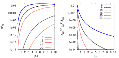
Figure 1: (Left) $R^{p}_{01}$ as a function of $\beta J$ for $c=6$. We can see that as $p$ increases the convergence to the XY model holds up to larger and larger $\beta$ values. For $p=20$ ($p+2=22$), the difference among the two is smaller than double precision up to values of $\beta J\simeq 3$. (Right) Convergence of the $p$-clock paramagnetic free energy to the $XY$ paramagnetic free energy for $c=6$. The denominator is $\bar{f}_{\rm pm}(\beta)\equiv(f_{\rm pm}^{p}+f_{\rm pm}^{XY})/2$. The relative difference between the two decreases with $\beta J$.

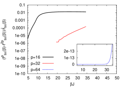
Figure 2: Relative free energy difference of the FM phase for different $p$, $2p$ couples of $p$-clock models. The denominator is $\bar{f}_{\rm fm}(\beta)\equiv(f_{\rm fm}^{(p)}+f_{\rm fm}^{(p+2)})/2$. Already for $p=16$ and $p=32$ the relative difference saturates at $10^{-2}$ for $\beta J>10$. As shown in the inset practically no difference can be appreciated in double precision between $p=64$ and $p=128$ up to $\beta J\simeq 30$.

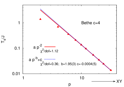
Figure 3: Spinodal temperature, $T_{s}$, as a function of $p$ with its best fits for vanishing $T_{s}$ in the $p\to\infty$ limit for fixed connectivity $c=4$. For continuous $XY$ spins, when $T>0$, the only fixed point solution of $BP$ equations is the paramagnetic solution. The fact that we obtain a ferromagnetic solution is an artifact induced by $p<\infty$.

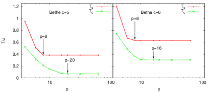
Figure 4: Spinodal and critical temperatures $T_{s}$ and $T_{c}$ vs $p$ in the Bethe lattice, for $c=5$ (left) and $c=6$ (right): the values of $p$ for which convergence to the $XY$ limit is attained are marked by arrows.

In Figs. 3, 4 we report the results obtained for spinodal and critical point as a function of the number of states $p$ for different values of the connectivity $c=4,5,6$. At the critical inverse temperature $\beta_{c}=1/T_{c}$ the PM solution becomes metastable. As we can see from Fig. 3, the lower critical connectivity for the $XY$ model is $c_{\rm low}=5$: FM solutions for $c=4$ are an artifact of taking $\phi$ as a discrete variable. In Fig. 4 we show the convergence to the XY limit in $p$ for $c=5,6$. The convergence is faster for the spinodal point but not much slower for the critical point: $p\simeq 20$-clock spin is already a rather good approximation of the planar continuous spin for what concerns the analysis of the critical behavior.

IV.2 Critical behavior of the 4-XY model

We thus study the properties of the XY model across the critical point using a $p=64$ clock model. In Fig. 5 we display the free energy for $c=6$ as a function of $\beta J$ for the three fixed point solutions of BP equations (27-IV): PM, FM and PL phases. The FM solution is selected by tuning the initial conditions assigning higher probability to a given $\phi$ value. The PL solution is obtained at high enough $\beta$ when initial $\nu(\phi)$ are given with two peaks at opposite angles. In Fig. 6 we report the resulting marginal cavity distributions for the phase values, $\nu(\phi)$ and $\hat{\nu}(\phi)$.

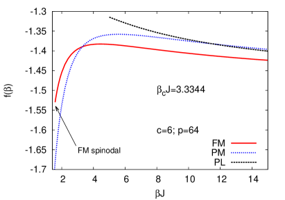
Figure 5: Free energy, $f(\beta)$ vs. $\beta J$ for $c=6$ and $p=64$. The full line refers to the ferromagnetic fixed point solution, found considering as initial conditions the effect of a strong external magnetic field. The dotted line refers to the paramagnetic solution. Unlike in the $k=2$ case, the paramagnetic solution is stable at every temperature. The dashed line represents the metastable phase-locked solution.

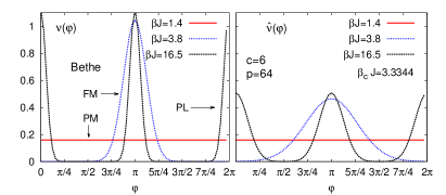
Figure 6: $\nu_{a}$ and $\hat{\nu}_{a}$ for $p=64$ and three different phases at three values of $\beta J$: PM at $\beta J=1.4<\beta_{c}J$, FM at $\beta J=3.8>\beta_{c}J$ and PL at $\beta J=16.5$.

In the PL phase, though at each local instance $m_{xy}=0$, the parameter $r$ defined in Eq. (35) is not. Its free energy behavior is shown in Fig. 5 as dashed line. It can be observed that the PL phase is always metastable with respect to the FM phase, though, for higher $\beta$ its free energy becomes lower than the PM free energy. Because of the observed numerical fragility of such solution with respect to the PM and the FM phases, it is hard to discriminate its spinodal point. With the computation performed so far the PL phase appears to occur for $\beta J\gtrsim 4.5$.

V XY- and $p$-clock models on Erdòs Rényi factor graphs

If the degrees of variable nodes are i.i.d. random variables, the local environment is not the same everywhere in the graph. In the Erdòs Rényi case BP equations are distributional equations as in Eqs. (IV-24) where the number of neighbors to a variable node are extracted by means of a Poissonian distribution of average $c$.

In this section we show the results obtained by applying the PDA on the ordered $p$-clock model on ER graphs and look for asymptotic solutions as $p\rightarrow\infty$. The results presented have been obtained with a population size up to $N=6\cdot 10^{5}$. The code used to numerically determine $\nu,\hat{\nu}$ stationary populations for large $p$ is a parallel code running on GPU’s. This sensitively speeds up the population update of $\hat{\nu}$ (requiring $Np^{k}$ operations) with respect to a serial, CPU running, code.

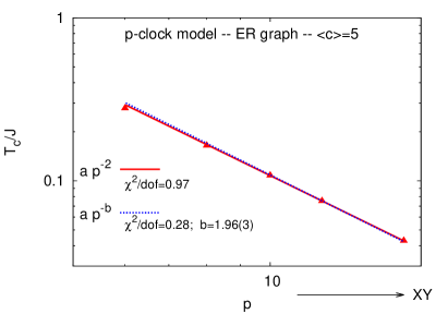
Figure 7: Spinodal point values $T_{s}/J$ vs. $p$ on Erdòs Rényi factor graphs with mean connectivity $\langle c\rangle=5$. The interpolations displayed are both consistence with the absence of a magnetized phase in the XY, for $T>0$.

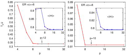
Figure 8: Critical point as a function of integer $p$ on Erdòs Rényi factor graphs with mean connectivity $\langle c\rangle=6$ (left) and $8$ (right). In the insets we show the absolute values of the magnetization as a function of $p$.

In Fig. 7 we show the values obtained for $T_{s}/J$ when the mean connectivity of variable nodes is $\langle c\rangle=5$. We can see that in this case the only solution in the $p\rightarrow\infty$ limit is the PM solution, whereas other solutions with $\langle m^{2}\rangle\neq 0$ are artifacts of $p<\infty$.

In Fig. 8 we report the results obtained when $\langle c\rangle=6$ and $8$: as for regular random graphs the convergence to the $XY$ model is rather fast (see also the inset for the absolute value of the magnetization).

We observe that $c_{\rm low}=6$ for the ER graph is larger than the corresponding value $c_{\rm low}=5$ in the Bethe lattice. The presence of many nodes with connectivity $\langle c\rangle-1$ or lower, when $\langle c\rangle=5$, apparently leads to a zero transition temperature in the ER graph. We notice, however, that in the linear case ($k=2$) the trend is the opposite: for Bethe lattices the minimal connectivity for a non-trivial critical behavior is $c_{\rm low}=3$, for Erdòs Rényi graphs is $c_{\rm low}=2$, as reported in App. A. More details on the linear case can be found in Ref. [Lupo and Ricci-Tersenghi, 2014].

VI Mode-locking on random graphs

As mentioned in the introduction, the nonlinear $XY$ model can be used to describe the phase dynamics of interacting electromagnetic modes in lasers. Previous mean-field studies on fully connected models assume narrow-band for the spectrum, Angelani et al. (2006, 2007); Leuzzi et al. (2009); Conti and Leuzzi (2011) that is, all modes practically have the same frequency and, in this way, the frequencies do not play any role in the system behavior. This is the case for the systems analyzed in Secs. IV and V. In this section, exploiting the diluted nature of the graphs, we deepen such description and allow for the existence of finite-band spectra and gain frequency profiles.

Tree-like factor graphs can be built where each variable node, representing a light mode, has a quenched frequency associated to its dynamic phase. The frequencies are distributed among modes according to, e.g., a Gaussian or a parabolic distribution proportional to the optical gain $g(\omega)$ for the system resonances. The graph is, then, constructed starting from the root in such a way that the FMC Eq. (1) is satisfied for each interacting quadruplet. Else said, a function node $m$ is a FMC for the $\{\partial m\}$ modes connected to it. As an example, in Fig. 9, we show a possible frequency distribution for a tree-like factor graph in which the connectivity of the variable nodes is fixed to $c=6$. The empty (large) triangles refer to the gain profile, $g_{in}(\omega)$, according to which the frequencies are assigned to free variable nodes ($2/3$ of the total). The remaining $1/3$ of the node frequencies are assigned according to the FMC. Note that applying the FMC one can obtain three possible independent combinations for the fourth frequency. From Fig. 9 we can see that the frequency distribution of all frequencies, $g(\omega)$, evaluated once that the FMC has been imposed for the all quadruplets, is compatible with the starting one, $g_{in}(\omega)$. This result shows that, considering a generic Gaussian gain profile, sparse factor graphs, in which $\langle c\rangle=\mathcal{O}(1)$, can yield a meaningful realistic description of non-linearly interacting modes whose frequencies satisfy the FMC.

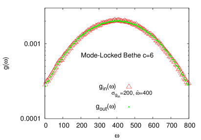
Figure 9: Empty triangles refer to the distribution of frequencies assigned to $2/3$ of the variable nodes, according to a Gaussian gain profile, $g_{in}(\omega)$ of mean $\bar{\omega}=400$ and variance $\sigma_{g_{\rm in}}=200$. Filled-in triangles refer to the distribution $g_{\rm out}(\omega)$ we obtain once the FMC is imposed: $g_{\rm out}(\omega)$ coincides with $g_{in}(\omega)$ on the whole domain.

VI.1 Phases and phase-locking

Once graphs with fixed connectivity and frequency matching function nodes are introduced we can study the critical behavior considering $\beta J$ as a pumping rate squared ${\cal P}^{2}$, cf. Eq. (6), in the context of lasing systems. We will term these graphs “Mode-Locking Bethe” (ML-Bethe) lattices. As a result of BP, above a certain threshold of ${\cal P}$ mode phases turn out to show a peculiar behavior in the frequencies: $\phi(\omega)$ coincides with the linear law of Eq. (2), as shown in Fig. 10 for different linear coefficients $\phi^{\prime}$. Though, generically, the magnetizations are $m_{xy}=0$, the phases are, nevertheless, found to be locked. This is the typical behavior established at the lasing threshold by nonlinearity in multimode lasers. In the above mentioned construction of the ML-Bethe lattice, frequencies are assigned to modes with a probability proportional to the gain profile.

We take into acccount two qualitatively different cases. First we consider the case where only equispaced frequencies are eligible: this is a proxy for the so-called comb distribution Bellini and Hansch (2000); Udem et al. (2002) in which many resonances occurs with a line-width much smaller than the fixed resonance interspacing. Furthermore, we investigate the opposite extreme, the continuous case, in which each mode frequency is extracted continuously from the whole gain band with no further constraint on their values, other than FMC.

Figure 10: Phases vs. frequencies in phase-locked phases on ML-Bethe lattice with $c=6$, $N_{\rm shell}=5$ shells, and a total number of inner nodes (excluding leaves) $N_{\rm bulk}=4339$. The number of clock tics is $p=120$. The number of frequencies is $N_{\omega}=88$ or $120$. The pumping rate squared is ${\cal P}^{2}=\beta J=7$.

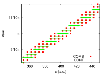
Figure 11: Detail of the behavior of the phases vs. frequencies extracted by means of the distribution of Fig. 9 both as continuous and as comb-like equispaced at $\beta J=7$, for $c=6$, $N_{\rm shell}=4339$, $N_{\rm bulk}=65089$, $p=120$, for $120$ continuous (light grey/green points) and comb (dark grey/red squares) frequencies.

In Fig. 10 we show different realizations of such phase-locking, all of them with different phase delay $\phi^{\prime}$. They are frequency independent and do not depend on frequencies being equispaced or continuously distributed. This amounts to say that phase delay disperion is zero. Each locking is obtained by means of different boundary conditions at the external shell. The case $\phi^{\prime}=0$ is also achieved, that is the ferromagnetic phase: all modes are locked at the same phase. In term of thermodynamics all realizations of phase-locking, including the ferromagnetic one, display comparable free energies, all of them definitely different from the free energy of the coexisting PM phase.

Altough phase-locking, cf. Eq. (2), occurs in both the comb and the continuous frequency distributions, as shown in Fig. 11 there is a difference in the range of values that frequencies can take at each (discrete) value of the phases. We anticipate that only in the case of comb-like distributions of gain resonances mode-locking allows to realize ultrashort pulses.

We, eventually, come to the analysis of the electromagnetic signal for a wave system with $N=N_{\rm bulk}$ modes and $N_{\omega}$ frequencies:

$$E(t) = \sum_{k=1}^{N}A_{k}e^{\imath(\omega_{k}t+\phi_{k})}$$ (37)

$$= e^{\imath(\omega_{0}t+\phi_{0})}\sum_{k=1}^{N}A_{k}e^{\imath(\Delta\omega_{k}t+\Delta\phi_{k})}$$

where the sinusoidal carrier wave frequency $\omega_{0}$ is the central frequency of the spectrum (of the order of $10^{15}$ rad $\cdot$ s^-1), $\phi_{0}=\phi(\omega_{0})$ and $\Delta\omega_{k}$’s are of the order of radio frequencies (ca. $10^{9}$ rad $\cdot$ s^-1). In the ML regime, where, cf. Eq. (2), $\Delta\phi_{k}=\phi^{\prime}\Delta\omega_{k}$ the time dependent overall amplitude can be written as

$$A(t) \equiv \sum_{k=1}^{N}A_{k}e^{\imath(\Delta\omega_{k}t+\Delta\phi_{k})}$$

$$= \sum_{k=1}^{N}A_{k}e^{\imath\Delta\omega_{k}(t+\phi^{\prime})}=A(t+\phi^{\prime})$$

The term phase (or group) delay for $\phi^{\prime}$ comes from the fact that it corresponds to a shift in time in the $E(t)$ carrier peak with respect to the $|E(t+\phi^{\prime})|=|A(t+\phi^{\prime})|$ envelope maximum. If, furthermore, $N_{\omega}$ comb distributed resonances are considered with interspacing $\Delta\omega$, we can write

$$e^{\imath\Delta\omega_{k}t}=n_{l}e^{\imath l\Delta\omega t};$$ (39)

$$\quad k=1,\ldots,N;\quad l=-N_{\omega}/2,\ldots,N_{\omega}/2-1$$

where $n_{l}$ is the number of modes at frequency $l\Delta\omega$. This is the case for ultra-short ML lasers for which very short and very intense periodic pulses occur, as shown for $N_{\rm bulk}=4339$ modes in the first and third left panels in Fig. 12 for $\phi^{\prime}=0.0314$ ($N_{\omega}=120$) and $\phi^{\prime}=0.0075$ ($N_{\omega}=88$), respectively.

Since we are working in the quenched amplitude approximation with intensity equipartition each mode has magnitude $A_{k}=1$. However, we are using diluted interaction networks and, consequently, the same frequency can be taken by modes localized in different spatial regions, whose number we denote by $n_{l}$ in Eq. (39). Therefore,

$$E(t)=e^{\imath(\omega_{0}t+\phi_{0})}\sum_{l=-N_{\omega}/2}^{N_{\omega}/2-1}n_{l}~{}e^{\imath l\Delta\omega(\phi^{\prime}+t)}$$ (40)

and, from the point of view of the Fourier decomposition of the e.m. signal, $n_{l}$ plays the role of the amplitude of the modes at frequency $l$.

A detail of the pulses is shown in the first and third right panels of Fig. 12. The linear behaviors shown in Fig. 10, alike to Eq. (2), implies that the signal is unchirped. Else said, the phase delay displays no dispersion and the frequency of oscillation of the carrier remains the same for all pulses, as can be observed in the right panels of Fig. 12. The period of the pulses is $\tau_{p}=2\pi/\Delta\omega$, where $\Delta\omega=5$ for phase delay $\phi^{\prime}=0.0314$ and $\Delta\omega=7$ for $\phi^{\prime}=0.0075$. The pulse duration is expressed in terms of its Full Width Half Maximum $\Delta\tau_{p}$, also equal to the time it takes for the e.m. field amplitude $A(t)$, to decrease to zero from its maximum.

In ML ultrafast lasers, if the gain has a Gaussian profile in the equidistant frequencies, and ,consequently, $n_{l}$ is so distributed, cf. Eq. (40), the signal amplitude squared is expected to behave like

$$|E(t)|^{2}=|E(t_{\rm max})|^{2}\exp\left\{-\left(2\frac{t-t_{\rm max}}{\Delta\tau_{p}}\right)^{2}\ln 2\right\}$$ (41)

in the limit of very many frequencies ($\Delta\omega\to 0$).Svelto (1998) In Fig. 12, first and third right panels, this behavior is plotted as “Gaussian”. Above the noise level it appears to coincide very well with the envelope obtained by Fourier Transform of the output of BP equations on ML Bethe lattices.

In the second ($\phi^{\prime}=0.0314$) and fourth ($\phi^{\prime}=0.0075$) rows of Fig. 12 we show $E(t)$ in the low pumping paramagnetic phases, where modes display random phases (RP). The periodicity induced by the comb-like distribution appears also here, though the electromagnetic field is purely noisy, without any pulse.

When frequencies are taken in a continuous way the coherent phase-locked phase turns out to display much less intense coherent signal, with no pulses, as shown in Fig. 13 where $|E(t)|$ is shown both in the ML and in the random phase (paramagnetic) regimes, with no apparent difference in the time domain between coherent and incoherent light.

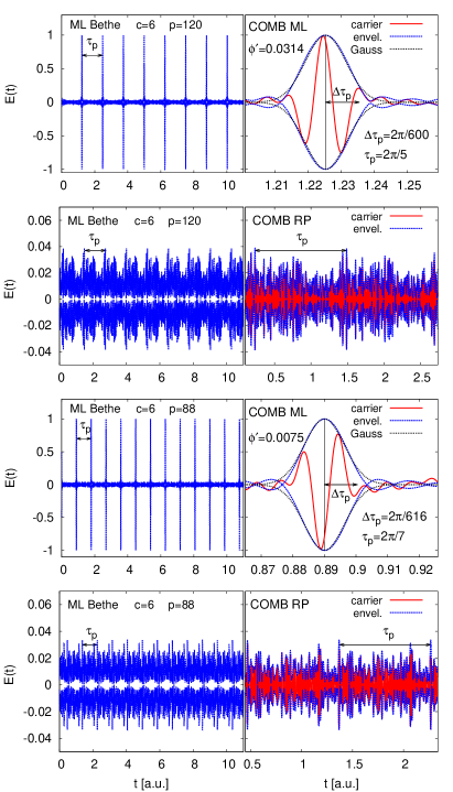
Figure 12: The laser pulse $E(t)$ generated in the lasing phase in a ML Bethe lattice with comb-like frequency distribution. Two different realizations of the phase-locking are reported, with delay $\phi^{\prime}=0.0314$ (top four panels) and $\phi^{\prime}=0.0075$ (bottom four panels). In the left panels several periodc pulses are shown, with a period $\tau_{p}=2\pi/\Delta\omega$, with $\Delta\omega=5$ in the top case and $\Delta\omega=7$ in the bottom case. In the right panels the details of the single pulse are given, where both carrier and envelope are plotted. In the ML pulsed phase (first and third right panels) the pulse half-width is $\Delta\tau_{p}=2\pi/(N\Delta\omega)$, where $N=120$ for $\phi^{\prime}=0.0314$ and $N=88$ for $\phi^{\prime}=0.0075$. We also plot the behavior of the amplitude $\pm|E(t)|$ expected for Gaussian gain profiles, i.e., the square root of (41), displaying a rather good coincidence.

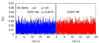
Figure 13: The amplitude of the e.m. field, $|E(t)|$, cf. Eq. (VI.1), is plotted for a ML Bethe lattice with continuously frequency distribution. In the first row we display the $\phi^{\prime}=0.0314$ case in the high pumping mode-locked regime (left) and in the low pumping random phase regime (right). In the second row $\phi^{\prime}=0.0075$.

VII Conclusions

In the present work we have undergone the investigation of the $XY$ model with non-linear, $4$-body, interaction and of its discrete approximant, the so-called $p$-clock model, on random graphs. Cavity equations have been derived and solved for the Bethe lattice and the Erdós-Rényi graph, carrying out a thourough analysis of the critical behavior in temperature at varying connectivity values. Three phases are found for these models. At high $T$ the systems are in a paramagnetic phase. At low $T$ the dominat thermodynamic phase is ferromagnetic, that is, a $SU(2)$ continuous symmetry breaking occurs in the XY model and a $Z_{p}$ discrete symmetry breaking occurs in the $p$-clock model. Else, a low temperature metastable phase-locking phase can be reached, in which the magnetization is zero but the phases, though all different, are nevertheless correlated to each other. An accurate study of the convergence of the $p$-clock model to the continous model is performed and presented.

The models introduced can be applied to laser optics, where the $XY$ or $p$-clock spins play the role of light mode phases. In this photonic framework the inverse temperature $\beta$ is proportional to the square of the rate of population inversion, the so-called pumping rate, driving the lasing transition from the incoherent light regime. The first result is that a mode-locking Bethe lattice can be consistently built in which, besides the phase, also a frequency is associated to each variable node and each function node acts as a frequency matching condition among four frequencies, cf. Eq. 1. The latter is a common kind of non-linear interaction occurring in standard ultra-fast multimode lasers. As $\beta$ increases the system is found to undergo a mode-locking transition: phases at nearby frequencies are locked to take fixed amount and a linear $\phi(\omega)$ relationship like Eq. (2) is established at the critical point. In the case of evenly distributed mode frequencies this leads to a pulsed laser, i.e., a laser whose electromagnetic field oscillations are characterized by a train of very short and very intense pulses. We have been comparing the results obtained in this case to the laser signal for multimode frequencies randomly taken in a continuous dominion, as well as to the incoherent signal below the lasing threshold. The model presented, thus, provides an analytical and phenomenologically accurate description of multimode lasers at the level of the single pulse, that can be chosen arbitrarily shorter than the period between two pulses when the frequencies are evenly spaced as, e.g., in standard Fabry-Perot cavities. Such a limit is not achievable experimentally because the typical response time of conventional photodetectors is of the order of $1$ ns, whereas the duration of pulses in ultra-fast mode-locking solid-state or semiconductor lasers ranges from the order of the picosecond to the order of the femtosecond.

Eventually, laser emission is also investigated in the opposite extreme, where frequencies can take any value according to a given gain profile, not only evenly spaced values. These systems undergo phase-locking, because of the frequency matching condition, but prove a far less intense signal, more akin to the signal of early continuous-wave pumped solid-state lasers. Nelson and Boyle (1962) Such frequency limit distribution is, in principle, compatible with the random topology of light localizations on sparsely connected interaction networks that can represent a salient feature of more complex laser systems called random lasers.Lawandy et al. (1994); Cao et al. (1999); Cao (2005); Wiersma (2008) In these systems, indeed, where also the magnitude and even the sign of the mode coupling can be disordered, the pumping rate threshold values are known to be higher and the signal intensity is found to be sensitively smaller than in standard ordered multimode lasers.

Appendix A XY model with linear interaction on sparse graphs

Let us consider the two point correlation function for the $XY$ model with pairwise interaction, $k=2$:

$$\mathcal{H}=-\sum_{(i,j)}J_{ij}\cos{\left(\phi_{i}-\phi_{j}\right)}$$ (42)

Taking two variable nodes, $i$ and $j$, we indicate by $U_{ij}$ the shortest path that goes from $i$ to $j$, by $F_{R}$ the subset of function nodes (now simple links) in $U_{ij}$ and by $V_{R}$ the subset of variable nodes in $U_{ij}$ including $i$ and $j$. Then let $\partial R$ be the subset of function nodes that are not in $U_{ij}$ but are adjacent to the variable nodes in $V_{R}$: $\forall m\in\partial R$, $\exists^{\prime}$ $l\in\partial m\bigcap V_{R}$, which will be called $l(m)$. Then, we have that the joint probability distribution of all variables in $R$ is:

$$\mu\left(\underline{\phi_{R}}\right)=\frac{1}{Z_{R}}\prod_{m\in F_{R}}\psi_{m}\left(\phi_{\partial m}\right)\prod_{m\in\partial R}\hat{\nu}_{m\rightarrow l(m)}\left(\phi_{l(m)}\right)$$ (43)

We, then, denote by $r$ the distance between the two initial spins $i$ and $j$. The distance $r$ is, in fact, the number of links in $F_{R}$, each one with its marginal $\hat{\nu}$. Recalling Eq. 11 we obtain that, in the paramagnetic phase (where $\hat{\nu}(\phi)=\frac{1}{2\pi}$, $\forall\phi\in[0,2\pi)$), the two-spin joint probability distribution function is:

$$\mu(\phi_{i},\phi_{j}) = \frac{1}{(2\pi)^{2}}+\frac{1}{(\pi~{}I_{0}(\beta J))^{r}}$$

$$\quad\times\sum_{n=1}^{\infty}\left(I_{n}(\beta J)\right)^{r}\cos(n(\phi_{i}-\phi_{j}))$$

Consequently, it is

$$\langle\cos(\phi_{i})\cos(\phi_{j})\rangle=\langle\sin(\phi_{i})\sin(\phi_{j})\rangle=\frac{1}{2}\left(\frac{I_{1}(\beta J)}{I_{0}{\beta J}}\right)^{r}$$

and

$$C(r)\equiv\langle\cos(\phi_{i}-\phi_{i+r})\rangle=\left(\frac{I_{1}(\beta J)}{I_{0}(\beta J)}\right)^{r}$$ (45)

The susceptibility can be written as

$$\chi=\frac{1}{N}\sum_{r=0}^{\infty}\sum_{(i,j=i+r)\in\mathcal{G}}\langle\sigma_{i}\sigma_{j}\rangle=\sum_{r=0}^{\infty}\mathcal{N}(r)\left(\frac{I_{1}(\beta J)}{I_{0}(\beta J)}\right)^{r}$$ (46)

where $(i,i+r)$ indicates all the links in the graph between two variable nodes at distance $r$ and $\mathcal{N}(r)$ is the expected number of variables nodes $j$ at a distance $r$ from a uniformly random node $i$. For large $r$ on a Bethe graph $\mathcal{N}(r)=(c-1)^{r}$ and $\chi<\infty$ for

$$\left(\frac{I_{1}(\beta J)}{I_{0}(\beta J)}\right)(c-1)<1$$ (47)

As

$$\left(\frac{I_{1}(\beta_{c}J)}{I_{0}(\beta_{c}J)}\right)(c-1)=1$$ (48)

$\chi=\infty$, the paramagnetic solution becomes unstable and the value of the critical temperature $T_{c}=\frac{1}{\beta_{c}}$ is determined.

For the case of Erdòs Rényi graphs, we obtain for large $r$ $\mathcal{N}(r)=\langle c\rangle=c$ where we used the property of the Poissonian distribution $P_{c}(k)$, with $k=c-1$:

$$\sum_{c=2}^{\infty}(c-1)P_{c}(c-1) = \sum_{c=2}^{\infty}e^{-c}\frac{c^{c-1}}{(c-1)!}(c-1)$$

$$= c~{}e^{-c}\sum_{c=2}^{\infty}\frac{c^{c-2}}{(c-2)!}=c$$

Then, in this case Eq. 48 becomes:

$$\left(\frac{I_{1}(\beta_{c}J)}{I_{0}(\beta_{c}J)}\right)(c)=1$$ (50)

We stress that both critical conditions Eqs. 48 and 50 can be obtained by expanding Eq. 11 around the paramagnetic solution Skantzos et al. (2005); Lupo and Ricci-Tersenghi (2014). In the ER case we see that the presence of nodes with connectivity larger than $c$ has the effect of lowering $\beta_{c}$, i.e. increasing $T_{c}$.

References

- Kosterlitz and Thouless (1972) J. Kosterlitz and D. Thouless, J.Phys.C 5, L124 (1972).
- Brézin (1982) E. Brézin, J. de Phys. (France) 43, 15 (1982).
- Brézin (2010) E. Brézin, Introduction to Statistical Field Theory (Cambridge University Press, 2010).
- Cardy (1996) J. Cardy, Scaling and Renormalization in Statistical Physics (Cambridge University Press, Cambridge, 1996).
- Kuramoto (1975) Y. Kuramoto, Lect. N. Phys. 39, 420 (1975).
- Acebrón et al. (2005) J. A. Acebrón, L. L. Bonilla, C. J. Pérez Vicente, F. Ritort, and R. Spigler, Rev. Mod. Phys. 77, 137 (2005).
- Gupta et al. (2014) S. Gupta, A. Campa, and S. Ruffo, J. Stat. Mech. p. R08001 (2014).
- Angelani et al. (2007) L. Angelani, C. Conti, L. Prignano, G. Ruocco, and F. Zamponi, Phys. Rev. B 76, 064202 (2007).
- Gordon and Fischer (2002) A. Gordon and B. Fischer, Phys. Rev. Lett. 89, 103901 (2002).
- Angelani and Ruocco (2007) L. Angelani and G. Ruocco, Phys. Rev. E 76, 051119 (2007).
- Antenucci et al. (2014a) F. Antenucci, C. Conti, A. Crisanti, and L. Leuzzi, arXiv:1409.7826 (2014a).
- Angelani et al. (2006) L. Angelani, C. Conti, G. Ruocco, and F. Zamponi, Phys. Rev. Lett. 96, 065702 (2006).
- Leuzzi et al. (2009) L. Leuzzi, C. Conti, V. Folli, L. Angelani, and G. Ruocco, Phys. Rev. Lett. 102, 083901 (2009).
- Conti and Leuzzi (2011) C. Conti and L. Leuzzi, Phys. Rev. B 83, 134204 (2011).
- Antenucci et al. (2014b) F. Antenucci, M. "Ibáñez Berganza", and L. Leuzzi, arXiv:1409.6345 (2014b).
- Murray Sargent III, Marlan O’Scully and Willis E. Lamb (1978) Murray Sargent III, Marlan O’Scully and Willis E. Lamb, Laser Physics (Addison Wesley Publishing Company, 1978).
- Haus (1984) H. A. Haus, Waves and Fields in Optoelectronics (Prentice-Hall, Englewood Cliffs, N. J., 1984).
- Haus (2000) H. A. Haus, IEEE J. Quantum Electron. 6, 1173 (2000).
- Gordon and Fischer (2003) A. Gordon and B. Fischer, Opt. Comm. 223, 151 (2003).
- Mézard and Montanari (2009) M. Mézard and A. Montanari, Information, Physics, and Computation (Oxford University Press, 2009).
- Mézard et al. (1987) M. Mézard, G. Parisi, and M. A. Virasoro, Spin glass theory and beyond (World Scientific, Singapore, 1987).
- Mézard and Parisi (2001) M. Mézard and G. Parisi, Eur. J. Phys. B 20, 217 (2001).
- Lupo and Ricci-Tersenghi (2014) C. Lupo and F. Ricci-Tersenghi, in preparation (2014).
- Bellini and Hansch (2000) M. Bellini and T. W. Hansch, Opt.Lett. 25, 1049 (2000).
- Udem et al. (2002) T. Udem, R. Holzwarth, and T. Hansch, Nature 416, 233 (2002).
- Svelto (1998) O. Svelto, Principles of lasers (Springer, 1998).
- Nelson and Boyle (1962) D. F. Nelson and W. S. Boyle, Appl. Opt. 1, 181 (1962).
- Lawandy et al. (1994) N. M. Lawandy, R. M. Balachandran, A. S. L. Gomes, and E. Sauvain, Nature 368, 436 (1994).
- Cao et al. (1999) H. Cao, Y. G. Zhao, S. T. Ho, E. W. Seelig, Q. H. Wang, and R. P. H. Chang, Phys. Rev. Lett. 82, 2278 (1999).
- Cao (2005) H. Cao, J. Phys. A. : Math. Gen. 38, 10497 (2005).
- Wiersma (2008) D. S. Wiersma, Nature Physics 4, 359 (2008).
- Skantzos et al. (2005) N. S. Skantzos, I. P. Castillo, and J. P. L. Hatchett, Phys. Rev. E 72 (2005).