Joint Association Graph Screening and Decomposition for Large-scale Linear Dynamical Systems

Abstract

This paper studies large-scale dynamical networks where the current state of the system is a linear transformation of the previous state, contaminated by a multivariate Gaussian noise. Examples include stock markets, human brains and gene regulatory networks. We introduce a transition matrix to describe the evolution, which can be translated to a directed Granger transition graph, and use the concentration matrix of the Gaussian noise to capture the second-order relations between nodes, which can be translated to an undirected conditional dependence graph. We propose regularizing the two graphs jointly in topology identification and dynamics estimation. Based on the notion of joint association graph (JAG), we develop a joint graphical screening and estimation (JGSE) framework for efficient network learning in big data. In particular, our method can pre-determine and remove unnecessary edges based on the joint graphical structure, referred to as JAG screening, and can decompose a large network into smaller subnetworks in a robust manner, referred to as JAG decomposition. JAG screening and decomposition can reduce the problem size and search space for fine estimation at a later stage. Experiments on both synthetic data and real-world applications show the effectiveness of the proposed framework in large-scale network topology identification and dynamics estimation.

I Introduction

Topology learning and parameter estimation of dynamical networks have become popular research topics recently because such studies can reveal the underling mechanisms of many real-world complex systems. For example, a stock market which consists of a large number of stocks interacting with each other and evolving over time can be characterized as a dynamical network. Here, a node stands for the price of a stock and an edge or link resembles stock interaction. Let $\boldsymbol{x}$ be a $p$-dimensional random vector with each component being a time series associated with a node. We are interested in inferring the topology and dynamics of a linear dynamical network $\boldsymbol{x}_{t}=\boldsymbol{A}\boldsymbol{x}_{t-1}+\boldsymbol{\epsilon}_{t}$, with $\boldsymbol{\epsilon}_{t}$ as the system disturbance. Such a model has been proposed and studied in many areas such as econometrics, finance and bioinformatics [1, 2, 3, 4]. The transition matrix $\boldsymbol{A}$ determines how the current state of the network evolves from the previous state. It can be translated to a directed Granger transition graph (GTG) that shows the Granger causal connections between the nodes [5, 6, 7]. The modern challenge is that the number of unknowns in $\boldsymbol{A}\in\mathbb{R}^{p\times p}$ is usually much larger than the number of available observations $\boldsymbol{x}_{1},\cdots,\boldsymbol{x}_{n}$, i.e., $p^{2}\gg n$, and consequently most conventional methods fail in estimation or identification. From a statistical perspective, shrinkage estimation [8] must be applied, and sparsity-promoting regularizations are preferred because they can produce interpretable networks [9, 10]. Indeed, in many applications, there only exist a few significant nodes that directly influence a given node. Sparse graph learning also complies with the principle of Occam’s razor from a philosophical perspective. Nevertheless, existing methods usually assume that the components of $\boldsymbol{\epsilon}_{t}$ are i.i.d., i.e., the covariance matrix of $\boldsymbol{\epsilon}_{t}$, or $Cov(\boldsymbol{x}_{t}|\boldsymbol{x}_{t-1})$, is proportional to the identity matrix. This totally ignores the second-order statistical structure of the network. Most real-world networks violate this assumption because even conditioning on past observations, node correlations widely exist.

Assuming, ideally, the true $\boldsymbol{A}$ is known, the dependence structure of a network can be captured by the sparse Gaussian graph learning, which has attracted a lot of research attention lately (cf. [11, 12, 13, 14] among many others). Under $\boldsymbol{\epsilon}_{t}\sim N(\boldsymbol{0},\boldsymbol{\Sigma})$, the $(i,j)$th entry of the concentration matrix $\boldsymbol{\Omega}\triangleq\boldsymbol{\Sigma}^{-1}$ gives the conditional dependence between node $i$ and node $j$ given all the other nodes. This can be translated to an undirected conditional dependence graph (CDG), in which case, again, sparsity on $\boldsymbol{\Omega}$ is desirable. Unfortunately, Gaussian graph learning is not directly applicable to our dynamical model, because as discussed above, the task of estimating $\boldsymbol{A}$ is no less challenging as the task of estimating $\boldsymbol{\Omega}$. Note that substituting the sample mean for the true mean is inappropriate when $\boldsymbol{A}$ is a large matrix, which is a well known example of Stein’s phenomenon [8].

To obtain a comprehensive picture of the dynamical network, it is necessary to estimate both $\boldsymbol{A}$ and $\boldsymbol{\Omega}$ based on their joint likelihood. There are few studies in the literature that consider the joint sparse estimation of the two matrices [15, 16]. In our experience, the existing methods are slow and can not handle big network data. For example, the MRCE algorithm [15] is already infeasible for $p>120$ on an ordinary PC. Note that the number of unknown variables, $p^{2}+p(p+1)/2$, can be very large, thereby making it difficult to reliably identify the sparse network topology and accurately estimate the system parameters.

As a real example, we use the Energy category of the S&P 500 stock data to illustrate our motivation. Figure 1 shows the graphs obtained by sole GTG learning (sGTG for short) which ignores the second-order node correlations, and by sole CDG learning (sCDG for short) which ignores the first-order Granger causalities. Common isolated nodes have been removed. Some edges exist in both graphs, which suggests that the joint regularization of $(\boldsymbol{A}$, $\boldsymbol{\Omega})$ might be helpful in detecting the joint graphical structure. In fact, statistically speaking, even when similarities between the two graphs are not clear or even do not exist, joint regularization can improve the overall estimation accuracy in high dimensions, see, e.g., [8, 17]. Another interesting observation from Figure 1 is that the network can be decomposed into smaller subnetworks including isolated indices. Similar decomposability has also been noticed in brain connectivity networks [18] and U.S. macroeconomics [19]. If such a network decomposition could be detected in an early stage, complex learning algorithms, such as MRCE and Gaussian graph learning, would apply in a much more efficient way (in a possibly parallel manner). Of course, the decomposition based on sGTG or sCDG alone may not be trustworthy. When $p$ is large and both GTG and CDG are unknown, the graph screening/decomposition based on $\boldsymbol{A}$ and $\boldsymbol{\Omega}$, jointly, is much more reasonable.

(a) sGTG

(b) sCDG

Figure 1: The sGTG and sCDG for the $S\&P$ 500 indices from the “Energy” category. Common isolated nodes have been removed. Two nodes are connected with a line (directed in GTG, undirected in CDG) if and only if their connection weight is nonzero.

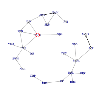
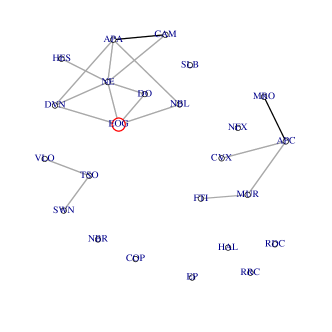
This work proposes jointly regularizing the directed transition graph and the undirected dependence graph for topology identification and dynamics estimation. We will introduce the notion of joint association graph (JAG) and propose JAG screening and decomposition to facilitate large-scale network learning. The JAG screening identifies and removes unnecessary links. The JAG structure can also be used for network decomposition, so that GTG or CDG can be estimated for each subnetwork separately. With search space and problem size substantially reduced, computational and statistical performance can be enhanced. Similar ideas have proved to be very successful in Gaussian graph learning, such as the block diagonal screening rule (BDSR) [20, 21]. Our approach is based on JAG instead of CDG alone. Moreover, we will develop a robust JAG decomposition that does not incur excessive estimation bias as BDSR does [22]. Our approach does not mask authentic edges to guarantee decomposability. To the best of our knowledge, no work of joint graph screening or decomposition is available in the literature.

The remainder of this paper is organized as follows. Section II describes the joint graphical model and proposes a learning framework called joint graphical screening and estimation (JGSE). Section III develops an algorithm of graphical iterative screening via thresholding to be used for JAG screening and robust decomposition. Section IV gives a fine learning of graphs (FLOG) algorithm that estimates $\boldsymbol{A}$ and $\boldsymbol{\Omega}$ after screening. In Section V, synthetic-data experiments are conducted to show the performance of JGSE. In Section VI, we apply JGSE to real S&P 500 and NASDAQ-100 stock data for network learning.

II The joint graphical model

Suppose there exist $p$ nodes in a dynamical network and let $\boldsymbol{x}$ be a $p$-dimensional random vector with each component associated with a node. To describe the node behaviors at each time point, we define a linear dynamical network model

$$\boldsymbol{x}_{t}=\boldsymbol{A}\boldsymbol{x}_{t-1}+\boldsymbol{\epsilon}_{t},\quad\boldsymbol{\epsilon}_{t}\sim\mathcal{N}(\boldsymbol{0},\boldsymbol{\Sigma}).$$ (1)

The current state of the system is determined by two components: The first component is a linear transformation of the previous state; the second component $\boldsymbol{\epsilon}_{t}$ follows a multivariate Gaussian distribution and characterizes node correlations conditioned on $\boldsymbol{x}_{t-1}$. The transition matrix $\boldsymbol{A}$ can be translated to a directed Granger transition graph (GTG): $a_{ij}\neq 0$ indicates that node $j$ Granger-causes node $i$ [5]. The concentration matrix $\boldsymbol{\Omega}\triangleq\boldsymbol{\Sigma}^{-1}$ can be translated to an undirected conditional dependence graph (CDG): $\omega_{ij}=\omega_{ji}=0$ indicates that node $i$ and node $j$ are conditionally independent given the other nodes [11, 12] and $\boldsymbol{x}_{t-1}$. Given $n+1$ snapshots of the system, $\boldsymbol{x}_{1},\cdots,\boldsymbol{x}_{n+1}$, we would like to recover the first-order statistic $\boldsymbol{A}$ and the second-order statistic $\boldsymbol{\Omega}$ as well as find out their sparsity patterns (or topological structures). We are particularly interested in dynamical networks with both GTG and CDG being sparse or approximately sparse for the following reasons. First, many real-world dynamical networks are indeed sparse. For example, in regulatory networks, a gene is only regulated by several other genes [3]. Second, when the number of observations is small compared with the number of unknown variables, the sparsity assumption reduces the number of model parameters so that estimating the system becomes possible. Third, from a philosophical point of view, a sparse model is consistent with the principle of Occam’s razor and is easier to interpret in practice.

As pointed out by a referee, sCDG which estimates $Cov(\boldsymbol{x}_{t})$ typically yields a less sparse graph than $\boldsymbol{\Sigma}^{-1}$, because the transition matrix $\boldsymbol{A}$, together with the autoregressive mechanism, brings in further node dependence (see, e.g., [23] for more details).

II-A Joint regularization in network learning

Using the Markov property and chain rule, we can write the joint likelihood of $\boldsymbol{A}$ and $\boldsymbol{\Omega}$ (conditioned on $\boldsymbol{x}_{1}$) as $l(\boldsymbol{A},\boldsymbol{\Omega})=f(\boldsymbol{x}_{n+1},\cdots,\boldsymbol{x}_{2}|\boldsymbol{x}_{1},\boldsymbol{A},\boldsymbol{\Omega})=\prod_{t=1}^{n}f(\boldsymbol{x}_{t+1}|\boldsymbol{x}_{t},\boldsymbol{A},\boldsymbol{\Omega})$. So the joint ML estimation solves $\min_{\boldsymbol{A},\boldsymbol{\Omega}\succ 0}\frac{1}{2}\sum_{t=1}^{n}(\boldsymbol{x}_{t+1}-\boldsymbol{A}\boldsymbol{x}_{t})^{\mathsf{T}}\boldsymbol{\Omega}(\boldsymbol{x}_{t+1}-\boldsymbol{A}\boldsymbol{x}_{t})-\frac{n}{2}\log|\boldsymbol{\Omega}|.$ Let $\boldsymbol{Y}=[\boldsymbol{x}_{2},\cdots,\boldsymbol{x}_{n+1}]^{\mathsf{T}},\boldsymbol{X}=[\boldsymbol{x}_{1},\cdots,\boldsymbol{x}_{n}]^{\mathsf{T}}$ and $\boldsymbol{B}=\boldsymbol{A}^{\mathsf{T}}$. We write the ML problem in matrix form

$$\min_{\begin{subarray}{c}\boldsymbol{B},\boldsymbol{\Omega}\in\mathbb{R}^{p\times p}\\ \boldsymbol{\Omega}\succ 0\end{subarray}}L(\boldsymbol{B},\boldsymbol{\Omega})=\frac{1}{2}\mbox{tr}\{(\boldsymbol{Y}-\boldsymbol{X}\boldsymbol{B})\boldsymbol{\Omega}(\boldsymbol{Y}-\boldsymbol{X}\boldsymbol{B})^{{\mathsf{T}}}\}-\frac{n}{2}\log|\boldsymbol{\Omega}|.$$ (2)

Here $\boldsymbol{\Omega}\succ 0$ means that $\boldsymbol{\Omega}$ is positive definite (which implies that $\boldsymbol{\Omega}$ is symmetric). From now on, we use $\boldsymbol{B}$, in place of $\boldsymbol{A}$, to represent the GTG.

To enforce sparsity, a straightforward idea is to add penalties, $P_{B}(\boldsymbol{B};\lambda_{B})$ and $P_{\Omega}(\boldsymbol{\Omega};\lambda_{\Omega})$, to the loss in (2). $P_{B}$ and $P_{\Omega}$ can be of the $\ell_{1}$ type [24, 25, 15]. In this paper, we propose jointly regularizing $\boldsymbol{B}$ and $\boldsymbol{\Omega}$ via penalty $P_{C}(\boldsymbol{C}(\boldsymbol{B},\boldsymbol{\Omega});\lambda_{C})$, where $\boldsymbol{C}$ is constructed based on $\boldsymbol{B}$ and $\boldsymbol{\Omega}$. This leads to the following optimization problem

$$\min_{\boldsymbol{B},\boldsymbol{\Omega}\succ 0}L(\boldsymbol{B},\boldsymbol{\Omega})+P_{C}(\boldsymbol{C}(\boldsymbol{B},\boldsymbol{\Omega});\lambda_{C})+P_{B}(\boldsymbol{B};\lambda_{B})+P_{\Omega}(\boldsymbol{\Omega};\lambda_{\Omega}).$$ (3)

The design of $P_{C}(\boldsymbol{C}(\boldsymbol{B},\boldsymbol{\Omega});\lambda_{C})$ is to capture the joint structure of GTG and CDG. Of course, joint regularization can reinforce the detection of common edges if they exist. But why does one care about the joint graphical structure in computation and statistics? Some motivations are given below.

1) First, due to the sparsity assumption on $\boldsymbol{A}$ and $\boldsymbol{\Omega}$, the union of the two graphs is still sparse. That is, many nodes have no direct influences. Hence one can perform graph screening in an earlier stage for dimension reduction, to facilitate fine GTG and CDG learnings afterwards. A good screening process should take both graphs into account in removing unnecessary hypothetical edges.

2) Many very large dynamical networks demonstrate smaller-scale subnetwork structures or clusters. For example, a human brain connectivity network revealed by EEG data can be divided into several functionality regions [18]. Also, in the U.S. macroeconomic network, economic indices can be divided to different categories [19]. It is desirable to decompose a large-scale network into small subnetworks, if possible, for both computational and statistical concerns  [20, 21]. In the dynamical network setting, such a decomposition must be based on both GTG and CDG.

3) Finally, the joint regularization helps improve the overall identification and estimation accuracy based on some classical statistics literature [8, 17, 26].

II-B Joint association graph

Model (1) shows the network evolves through both first-order and second-order statistical relations between the nodes. To capture the joint structure, we introduce the notion of joint association graph (JAG), an undirected graph where any two nodes are connected if they are connected in either GTG or CDG. Define the “association strength” between node $i$ and node $j$ as

$$c_{ij}=c_{ji}=\sqrt{b_{ij}^{2}+b_{ji}^{2}+2\phi^{2}\omega_{ij}^{2}},$$ (4)

where $\phi$ is a weight parameter (say, $\phi=1$); the matrix $\boldsymbol{C}=[c_{ij}]\in\mathbb{R}^{p\times p}$ represents the JAG.

To give an illustration of JAG, we show a toy example in Figure 2, where the JAG in Figure 2c is obtained from (4). The GTG and CDG share many common edges. Furthermore, they both exhibit subnetwork structures. In fact, in both graphs, nodes 1-4 form a cluster. On the other hand, the two graphs differ from each other in some significant ways. For example, node 9 and node 10 are disconnected in GTG, but not so in CDG. JAG, by integrating the connections in GTG and CDG, provides a comprehensive picture of the network topology.

(a) GTG

(b) CDG

(c) JAG

Figure 2: Demonstration of the joint graphical model.

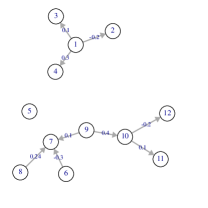
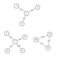
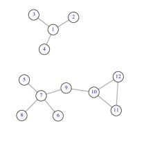
In reality, both the GTG and CDG are unknown and to be estimated. If one had the JAG learned beforehand, its structure could be used to perform graph screening and help improve the estimation of $\boldsymbol{B}$ and $\boldsymbol{\Omega}$. For example, in Figure 2c, node 4 and node 5 are disconnected, so setting $b_{45}=b_{54}=\omega_{45}=\omega_{54}=0$ beforehand facilitates network estimation and identification. Particularly, if the JAG, after permutation, exhibits a block-diagonal structure—$\mbox{diag}\{\boldsymbol{C}_{11},\cdots,\boldsymbol{C}_{dd}\}$, then both $\boldsymbol{B}$ and $\boldsymbol{\Omega}$ must have the same block-diagonal structure, $\mbox{diag}\{\boldsymbol{B}_{11},\cdots,\boldsymbol{B}_{dd}\}$ and $\mbox{diag}\{\boldsymbol{\Omega}_{11},\cdots,\boldsymbol{\Omega}_{dd}\}$, respectively. It is not difficult to show that such a network can be decomposed into $d$ independent subnetworks with its dynamics properties completely intact. For example, the network shown in Figure 2 can be decomposed into two mutually disconnected subnetworks according to its JAG. We can estimate and infer GTG and CDG for each subnetwork separately. Explicitly estimating the JAG based on (4) also facilitates computation and algorithm design, as will be shown in Section III-B.

II-C The JGSE learning

Directly tackling the jointly regularized problem (3) is extremely challenging. (Even without $P_{C}$, the existing algorithms are inefficient or even infeasible for moderate-scale problems.) The key of the paper is to detect and utilize the joint structure of $\boldsymbol{B}$ and $\boldsymbol{\Omega}$ for computational and statistical performance boost. We propose a Joint Graphical Screening and Estimation (JGSE) learning framework which consists of two stages: 1) JAG screening and decomposition; 2) fine estimation.

In Stage 1, we identify the structure of JAG by solving the joint regularization problem

$$\min_{\boldsymbol{B},\boldsymbol{\Omega}\succ 0}f_{C}(\boldsymbol{B},\boldsymbol{\Omega};\lambda_{C})=L(\boldsymbol{B},\boldsymbol{\Omega})+P_{C}(\boldsymbol{B},\boldsymbol{\Omega};\lambda_{C}),$$ (5)

where the penalty (or constraint) takes the form

$$P_{C}(\boldsymbol{B},\boldsymbol{\Omega};\lambda_{C})=\sum_{\begin{subarray}{c}1\leq i<j\leq p\end{subarray}}P(\sqrt{b_{ij}^{2}+b_{ji}^{2}+2\phi^{2}\omega_{ij}^{2}};\lambda_{C}).$$ (6)

That is, we place $(b_{ij},b_{ji},\omega_{ij})$ into the same group, and use a sparsity-inducing penalty at the group level. The group sparsity pursuit ensures that as long as any type of connection between node $i$ and node $j$ exists, the group will be kept, and so will the corresponding edge in JAG. The grouping of variables can be arbitrary. Our algorithms apply provided that the groups do not overlap. For example, if we know a priori that several nodes form a cluster, we can put the corresponding elements of $\boldsymbol{B}$ and $\boldsymbol{\Omega}$ into a group. The form of (6) serves for the general case where no particular prior information is given.

Stage 2 estimates $(\boldsymbol{B},\boldsymbol{\Omega})$ finely, given the pattern of JAG:

$$\begin{gathered}\min_{\boldsymbol{B},\boldsymbol{\Omega}\succ 0}L(\boldsymbol{B},\boldsymbol{\Omega})+P_{B}(\boldsymbol{B};\lambda_{B})+P_{\Omega}(\boldsymbol{\Omega};\lambda_{\Omega}),\\ \text{ s.t. }E_{B}\subset E_{\hat{C}},E_{\Omega}\subset E_{\hat{C}}\end{gathered}$$ (7)

where $E_{\hat{C}}$ denotes the set of nonzero edges in $\hat{C}$ and $E_{B},E_{C}$ are similarly defined. The constraints maintain the sparsity structure of $\boldsymbol{\hat{C}}$ learned from Stage 1. In this fine estimation stage, the number of variables to be estimated has been substantially reduced. Packages for sparse matrix operations can be used. When JAG decomposition is possible, popular graph learning algorithms can be directly applied to subnetworks, and parallelism can be employed for high performance computing.

Both sGTG and sCDG are special cases of (3), and can be learned by screening + fine estimation as well. Ignoring the second-order network structure and assuming $\boldsymbol{\epsilon}$ has i.i.d. components, i.e., $\boldsymbol{\Omega}=\boldsymbol{I}/\sigma^{2}$, the joint graphical model degenerates to the sGTG model where a sparse transition matrix $\boldsymbol{B}$ can be obtained by solving $\boldsymbol{\hat{B}}=\arg\min_{\boldsymbol{B}}\frac{1}{2}\|\boldsymbol{Y}-\boldsymbol{X}\boldsymbol{B}\|_{2}^{2}+P_{B}(\boldsymbol{B};\lambda_{B}).$ Assuming the data have been centered and $\boldsymbol{B}=\boldsymbol{0}$, the joint graphical model degenerates to the sCDG model where a sparse $\boldsymbol{\Omega}$ can be obtained by Gaussian graph learning $\boldsymbol{\hat{\Omega}}=\arg\min_{\boldsymbol{\Omega}\succ 0}\mbox{tr}\{\boldsymbol{S}\boldsymbol{\Omega}\}-\log|\boldsymbol{\Omega}|+\frac{2}{n}P_{\Omega}(\boldsymbol{\Omega};\lambda_{\Omega}),$ with $\boldsymbol{S}=\boldsymbol{Y}^{\mathsf{T}}\boldsymbol{Y}/n$. Another instance is the multivariate regression with covariance estimation (MRCE) [15]: $\min_{\boldsymbol{B},\boldsymbol{\Omega}\succ 0}L(\boldsymbol{B},\boldsymbol{\Omega})+P_{B}(\boldsymbol{B};\lambda_{B})+P_{\Omega}(\boldsymbol{\Omega};\lambda_{\Omega})$. MRCE estimates both $\boldsymbol{B}$ and $\boldsymbol{\Omega}$ but imposes no joint regularization. In our experience MRCE is only feasible for small-scale network learning, which is a main motivation of our JAG screening. In the following two sections, we present computational algorithms for the two-stage JGSE learning framework.

III JAG screening and decomposition

The objective function (5) is nonconvex and nonsmooth and there are a large number of unknown variables. One possible way to minimize (5) is to use coordinate descent; the resulting algorithm design is however quite cumbersome—one must consider different cases depending on whether the variables appearing in (6) are zero or not. Our experiments show that such an algorithm is only feasible for $p<120$. More efficient algorithms are in great need. We propose a novel GIST algorithm based on the group $\Theta$-estimator with asynchronous Armijo-type line search.

III-A Group $\Theta$-estimator

To solve (5), we start from thresholding rules rather than penalty functions, considering that different penalty forms may result in the same estimator (and the same thresholding operator) [27].

A thresholding rule $\Theta(\cdot;\lambda)$ is required to be an odd nondecreasing unbounded shrinkage function [28]. Examples include the soft-thresholding operator $\Theta_{S}(t;\lambda)=\mbox{sgn}(t)(|t|-\lambda)1_{|t|>\lambda}$ and the hard-thresholding $\Theta_{H}(t;\lambda)=t1_{|t|>\lambda}$. (Throughout the paper, the sign function is defined as $\mbox{sgn}(t)=1$ if $t>0$, $-1$ if $t<0$, and 0 if $t=0$.) When $\boldsymbol{t}$ is a vector, the thresholding rule is defined componentwise. The multivariate version of $\Theta$, denoted by $\vec{\Theta}(\boldsymbol{t};\lambda)$, is defined by

$$\vec{\Theta}(\boldsymbol{t};\lambda)=\boldsymbol{t}^{\circ}\Theta(\|\boldsymbol{t}\|_{2};\lambda),\text{ where }\boldsymbol{t}^{\circ}=\begin{cases}\frac{\boldsymbol{t}}{\|\boldsymbol{t}\|_{2}}&\text{ if }\boldsymbol{t}\neq\boldsymbol{0}\\ \boldsymbol{0}&\text{ otherwise}.\end{cases}$$ (8)

Now we formulate a general framework for solving a general group penalized problem

$$\min_{\boldsymbol{\beta}}-l(\boldsymbol{\beta})+\sum_{k=1}^{K}P_{k}(\|\boldsymbol{\beta}_{k}\|_{2};\lambda_{k}),$$ (9)

where $l$ is the log-likelihood function, and $P_{k}$ are penalty functions possibly nonconvex (and discrete) with corresponding thresholding rules as described in (10). [28] shows that given any thresholding operators $\Theta_{1},\cdots\Theta_{K}$, the iterative multivariate thresholding procedure $\boldsymbol{\beta}_{k}^{l+1}=\vec{\Theta}_{k}(\boldsymbol{\beta}_{k}^{l}-\alpha\frac{\partial l(\boldsymbol{\beta})}{\partial\boldsymbol{\beta}_{k}}|_{\boldsymbol{\beta}=\boldsymbol{\beta}^{l}};\lambda_{k})$ for $1\leq k\leq K$ is guaranteed to converge under a universal choice of $\alpha$; moreover, the convergent solution (referred to as a group $\Theta$-estimator) is a local minimum point of (9), provided that $P_{k}$ and $\Theta_{k}$ are coupled through the following equation:

$$P_{k}(t;\lambda_{k})-P_{k}(0;\lambda_{k})=\int_{0}^{|t|}(\mbox{sup}\{s:\Theta_{k}(s;\lambda_{k})\leq u\}-u)du+q_{k}(t;\lambda_{k})$$ (10)

for some nonnegative $q_{k}(\cdot;\lambda_{k})$ satisfying $q_{k}(\Theta_{k}(s;\lambda_{k});\lambda_{k})=0$, $\forall s$. We emphasize that the conclusion holds for any thresholding rules, and most practically used penalties (convex or nonconvex) are covered by (10). Two important examples that will play an important role in the work are given as follows. When all $\vec{\Theta}_{k}$ take the form of group soft-thresholding $\vec{\Theta}_{S}(\cdot;\lambda)$, the corresponding penalty in (9) becomes the group $\ell_{1}$ penalty $\lambda\sum_{k=1}^{K}\|\boldsymbol{\beta}_{k}\|_{2}$. When all $\vec{\Theta}_{k}$ are chosen to be group hard-thresholding $\vec{\Theta}_{H}(\cdot;\lambda)$, (10) yields infinitely many penalties even when $P(0;\lambda)=0$, one of which is the exact group $\ell_{0}$ penalty $\sum{\lambda^{2}}1_{\|\boldsymbol{\beta}_{k}\|_{2}\neq 0}/2$ by setting $q(t;\lambda)=0.5(\lambda-|t|)^{2}1_{0<|t|<\lambda}$.

We now use the group $\Theta$-estimator to deal with problem (5). Divide the variables in $\boldsymbol{B}$ and $\boldsymbol{\Omega}$ into $K=p(p+1)/2$ groups, where variables at entry $(i,j)$ and entry $(j,i)$ ($1\leq i\leq j\leq p$) belong to the $k$th group with $k=(i,j)$. Let $\boldsymbol{\Gamma}=[\boldsymbol{B},\phi\boldsymbol{\Omega}]\in\mathbb{R}^{p\times 2p}$. It is not difficult to compute the gradients of $L(\boldsymbol{B},\boldsymbol{\Omega})$ with respect to $\boldsymbol{B}$ and $\boldsymbol{\Omega}$ (details omitted)

$$\nabla_{\boldsymbol{B}}L=(\boldsymbol{X}^{\mathsf{T}}\boldsymbol{X}\boldsymbol{B}-\boldsymbol{X}^{\mathsf{T}}\boldsymbol{Y})\boldsymbol{\Omega}\triangleq\boldsymbol{G}_{B},$$ (11)

$$\nabla_{\boldsymbol{\Omega}}L=\frac{1}{2}(\boldsymbol{Y}-\boldsymbol{X}\boldsymbol{B})^{\mathsf{T}}(\boldsymbol{Y}-\boldsymbol{X}\boldsymbol{B})-\frac{n}{2}\boldsymbol{\Omega}^{-1}\triangleq\boldsymbol{G}_{\Omega}.$$

Thus the gradient of $\bar{L}(\boldsymbol{\Gamma})\triangleq L(\boldsymbol{B},\boldsymbol{\Omega})$ with respect to $\boldsymbol{\Gamma}$ is

$$\nabla_{\boldsymbol{\Gamma}}\bar{L}=[\boldsymbol{G}_{B},\phi^{-1}\boldsymbol{G}_{\Omega}]\triangleq\boldsymbol{G}.$$ (12)

Given $1\leq i\leq j\leq p$, let $\boldsymbol{\Gamma}_{k}=[\gamma_{ij},\gamma_{ji},\gamma_{i(j+p)},\gamma_{j(i+p)}]^{\mathsf{T}}$ or $[b_{ij},b_{ji},\phi\omega_{ij},\phi\omega_{ji}]^{\mathsf{T}}$, consisting of all elements in $\boldsymbol{\Gamma}$ that belong to the $k$th group, and similarly, let $\boldsymbol{G}_{k}=[g_{ij},g_{ji},g_{i(j+p)},g_{j(i+p)}]^{\mathsf{T}}$. We extend the multivariate thresholding to such matrices. Given any thresholding $\Theta$, define its multivariate thresholding $\vec{\Theta}(\boldsymbol{\Gamma};\lambda)$ as a new matrix $\tilde{\boldsymbol{\Gamma}}$ satisfying $\tilde{\boldsymbol{\Gamma}}_{k}=\vec{\Theta}(\boldsymbol{\Gamma}_{k};\lambda)$, $\forall k$, with $\vec{\Theta}$ given by (8). Then, the iterative algorithm to get a group $\Theta$-estimator of (5) becomes

$$\boldsymbol{\Gamma}^{l+1}\leftarrow\vec{\Theta}(\boldsymbol{\Gamma}^{l}-\alpha^{l}\boldsymbol{G}^{l};\lambda_{C}),$$ (13)

with $(P,\Theta)$ coupled through (10).

III-B JAG screening

Equation (13) can deliver a local minimum to problem (5) for any penalty function constructed from a thresholding rule via (10). This covers $\ell_{0},\ell_{1}$, SCAD [29], $\ell_{p}$ ($0<p<1$), and many other penalties [28]. The problem now boils down to choosing a proper penalty form for JAG screening. Another issue that cannot be ignored is parameter tuning, which is a nontrivial task especially for nonconvex penalties.

Among all sparsity-promoting penalties, it is of no doubt that the group $\ell_{0}$ penalty is ideal in enforcing sparsity. However, its parameter tuning is not easy, and most tuning approaches, e.g., cross validation, become prohibitive in large network applications. Rather than using the group $\ell_{0}$ penalty, we propose using a group $\ell_{0}$ constraint for JAG screening

$$\sum_{1\leq i<j\leq p}1_{(b_{ij},b_{ji},\omega_{ij})\neq\boldsymbol{0}}\leq m.$$ (14)

This particular $\ell_{0}$ form enables one to directly control the cardinality of the network. (Note that the constraint excludes the diagonal entries of $\boldsymbol{B}$ and $\boldsymbol{\Omega}$.) The upper bound $m$ can be loose for the JAG screening step. This group $\ell_{0}$ constrained problem can be solved using the technique in Section III-A, resulting in a quantile version of (13):

$$\boldsymbol{\Gamma}^{l+1}\leftarrow\vec{\Theta}^{\#}(\boldsymbol{\Gamma}^{l}-\alpha^{l}\boldsymbol{G}^{l};m).$$ (15)

Here, the multivariate quantile thresholding operator $\vec{\Theta}^{\#}(\cdot;m)$ [30] for any $\boldsymbol{\Gamma}\in\mathbb{R}^{p\times 2p}$ is defined to be a new matrix $\tilde{\boldsymbol{\Gamma}}$ with $\tilde{\boldsymbol{\Gamma}}_{k}=\boldsymbol{\Gamma}_{k}$ if $\|\boldsymbol{\Gamma}_{k}\|_{2}$ is among the $m$ largest norms in the set of $\{\|\boldsymbol{\Gamma}_{k}\|_{2}:k=(i,j),1\leq i<j\leq p\}$, and $\tilde{\boldsymbol{\Gamma}}_{k}=\boldsymbol{0}$ otherwise. This iterative quantile screening was proposed in [28] and has found successful applications in group selection, rank reduction, and network screening [30, 31, 32, 6, 7].

An equivalent way to perform the multivariate quantile thresholding $\vec{\Theta}^{\#}(\boldsymbol{\Gamma};m)$ for any $\boldsymbol{\Gamma}=[\boldsymbol{B},\phi\boldsymbol{\Omega}]$ is based on the JAG. First, compute the JAG matrix $\boldsymbol{{C}}$ by (4) explicitly for all $i\neq j$, and set all its diagonal entries to be $0$. Then perform elementwise hard-thresholding on $\boldsymbol{C}$ with the threshold set as the $(2m+1)$th largest element in $\boldsymbol{C}$. Finally, zero out ‘small’ entries in $\boldsymbol{\Gamma}$ or $(\boldsymbol{B},\boldsymbol{\Omega})$: for any $i\neq j$, set $b_{ij}=\omega_{ij}=0,\text{ if }c_{ij}=0$. See Algorithm 1 for more details. From [30], we can similarly show that the iterative quantile thresholding converges and leads to a local minimum of the following $\ell_{0}$-constrained problem:

$$\begin{gathered}\min_{\boldsymbol{B},\boldsymbol{\Omega}\succ 0}L(\boldsymbol{B},\boldsymbol{\Omega})\quad\text{ s.t. }\|\boldsymbol{C}\|_{0}^{\mbox{\small off}}\leq q(p^{2}-p),\end{gathered}$$ (16)

where $\|\boldsymbol{C}\|_{0}^{\mbox{\small off}}$ denotes the number of nonzero off-diagonal entries in $\boldsymbol{C}$, and $q$ ($0<q\leq 1$), called the quantile parameter, puts an upper bound on the sparsity level of the network. It can be customized by the user based on the belief of how sparse the network could be. Prior knowledge or specific application needs can be incorporated. Thus this upper bound is usually not difficult to specify in sparse network learning.

In the generalized linear model setting, the proposed iterative multivariate thresholding procedure is guaranteed to converge with a simple analytical expression for the step size $\alpha^{l}$ [28, 30]. However, in our dynamical network which has both $\boldsymbol{B}$ and $\boldsymbol{\Omega}$ unknown, there seems to be no simple formula for the step size in (16). The constraint cone $\boldsymbol{\Omega}\succ 0$ increases the difficulty in deriving a universal step size. We propose a simple but effective asynchronous Armijo-type (denoted as AA) line search approach in the next subsection, which guarantees a convergent solution with $\boldsymbol{\Omega}\succ 0$ automatically satisfied.

III-C The AA line search and the GIST algorithm

The basic idea of the Armijo-type line search, when restricting to problem (16), is to select a step size along the descent direction that satisfies the Armijo rule [33]:

$$\bar{L}(\boldsymbol{\Gamma}^{l+1})\leq\bar{L}(\boldsymbol{\Gamma}^{l})+c_{1}\mbox{tr}\{(\boldsymbol{\Gamma}^{l+1}-\boldsymbol{\Gamma}^{l})^{\mathsf{T}}\boldsymbol{G}^{l}\}.$$ (17)

If the condition is satisfied, we accept $\boldsymbol{\Gamma}^{l+1}$ and carry on to the next iteration; otherwise, decrease $\alpha^{l}$ and try the new update in (15) till either the condition is satisfied or $\alpha^{l}$ becomes smaller than a threshold $c_{2}$. The values of $c_{1},c_{2}$ can be set to, for instance, $c_{1}=10^{-4}$ and $c_{2}=10^{-6}$. At each iteration we initialize $\alpha^{l}$ as $1$ and decrease $\alpha^{l}$ according to $\alpha^{l}\leftarrow\alpha^{l}/10$ if the condition (17) is not satisfied.

Empirical studies show that $\boldsymbol{G}_{B}$ and $\boldsymbol{G}_{\Omega}$ usually have different orders of magnitude and so using the same step size for updating $\boldsymbol{\Gamma}_{B}$ and $\boldsymbol{\Gamma}_{\Omega}$ may be suboptimal. (In fact, with only one step size parameter, it is often difficult to find an $\alpha^{l}$ satisfying (17), and the algorithm converges slowly.) Therefore, we propose using different step sizes for $\boldsymbol{G}_{B}$ and $\boldsymbol{G}_{\Omega}$. This can be implemented by updating the $B$-component and the $\Omega$-component asynchronously in computing $\boldsymbol{C}$. To be more specific, we modify (12) as

$$\boldsymbol{G}^{l}=\begin{cases}[\boldsymbol{G}_{B}^{l},\boldsymbol{0}]&\text{ if $l$ is odd}\\ [\boldsymbol{0},\phi^{-1}\boldsymbol{G}_{\Omega}^{l}]&\text{ if $l$ is even.}\end{cases}$$ (18)

The AA line search can implicitly guarantee the positive definiteness of $\boldsymbol{\Omega}$. If we set $\log|\boldsymbol{\Omega}|=-\infty$ for any $\boldsymbol{\Omega}$ not positive definite, then such $\boldsymbol{\Omega}$’s will naturally be rejected by (17). The same treatment has been used in Gaussian graph learning, see, e.g., [34].

The final form of our graph iterative screening via thresholding (GIST) is proposed in Algorithm 1, under the assumption that the data $\boldsymbol{X}$ has been centered and normalized column-wise, $\boldsymbol{Y}$ has been centered, and $\boldsymbol{\Sigma}_{XX}\triangleq\boldsymbol{X}^{\mathsf{T}}\boldsymbol{X}$ and $\boldsymbol{\Sigma}_{XY}\triangleq\boldsymbol{X}^{\mathsf{T}}\boldsymbol{Y}$.

Algorithm 1 GIST for JAG screening

0:  Data matrices $\boldsymbol{X},\boldsymbol{Y},\boldsymbol{\Sigma}_{XX},\boldsymbol{\Sigma}_{XY}$; quantile $q$; parameters for AA line search $c_{1}$, $c_{2}$; maximum iteration number $M$; error tolerance $\xi_{C}$; $\phi$: weight parameter in JAG construction; initial estimates $\boldsymbol{B}^{0},\boldsymbol{\Omega}^{0}$.

  1) Initialization: $f\leftarrow L(\boldsymbol{B}^{0},\boldsymbol{\Omega}^{0});l\leftarrow 0$; 2) Perform the AA line search:

  repeat

     $\alpha^{l}\leftarrow 1$;

     repeat

        2.1) Update $\boldsymbol{B}$ and $\boldsymbol{\Omega}$:

        if $l$ is odd then

           $\boldsymbol{G}_{B}^{l}\leftarrow(\boldsymbol{\Sigma}_{XX}\boldsymbol{B}^{l}-\boldsymbol{\Sigma}_{XY})\boldsymbol{\Omega}^{l}$; $\boldsymbol{B}^{l+1}\leftarrow\boldsymbol{B}^{l}-\alpha^{l}\boldsymbol{G}_{B}^{l}$; $\boldsymbol{\Omega}^{l+1}\leftarrow\boldsymbol{\Omega}^{l}$; $\Delta^{l}\leftarrow\mbox{tr}\{(\boldsymbol{B}^{l+1}-\boldsymbol{B}^{l})^{\mathsf{T}}\boldsymbol{G}_{B}^{l}\}$;

        else

           $\boldsymbol{G}_{\Omega}^{l}\leftarrow\frac{1}{2}(\boldsymbol{Y}-\boldsymbol{X}\boldsymbol{B}^{l})^{\mathsf{T}}(\boldsymbol{Y}-\boldsymbol{X}\boldsymbol{B}^{l})-\frac{n}{2}(\boldsymbol{\Omega}^{l})^{-1}$; $\boldsymbol{\Omega}^{l+1}\leftarrow\boldsymbol{\Omega}^{l}-\alpha^{l}\boldsymbol{G}_{\Omega}^{l}$; $\boldsymbol{B}^{l+1}\leftarrow\boldsymbol{B}^{l}$; $\Delta^{l}\leftarrow\mbox{tr}\{(\boldsymbol{\Omega}^{l+1}-\boldsymbol{\Omega}^{l})^{\mathsf{T}}\boldsymbol{G}_{\Omega}^{l}\}$;

        end if

        2.2) $\boldsymbol{C}^{l+1}\leftarrow[c_{ij}^{l+1}]$, where $c_{ii}^{l+1}=0$ ($1\leq i\leq p$), $c_{ij}^{l+1}=c_{ji}^{l+1}=\sqrt{(b_{ij}^{l+1})^{2}+(b_{ji}^{l+1})^{2}+2\phi^{2}(\omega_{ij}^{l+1})^{2}},\forall i,j:i\neq j$;

        2.3) $\lambda^{l+1}\leftarrow\text{the }(2\lceil q(p^{2}-p)\rceil+1)\text{th largest element in }\boldsymbol{C}^{l+1}$;

        2.4) $\boldsymbol{S}\leftarrow\mbox{sgn}(\Theta_{H}(\boldsymbol{C}^{l+1};\lambda^{l+1})+\boldsymbol{I})$, where sgn is the elementwise sign function and $\Theta_{H}$ performs elementwise hard-thresholding;

        2.5) $\boldsymbol{B}^{l+1}\leftarrow\boldsymbol{B}^{l+1}\circ\boldsymbol{S},\boldsymbol{\Omega}^{l+1}\leftarrow\boldsymbol{\Omega}^{l+1}\circ\boldsymbol{S}$, where “$\circ$” denotes the Hadamard product;

        $f^{l+1}\leftarrow L(\boldsymbol{B}^{l+1},\boldsymbol{\Omega}^{l+1})$; $\alpha^{l}\leftarrow\alpha^{l}/10$;

     until $f^{l+1}\leq f^{l}+c_{1}\Delta^{l}$ or $\alpha^{l}\leq c_{2}$

     $l\leftarrow l+1$;

  until $|f^{l}-f^{l-1}|\leq\xi$ or $l\geq M$ or the pattern of $\boldsymbol{C}^{l}$ stops changing

  JAG estimate $\boldsymbol{\hat{C}}=\boldsymbol{C}^{l}$ and its screening pattern $\{(i,j):\hat{c}_{ij}\neq 0\}$.

The GIST algorithm is very simple to implement and runs efficiently. If the purpose is to get the convergent sparsity pattern instead of the precise estimate, one can terminate the algorithm as long as the sign of the iterates stabilizes—usually within 50 steps. Even for a network with 500 nodes, GIST takes less than 1 second.

III-D Robust JAG decomposition via spectral clustering

Nowadays, a great challenge in modern network analysis comes from big data, which makes many methods computationally infeasible. Fortunately, very large networks often demonstrate subnetwork structures and thus one can decompose the network in an early stage, and then apply complex learning algorithms to each subnetwork individually. Similar ideas have appeared in Gaussian graph learning [20, 21], where a simple one-step thresholding is applied to the sample covariance matrix to pre-determine if the associated concentration matrix estimate is decomposable, referred to as the block diagonal screening rule (BDSR). Yet it ignores the first-order statistical structure of our dynamical model (1), and the resulting CDG may not reliably capture the network topology. See Section VI-A for some experiments.

We propose decomposing the whole network based on the GIST estimate. For example, after getting $\boldsymbol{\hat{C}}$ ,we can apply the Dulmage-Mendelsohn Decomposition [35] to detect if there exists an exact block diagonal form of $\boldsymbol{\hat{C}}$. However, the noise contamination makes perfect decomposition seldom possible. Therefore, we treat $\boldsymbol{\hat{C}}$ as a similarity matrix where the “association strength” $c_{ij}$ indicates how close node $i$ and node $j$ are, and so pursuing an approximate block diagonal form is now identified as a node clustering problem. Specifically, we apply Spectral Clustering to $\boldsymbol{\hat{C}}$ to obtain a robust JAG decomposition. Refer to [36] for a comprehensive introduction, and [37] for its ability in suppressing the noise. There are many effective ways to determine the number of clusters [38, 39, 40].

Unlike [20] and [21], our JAG decomposition does not rely on setting $q$ low in (16) to yield subnetworks. An over-sparse estimate may be problematic in estimation or structure identification. The philosophy is different from that of the BDSR. In fact, BDSR is purely computational—it pre-determines, for each $\lambda$, if the associated graph estimate is perfectly decomposable or not. To ensure decomposability on noisy data, one tends to specify overtly high sparsity levels to obtain subnetworks—see, e.g., Section 4 in [21] and our data example in Section VI-A. This may remove genuine connections. Therefore, the resultant decomposition could be misleading, and excessive bias may be incurred in estimation (cf. [22]). Our JAG decomposition can deal with noise effectively and is much more robust in this sense.

If the network is decomposable (or approximately so), system (1) can be re-written as $\boldsymbol{x}_{t}^{i}=\boldsymbol{A}_{ii}\boldsymbol{x}_{t-1}^{i}+\boldsymbol{\epsilon}_{t}^{i},\quad\boldsymbol{\epsilon}_{t}^{i}\sim\mathcal{N}(\boldsymbol{0},\boldsymbol{\Sigma}_{ii}),$ for $i=1,\cdots,d$, where $d$ is the number of subnetworks and $\boldsymbol{x}^{i}$ corresponds to the nodes that belong to the $i$th subnetwork. We can thereby conduct fine estimation of $\boldsymbol{B}_{ii}$ and $\boldsymbol{\Omega}_{ii}$ for each subnetwork (in a possibly parallel fashion). There are two ways to use the GIST screening outcome. If each subnetwork is of relatively small size such that fine learning algorithms can be applied smoothly, one can drop the constraints in (7). In this case, $\boldsymbol{\hat{C}}$ is only used to reveal the block decomposition structure. Alternatively, one can enforce all within-block sparsity constraints (determined by $\boldsymbol{\hat{C}}_{ii}$) in sub-network learning. The latter is usually faster, but when the value of $q$ is set too low, one should caution against such a manner.

IV Fine $(\boldsymbol{B},\boldsymbol{\Omega})$ learning

In this stage of JGSE we perform fine estimation of the graph matrices. Recall the optimization problem to take advantage of the JAG screening pattern given by Stage 1

$$\begin{gathered}\min_{\boldsymbol{B},\boldsymbol{\Omega}\succ 0}L(\boldsymbol{B},\boldsymbol{\Omega})+P_{B}(\boldsymbol{B};\lambda_{B})+P_{\Omega}(\boldsymbol{\Omega};\lambda_{\Omega})\\ \text{ s.t. }E_{B}\subset E_{\hat{C}},E_{\Omega}\subset E_{\hat{C}}.\end{gathered}$$

Sometimes the screening constraints may be dropped. In either case, we can state the optimization problem as instances of

$$\min_{\boldsymbol{B},\boldsymbol{\Omega}\succ 0}L(\boldsymbol{B},\boldsymbol{\Omega})+P_{B}(\boldsymbol{B};\boldsymbol{\Lambda}_{B})+P_{\Omega}(\boldsymbol{\Omega};\boldsymbol{\Lambda}_{\Omega}),\\$$ (19)

where $\boldsymbol{\Lambda}_{B}=[\lambda_{B,ij}]$ and $\boldsymbol{\Lambda}_{\Omega}=[\lambda_{\Omega,ij}]$ are regularization parameter matrices. Indeed, to enforce the screening constraints, we can set $\lambda_{B,ij}=\infty\text{ if }\hat{c}_{ij}=0$ and $\lambda_{B}\text{ otherwise,}$ and $\lambda_{\Omega,ij}=\infty\text{ if }\hat{c}_{ij}=0$, and $\lambda_{\Omega}\text{ otherwise. }$

To solve for $\boldsymbol{B}$ with $\boldsymbol{\Omega}$ held fixed, it suffices to study

$$\min_{\boldsymbol{B}}f_{B}(\boldsymbol{B};\boldsymbol{\Lambda}_{B})=\frac{1}{2}\mbox{tr}\{(\boldsymbol{Y}-\boldsymbol{X}\boldsymbol{B})\boldsymbol{\hat{\Omega}}(\boldsymbol{Y}-\boldsymbol{X}\boldsymbol{B})^{\mathsf{T}}\}+P_{B}(\boldsymbol{B};\boldsymbol{\Lambda}_{B}),$$ (20)

With $\boldsymbol{B}$ fixed, the problem of interest reduces to

$$\min_{\boldsymbol{\Omega}\succ 0}\frac{1}{2}\mbox{tr}\{(\boldsymbol{Y}-\boldsymbol{X}\boldsymbol{\hat{B}})\boldsymbol{\Omega}(\boldsymbol{Y}-\boldsymbol{X}\boldsymbol{\hat{B}})^{\mathsf{T}}\}-\frac{n}{2}\log|\boldsymbol{\Omega}|+P_{\Omega}(\boldsymbol{\Omega};\boldsymbol{\Lambda}_{\Omega}).$$ (21)

Fortunately, the optimization still falls into the framework described in Section III-A. We introduce the fine learning of graphs (FLOG) algorithm as follows. For simplicity, suppose $P_{B}$ and $P_{\Omega}$ are $\ell_{1}$ penalties. Algorithm 1 can be adapted to the $\boldsymbol{B}$-optimization (20) (with $\boldsymbol{\Omega}$ fixed at its current estimate $\boldsymbol{\hat{\Omega}}$, and under the initialization $l=0$, $\alpha=1$ and $\boldsymbol{B}^{l}=\boldsymbol{\hat{\boldsymbol{B}}}$):

  $\boldsymbol{G}_{B}^{l}\leftarrow(\boldsymbol{\Sigma}_{XX}\boldsymbol{B}^{l}-\boldsymbol{\Sigma}_{XY})\boldsymbol{\hat{\Omega}}$;

  repeat

     $\boldsymbol{B}^{l+1}\leftarrow\Theta_{S}(\boldsymbol{B}^{l}-\alpha\boldsymbol{G}_{B}^{l};\boldsymbol{\Lambda}_{B})$;

     $\alpha\leftarrow\alpha/10$;

  until $f^{l+1}_{B}\leq f^{l}_{B}+c_{1}\mbox{tr}\{(\boldsymbol{B}^{l+1}-\boldsymbol{B}^{l})^{\mathsf{T}}(\boldsymbol{G}_{B}^{l}+\mbox{sgn}(\boldsymbol{\Lambda}_{B}\circ\boldsymbol{B}^{l}))\}$ or $\alpha\leq c_{2}$ (by convention $\infty\cdot 0=0$)

  $l\leftarrow l+1$;

Experimentation shows that the line search performance is not sensitive to the values of $c_{1}$ and $c_{2}$; we simply set $c_{1}=10^{-4}$ and $c_{2}=10^{-6}$, following [41]. As for the $\boldsymbol{\Omega}$-optimization (21), this is just the Gaussian graph learning problem with the sample covariance matrix given by $\frac{1}{n}(\boldsymbol{Y}-\boldsymbol{X}\boldsymbol{\hat{B}})^{\mathsf{T}}(\boldsymbol{Y}-\boldsymbol{X}\boldsymbol{\hat{B}})$. The popular graphical lasso  [12] can be used.

Some related works. The MRCE algorithm solves a similar fine learning problem to (19), but there exist no screening constraints. Lee and Liu [16] generalized MRCE to handle weighted penalties. Both algorithms use cyclical coordinate descent in the $\boldsymbol{B}$-optimization step, which has a worst case cost $O(p^{4})$ [15]. In contrast, the proposed $\boldsymbol{B}$-update in FLOG has complexity $O(p^{3})$, which comes from the $p\times p$ matrix multiplication for computing the gradient $\boldsymbol{G}_{B}$. Experiments show that FLOG is more efficient than MRCE under the same setting of error tolerance and maximum iteration numbers.

With FLOG introduced, the two-stage JGSE learning framework is complete. We point out that although FLOG is more efficient and scalable than MRCE, the main contribution of JGSE lies in Stage 1 which reduces the problem size and search space for fine estimation.

V Experiments on synthetic data

In this section, we show the performance of GIST and FLOG in the JGSE network learning using synthetic data.

V-A Identification and estimation accuracy

We compare the proposed JGSE with some relevant methods in the literature:

• sGTG estimates the sparse $\boldsymbol{B}$ only, assuming $\boldsymbol{\Omega}\propto\boldsymbol{I}$. It is implemented using the coordinate descent algorithm [42].

• sCDG estimates the sparse concentration matrix $\boldsymbol{\Omega}$, after centering the data. It is implemented using the graphical lasso [12].

• MRCE [15] jointly estimates $\boldsymbol{B}$ and $\boldsymbol{\Omega}$ subject to separate penalties, and its implementation is given by the R package “MRCE”.

In all the methods, the $\ell_{1}$ penalty function is used for $P_{B}$/$P_{\Omega}$. Experiments are performed for the following networks with different sizes and topologies.

• Example 1: $p=40,n=100.$ The network consists of two equally sized subnetworks.

• Example 2: $p=80,n=200.$ The network consists of three subnetworks of sizes 40, 20, 20.

• Example 3: $p=160,n=300.$ The network consists of four equally sized subnetworks.

• Example 4: $p=20,n=50$, $\boldsymbol{\Omega}=\boldsymbol{I}$. $\boldsymbol{B}$ has no subnetwork structure.

• Example 5: $p=20,n=50$, $\boldsymbol{B}=\boldsymbol{0}$. $\boldsymbol{\Omega}$ is non-diagonal, and shows no subnetwork structure.

The identification accuracy is measured by the true positive rate $\mbox{TPR}=\frac{\#\{(i,j):\hat{c}_{ij}\neq 0,c_{ij}\neq 0\}}{\#\{(i,j):c_{ij}\neq 0\}}$ and false positive rate $\mbox{FPR}=\frac{\#\{(i,j):\hat{c}_{ij}\neq 0,c_{ij}=0\}}{\#\{(i,j):c_{ij}=0\}}$. In Examples 1-4, the estimation accuracy is measured by the model error $ME_{\boldsymbol{B}}=\mbox{tr}\{(\boldsymbol{\hat{B}}-\boldsymbol{B})^{\mathsf{T}}\boldsymbol{\Sigma}_{XX}(\boldsymbol{\hat{B}}-\boldsymbol{B})\}$ [25]. In Example 5, only $\boldsymbol{\Omega}$ is estimated, and the accuracy is measured by $ME_{\boldsymbol{\Omega}}=\|\hat{\boldsymbol{\Omega}}-\boldsymbol{\Omega}\|_{F}^{2}$.

In each of the settings, the number of unknown variables is much larger than the number of observations, e.g., $p^{2}+p(p+1)/2=9,640\gg 200$ in Example 2. The diagonal blocks of $\boldsymbol{B}$ and $\boldsymbol{\Omega}$ are all sparse random matrices generated independently, following the scheme in [25]. The data observations are then generated from the multivariate time series model (1). We repeat the synthetic data experiment in each setting for 50 times and summarize the performance of an algorithm as follows. Mean TPR and FPR are reported. The distribution of ME appears non-Gaussian and multimodal; for robustness and stability, the 25% trimmed-mean of model errors from multiple runs is reported. The algorithms include sGTG, sCDG, MRCE, FLOG^w and JGSE. FLOG^w is to make a comparison with MRCE, and denotes FLOG applied to the whole network, i.e., running the second stage algorithm of JGSE without the first stage JAG screening. (We point out however that this is not the recommended way of network estimation in the paper; our proposed JGSE applies FLOG after GIST screening.) The JAG weight parameter $\phi$ is taken to be 1 throughout all experiments. In Examples 1-3, spectral clustering is called after running sGTG, sCDG, MRCE, and FLOG^w, because of the existence of subnetworks. All regularization parameters are chosen by minimizing the model validation error, evaluated on 1,000 validating samples independently generated in addition to the training data. We set the value of $q$ to be $0.3$, which is large enough for screening. (Tuning the quantile parameter showed no observable difference; its robustness is also seen in Section V-B.) Table I shows the results.

Table I: Method comparison in terms of true positive rate (TPR), false positive rate (FPR) and model error (ME).

	Example 1	Example 2	Example 3	Example 4	Example 5
	(TPR, FPR), ME	(TPR, FPR), ME	(TPR, FPR), ME	(TPR, FPR), ME	(TPR, FPR), ME
sGTG	(24%, 4%), 1947.8	(16%, 2%), 6404.6	(12%, 1%), 21360.3	(89%, 20%), 53.5	(29%, 6%), 182.1
sCDG	(47%, 28%), N/A	(32%, 17%), N/A	(26%, 10%), N/A	(70%, 46%), N/A	(93%, 38%), 2.8
MRCE	(63%, 13%), 106.6	(61%, 8%), 187.9	Infeasible	(88%, 29%), 98.6	(76%, 20%), 7.3
FLOGw	(83%, 25%), 100.9	(91%, 21%), 166.8	(88%, 13%), 635.1	(87%, 21%), 68.8	(88%, 45%), 5.6
JGSE	(91%, 28%), 74.6	(95%, 23%), 140.8	(95%, 14%), 549.4	(85%, 10%), 53.6	(87%, 44%), 5.6

In Examples 1-3, both sGTG and sCDG suffer from over-simplified model assumptions and fail to identify network connections accurately. Indeed, we frequently observe that the conditional dependence graph from sCDG is not sufficiently sparse. It seems that sCDG tries to rephrase first-order dynamics as node correlations and consequently results in a dense second-order topology. sGTG shows lowest TPR values and misses many true connections, which is a sign of over-shrinkage. Not surprisingly, in the two degenerate cases, sGTG behaves well in Example 4 (because $\boldsymbol{\Omega}=\boldsymbol{I}$), and similarly, sCDG does a good job in Example 5 where $\boldsymbol{B}=\boldsymbol{0}$.

MRCE estimates both first-order and second-order statistics and achieves much lower error rates than sGTG (except in Example 4). However, MRCE is quite computationally expensive and may be infeasible for large-scale problems. In Example 2, it took MRCE around 40 minutes to run a single experiment. In Example 3, MRCE became computationally intractable. FLOG^w did not show such computational limitations there. The two algorithm designs resulted in different estimates. (Recall that the objective criterion is nonconvex.) MRCE is less accurate in general.

The complete JGSE learning is even more efficient, owing to the first stage GIST for robust JAG screening and decomposition. More importantly, JGSE shows remarkable improvements in estimation in almost all cases. (The only exception is Example 5, where JGSE has comparable performance to FLOG^w.) These positive results validate the power of GIST in removing lots of unnecessary edges and reducing the search space for topology identification. In all, our two-stage JGSE (GIST+FLOG) successfully beats the existing joint graph learning method MRCE.

V-B GIST in Decomposition

In this subsection, we examine the performance of GIST in network decomposition. The rand index (RI) [43] is used for evaluation. It is obtained by comparing the memberships of each pair of nodes assigned by an algorithm with the true memberships. If a pair coming from the same cluster are assigned to a single cluster, it is defined as a true positive ($TP$); if a pair coming from different clusters are assigned to different clusters, it is defined as a true negative ($TN$); $FN$ and $FP$ are defined similarly. Then RI is defined as $(TP+TN)/(TP+TN+FP+FN)$.

We fix a small sample size $n=30$ and vary $p$ in this experiment. The time series data are again generated according to the multivariate auto-regression (1). All networks consist of two equally-sized subnetworks; each diagonal block of $\boldsymbol{B}$ is generated as a random sparse matrix, and each diagonal block of $\boldsymbol{\Sigma}$ has diagonal elements 1 and all off-diagonal elements $0.5$. Each experiment is repeated 50 times.

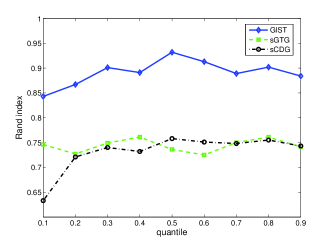
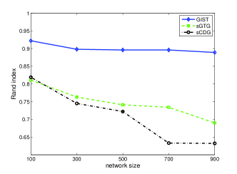
Given any network data, we apply GIST to obtain a JAG estimate and perform robust decomposition (cf. Section III-D). The decompositions of sole GTG (assuming $\boldsymbol{\hat{\Omega}}_{sGTG}=\boldsymbol{I}$) and sole CDG (assuming $\boldsymbol{\hat{B}}_{sCDG}=\boldsymbol{0}$ after centering the data) are obtained as well. All decompositions are via spectral clustering. Although GIST considers a more complex model, because of its screening nature, it runs efficiently. The mean RI results are shown in Figure 3.

In all the settings, GIST achieves more reliable decomposition and outperforms sGTG and sCDG by a large margin. This shows that the network decomposition based on the joint graph is trustworthy. Moreover, its performance is rather insensitive to the choice of the quantile parameter $q$ as long as $qp^{2}$ bounds the true network cardinality. This offers great ease in practice.

GIST is also superfast: for any network in the experiments, it just takes a few seconds to obtain the graphical screening pattern or subnetwork structure. A more comprehensive computational cost investigation is given in the next subsection.

(a) RI versus quantile ($p=500$)

(b) RI versus network size ($q=0.5$)

Figure 3: Rand index comparison on simulated networks consisting of two equally-sized subnetworks.

V-C Computation time reduction via graph screening

Now we study how much computational cost can be saved by applying GIST before fine learning. All simulated networks consist of multiple equally-sized subnetworks, with the total number of nodes denoted by $p$ and the number of nodes in each subnetwork denoted by $p_{s}$. The diagonal blocks of $\boldsymbol{B}$ and $\boldsymbol{\Omega}$ are generated in the same manner as in Section V-B. Let $T_{JGSE}$ be the total computation time of JGSE learning (“GIST+FLOG”), and $T_{FLOG}^{(w)}$ be the computation time by applying FLOG directly to the whole network without graph screening or decomposition. (We did not include MRCE in the comparison because it is extremely slow for large data). Solution paths of $\boldsymbol{B}$ and $\boldsymbol{\Omega}$ are computed for a grid of values for $(\lambda_{B},\lambda_{\Omega})$ that covers various sparsity patterns. The quantile parameter is set as 0.3 in GIST. We report the ratios $T_{JGSE}/T_{FLOG}^{(w)}$ for different combinations of ($p$, $p_{s}$) in Table II, where $n=100$ in all experiments.

Table II: Computation time reduction offered by JGSE on simulated networks, with $p$ denoting the total number of nodes and $p_{s}$ the number of nodes for each subnetwork.

$(p,p_{s})$	(500,250)	(500,100)	(500,50)	(1000,500)	(1000,200)	(1000,100)
$T_{JGSE}/T_{FLOG}^{(w)}$	0.427	0.161	0.133	0.404	0.148	0.112

Table II shows that at least half of the running time can be reduced when the network is decomposable. The larger the ratio $p/p_{s}$ is, the more computational cost can be saved. We conducted the experiment on a PC, but if parallel computing resources are available, the computational efficiency can be further boosted. The network decomposition technique makes an otherwise computationally expensive or even infeasible problem much easier to solve.

VI Applications

In this section, we analyze real data from $S\&P$ 500 and NASDAQ-100 stock using JGSE.

VI-A S&P 500

This dataset keeps a record of the closing prices of the $S\&P$ 500 stocks from Jan. 1, 2003 to Jan. 1, 2008. It consists of 1258 samples for 452 stocks. The data have been preprocessed by taking logarithm and differencing transformations [22].

We first applied GIST (with quantile $q=0.1$) and the robust JAG decomposition. Figure 4a shows the resulting clusters, where the nodes are placed by the Fruchterman-Reingold algorithm [44]. Although no ground truth is available, interestingly, we found that the obtained 10 subnetworks are highly consistent with the 10 given categories in the data documentation—the corresponding RI is almost as high as 0.9 (cf. Figure 4b).

(a) JAG decomposition ($q=0.1$).

(b) Rand index comparison.

Figure 4: GIST on $S\&P$ 500.

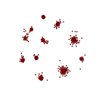
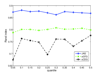
We then varied $q$ and systematically studied the clustering results based on GIST. The RIs with respect to the 10 stock categories are shown in Figure 4b. For comparison, sGTG and sCGD clusterings are also included. Our JAG decomposition is quite robust to the choice of $q$ in GIST. It seems that the 10-category structure in the documentation is reflected on the real stock data.

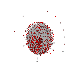
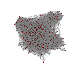
We also applied the popular BDSR [21, 20] (which is designed under the sole CDG learning setup), to decompose S&P 500 into 10 subnetworks. Figure 5a shows that the network is now decomposed into a giant cluster and nine isolated nodes, which is more difficult to interpret than GIST. Such a decomposition provides little help in reducing the computational cost. Furthermore, Figure 5b shows the best tuned sCDG estimate (using the R package huge [22] with default parameters) at $\lambda^{*}=0.08$. To achieve a 10-subnetwork decomposition, we found that $\lambda$ must be greater than or equal to $0.22$. This is the dilemma discussed in Section III-D: BDSR resorts to setting an overly large value for $\lambda$ to yield graph decomposition, while such a high thresholding level may mask many truly existing edges and result in an inaccurate estimate. Correspondingly, its decomposition structure is unreliable. Of course, the poor performance of BDSR also has a lot to do with the fact that the transition matrix or GTG estimation is ignored in the sCDG learning.

(a) Block diagonal screening

(b) Optimal sCDG estimate

Figure 5: Gaussian graph learning (or sCDG) on $S\&P$ 500.

We next investigate the forecasting capability of JGSE, by use of the conventional rolling MSE scheme (see, e.g., [45]). Denote the rolling window size as $W$. Standing at time point $t_{0}$, apply the estimation algorithm to the most recent $W$ observations in the past, i.e., $\{\boldsymbol{x}_{t}\}_{t=t_{0}-W+1}^{t_{0}}$. Then use the estimate $\boldsymbol{\hat{B}}_{t}$ to forecast $\boldsymbol{x}_{t+h}$: $\boldsymbol{\hat{x}}_{t+h}=\boldsymbol{\hat{B}}_{t}^{\mathsf{T}}\boldsymbol{\hat{x}}_{t+h-1}$ for $h\geq 1$, and $\boldsymbol{\hat{x}}_{t}\triangleq\boldsymbol{x}_{t}$. Repeat the forecasting procedure till the rolling window slides to the end of the time series. The rolling MSE is defined as $MSE=\frac{1}{n-h-W+1}\sum_{t=W}^{n-h}\|\boldsymbol{x}_{t+h}-\hat{\boldsymbol{x}}_{t+h}\|^{2}_{2}$. We set the window size $W=0.8n$ and horizon $h=1$ and compared sGTG, MRCE, and JGSE in each category. Because of the limited sample size, the large-data validation used in synthetic experiments is not applicable. Following [25, 46, 47], we chose the tuning parameters by BIC, where the number of degrees of freedom is given by $\sum_{i,j}1_{\hat{b}_{ij}\neq 0}+\sum_{i\leq j}1_{\hat{\omega}_{ij}\neq 0}$ if both $\boldsymbol{B}$ and $\boldsymbol{\Omega}$ are estimated, and $\sum_{i,j}1_{\hat{b}_{ij}\neq 0}$ if only $\boldsymbol{B}$ is estimated. Table III reports the rolling MSEs (times 1e+4 for better readability) for the first five categories. (The conclusions for the last five categories are similar but the first five have relatively larger dimensions.) Even compared with the widely acknowledged MRCE, JGSE offers better or comparable forecasting performance.

Table III: Rolling MSE comparison on S&P 500.

Model & Method	Category 1	Category 2	Category 3	Category 4	Category 5
sGTG	236.6	883.5	237.4	1859.1	456.5
MRCE	28.4	742.6	5.0	250.1	7.9
JGSE	1.4	3.7	2.0	5.4	7.9

VI-B NASDAQ-100

The NASDAQ-100 consists of 100 of the largest non-financial companies listed on the NASDAQ stock market. We collect the closing prices of the stocks for each trading day from Jan.1 , 2011 to Dec. 31, 2011, which gives 252 samples in total (the data is downloaded from finance.yahoo.com). Differencing is applied to remove trends. There were several significant changes to the indices during 2011. For example, NASDAQ rebalanced the index weights on May 2, 2011 before opening the market—see http://ir.nasdaqomx.com/releasedetail.cfm?releaseid=561718. More event details can be found at http://en.wikipedia.org/wiki/NASDAQ-100#Changes_in_2011. In consideration of such major changes, we focus on the following segments. Segment 1 consists of 62 samples from Jan. 1 to Apr. 4; Segment 2 consists of 23 samples from Apr. 4 to May 2; Segment 3 consists of 32 samples from May 31 to Jul. 14; and Segment 4 consists of 98 samples from Jul.15 to Dec. 2.

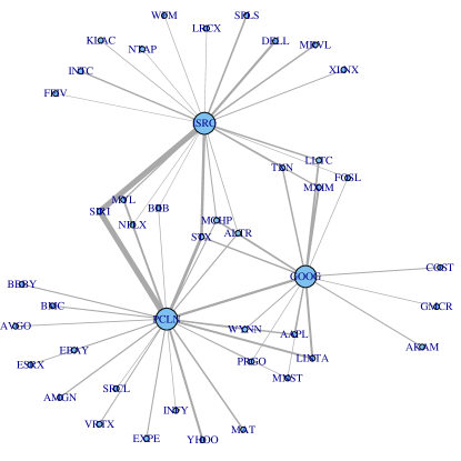
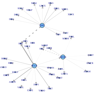
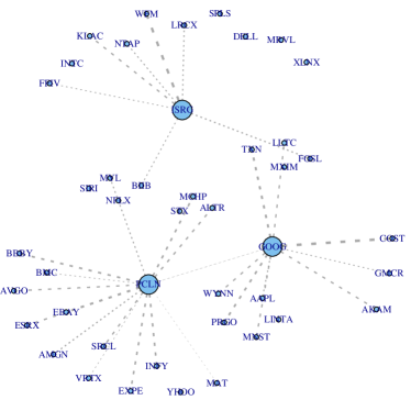
We present the analysis of Segment 4 as an example. To get a conservative idea of the network cardinality, we applied sGTG and sCDG to the data respectively. Sparse graphs are obtained with around $1\%$ connections. We set $q=0.02$ in running the GIST algorithm. After removing the isolated indices, we applied the FLOG algorithm to obtain the GTG and CDG estimates. The whole procedure only took a few minutes. We are particularly interested in the hub nodes in the JAG. Figure 6 shows all connections to and from the hub nodes. Nicely, the three hubs, PCLN (Priceline.com Inc.), GOOG (Google Inc.) and ISRG (Intuitive Surgical Inc.), come from the three largest sectors of the NASDAQ-100, namely Consumer Service, Technology and Health Care, respectively. PCLN is a commercial website that helps customers obtain discounts for travel-related purchases, and it is not surprising that PCLN is related to some companies providing similar services, such as EXPE (Expedia Inc.), and some hospitality companies such as WYNN (Wynn Resorts, Limited). Similarly, GOOG, as a world-famous technology company, is related to many technology based companies, such as AAPL (Apple Inc.), TXN (Texas Instruments Inc.), LLTC (Linear Technology Corporation) and so on. ISRG, a corporation that manufactures robotic surgical systems, is connected with INTC (Intel Corporation), MRVL (Marvell Technology Group Ltd.) and KLAC (KLA-Tencor Corporation), which all produce semiconductor chips and nanoelectronic products to be used in robotics.

The obtained GTG and CDG share some common connections. For example, PCLN not only has a negative causal influence over EXPE, but shows negatively correlation with it conditioned on the other nodes. On the other hand, the two graphs differ in some ways. For example, although PCLN strongly Granger-causes SIRI (Sirius XM Holdings, Inc.), they are conditionally independent. The interaction between LLTC and GOOG is of second order, purely due to their conditional dependence without any direct Granger causality. Fortunately, JAG encompasses all significant links on either GTG or CDG, and provides comprehensive network screening.

(a) JAG

(b) GTG

(c) CDG

Figure 6: The JAG, GTG and CDG of NASDAQ-100. The size of node is proportional to its degree. The edge width indicates the weight of the connection. Solid/dotted lines represent positive/negative weights.

We have performed similar analysis for other segments and examined the changes of the network topology. Due to page limitation, details are not reported here.

Next, we call the rolling scheme to investigate the forecasting performance of JGSE. For comparison, sGTG was also included; MRCE is however computationally intractable here, and so we applied our FLOG^w instead. BIC was used for regularization parameter tuning. The rolling MSEs of three methods are shown in Table IV, with window size $W=0.8n$ and horizon $h=1$. We see that the joint estimation by FLOG^w outperforms the popular transition estimation (sGTG) in three of the four segments. This suggests the existence of wide range conditional dependence between the stocks, and it is beneficial to take into account such correlations in statistics modeling. JGSE is able to further improve the forecasting performance by joint regularization, which is however not surprising from Stein et al.’s classical works (e.g., [8]). It also has a lot to do with the success of GIST in reducing the search space for the fine graph learning. These echo the findings in synthetic data experiments in Section V-A.

Table IV: Rolling MSE comparison on NASDAQ-100.

Model & Method	Segment 1	Segment 2	Segment 3	Segment 4
sGTG	24.3	30.8	20.6	32.2
FLOGw	21.9	31.4	20.1	18.4
JGSE	18.6	28.7	18.6	15.1

VII Conclusion

We studied large-scale dynamical networks with sparse first-order and second-order statistical structures, where the first-order connections can be captured by a directed Granger transition graph and the second-order correlations by an undirected conditional dependence graph. To jointly regularize the two graphs in topology identification and dynamics estimation, we proposed the 2-stage JGSE framework. The GIST algorithm was developed for JAG screening and decomposition. As demonstrated by extensive synthetic-data experiments and real-world applications, our proposed algorithms beat the commonly used BDSR and MRCE in graph decomposition and estimation.

References

- Sims [1980] C. A. Sims, “Macroeconomics and reality,” Econometrica, vol. 48, no. 1, pp. 1–48, Jan. 1980.
- Gourieroux and Jasiak [2002] C. Gourieroux and J. Jasiak, “Financial econometrics problems, models and methods,” University Presses of California, Columbia and Princeton: New Jersey, 2002.
- Fujita et al. [2007] A. Fujita, J. Sato, H. Garay-Malpartida, R. Yamaguchi, S. Miyano, M. Sogayar, and C. Ferreira, “Modeling gene expression regulatory networks with the sparse vector autoregressive model,” BMC Systems Biology, vol. 1, no. 1, 2007.
- Bullmore and Sporns [2009] E. Bullmore and O. Sporns, “Complex brain networks: graph theoretical analysis of structural and functional systems,” Nature Reviews Neuroscience, vol. 10, pp. 186–198, Mar. 2009.
- Granger [1969] C. W. J. Granger, “Investigating causal relations by econometric models and cross-spectral methods,” Econometrica, vol. 37, no. 3, pp. 424–438, 1969.
- He et al. [2013] Y. He, Y. She, and D. Wu, “Stationary sparse causality network learning,” J. Mach. Learn. Res., vol. 14, pp. 3073–3104, 2013.
- She et al. [2014] Y. She, Y. He, and D. Wu, “Learning topology and dynamics of large recurrent neural networks,” IEEE Transactions on Signal Processing, 2014, to appear.
- Stein [1956] C. Stein, “Inadmissibility of the usual estimator for the mean of a multivariate distribution,” Proc. Third Berkeley Symp. Math. Statist. Prob., vol. 1, pp. 197–206, 1956.
- Bolstad et al. [2011] A. Bolstad, B. D. Van Veen, and R. Nowak, “Causal network inference via group sparse regularization,” Signal Processing, IEEE Transactions on, vol. 59, no. 6, pp. 2628–2641, 2011.
- Valdes-Sosa [2005] P. A. Valdes-Sosa, “Estimating brain functional connectivity with sparse multivariate autoregression,” Phil. Trans. R. Soc. B, pp. 969–981, 2005.
- Banerjee et al. [2008] O. Banerjee, L. El Ghaoui, and A. d’Aspremont, “Model selection through sparse maximum likelihood estimation for multivariate gaussian or binary data,” The Journal of Machine Learning Research, vol. 9, pp. 485–516, 2008.
- Friedman et al. [2008] J. Friedman, T. Hastie, and R. Tibshirani, “Sparse inverse covariance estimation with the graphical lasso,” Biostatistics, vol. 9, no. 3, pp. 432–441, Jul. 2008.
- Bickel and Levina [2008] J. Bickel and E. Levina, “Regularized estimation of large covariance matrices,” Ann. Statist, vol. 36, no. 1, pp. 199–227, 2008.
- Meinshausen and Bühlmann [2006] N. Meinshausen and P. Bühlmann, “High-dimensional graphs and variable selection with the lasso,” The Annals of Statistics, vol. 34, no. 3, pp. 1436–1462, 2006.
- Rothman et al. [2010] A. J. Rothman, E. Levina, and J. Zhu, “Sparse multivariate regression with covariance estimation,” Journal of Computational and Graphical Statistics, vol. 19, no. 4, 2010.
- Lee and Liu [2012] W. Lee and Y. Liu, “Simultaneous multiple response regression and inverse covariance matrix estimation via penalized gaussian maximum likelihood,” Journal of Multivariate Analysis, 2012.
- James and Stein [1961] W. James and C. Stein, “Estimation with quadratic loss,” Berkeley, Calif., pp. 361–379, 1961.
- Fink et al. [2009] A. Fink, R. H. Grabner, M. Benedek, G. Reishofer, V. Hauswirth, M. Fally, C. Neuper, F. Ebner, and A. C. Neubauer, “The creative brain: Investigation of brain activity during creative problem solving by means of eeg and fmri,” Human Brain Mapping, vol. 30, no. 3, pp. 734–748, 2009.
- Stock and Watson [2012] J. H. Stock and M. W. Watson, “Generalized shrinkage methods for forecasting using many predictors,” Journal of Business & Economic Statistics, vol. 30, no. 4, pp. 481–493, 2012.
- Witten et al. [2011] D. M. Witten, J. H. Friedman, and N. Simon, “New insights and faster computations for the graphical lasso,” Journal of Computational and Graphical Statistics, vol. 20, no. 4, pp. 892–900, 2011.
- Mazumder and Hastie [2012] R. Mazumder and T. Hastie, “Exact covariance thresholding into connected components for large-scale graphical lasso,” J. Mach. Learn. Res., vol. 13, pp. 781–794, Mar. 2012.
- Zhao et al. [2012] T. Zhao, H. Liu, K. Roeder, J. Lafferty, and L. Wasserman, “The huge package for high-dimensional undirected graph estimation in r,” J. Mach. Learn. Res., vol. 13, no. 12, pp. 1059–1062, Jun. 2012.
- Lütkepohl [2007] H. Lütkepohl, New Introduction to Multiple Time Series Analysis, 1st ed. Springer, Oct. 2007.
- Tibshirani [1996] R. Tibshirani, “Regression shrinkage and selection via the lasso,” Journal of the Royal Statistical Society, vol. 58, no. 1, pp. 267–288, 1996.
- Yuan and Lin [2007] M. Yuan and Y. Lin, “Model selection and estimation in the gaussian graphical model,” Biometrika, vol. 94, no. 1, pp. 19–35, 2007.
- Efron and Morris [1973] B. Efron and C. Morris, “Stein’s estimation rule and its competitors–an empirical bayes approach,” Journal of the American Statistical Association, vol. 68, no. 341, pp. pp. 117–130, 1973.
- She [2009] Y. She, “Thresholding-based iterative selection procedures for model selection and shrinkage,” Electron. J. Statist, vol. 3, pp. 384–415, 2009.
- She [2012] ——, “An iterative algorithm for fitting nonconvex penalized generalized linear models with grouped predictors,” Computational Statistics and Data Analysis, vol. 9, pp. 2976–2990, 2012.
- Fan and Li [2001] J. Fan and R. Li, “Variable selection via nonconcave penalized likelihood and its oracle properties,” Journal of the American Statistical Association, vol. 96, pp. 1348–1360, Dec. 2001.
- She et al. [2013] Y. She, H. Li, J. Wang, and D. Wu, “Grouped iterative spectrum thresholding for super-resolution sparse spectrum selection,” IEEE Transactions on Signal Processing, vol. 61, pp. 6371–6386, 2013.
- She [2013] Y. She, “Reduced rank vector generalized linear models for feature extraction,” Statistics and Its Interface, vol. 6, pp. 197–209, 2013.
- [32] ——, “Selectable factor extraction in high dimensions,” arXiv:1403.6212.
- Armijo [1966] L. Armijo, “Minimization of functions having Lipschitz continuous first partial derivatives,” Pacific Journal of Mathematics, vol. 16, no. 1, pp. 1–3, 1966.
- Duchi et al. [2008] J. Duchi, S. Gould, and D. Koller, “Projected subgradient methods for learning sparse Gaussians,” in Proceedings of the Twenty-fourth Conference on Uncertainty in AI (UAI), 2008.
- Dulmage and Mendelsohn [1958] A. L. Dulmage and N. S. Mendelsohn, “Coverings of bipartite graphs,” Canadian Journal of Mathematics, vol. 10, no. 4, pp. 516–534, 1958.
- von Luxburg [2007] U. von Luxburg, “A tutorial on spectral clustering,” Statistics and Computing, vol. 17, no. 4, pp. 395–416, 2007.
- von Luxburg et al. [2008] U. von Luxburg, M. Belkin, and O. Bousquet, “Consistency of spectral clustering,” The Annals of Statistics, pp. 555–586, 2008.
- Fraley and Raftery [1998] C. Fraley and A. E. Raftery, “How many clusters? which clustering method? answers via model-based cluster analysis,” The Computer Journal, vol. 41, no. 8, pp. 578–588, 1998.
- Tibshirani et al. [2001] R. Tibshirani, G. Walther, and T. Hastie, “Estimating the number of clusters in a data set via the gap statistic,” Journal of the Royal Statistical Society: Series B (Statistical Methodology), vol. 63, no. 2, pp. 411–423, 2001.
- Sugar and James [2003] C. A. Sugar and G. M. James, “Finding the number of clusters in a dataset: An information-theoretic approach,” Journal of the American Statistical Association, vol. 98, no. 463, pp. 750–763, 2003.
- Nocedal and Wright [2006] J. Nocedal and S. J. Wright, Numerical Optimization, 2nd ed. New York: Springer, 2006.
- Friedman et al. [2007] J. Friedman, T. Hastie, H. Höfling, and R. Tibshirani, “Pathwise coordinate optimization,” The Annals of Applied Statistics, vol. 1, no. 2, pp. 302–332, 2007.
- Rand [1971] W. M. Rand, “Objective criteria for the evaluation of clustering methods,” Journal of the American Statistical Association, vol. 66, no. 336, pp. 846–850, 1971.
- Fruchterman and Reingold [1991] T. M. Fruchterman and E. M. Reingold, “Graph drawing by force-directed placement,” Software: Practice and experience, vol. 21, no. 11, pp. 1129–1164, 1991.
- Makridakis et al. [1998] Makridakis, Wheelwright, and Hyndman, Forecasting: Methods and Applications. Wiley, 1998.
- Yin and Li [2011] J. Yin and H. Li, “A sparse conditional gaussian graphical model for analysis of genetical genomics data,” The Annals of Applied Statistics, vol. 5, no. 4, p. 2630, 2011.
- Guo et al. [2011] J. Guo, E. Levina, G. Michailidis, and J. Zhu, “Joint estimation of multiple graphical models,” Biometrika, p. asq060, 2011.