Quantum criticality at the Anderson transition: a TMT perspective

Abstract

We present a complete analytical and numerical solution of the Typical Medium Theory (TMT) for the Anderson metal-insulator transition. This approach self-consistently calculates the typical amplitude of the electronic wave-functions, thus representing the conceptually simplest order-parameter theory for the Anderson transition. We identify all possible universality classes for the critical behavior, which can be found within such a mean-field approach. This provides insights into how interaction-induced renormalizations of the disorder potential may produce qualitative modifications of the critical behavior. We also formulate a simplified description of the leading critical behavior, thus obtaining an effective Landau theory for Anderson localization.

I Introduction

Many physical systems display puzzling features, which are often associated with the metal-insulator transition (MIT) Dobrosavljević et al. (2012). Although the important roles of both the Anderson Anderson (1958) (disorder-driven) and the Mott Mott (1990) (interaction-driven) routes to localization have been long appreciated, formulating a simple order-parameter theory describing their interplay has remained a challenge. Important advances have been achieved, over the last twenty years, with the development of Dynamical Mean Field Theory (DMFT) Georges et al. (1996) methods, which provided new insights into how such an order-parameter theory can be constructed. Although the original DMFT formulation adequately describes many features of strongly correlated electron systems, it proved unable to capture Anderson localization effects, which cannot be neglected in presence of sufficiently strong disorder Miranda and Dobrosavljevic (2005).

To overcome these limitations, DMFT was extended to describe spatially nonuniform systems, in approaches sometimes called “Statistical DMFT” Miranda and Dobrosavljevic (2005); Dobrosavljević and Kotliar (1997); Miranda and Dobrosavljević (2001); Aguiar et al. (2003); Song et al. (2008); Tran (2007); Song et al. (2009); Andrade et al. (2009); Semmler et al. (2010a, b); Semmler et al. (2011); Aguiar and Dobrosavljević (2013) (some authors call the same approach “Real-Space DMFT” Potthoff and Nolting (1999); Helmes et al. (2008); Snoek et al. (2008)). Here, the local DMFT order parameters (i.e. the appropriate local self-energies) are self-consistently calculated at each lattice site for a given realization of disorder, in a fashion similar to the Thouless-Anderson-Palmer (TAP) theory Thouless et al. (1977) for spin glasses. These efforts immediately produced a wealth of new information, discovering phenomena such as disorder-driven non-Fermi liquid behavior Miranda and Dobrosavljevic (2005) and the emergence of Electronic Griffiths Phases Andrade et al. (2009); Dobrosavljević et al. (2012) in the vicinity of the MIT. Despite these advances, progress has remained slow, primarily because such approaches typically require very large-scale numerical computations.

The missing key point in all these formulations was the lack of an appropriate local order parameter, which is capable of recognizing Anderson localization. A hint on how to overcome this difficulty was first provided in the seminal 1958 work by P. W. Anderson Anderson (1958), who emphasized that the typical (i.e. geometrically averaged) local density of states (TDOS) vanishes at the transition, in contrast to its algebraically averaged counterpart. This idea was later confirmed by large-scale computational studies M.Janssen (1998) of the wave-function amplitude statistics, which suggested that this quantity should play the role of an appropriate order-parameter for this problem.

A self-consistent calculation of TDOS was recently formulated, dubbed “Typical-Medium Theory” (TMT) Dobrosavljević et al. (2003), which can be regarded as the conceptually simplest order-parameter approach for Anderson localization. This method uses the same “cavity-field” construction as in standard DMFT methods Georges et al. (1996), and represents an elegant and effective approach to treat both the correlation and the localization effects on the same footing. Following its discovery in 2003, TMT was quickly applied to various problems with both interactions and disorder Byczuk et al. (2005); Aguiar et al. (2006); Byczuk et al. (2009); Aguiar et al. (2009); Aguiar and Dobrosavljević (2013); Oliveira et al. (2014), providing useful new information which would be difficult to obtain by alternative methods. The numerical solution of TMT equations has been obtained for both the (non-interacting) Anderson Dobrosavljević et al. (2003); Dobrosavljevic (2010), and the Mott-Anderson Byczuk et al. (2005); Aguiar et al. (2006, 2009); Byczuk et al. (2009); Oliveira et al. (2014) transition. However, deeper understanding of what one can generally expect from TMT approaches would require a complete analytical solution for the critical behavior, which has not been available so far.

Further motivation for our work is found in recent experiments that were able to visualize the electronic wave function near the metal-insulator transition, via scanning tunneling microscopy on $\mathrm{Ga_{1-x}Mn_{x}As}$ Richardella et al. (2010). This work highlighted the crucial importance of the long-range Coulomb interaction, and confirmed the early theoretical prediction of Efros and Shklovskii (ES) Efros and Shklovskii (1975); Efros (1976), that Coulomb interactions lead to the formation of a pseudogap within the insulating phase. Within the ES picture, the gap opening is produced by the electrostatic shifts of the (random) site energies, resulting in a significantly renormalized probability distribution for the effective random potential seen by the electrons. While the ES mechanism is by now well documented by both theoretical and experimental studies on the insulating side of the MIT Efros and Pollak (1985), its precise role for the critical region has remained elusive. At the minimum, one should investigate the effects of such pseudo-gap opening in the form of the distribution function for disorder, and its role at the Anderson transition.

In this paper, we address and clearly answer the following physical questions: (1) What types of quantum criticality can be found, for the noninteracting Anderson localization transition, within the TMT scheme, and how does the result depend on the model dependent details of the band structure (e.g. particle-hole symmetry)? (2) How is the critical behavior modified in cases where the renormalized disorder distribution assumes a pseudo-gap form predicted by the ES theory? We accomplish this by first presenting a detailed numerical solution of the TMT equation, for several cases of relevance. We then obtain a full analytical solution of the TMT equation, describing the leading critical behavior which is in complete agreement with the numerics, and includes the emergence of logarithmic corrections to scaling. This insight is shown to provide a new perspective and a simple physical understanding of several puzzling features of the critical behavior, previously observed in both numerical studies and in experiments.

The rest of the paper is organized as follows. In section II we present the general formulation of Typical-Medium Theory, and provide some illustrative examples of relevance to experiments. We show that two distinct types of critical behavior can be found within TMT, and investigate their main features. A general strategy to analytically solve the critical behavior within TMT is discussed in Section III, based on an expansion in powers of order parameter (TDOS). We explain why a simple solution can be obtained only in the special case of particle-hole symmetry, which already provides a classification of possible types of quantum criticality within TMT. We further investigate how it is affected by the form of distribution of random site energies. In section IV we present a detailed analytical solution for the leading critical behavior in absence of particle-hole symmetry, by reducing the problem to a close-form solution of an appropriate Fredholm integral equation. We show that particle-hole asymmetry leads to the emergence of logarithmic corrections to scaling, leading to a (mild) modification of the critical behavior at the mobility edge away from the band center. Finally, based on our full understanding of the mathematical structure of the theory, we present a simplified Landau theory for Anderson localization in Section V. This approximation ignores the relatively mild logarithmic corrections, but is still shown to capture all the important qualitative trends of the full TMT solution, and to reproduce most of the qualitative features observed in the large-scale numerics, as well as in some experiments.

II Model and numerical solution of TMT equations

The general strategy in formulating a local order-parameter theory such as TMT follows the “cavity” method typically used in Dynamical Mean Field Theory approaches Georges et al. (1996). Here, the dynamics of an electron on a given site can be obtained by integrating out all the other sites, and replacing its environment by an appropriately averaged “effective medium” characterized by a local self energy $\Sigma(\omega)$. This method can be utilized to self-consistently calculate any desired local quantity, and in the following we briefly review its application to TMT of Anderson localization Dobrosavljević et al. (2003); Dobrosavljevic (2010). For simplicity, we concentrate on a single band tight binding model of non-interacting electrons with random site energies $\epsilon_{i}$ with a given distribution $P(\epsilon_{i})$, which the Hamiltonian of this system can be written as:

$$H=\sum_{\left\langle ij\right\rangle,\sigma}t_{ij}c_{i\sigma}^{\dagger}c_{j\sigma}+\sum_{i,\sigma}\varepsilon_{i}c_{i\sigma}^{\dagger}c_{i\sigma}.$$ (1)

Here, $c_{i\sigma}^{\dagger}$ and $c_{i\sigma}$ are the electron creation and annihilation operators, and $t_{ij}$ are the inter-site hopping elements. The local (retarded) Green function corresponding to site $i$ can be written as

$$G_{ii}(\omega,\epsilon_{i})=[\omega+i\eta-\epsilon_{i}-\Delta(\omega)]^{-1},$$ (2)

where the “cavity field” $\Delta(\omega)$ represents the effective medium, i.e. available electronic states to which an electron can hop from of a given lattice site. It is defined by incorporating the local self-energy $\Sigma(\omega)$ as

$$\Delta(\omega)=\Delta_{0}(\omega-\Sigma(\omega)),$$ (3)

where $\Delta_{0}(\omega)$ is the “bare” (corresponding to zero disorder) cavity field Georges et al. (1996). It can be obtained from the bare lattice Green’s function through relation

$$\Delta_{0}(\omega)=\omega-\frac{1}{G_{0}(\omega)},$$ (4)

and the bare lattice Green’s function

$$G_{0}(\omega)=\int_{-\infty}^{+\infty}d\omega^{\prime}\frac{\nu_{0}(\omega^{\prime})}{\omega+i\eta-\omega^{\prime}}.$$ (5)

is given by the Hilbert transform of the bare density of states $\nu_{0}(\omega)$ (DOS), which specifies the electronic band structure for a given lattice. The corresponding local density of states (LDOS) is given by the imaginary part of the local Green’s function:

$$\rho_{i}(\omega,\epsilon_{i})=-\frac{1}{\pi}\mathrm{Im}G_{ii}(\omega,\epsilon_{i}).$$ (6)

Within the effective-medium approximation we consider, this local quantity displays site-to-site fluctuations. Due to its dependence on the local site energy $\epsilon_{i}$, it reflects the spatial fluctuations of the local wave-function amplitudes $\rho_{i}\sim|\psi_{i}|^{2}$. To properly define the effective medium, one has to perform an appropriate spatial average, in order to close the self-consistency loop. The simplest choice is to consider its algebraic average (ADOS)

$$\rho_{avg}(\omega)=\int d\epsilon_{i}P(\epsilon_{i})\rho_{i}(\omega,\epsilon_{i})$$ (7)

as the appropriate order parameter, and this leads to the well-known coherent-potential approximation (CPA) Economou (2006), which unfortunately fails to capture Anderson localization.

In the presence of strong disorder, however, LDOS displays strong spatial fluctuations and is very broadly distributed. As a result, its typical (i.e., most probable) value is ill-represented Anderson (1958) by the algebraic average $\rho_{avg}(\omega)$. Since the average density of states can remain finite throughout the insulating phase (even in the atomic limit) as well as in the metallic phase, it cannot distinguish between the phases. Therefore, within TMT, we introduce the typical value of the local density-of-states, as an appropriate order parameter. The statistic of LDOS reflects the degree of localization of quantum wave functions, and its typical value (TDOS) is known M.Janssen (1998) to be well-represented by the geometric average

$$\rho_{typ}(\omega)=\exp\left[\int d\epsilon_{i}P(\epsilon_{i})\ln\rho_{i}(\omega,\epsilon_{i})\right].$$ (8)

Indeed, large-scale computational studies, as well as the available analytical results in $d=2+\varepsilon$ dimensions , demonstrated that TDOS vanishes in a power-law fashion at the critical point, and also displays the appropriate finite-size scaling behavior (for reviews see Refs. M.Janssen (1998); Evers and Mirlin (2008)). These results strongly suggest M.Janssen (1998) that TDOS should be chosen as an appropriate local order parameter; its self-consistent calculation can be viewed as the conceptually simplest order-parameter theory of Anderson localization. In order to obey causality, the corresponding “typical” Green’s function, is defined Dobrosavljević et al. (2003); Dobrosavljevic (2010) by performing the Hilbert transform

$$G_{typ}(\omega)=\int_{-\infty}^{\infty}d\omega^{\prime}\frac{\rho_{typ}(\omega^{\prime})}{\omega+i\eta-\omega^{\prime}}.$$ (9)

Note that the $G_{typ}(\omega)$ has to be defined on the real frequency axis, because this is computed where LDOS is defined as a positive definite quantity and has a well-defined geometric average. Finally, we close the self-consistency loop by setting the Green functions of the effective medium to be equal to that corresponding to the local order parameter Dobrosavljević et al. (2003); Dobrosavljevic (2010),

$$G_{typ}(\omega)\equiv G_{0}(\omega-\Sigma(\omega)).$$ (10)

From this self-consistency condition and Eq. (4), we obtain the following equation which determines the self-energy of the system

$$G_{typ}(\omega)=[\omega+i\eta-\Sigma(\omega+i\eta)-\Delta(\omega+i\eta)]^{-1}.$$ (11)

It is important to emphasize that our procedure defined by TMT self-consistent equations (2-11) is not specific to the problem at hand; the same strategy is used in any mean-field (DMFT-like) theory characterized by a local self-energy Georges et al. (1996). The only requirement specific to TMT is the choice of the typical (geometrically-averaged) LDOS as the local order parameter. In other words, the only crucial difference between CPA and TMT is the fact that TMT utilizes the appropriate order parameter for Anderson localization.

This set of TMT self-consistent equations can be solved numerically for any specific lattice model, or any form of the random site energy distribution. However, as in any other mean-field formulation, only a limited number of qualitatively distinct types of critical behavior (i.e., universality classes) can arise, and in the following we discuss two distinct situations that we have found within TMT. Previous work mostly focused on models with continuous (e.g., uniform) distributions of site energies, and even some analytical results were obtain in this case Dobrosavljević et al. (2003).

In the following, we present the results obtained numerically by solving the TMT equations for semi-circular DOS which is given by $\nu_{0}(\omega)=2\sqrt{1-\omega^{2}}/\pi$. Here and in the the rest of the paper, all energies are expressed in units of the half-bandwidth. As an example, we consider the uniform model where the distribution of random site energies is continuous and is given by $P_{uniform}(\epsilon_{i})\equiv\frac{1}{W},$ over the interval $-\frac{W}{2}\leqslant\epsilon_{i}\leqslant\frac{W}{2}$. We display the resulting behavior for this model Dobrosavljević et al. (2003) in Fig. 1, showing the evolution of $\rho_{typ}(\omega)$ as disorder increases. The extended states are identified by the frequency range where $\rho_{typ}>0,$ which is seen to shrink and eventually disappear at a critical disorder $W=W_{c},$ where the entire band localizes. The metallic phase is separated from the Anderson insulator insulating phase by the mobility edge trajectory $\omega=\omega_{c}(W)$, corresponding to TDOS vanishing.

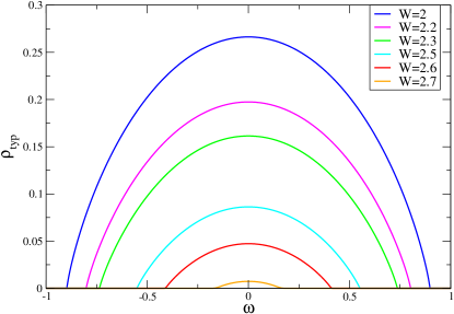
(a)

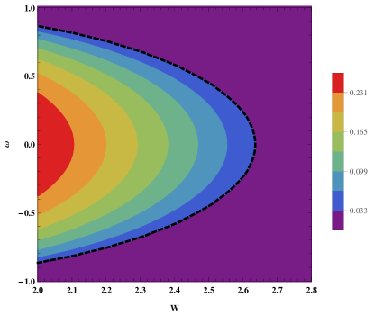
(b)

Figure 1: Evolution of the order parameter $\rho_{typ}(\omega)$ with increasing disorder for uniform model: $\rho_{typ}(\omega)$for several values of the disorder strength (top panel). The bottom panel shows the phase diagram in the $\omega-W$ plane, where the mobility edge (black dashed line) separates the extended states ($\rho_{typ}>0$) from the localized states ($\rho_{typ}=0$), and $\rho_{typ}$ is color coded.

The situation is qualitatively different if the disorder distribution has a gap or a pseudo-gap, so that $P(\epsilon)$ vanishes at one energy or in an entire energy interval. This situation can arise for discrete (e.g., binary) distributions of disorder, which can be found in alloys. A similar situation can also arise in presence of electron-electron interactions which we briefly discuss in the following. Here, the effective disorder potential (i.e., the renormalized random potential) seen by quasi-particles can be significantly modified by interaction effects, especially in presence of long-range Coulomb interactions, which leads to the formation of the soft “Coulomb gap” (pseudo-gap) at the Fermi energy. This behavior, which was recently brought to attention by scanning tunneling microscopy (STM) experiments Richardella et al. (2010) on $\mathrm{Ga_{1-x}Mn_{x}As}$, has been first discussed in the well-known theoretical work of Efros and Shklovskii (ES) Efros and Shklovskii (1975); Efros (1976); Efros and Pollak (1985). These authors argued that the key effect of the long-range Coulomb interactions is to provide a strong renormalizations of the electronic on-site energies, due to the fluctuating electrostatic potential produced by distant charges. Therefore, the renormalized site energy $\tilde{\varepsilon}_{i}$ is given by

$$\tilde{\varepsilon}_{i}=\varepsilon_{i}+e^{2}\sum_{j}\frac{n_{j}}{R_{ij}},$$ (12)

where $\tilde{\varepsilon}_{i}$ is the renormalized site energy, $n_{j}=0,1$ is the occupation number of a given lattice site $j$, $e$ is the electron charge, and $R_{ij}$ is the distance between sites $i$ and $j$.

According to the ES theory, the main result of the Coulomb interactions is to produce a renormalized distribution of disorder, which (in spatial dimension $d$) assumes a low-energy pseudo-gap form (vanishes in power-law fashion)

$$P(\tilde{\varepsilon})\sim\tilde{\varepsilon}^{d-2},$$ (13)

where the renormalized energy $\tilde{\varepsilon}_{i}$ is measured with respect to the Fermi energy. In other words, the renormalized distribution function vanishes at the Fermi energy, i.e., $P(0)=0,$ a situation which, as we shall see, leads to qualitatively different critical behavior of TDOS within TMT. The ES result was derived using a classical electrostatic model, which should be sufficient deep in the Anderson-localized phase. Closer to the MIT, the precise form of $P(\tilde{\varepsilon})$ may be affected by quantum fluctuations, as argued in Ref. Massey and Lee (1996), and it may need to be self-consistently calculated, in order to accurately capture the interplay of Anderson localization and the effects of the Coulomb interactions. Such a calculation may be possible within the framework of a DMFT-like formulation, by combining TMT with the EDMFT approach to Coulomb correlations Pramudya et al. (2011), but this rather complicated analysis is left as a challenge for future work.

In this paper, we limit our attention to analyzing, within TMT, the consequences of having such a pseudo-gap form for the disorder distribution function. As an illustration, we consider a model distribution of random site energies which assumes a pseudo-gap form expected from the ES picture in three dimensions:

$$P_{pseudo}(\tilde{\varepsilon}_{i})\equiv\frac{1}{(\frac{W}{6})^{3}\sqrt{2\pi}}\tilde{\varepsilon}_{i}^{2}\exp(-\frac{\tilde{\varepsilon}_{i}^{2}}{2(\frac{W}{6})^{2}}),$$ (14)

which we will refer as pseudo-gap model in the following text. We solved the TMT equations for this model of disorder, and the results for $\rho_{typ}(\omega)$ and $\rho_{avg}(\omega)$ are presented in Figs. 2 and 3. As disorder increases, the TDOS order parameter displays the most pronounced decrease precisely at the Fermi energy (here chosen at $\omega=0$); the corresponding electronic state is the one to first localize at the critical disorder strength $W_{c1}=2.07$. As disorder increases further, there emerges a finite “mobility gap” around the Fermi energy, where our TDOS order parameter $\rho_{typ}$ vanishes at $|\omega|<\omega_{c}(W)$, and all the electronic states within this region become localized. At even larger disorder $W=W_{c2}$ the entire band localizes. The trajectories of the corresponding mobility edges (shown by a dashed black line in Fig. 2(b)) displays the same non-monotonic behavior as found in the recent large-scale numerical study of the localization transition in Coulomb glasses Amini et al. (2014).

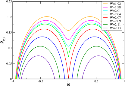
(a)

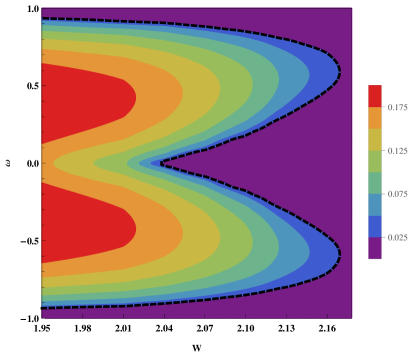
(b)

Figure 2: Evolution of the order parameter $\rho_{typ}(\omega)$ with increasing disorder for pseudo-gap model: $\rho_{typ}(\omega)$ for several disorder strength (top panel). The electronic states near the Fermi energy ($\omega=0$) are localized before the rest of the band would be localized.

For comparison with experiments, we also computed the algebraically-averaged local density of states (ADOS), which shows very different behavior. ADOS at the Fermi energy ($\omega=0$ ) is found to vanish at precisely the same critical disorder $W=W_{c1}$ for localization Richardella et al. (2010), but it remains finite at all other energies ($|\omega|>0$) within the localized phase, as shown in Fig. 3(b). Since we found that TDOS vanishes for $W>W_{c1}$ and $|\omega|<\omega_{c}(W)$ in Fig. 3(a), our numerical results immediately reveal that, within the entire localized phase, ADOS assumes a power-law low energy form

$$\rho_{avg}(\omega)\sim\omega^{2}.$$ (15)

In order to analytically understand this result, note that from Eq. (7), ADOS can be expressed as:

$$\rho_{avg}(\omega)=\frac{1}{\pi}\int d\epsilon P(\epsilon)\frac{\Delta^{\prime\prime}(\omega)}{(\omega-\varepsilon-\Delta^{\prime}(\omega))^{2}+\Delta^{\prime\prime}(\omega)^{2}}.$$ (16)

At $W>W_{c1}$ the imaginary part of the cavity field also vanishes at region $|\omega|<\omega_{c}(W),$ since it behaves as $\Delta^{\prime\prime}\sim\rho_{typ}$ (See appendix A). As it can be proven straightforwardly and is also shown numerically, the real part of the cavity field is a linear function as $\Delta^{\prime}(\omega)=A\omega$ with $A$ a finite constant, and we find

$$\rho_{avg}(\omega) = \frac{1}{\pi}\lim_{\Delta^{\prime\prime}\rightarrow 0}\{\int d\epsilon P(\epsilon)\frac{\Delta^{\prime\prime}}{((1-A)\omega-\varepsilon)^{2}+\Delta^{\prime\prime 2}}\}$$

$$= P((1-A)\omega)\sim P(\omega)\sim\omega^{2},$$

in agreement with ES theory.

Our results thus provide a qualitative picture of pseudo-gap formation of $\rho_{avg}(\omega)$, which is centered at $\omega=0$ both at the critical point $(W=W_{c1})$ and in the entire insulating phase ($W>W_{c1}$). This result (also shown in Fig. 3(b)) is consistent with large-scale exact diagonalization results Amini et al. (2014), and the available experimental findings Massey and Lee (1996); Richardella et al. (2010).

The emergence of qualitative different critical behavior, for the two distinct models of disorder, is even more clearly seen by examining our order parameter $\rho_{typ}$ at the center of the band $(\omega=0)$. Fig. 4 (top panel) shows that for pseudo-gap model $\rho_{typ}$ vanishes as square root of distance from transition viz. $\rho_{typ}\sim(W_{c1}-W)^{\frac{1}{2}}$, while for the uniform model (Fig. 4 bottom panel) we find linear behavior viz. $\rho_{typ}\sim(W_{c}-W)$. In order to try and understand the origin of these differences, in Section III we analytically recover the same critical behaviors at the band center $(\omega=0)$. Although this result gives us insight into the important differences between the two models, away from the band center this behavior cannot be explained in a simple way. This fact has been identified in previous workDobrosavljevic (2010); it has so far remained ill-understood, and clarifying this issue is the subject of our complete analytical solution in Sec. IV.

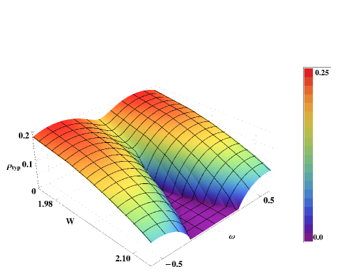
(a)

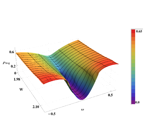
(b)

Figure 3: The evolution of the (a) typical and (b) average density of states for pseudo-gap model.

III Analytical solution: the Landau expansion

It is well known that the Anderson transition is a second-order phase transition, where the order parameter $\rho_{typ}(\omega)$ vanishes continuously as the transition is approached, as also confirmed by our numerical solution of the TMT equations. Using the fact that $\rho_{typ}(\omega)$ is infinitesimally small in the close vicinity of the transition, we can proceed as in deriving any Landau theory, by directly expand the TMT equations in the powers of the order parameter. For the sake of simplicity in notation we define

$$\rho_{typ}(\omega)\equiv\varphi(\omega).$$ (17)

The Anderson transition is found along the critical (mobility edge) line on the phase diagram, defined by the expression

$$\varphi[\omega_{c}(W)]=0,$$ (18)

as shown by a black dashed line in Fig. 1(b) and Fig. 2(b).

In order to obtain the solution as the transition is approached, we start with the general expression for TDOS, as given by Eq.(8), Eq.(6), and Eq.(2), which can be rewritten as

$$\pi\varphi(\omega)=\Delta^{\prime\prime}(\omega)g(\Delta^{\prime\prime}(\omega),\Delta^{\prime}(\omega)),$$ (19)

where,

$$g(\Delta^{\prime\prime}(\omega),\Delta^{\prime}(\omega)) \equiv \exp\{-\int d\epsilon P(\epsilon)$$

$$\times\log[(\omega-\epsilon-\Delta^{\prime}(\omega))^{2}+\Delta^{\prime\prime}(\omega)^{2}]\}.$$

To proceed, we note that near the mobility edge, where $\varphi\ll 1,$ the imaginary part of the cavity field is also small $(\Delta^{\prime\prime}\ll 1)$, since to leading order Dobrosavljević et al. (2003)

$$\Delta^{\prime\prime}=C\pi\varphi,$$ (20)

where $C=\int d\omega^{\prime}\omega^{\prime 2}\nu_{0}(\omega^{\prime})$, and $\nu_{0}(\omega)$ is a bare density of states (See Appendix A). In contrast, $\Delta^{\prime}(\omega_{c})$ generally remains finite. Indeed, we checked numerically that all qualitative features of the critical behavior do not depend on the specific choice of band structure Dobrosavljević et al. (2003), which only modifies the precise value of the prefactor $C$ in Eq.(20), and other non-universal quantities. We can, therefore, expand the right hand side of Eq.(19) in terms of $\varphi\sim\Delta^{\prime\prime}$, giving us a Landau-type expansion of the form

$$\frac{1}{C}=[a(\omega)+b(\omega)\varphi+d(\omega)\varphi{}^{2}+...].$$ (21)

Here,

$$a(\omega)\equiv\exp\{-2\int P(\epsilon)d\epsilon\log\mid\omega-\epsilon-\Delta^{\prime}(\omega)\mid\},$$ (22)

$$b(\omega)=-2\pi^{2}a(\omega)P(\omega-\Delta^{\prime}(\omega)),$$ (23)

$$d(\omega)=a(\omega)(\eta\pi^{2}+2\pi^{4}P(\omega-\Delta^{\prime}(\omega))^{2}),$$ (24)

and

$$\eta=\lim_{\Delta^{\prime\prime}\rightarrow 0}\{\int d\epsilon P(\epsilon)\frac{(\Delta^{\prime\prime}{}^{2}-\left(\omega-\epsilon-\Delta^{\prime}(\omega)\right)^{2})}{(\left(\omega-\epsilon-\Delta^{\prime}(\omega)\right)^{2}+\Delta^{\prime\prime}{}^{2})^{2}}\},$$ (25)

where $\eta$ remains finite for the models we examined.

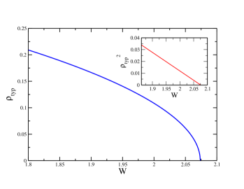
(a)

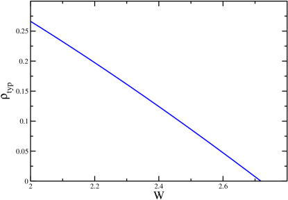
(b)

Figure 4: Critical behavior of TDOS as a function of disorder strength $W$ at half-filling ($\omega=0$), for (a) the pseudo-gap model, and (b) the uniform model of random site energies.

III.1 General critical behavior

As in any Landau theory, we can now directly obtain the critical behavior of the order parameter $\varphi(\omega)$, in terms of the coefficients in the expansion. For simplicity, consider a simple model band structure with semi-circular DOS where $C=1$, and solve the Eq. (21) for the order parameter $\varphi(\omega)$. For the generic model (e.g. uniform distribution of disorder) where $b(\omega_{c})\neq 0$, the leading critical behavior of typical density of states takes the form

$$\varphi(\omega)=\frac{1-\frac{1}{a(\omega)}}{2\pi^{2}P(\omega-\Delta^{\prime}(\omega))},$$ (26)

In contrast, whenever $b(\omega_{c})=0$ (e.g. the pseudo-gap model), we find

$$\varphi(\omega)=(\frac{\frac{1}{a(\omega)}-1}{\eta\pi^{2}})^{\frac{1}{2}},$$ (27)

At first glance, it seems that the critical behavior can be obtained easily given the cavity field, which is the functional of order parameter $\varphi(\omega),$ as $\Delta(\omega)=\mathcal{F}[\varphi(\omega)].$ However, the analytical solution is very complicated because the real part of the cavity field $\Delta^{\prime}(\omega)$ is an unknown function of $\omega$ which is linked to imaginary part $\Delta^{\prime\prime}(\omega)$ by the Hilbert transform. Thus, it is impossible to solve these equations analytically over a broad frequency range. As it has been shown numerically, we claim that this unknown function is finite near the mobility edge $(\omega\approx\omega_{c})$. In order to obtain the leading critical behavior of order parameter at transition, in in expression containing $P(\omega)$, we can replace

$$P(\omega-\Delta^{\prime}(\omega))\approx P(\omega_{c}-\Delta^{\prime}(\omega_{c})).$$ (28)

However, in other terms, e.g. in the expression for $a(\omega)$ (Eq. 22)), one needs to retain the full frequency dependence, which proves to assume a sufficiently singular form to contribute to leading order (see below). As a result, the critical behavior becomes a more complicated form, as we shall see from the full analytical solution of Eq.(21) close to the mobility edge. The specific form of the analytical solution has been provided in section IV for the two different classes of random distributions (uniform and pseudogap-gaussian), and it successfully has been compared with numerical results.

III.2 Critical behavior at half-filling

Here, we explore the exact functional form of order parameter close the transition, focusing on half-filling, where $\Delta^{\prime}(0)=0$. In this case, there is no need to perform the Hilbert transform, so all Landau coefficients can be evaluated in closed form a

$$a(0)=\exp\{-2\int P(\epsilon)d\epsilon\log\mid\epsilon\mid\}\equiv a,$$ (29)

and

$$b(0)=-2\pi^{2}P(0).$$ (30)

Our Landau-like expansion now takes simple form

$$1=a[1-2\pi^{2}P(0)\varphi+(\eta\pi^{2}+2\pi^{4}P(0){}^{2})\varphi^{2}+...].$$ (31)

Note that here the value of $P(0)$ plays an important role, and this what causes two different forms of criticality, for the generic model where $P(0)\neq 0$, and for the pseudo-gap model where $P(0)=0.$ For the generic case, the TDOS vanishes linearly at the transition

$$\varphi\sim(W-W_{c}),$$ (32)

while for models with $P(0)=0$, the critical behavior assumes a square-root form

$$\varphi\sim(W-W_{c1})^{\frac{1}{2}}.$$ (33)

We emphasize that the parameter $\eta$ remains finite at the transition, and can be directly calculated for any specific form for $P(\varepsilon)$ from Eq. (25). The condition $a=1$ directly gives us the critical value of disorder; for example, for the considered pseudo gap model we obtain $W_{c1}=2.07$, in excellent agreement with numerical results shown in Fig .4 (a) and Fig. 4(b).

IV FREDHOLM INTEGRAL EQUATION AND GENERAL SOLUTION

Here, we obtain the full analytical solution for the critical behavior, valid even away from particle hole symmetry, and for an arbitrary model of disorder.

IV.1 Analytical solution for a "generic model" with $b(\omega_{c})\neq 0$

The critical behavior of our TDOS order parameter, is given by Eq.(26), where it is expressed in terms of (the yet unknown) function $\Delta^{\prime}(\omega)$. Note, however, that (viz. Eq. 20) in the critical region $\varphi(\omega)\sim\Delta^{\prime\prime}(\omega)$ is linked through the Hilbert transform to $\Delta^{\prime}(\omega)$, since

$$\Delta^{\prime}(\omega)=H[\Delta^{\prime\prime}(\omega)].$$ (34)

Both quantities, therefore, need to be self-consistently calculated, as we do in the following. To do this, we express the all expressions in terms of $\Delta^{\prime\prime}(\omega)$; for simplicity we focus on the semi-circular band structure model where $C=1$, and we can write

$$\Delta^{\prime\prime}(\omega)=(1-\frac{1}{a(\omega)})\frac{1}{2\pi P(\omega-\Delta^{\prime}(\omega))}.$$ (35)

Using Eq. (28), to leading order we find

$$\Delta^{\prime\prime}(\omega)\approx\delta a(\omega)\frac{1}{2\pi P(\omega_{c}-\Delta^{\prime}(\omega_{c}))},$$ (36)

where $\delta a(\omega)\equiv(1-\frac{1}{a(\omega)})$ can be directly computed as a variation of $a(\omega)$ from Eq. (22) giving

$$\delta a(\omega)\approx 2\int d\epsilon P(\epsilon)\frac{1}{\omega-\epsilon-\Delta^{\prime}(\omega_{c})}(\delta\omega-\delta\Delta^{\prime}(\omega)).$$ (37)

Here, $\delta\omega\equiv\left|\omega-\omega_{c}\right|$ and $\delta\Delta^{\prime}(\omega)\equiv\Delta^{\prime}(\omega)-\Delta^{\prime}(\omega_{c})$. Using Eq.(36) we get the following integral equation linking $\Delta^{\prime}(\omega)$ and $\Delta^{\prime\prime}(\omega)$

$$\Delta^{\prime\prime}(\omega)=\varLambda_{0}(\delta\omega-\delta\Delta^{\prime}(\omega)).$$ (38)

Here, $\varLambda_{0}$ is a finite number, given by

$$\varLambda_{0}=\frac{1}{\pi P(\omega_{c}-\Delta^{\prime}(\omega_{c}))}\int d\epsilon\frac{P(\epsilon)}{\omega_{c}-\epsilon-\Delta^{\prime}(\omega_{c})}.$$ (39)

This result is valid for any (generic) model of disorder with $P(\omega_{c}-\Delta^{\prime}(\omega_{c}))\neq 0$. More explicitly, Eq.(38) can be rewritten as

$$\Delta^{\prime\prime}(\omega)-\frac{\varLambda_{0}}{\pi}\int_{-\infty}^{\infty}d\omega^{\prime}\frac{\Delta^{\prime\prime}(\omega^{\prime})}{\omega^{\prime}-\omega}=\varLambda_{0}(\delta\omega-\Delta^{\prime}(\omega_{c})).$$ (40)

This integral equation (40) can be recognized as the Fredholm Integral Equation (FIE), which assumes the form

$$y(x)-\lambda\int_{-\infty}^{\infty}dt\frac{y(t)}{t-x}=f(x).$$ (41)

By comparison of Eq.(40) and Eq.(41) it can be seen that in our case $y(x)=\Delta^{\prime\prime}(\omega)$, $\lambda=\frac{\varLambda_{0}}{\pi},$ and $f(x)=\varLambda_{0}(\delta\omega-\Delta^{\prime}(\omega_{c}))$. For completeness, we outline in the following the standard reasoning used in solving the FIE. It uses the fact that the Hilbert transform is a linear operator, with the additional property of being "idempotent", i.e. obeying and $H^{2}=-1$; this immediately gives us a hint how to solve it in closed form. We first apply the Hilbert transform on Eq.(41), and we can write

$$\frac{1}{\pi}\int_{-\infty}^{\infty}dt\frac{y(t)}{t-x}+\lambda\pi y(x)=H[f(x)].$$ (42)

Next, we use Eq.(41) and Eq.(42) to eliminatePolyanin and Manzhirov (2008) the term with the integral and express $y(x)$ entirely in terms of $f(x)$ giving

$$y(x)=\frac{1}{1+\pi^{2}\lambda^{2}}\left\{f(x)+\lambda\int_{-\infty}^{\infty}\frac{f(t)dt}{t-x}\right\}.$$ (43)

Applying this solution to our Eq.(40) we find

$$\Delta^{\prime\prime}(\omega)=\frac{\varLambda_{0}}{1+\varLambda_{0}^{2}}\delta\omega+\frac{\varLambda_{0}^{2}}{1+\varLambda_{0}^{2}}h(\frac{\delta\omega}{\omega_{0}}).$$ (44)

Here, $h(\frac{\delta\omega}{\omega_{0}})=H[1-\frac{\omega^{\prime}}{\omega_{0}}]$ is the Hilbert transform of $(1-\frac{\omega^{\prime}}{\omega_{0}})$ over the range where the (leading order, linear) approximation in Eq. (38) is valid, and it can be written as follows with $\omega_{0}$ as the cut-off of the limited frequency range:

$$h(\frac{\delta\omega}{\omega_{0}})=\frac{1}{\pi}\left\{\log\mid\frac{1+\frac{\delta\omega}{\omega_{0}}}{1-\frac{\delta\omega}{\omega_{0}}}\mid+\frac{\delta\omega}{\omega_{0}}\log\mid\frac{(\frac{\delta\omega}{\omega_{0}})^{2}-1}{(\frac{\delta\omega}{\omega_{0}})^{2}}\mid\right\}.$$ (45)

As mentioned before, this solution does not depend on the form of the disorder distribution function, other than through the value of the parameters $\frac{\varLambda_{0}}{1+\varLambda_{0}^{2}}$ and $\frac{\varLambda_{0}^{2}}{1+\varLambda_{0}^{2}}.$ As $\omega\rightarrow\omega_{c}$, these quantities can be estimated simply as $\frac{\varLambda_{0}}{1+\varLambda_{0}^{2}}\sim\omega_{c}-\Delta^{\prime}(\omega_{c})$ and $\frac{\varLambda_{0}^{2}}{1+\varLambda_{0}^{2}}\sim 1.$ This condition can be satisfied for both the pseudogap and the uniform model close to the mobility edge. Therefore, in this limit, from the Eq.(44) and Eq.(45) we find

$$\Delta^{\prime\prime}(\omega)\sim\varphi(\omega)\sim\left(\omega_{c}-\Delta^{\prime}(\omega_{c})+\frac{2}{\pi\omega_{0}}\right)\delta\omega-\frac{2}{\pi}\frac{\delta\omega}{\omega_{0}}\log\frac{\delta\omega}{\omega_{0}}.$$ (46)

Remarkably, we identified logarithmic corrections to the (linear) scaling behavior near the Anderson metal insulator transition, obtained with TMT theory. As we show in Section V, these non analytic corrections, however, are sufficiently mild to allow for a simplified theory to be formulated by neglecting them, without sacrificing the main quantitative prediction of full TMT.

IV.2 Analytical solution at the emergence of the pseudogap

Here, we obtain the critical behavior of $\rho_{typ}(\omega)$ as the pseudo-gap opens at $W=W_{c1}$. In this case the form of the disorder distribution prohibits us using Eq. (26) because $b(\omega_{c})=0$; we need to retain the terms to second order in $\Delta^{\prime\prime}$, in the expansion of Eq. (21). Therefore, from the Eq.(27) and Eq.(25) the imaginary part of the cavity field is expressed as

$$\frac{\Delta^{\prime\prime}(\omega)^{2}}{(\frac{W_{c1}}{6})^{2}}=(1-\frac{1}{a(\omega)})=\delta a(\omega).$$ (47)

Since we are interested in the behavior of the system at $W=W_{c1},$ we directly evaluate Eq.(37) as

$$\delta a(\omega) \approx 2\left(\omega-\Delta^{\prime}(\omega)\right)\int d\epsilon P(\epsilon)\frac{1}{\omega-\Delta^{\prime}(\omega)-\epsilon}.$$

$$\approx 2(\frac{6}{W_{c1}})^{2}\left(\omega-\Delta^{\prime}(\omega)\right)^{2}$$

Here, $\omega-\Delta^{\prime}(\omega)$ is small near the mobility edge $(\omega_{c}=0)$ . Therefore, the same integral equation as Eq. (38) can be written here in the following form:

$$\Delta^{\prime\prime}(\omega)-\frac{\sqrt{2}}{\pi}\int_{-\infty}^{\infty}d\omega^{\prime}\frac{\Delta^{\prime\prime}(\omega^{\prime})}{\omega^{\prime}-\omega}=f(\omega),$$ (48)

where, $f(\omega)=\sqrt{2}\omega.$ Eq.(48) has the corresponding solution which is given by

$$\Delta^{\prime\prime}(\omega)=\frac{\sqrt{2}}{1+2\pi^{2}}\omega+\frac{2}{1+2\pi^{2}}h(\frac{\omega}{\omega_{0}}).$$ (49)

Therefore, the critical behavior of TDOS, at critical disorder $W=W_{c1}$ where the gap opens, can be written as

$$\Delta^{\prime\prime}(\omega)\sim\varphi(\omega)\sim(\frac{2}{\pi\omega_{0}}+\frac{\sqrt{2}}{1+2\pi^{2}})\omega-\frac{2}{1+2\pi^{2}}\frac{\omega}{\omega_{0}}\log\frac{\omega}{\omega_{0}}.$$ (50)

The full analytical solution of TMT equations again provides evidence for the emergence of logarithmic correction to scaling, even at the critical point $W=W_{c1}$. Our numerical result in Fig.2(a) confirms that our TDOS order parameter is assumed the same qualitative behavior at $W=W_{c1}$, as it has been also found near finite mobility edges with $\omega_{c}\neq 0$ at general $W$, for both the "generic" and the pseudo gap models.

IV.3 Numerical tests of the logarithmic corrections

Here, we show numerically that the mild logarithmic correction can be ignored far enough critical point, without changing the main qualitative features of our TMT results. For example, the critical form of TDOS at $W=W_{c1}$ for the pseudogap model takes the form

$$\rho_{c}(\omega)\sim\varphi(\omega)\sim a_{1}\omega-a_{2}\omega\log\frac{\omega}{\omega_{0}}.$$ (51)

To test this prediction, we directly plot our full numerical solution for $\rho_{typ}(\omega)/\omega$ at $W=W_{c1}$, as a function of $\log(\omega)$. The results, as shown in Fig. 5, fully support our analytical prediction for logarithmic corrections to scaling.

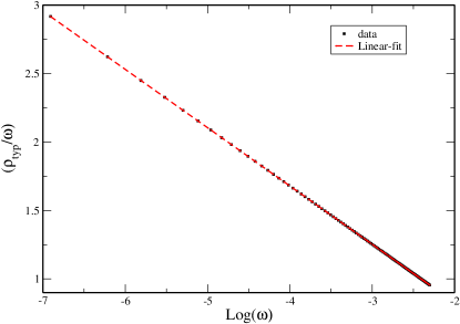
Figure 5: The behavior of TDOS for the pseudo gap model for $W=W_{c}1$, on semi-logarithmic scale, for small $0<\omega<0.1.$

Note, however, that if our result is examined only in a limited frequency interval, it can be represented as an power-law function, with an effective exponent $\beta(\omega)$, being a weak function of frequency.

To confirm this idea, we calculate $\beta(\omega)$ both using our analytical results, and also using the full numerical solution of the TMT equations. From our analytical solution, we can write

$$\rho_{c}(\omega)\approx a_{1}\omega(1-\frac{a_{2}}{a_{1}}\log\frac{\omega}{\omega_{0}})=a_{1}\omega^{\beta(\omega)},$$ (52)

where

$$\beta(\omega)=1+\log\frac{(1-\frac{a_{2}}{a_{1}}\log\omega+\frac{a_{2}}{a_{1}}\log\omega_{0})}{\log\omega}.$$ (53)

As we can see from Fig. 6, this analytical prediction is found to be in excellent quantitative comparison with the numerics. Within both methods, the effective exponent is $\beta(\omega)$ remains close to one in the entire critical region, therefore displaying moderate deviation from linear behavior found if the logarithmic corrections are ignored. We conclude that the mild logarithmic corrections we found near mobility edges can be neglected if we are not interested in the exact values for the critical exponents. These values generally cannot be expected to be accurately predicted by a mean-field approach such as TMT. This notion leads us to develop an effective (simplified) Landau theory for Anderson localization, which neglects such logarithmic corrections which preserving most qualitative trends found within TMT.

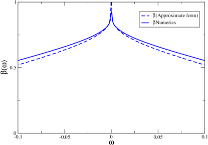
Figure 6: The behavior of effective exponent, at the critical disorder $W=W_{c1}.$

V Simplified Landau theory

In this section, we argue how the mean field solution of TMT equations can be simplified as we are not extremely close to the critical point, where mean-field theories such as TMT cannot be accurate in any case. Since we are interested in qualitative behavior of the order parameter and other physical observables across the phase diagram, and not only very close to the critical point, this approximation is justified and useful in predicting general trends. We have already seen that the only essential difference found within TMT, as compared to any mean-field theory is the emergence of mild logarithmic corrections to scaling. Ignoring them, therefore, provides us with a simplified formulation, where the equation of state, i.e. the self-consistency condition for the order parameter assumes simply a polynomial form, as any ordinary Landau theory. In the following, we formulate such a simplified Landau theory, and show that it captures the main qualitative trends, while preserving the key difference between the two classes of models of disorder we examine.

V.1 Analytical prediction of the effective Landau theory

As we have seen from Eq. (21), our TMT order-parameter satisfied a Landau-type equation of state, of polynomial form

$$r(\omega,W)+u_{1}(\omega)\varphi(\omega)+u_{2}(\omega)\varphi^{2}(\omega)+...=0.$$ (54)

To test these ideas, we use our numerical results for the TMT order parameter, and fit them to a polynomial form

$$\varphi(\omega)\sim\sqrt{r(\omega,W)}.$$ (55)

These results reproduce our previous results at half-filling ($\omega=0$), where $r(0,W)\sim(W_{c}-W)$, as well as the general trends for the approach to mobility edges elsewhere in the phase diagram.

V.2 Numerical fitting of the effective Landau coefficients for the pseudo-gap model

To test these ideas, we apply our effective Landau theory to the pseudo-gap model ($u_{1}=0$) close to the critical point. To do this, we note that according to Eq. (54), in this case to leading order

$$r(\omega,W)\sim\rho_{typ}^{2}(\omega,W),$$ (56)

and we can directly obtain the functional form of $r(\omega,W)$ from our numerical solution of the TMT equation. According to our Landau theory assumption, we expect it to be a smooth (analytic) function of frequency, and thus to assume a polynomial form

$$r(\omega,W)\sim B_{0}+B_{2}\omega^{2}-B_{4}\omega^{4}+\cdots$$ (57)

In the following, we calculate these coefficients numerically, as shown in Fig. 7 and Fig. 8. The coefficient $B_{0}$ vanishes linearly at the transition, consistent with previous results (See inset Fig. 4(a)). As it has been seen in Fig. 8, the coefficients $B_{2}$ and $B_{4}$ depend on $W$, but display on very weak dependence on the distance to the transition. As a final test, we show in Fig. 9 the behavior of TDOS, which is obtained both using our simplified version of TMT (simplified Landau theory) and the exact TMT solution. The numerical results indicate very similar behavior for order parameter within two different approaches. These results confirm the validity of our simplified Landau theory in capturing the main trends obtained form the exact solution of the TMT equations.

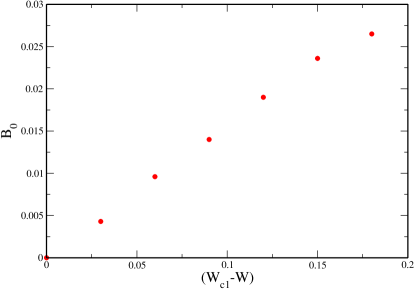
Figure 7: The behavior of the coefficient $B_{0}$ as a function of $(W_{c1}-W)$ close to the transition.

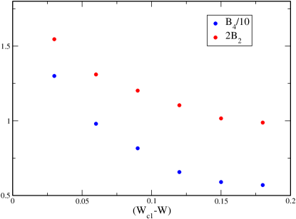
Figure 8: The Landau coefficient $2B_{2}$ and $\frac{B_{4}}{10}$ display only weak disorder dependence as the transition is approached.

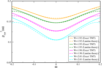
Figure 9: Comparison between the exact numerical TMT solution and the approximate solution, which is calculated within simplified Landau theory.

VI Conclusions

In summary, we carried out a detailed TMT study of the critical behavior for the Anderson metal-insulator transition, both analytically and numerically. Although the exact TMT theory gives us non-analytic critical behavior, we showed that the offending logarithmic corrections to scaling are not very significant if we are not too close to the transition. Given the fact that mean-field theories are generally not reliable very close to phase transitions, our results demonstrate that for practical purposes these subtle issues can safely be ignored, allowing us to formulate a much-simpler Landau-like formulation for Anderson localization. We also demonstrated that, within TMT, two different universality classes for the critical behavior may exist, depending on the qualitative form of disorder. We explored the opening of a soft pseudo-gap in the single-particle density of states near the Fermi energy, which is shown to emerge when the (renormalized) disorder is chosen to have a form appropriate for electrons interacting through long-range Coulomb interactions. In relevant cases, our results are found to be in excellent agreement with recent large-scale exact diagonalization resultsAmini et al. (2014), as well as with recent experimentsRichardella et al. (2010). Moreover, recently developed cluster refinements of TMT demonstratedEkuma et al. (2014a, b); Terletska et al. (2014) that significant corrections to (single site) TMT are only found very close to the Anderson transition. All these findings provide further evidence that TMT represents a flexible and practically useful tool for successfully describing the main qualitative trends for physical observables, in the vicinity of disorder-driven metal-insulator transitions.

Appendix A Expression for the cavity function for general band-structure models

For simplicity, we focus on the band center ($\omega=0$), where all quantities we self-consistently calculate (Green’s functions, cavity field, self-energies) are pure imaginary. In this case, there exists a simple relation between the typical Green’s function, the self energy, and the typical density of states, given by the expressions

$$G_{typ}=-\pi\rho_{typ},$$ (58)

and

$$\Sigma=-\Delta-\frac{1}{\pi\rho_{typ}}.$$ (59)

In order to close the self-consistent loop, we use Eq. (5), which contains the information on the form of the electronic band-structure, through the form of the "bare" (disorder-fee) density of states

$$G_{typ}(\omega)=\int d\omega^{\prime}\frac{\nu_{0}(\omega^{\prime})}{\omega-\omega^{\prime}-\Sigma}.$$ (60)

We expand the right-hand side of Eq.(60) in terms of $\frac{1}{\Sigma}$, which remains small as we approach to transition, and write

$$G_{typ}=-\frac{1}{\Sigma}-(\frac{1}{\Sigma})^{3}\int d\omega^{\prime}\omega^{\prime 2}\nu_{0}(\omega^{\prime})+\mathcal{O}(\frac{1}{\Sigma})^{5},$$ (61)

From Eq.(58) and Eq.(59), and keeping the leading terms in Eq.(61), we can obtain the general expression for cavity field as follows

$$\Delta=C\pi\rho_{typ}+\mathcal{O}(\rho_{typ}^{2}),$$ (62)

where

$$C=\int d\omega^{\prime}\omega^{\prime 2}\nu_{0}(\omega^{\prime}).$$ (63)

This result shows how the coefficient $C$ can be directly calculated at half-filling for any band-structure model. A similar a relation is valid even away from half-filling (as we also confirmed but detailed numerical work), but the specific numerical value depends on the relevant non-universal parameters. Therefore, as in other DMFT-like theories, to capture the qualitative aspect of the critical behavior, it is suffices to consider the simple semi-circular model density of states where $C=1$ for any filling and value of disorder.

References

- Dobrosavljević et al. (2012) V. Dobrosavljević, N. Trivedi, and J. M. Valles Jr, Conductor Insulator Quantum Phase Transitions (Oxford University Press, UK, 2012).
- Anderson (1958) P. Anderson, Physical Review 109, 1492 (1958).
- Mott (1990) N. F. Mott, Metal-Insulator Transition (Taylor & Francis, London, 1990).
- Georges et al. (1996) A. Georges, G. Kotliar, W. Krauth, and M. Rozenberg, Rev. Mod. Phys. 68, 13 (1996).
- Miranda and Dobrosavljevic (2005) E. Miranda and V. Dobrosavljevic, Reports on Progress in Physics 68, 2337 (2005).
- Dobrosavljević and Kotliar (1997) V. Dobrosavljević and G. Kotliar, Phys. Rev. Lett. 78, 3943 (1997).
- Miranda and Dobrosavljević (2001) E. Miranda and V. Dobrosavljević, Phys. Rev. Lett. 86, 264 (2001).
- Aguiar et al. (2003) M. C. O. Aguiar, E. Miranda, and V. Dobrosavljević, Phys. Rev. B 68, 125104 (2003).
- Song et al. (2008) Y. Song, R. Wortis, and W. Atkinson, Phys. Rev. B 77, 054202 (2008).
- Tran (2007) M.-T. Tran, Phys. Rev. B 76, 245122 (2007).
- Song et al. (2009) Y. Song, S. Bulut, R. Wortis, and W. A. Atkinson, Journal of Physics: Condensed Matter 21, 385601 (2009).
- Andrade et al. (2009) E. C. Andrade, E. Miranda, and V. Dobrosavljevic, Phys. Rev. Lett. 102, 206403 (2009).
- Semmler et al. (2010a) D. Semmler, J. Wernsdorfer, U. Bissbort, K. Byczuk, and W. Hofstetter, Phys. Rev. B 82, 235115 (2010a).
- Semmler et al. (2010b) D. Semmler, K. Byczuk, and W. Hofstetter, Phys. Rev. B 81, 115111 (2010b).
- Semmler et al. (2011) D. Semmler, K. Byczuk, and W. Hofstetter, Phys. Rev. B 84, 115113 (2011).
- Aguiar and Dobrosavljević (2013) M. C. O. Aguiar and V. Dobrosavljević, Phys. Rev. Lett. 110, 066401 (2013).
- Potthoff and Nolting (1999) M. Potthoff and W. Nolting, Phys. Rev. B 59, 2549 (1999).
- Helmes et al. (2008) R. Helmes, T. Costi, and A. Rosch, Phys. Rev. Lett. 101, 066802 (2008).
- Snoek et al. (2008) M. Snoek, I. Titvinidze, C. Toke, K. Byczuk, and W. Hofstetter, New Journal of Physics 10, 093008 (2008).
- Thouless et al. (1977) D. J. Thouless, P. W. Anderson, and R. G. Palmer, Philosophical Magazine 35, 137 (1977).
- M.Janssen (1998) M.Janssen, Phys. Rep. 295, 1 (1998).
- Dobrosavljević et al. (2003) V. Dobrosavljević, A. A. Pastor, and B. K. Nikolic, Europh. Lett. 62, 76 (2003).
- Byczuk et al. (2005) K. Byczuk, W. Hofstetter, and D. Vollhardt, Phys. Rev. Lett. 94, 056404 (2005).
- Aguiar et al. (2006) M. Aguiar, V. Dobrosavljević, E. Abrahams, and G. Kotliar, Phys. Rev. B 73, 115117 (2006).
- Byczuk et al. (2009) K. Byczuk, W. Hofstetter, and D. Vollhardt, Phys. Rev. Lett. 102, 146403 (2009).
- Aguiar et al. (2009) M. Aguiar, V. Dobrosavljević, E. Abrahams, and G. Kotliar, Phys. Rev. Lett. 102, 156402 (2009).
- Oliveira et al. (2014) W. S. Oliveira, M. C. O. Aguiar, and V. Dobrosavljević, Phys. Rev. B 89, 165138 (2014).
- Dobrosavljevic (2010) V. Dobrosavljevic, Int. J. Mod. Phys. B 24, 1680 (2010).
- Richardella et al. (2010) A. Richardella, P. Roushan, S. Mack, B. Zhou, D. Huse, D. Awschalom, and A. Yazdani, Science 327, 665 (2010).
- Efros and Shklovskii (1975) A. Efros and B. Shklovskii, Journal of Physics C: Solid State Physics 8, L49 (1975).
- Efros (1976) A. Efros, Journal of Physics C: Solid State Physics 9, 2021 (1976).
- Efros and Pollak (1985) A. L. Efros and M. Pollak, Electron-electron interactions in disordered systems (North Holland, 1985).
- Economou (2006) E. N. Economou, Greenś Functions in Quantum Physics (Springer, Berlin, 2006).
- Evers and Mirlin (2008) F. Evers and A. Mirlin, Reviews of Modern Physics 80, 1355 (2008).
- Massey and Lee (1996) J. Massey and M. Lee, Phys. Rev. Lett. 77, 3399 (1996).
- Pramudya et al. (2011) Y. Pramudya, H. Terletska, S. Pankov, E. Manousakis, and V. Dobrosavljević, Phys. Rev. B 84, 125120 (2011).
- Amini et al. (2014) M. Amini, V. E. Kravtsov, and M. Mller, New Journal of Physics 16, 015022 (2014).
- Polyanin and Manzhirov (2008) A. D. Polyanin and A. V. Manzhirov, Handbook of integral equations (Chapman and Hall/CRC, 2008).
- Ekuma et al. (2014a) C. E. Ekuma, H. Terletska, Z. Y. Meng, J. Moreno, M. Jarrell, S. Mahmoudian, and V. Dobrosavljevic, Journal of Physics: Condensed Matter 26, 274209 (2014a).
- Ekuma et al. (2014b) C. E. Ekuma, H. Terletska, K.-M. Tam, Z.-Y. Meng, J. Moreno, and M. Jarrell, Phys. Rev. B 89, 081107 (2014b).
- Terletska et al. (2014) H. Terletska, C. E. Ekuma, C. Moore, K.-M. Tam, J. Moreno, and M. Jarrell, Phys. Rev. B 90, 094208 (2014).