Shaping coherent excitation of atoms and molecules
by a train of ultrashort laser pulses

Abstract

We propose a mechanism to produce a superposition of atomic and molecular states by a train of ultrashort laser pulses combined with weak control fields. By adjusting the repetition rate of the pump pulses and the intensity of the coupling laser, one can suppress a transition, while simultaneously enhancing the desired transitions. As an example various superpositions of states of the $K_{2}$ molecule are shown.

I INTRODUCTION

Population transfer to a desired coherent superposition of atomic and molecular states (i.e. a wavepacket) has been a major goal during the last three decades and continues to be a challenge for instance for implementation of chemical and biological processes rice ; rabitz ; wenach , for fast quantum information processing lukin ; saffman ; jakch ; tesch and for nonlinear optics Jain .

Besides extensions of $\pi$-pulse techniques Allen ; Shore ; Holthaus ; lifting and of brute-force optimal control Glaser , mechanisms to produce superpositions of two states in atoms based on adiabatic passage (in nanosecond regime) have been proposed Yatsenko ; lifting ; Sangouard and demonstrated Rickes ; Sautenkov ; Oberst . Extending such techniques to an ultrafast regime and for molecular systems is of particular interest. Another ultrafast spectroscopic technique is Impulsive Stimulated Raman Scattering (ISRS) that provides vibrational structural information with high temporal and spectral resolution Yan ; Nazarkin ; Wittmann . ISRS excitation of coherent phonons, molecular vibrations, and other excitations (including rotational, electronic, and spin) plays important roles in femtosecond pulse interactions with molecules, crystals, glasses (including optical fibers), semiconductors, and metals Yan . This is an effective approach to determine the dynamics of vibrational molecular motion Bartels .

Recent progress has allowed the development of mode-locked laser systems producing mutually phase-coherent ultrashort laser pulses of high intensity with arbitrary controllable amplitudes, of stable frequency and of adjustable delay time (see for instance Hansch ; Ye ). Theoretical Vitanov ; FelintoOC2003 ; Jakubetz and experimental FelintoExp ; YeScience analysis in a few level systems have shown that a resonant $\pi$-pulse (or generalized $\pi$-pulse Holthaus ; lifting ) can be split into trains of fractional $\pi$-pulses and can lead to the accumulation of population in a target state for appropriate delays. The main point is that weak pulses can then be used preventing detrimental destructive effects such as ionization. For more complicated systems, populating some chosen states among a set of levels all within the broad ultrashort pulse spectrum is a major issue. However one can exploit one of the main properties of the associated frequency comb, that is its extremely small resolution, given by the width of the comb s teeth in the frequency domain, much better than the one determined by the Fourier transform of a single pulse in the train. High degree of population transfer to a single vibrational state of an electronic excited state has been indeed numerically shown by a train of fs laser pulses by choosing the pulse repetition period as noninteger multiple of the vibrational period araujo . Recently a so-called piecewise adiabatic passage method, based on the combination of adiabatic passage, trains of pulses, and pulse-shaping techniques, has been proposed shapiro ; shapiro2 .

In this paper, we propose an alternate robust and efficient method for population transfer to a desired superposition in multilevel systems using a train of pulses combined with weak controlled lasers. We derive analytical formulas in the impulsive and perturbative regimes for the ultrashort pump pulses.

We consider a system of level configuration shown in Fig. 1 interacting with a train of ultrashort femtosecond laser pulses, whose spectrum is wide enough to overlap all the upper states, while a narrow-band weak laser couples, for example, the upper level 1 with an auxiliary state 4. We consider three upper levels for simplicity, but the proposed mechanism can be directly extended to any number of upper-lying levels. By adjusting the repetition rate of the pump pulses with respect to the Rabi frequency $\Omega_{c}$ of the coupling field, this scheme enables one to cancel out the strong transition $0\rightarrow 1$ from the pump field, while enhancing the transitions $0\rightarrow i,i=2,3$. To give an insight into the proposed mechanism, let us consider the interaction of the system with two consecutive identical pump pulses in resonance on the transition $0\rightarrow 1$, with a time delay $\tau_{d}$, which is larger as compared to the pulse duration $T$. In the low intensity regime, the atomic state amplitudes $C_{1,2,3}$ after the first pump pulse are: $C_{j}\sim\theta_{j}=\int\Omega_{j}(t)e^{i\Delta_{j}}dt\ll 1,\;j=1,2,3$, with $\Omega_{j}$ the pump Rabi frequencies corresponding to the respective $0\rightarrow j$ transitions [see Eqs. (2) and (3) for the definition of the fields and the Rabi in this paper]. At the end of the second pulse they take the forms: $C_{1}\sim\theta_{1}+\theta_{1}\cos(\Omega_{c}\tau_{d})$ and $C_{2,3}\sim 2\theta_{2}$ showing that when the delay time $\tau_{d}$ is such that

$$\Omega_{c}\tau_{d}=\pi(1+2k),$$ (1)

with $k$ an integer, the population on the level 1 vanishes, while it increases four times on states 2 and 3: The excitation amplitudes of the two pump pulses add coherently for an appropriate delay Vitanov . Hereafter we assume that the upper-lying levels are harmonic, such that the condition $\omega_{ij}\tau_{d}=2\pi k_{ij}$ applies, with $k_{ij}$ an integer and $\omega_{ij}=\omega_{j}-\omega_{i}$ the frequency splitting between the upper levels of energies $\omega_{j}$. This condition is essential to accumulate population in the upper states from pulse to pulse. Therefore, as long as the pulse delay $\tau_{d}$ remains well smaller than the atomic decoherence time, the second pulse allows the selective excitation of a superposition of states 2 and 3. Our method does not suffer from a high sensitivity to laser-field instabilities. We show below that the efficiency of the process is preserved even when the condition (1) is not well satisfied.

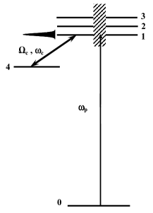
Figure 1: Level scheme illustrating the excitation of three upper states by the ultrashort pump laser. A cw coupling field drives the auxiliary transition $1\rightarrow 4.$

The paper is organized as follows. In the next section we derive and solve the basic equations for the time evolution of the state amplitudes in the impulsive and perturbative regimes. In Sec. III we apply the proposed technique to produce superpositions of states in an electronic state of the molecule $K_{2}$. Our conclusions are summarized in Sec. IV.

II Mechanism of selective excitation

II.1 The model

In our scheme (Fig. 1), the upper states 1, 2 and 3 are populated via a single photon excitation by a train of $m$ identical and non-overlapping ultrashort laser pulses, whose spectrum is centered on the resonance with the transition $0\rightarrow 1$ and is wide enough that upon interacting with each pulse, all the states 1, 2 and 3 are excited simultaneously: $T^{-1}\sim\Gamma>\omega_{31}$. Here $\Gamma$ is the spectral width of the laser fields and $\omega_{31}$ is the frequency splitting of the levels 1 and 3. We assume that the narrow-band coupling field is in exact resonance with the transition $1\rightarrow 4$ with the pulse duration much longer than that of the pump pulses $T$. In what follows, we neglect the Doppler broadening because it is small as compared to $\Gamma$.

The pump $E_{p}(t)$ and coupling $E_{c}(t)$ field amplitudes of respective carrier frequencies $\omega_{p}$ and $\omega_{c}$ are of the form (in complex notation)

$$E_{p}(t)=\sum_{i=1}^{m}\mathcal{E}_{i}(t)e^{i\omega_{p}t},\quad E_{c}(t)=\mathcal{E}_{c}(t)e^{i\omega_{c}t},$$ (2)

with the same shape $f(t)$ for all $m$ pump pulses that determines the time dependence of $\mathcal{E}_{i}(t)=\mathcal{E}_{0}f(t-t_{1}-(i-1)\tau_{d})$, and the delay $\tau_{d}$ between two consecutive pulses. The interaction of the system with the pump and coupling fields is determined by their Rabi frequencies at the corresponding transitions

$$\Omega_{p}^{(j)}(t)=\frac{\mu_{j}}{\hbar}\mathcal{E}_{i}(t),\quad\Omega_{c}(t)=\frac{\mu_{14}}{\hbar}\mathcal{E}_{c}(t),$$ (3)

where $\mu_{ij}$ is the dipole matrix element of the transition $i\rightarrow j=1,2,3$ and the notation $\mu_{j}\equiv\mu_{0j}$. We consider for simplicity a time independent coupling field. Our results generalize for a pulsed coupling field of much longer duration than the pump field. In the rotating wave approximation with respect to the pump field, the Hamiltonian of the system is given by

$$H=-\hbar\sum_{j=1}^{3}\bigl{(}\Omega_{p}^{(j)}\sigma_{j0}-\Delta_{j}\sigma_{jj}\bigr{)}-\hbar\Delta_{1}\sigma_{44}-\hbar\Omega_{c}\sigma_{41}+h.c.,$$ (4)

where $\sigma_{ij}=|i\rangle\langle j|$ are the atomic operators and $\Delta_{j}=\omega_{j0}-\omega_{p}$ is two-photon detuning of the pump field from the $0\rightarrow j,\ j=1,2,3$ transition. The state $|\psi(t)\rangle=\sum_{i}C_{i}(t)|{i}\rangle$ of the atom satisfies the Schrödinger equation $\dot{C_{i}}(t)=-\frac{i}{\hbar}\sum_{k}\langle i|H|k\rangle C_{k}(t),$ which leads to the equations for the atomic state amplitudes

$$\dot{C}_{0}(t) = i\sum_{j=1,2}\Omega_{p}^{(j)\ast}C_{j}(t),$$ (5a)

$$\dot{C}_{1}(t) = -i\Delta_{1}C_{1}+i\Omega_{p}^{(1)}C_{0}(t)+i\Omega_{c}C_{4},$$ (5b)

$$\dot{C}_{2,3}(t) = -i\Delta_{2,3}C_{2,3}+i\Omega_{p}^{(2,3)}C_{0}(t),$$ (5c)

$$\dot{C}_{4}(t) = -i\Delta_{1}C_{4}+i\Omega_{c}^{\ast}C_{1}$$ (5d)

with the initial conditions

$$C_{0}(-\infty)=1,\quad C_{j\neq 0}(-\infty)=0.$$ (6)

II.2 Solution in the impulsive regime

In the general case, Eqs. (5) do not provide an analytic solution. However, in the regime of low intensity of the coupling field with respect to the pump fields: $\Omega_{c}\ll\Omega_{p}$ and in the impulsive (or sudden) approximation for the ultrashort pump pulse by disregarding the detunings $\Delta_{j}T\ll 1$ UTDST , one can determine the solution (see Appendix). Equations (19) show the dependence of the state amplitudes after the $(n+1)$-st pulse depending on the amplitudes after the $n$-th pulse ($n=1,2,...$). For the sequence of two pump pulses right after the interaction with the second pump pulse, Eqs. (19) lead to

$$C_{0}(t_{2}^{+}) = \cos^{2}\theta-\frac{1}{\mu^{2}}\bigl{(}\mu_{1}^{2}e^{-i\Delta_{1}\tau_{d}}\cos(\Omega_{c}\tau_{d})+\mu_{2}^{2}e^{-i\Delta_{2}\tau_{d}}+\mu_{3}^{2}e^{-i\Delta_{3}\tau_{d}}\bigr{)}\sin^{2}\theta$$ (7a)

$$C_{1}(t_{2}^{+}) = i\frac{\mu_{1}}{2\mu}\sin 2\theta\Bigl{[}1+\frac{1}{\mu^{2}}\Bigl{(}\mu_{1}^{2}e^{-i\Delta_{1}\tau_{d}}\cos(\Omega_{c}\tau_{d})+\sum_{k=2}^{3}\mu_{k}^{2}e^{-i\Delta_{k}\tau_{d}}\Bigr{)}\Bigr{]}$$ (7b)

$$+i\frac{\mu_{1}}{\mu^{3}}\sin\theta\Bigl{[}\Bigl{(}\sum_{k=2}^{3}\mu_{k}^{2}\Bigr{)}e^{-i\Delta_{1}\tau_{d}}\cos(\Omega_{c}\tau_{d})-\Bigl{(}\sum_{k=2}^{3}\mu_{k}^{2}e^{-i\Delta_{k}\tau_{d}}\Bigr{)}\Bigr{]}$$

$$C_{2}(t_{2}^{+}) = i\frac{\mu_{2}}{2\mu}\sin 2\theta\Bigl{[}1+\frac{1}{\mu^{2}}\Bigl{(}\mu_{1}^{2}e^{-i\Delta_{1}\tau_{d}}\cos(\Omega_{c}\tau_{d})+\sum_{k=2}^{3}\mu_{k}^{2}e^{-i\Delta_{k}\tau_{d}}\Bigr{)}\Bigr{]}$$ (7c)

$$+i\frac{\mu_{2}}{\mu^{3}}\sin\theta\Bigr{\{}\mu_{1}^{2}\Bigl{[}e^{-i\Delta_{2}\tau_{d}}-e^{-i\Delta_{1}\tau_{d}}\cos(\Omega_{c}\tau_{d})\Bigr{]}+\mu_{3}^{2}\bigl{(}e^{-i\Delta_{2}\tau_{d}}-e^{-i\Delta_{3}\tau_{d}}\bigr{)}\Bigr{\}}$$

$$C_{3}(t_{2}^{+}) = C_{2\leftrightarrow 3}(t_{2}^{+}),$$ (7d)

$$C_{4}(t_{2}^{+}) = -\frac{\mu_{1}}{\mu}e^{-i\Delta_{1}\tau_{d}}\sin\theta\sin(\Omega_{c}\tau_{d})$$ (7e)

with

$$\theta=\frac{\mu}{\hbar}\int\mathcal{E}(t)dt,\quad\mu=\biggl{(}\sum_{k=1}^{3}\mu_{k}^{2}\biggr{)}^{1/2},$$ (8)

and $\int\mathcal{E}(t)dt$ the area of each pump pulse (considered invariant from pulse to pulse). When the upper-lying states 1,2,3 are harmonic such that (i) $\omega_{ij}\tau_{d}=2\pi n$, (ii) condition (1) is fulfilled, and (iii) the pump pulses are resonant with one of any transitions $0\rightarrow i$, i.e. $\Delta_{i}=0$, and implying $\Delta_{j}\tau_{d}=2\pi n_{j}$ for all $j$ (with $n_{j}$ an integer) from condition (i), these equations take the simpler form

$$C_{0}(t_{2}^{+}) = \cos^{2}\theta-\frac{\mu_{2}^{2}+\mu_{3}^{2}-\mu_{1}^{2}}{\mu^{2}}\sin^{2}\theta,$$ (9a)

$$C_{1}(t_{2}^{+}) = 2i\frac{\mu_{1}}{\mu}\frac{\mu_{2}^{2}+\mu_{3}^{2}}{\mu^{2}}\sin\theta(\cos\theta-1),$$ (9b)

$$C_{2}(t_{2}^{+}) = i\frac{\mu_{2}}{\mu}\bigl{(}\frac{\mu_{2}^{2}+\mu_{3}^{2}}{\mu^{2}}\sin 2\theta+\frac{2\mu_{1}^{2}}{\mu^{2}}\sin\theta\bigr{)},$$ (9c)

$$C_{3}(t_{2}^{+}) = C_{2},(2\leftrightarrow 3),C_{4}(t_{2}^{+})=0.$$ (9d)

This shows that, in order to cancel out the population transfer to state 1 while increasing the population of states 2 and 3, only the limit of weak pump excitation ($\theta\ll 1$) is suitable since it leads to $\cos\theta-1=O(\theta^{2})$.

II.3 Solution in the perturbative regime

If we consider that each pump pulse is weak: $\Omega_{j}T\ll 1$, we can perturbatively calculate the solution of Eqs. (5) (without invoking explicitly the shortness of the pump pulse). We obtain with correction of order $O(\theta^{2})$:

$$C_{1}(t_{n+1}^{+}) = i\theta_{1}+e^{-i\Delta_{1}\tau_{d}}\Bigl{[}C_{1}(t_{n}^{+})\cos(\Omega_{c}\tau_{d})$$ (10a)

$$+iC_{4}(t_{n}^{+})\sin(\Omega_{c}\tau_{d})\Bigr{]},$$

$$C_{j}(t_{n+1}^{+}) = i\theta_{j}+e^{-i\Delta_{j}\tau_{d}}C_{j}(t_{n}^{+}),\quad j=2,3$$ (10b)

$$C_{4}(t_{n+1}^{+}) = e^{-i\Delta_{1}\tau_{d}}\bigl{[}iC_{1}(t_{n}^{+})\sin(\Omega_{c}\tau_{d})$$ (10c)

$$+C_{4}(t_{n}^{+})\cos(\Omega_{c}\tau_{d})\bigr{]}$$

with

$$\theta_{j}=\frac{\mu_{j}}{\hbar}\int{\cal E}(t)e^{i\Delta_{j}t}dt$$ (11)

the Fourier spectral component of the Rabi frequency of the pump pulse at frequency $\Delta_{j}$. We remark that we recover these equations (10) from Eqs. (19) using $\sin\theta=\theta+O(\theta^{3})$ and $\cos\theta=1+O(\theta^{2})$ except for the phase in the $\theta_{j}$’s that are neglected in the impulsive regime.

II.3.1 Selective excitation to a single state araujo

To excite a single state, say state 1, no control field is required : $\Omega_{c}=0$, and the pump needs to be resonant with the target state: $\Delta_{1}=0$. In that case one can determine the coefficients after $n$ pulses from Eqs. (10):

$$C_{1}(t_{n}^{+}) = in\theta_{1},$$ (12a)

$$C_{j=2,3}(t_{n}^{+}) = ie^{-i(n-1)\Delta_{j}\tau_{d}/2}\frac{\sin(\frac{n}{2}\Delta_{j}\tau_{d})}{\sin(\frac{1}{2}\Delta_{j}\tau_{d})}\theta_{j}.\qquad$$ (12b)

This shows that population in the target state accumulates linearly as a function of the number of the ultrashort pulses. Population does not coherently accumulate for large $n$ in the other state if one chooses $\Delta_{j}\tau_{d}$ well different from $2\pi k$, $k$ an integer. This effect is optimal when

$$\Delta_{j}\tau_{d}=\pi(1+2k).$$ (13)

The population transfer to state 1 is closer to 1 when the total area of the pump pulses is 2$\pi$. (This value obtained here 2$\pi$ is due to the definition of the fields (2) and the Rabi frequencies (3); This corresponds to a “$\pi$-pulse” transfer of a single strong field.) The resulting selective excitation is thus very robust with respect to $\Delta_{j}\tau_{d}$.

II.3.2 Selective excitation to a superposition of states

To excite a superposition of states, one has to impose

$$\Delta_{j}\tau_{d}=2\pi k_{j}$$ (14)

with $k_{j}$ an integer, which leads to

$$C_{j=2,3}(t_{n}^{+})=ie^{-i(n-1)\pi}n\theta_{j}.$$ (15)

This condition can be satisfied when the upper-lying states within the bandwidth of a single pulse are harmonic.

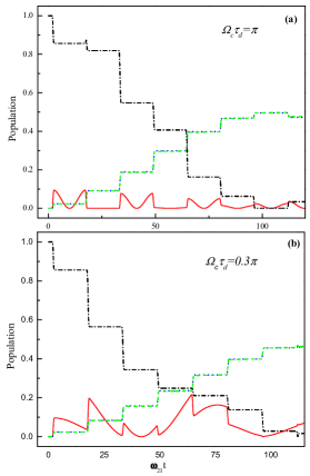
Figure 2: (color online)Populations of atomic ground state (dash-dotted, black) and upper levels 1 (solid, red), 2 (dotted, blue) and 3 (dashed, green) excited by a train of the pump pulses for $\mu_{2}=\mu_{3}=0.5\mu_{1},T=0.3\omega_{21}$ and a) $\Omega_{c}\tau_{d}=\pi$; b) $\Omega_{c}\tau_{d}=0.3\pi$.

We now show that the control field allows to remove the transition to the state to which this control field is resonantly coupled. We choose state 1 to have this feature, i.e. $\Delta_{1}=0$. From Eqs. (10), we get after $n$ pulses:

$$C_{1}(t_{n}^{+}) = i\cos\Bigl{(}\frac{n-1}{2}\Omega_{c}\tau_{d}\Bigr{)}\frac{\sin(\frac{n}{2}\Omega_{c}\tau_{d})}{\sin(\frac{1}{2}\Omega_{c}\tau_{d})}\theta_{1},$$ (16a)

$$C_{4}(t_{n}^{+}) = i\sin\Bigl{(}\frac{n-1}{2}\Omega_{c}\tau_{d}\Bigr{)}\frac{\sin(\frac{n}{2}\Omega_{c}\tau_{d})}{\sin(\frac{1}{2}\Omega_{c}\tau_{d})}\theta_{1}.\qquad$$ (16b)

The populations do not accumulate in states 1 and 4 if one chooses $\Omega_{c}\tau_{d}$ well different from $2\pi k$, $k$ an integer. This effect is optimal when $\Omega_{c}\tau_{d}=\pi(1+2k)$ [see condition (1)]. The value for $k=0$ corresponds to a $\pi$ area, i.e. a “$\pi/2$-pulse”, for the control field in this model. We remark that such a cancelation of the transfer to state 1 is thus expected to be robust with respect to a precise area of the control field.

Thus, by choosing the number of the pump-pulses, one can achieve the coherent selective superposition of the levels 2 and 3, while keeping the state 1 almost empty.

In Fig. 2a we show the results of numerical integration of Eqs. (5) obtained under the conditions mentioned above using Gaussian shape $f(t)=\exp(-t^{2}/T^{2})$ for the pump pulses. Very similar results are obtained, when the condition (1) is significantly violated, as shown in Fig. 2b. This demonstrates the robustness of our scheme with respect to the coupling field instabilities as predicted above.

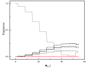
Figure 3: (color online) Populations of $K_{2}$ of the ground state $v^{\prime\prime}=0$ (dotted, black), the upper state $v^{\prime}=10$ (solid, red) and the other states $v^{\prime}=8,9,11,12,13$ (dashed lines).

We apply the proposed mechanism in the next section to produce a selective coherent superposition of vibrational states in a molecular electronic state.

III Application to the potassium dimer

We consider the excitation of the potassium dimer $K_{2}$ lyyra . The molecule is supposed to be prepared in the ground vibrational state $v^{\prime\prime}=0$ of the electronic state $X^{1}\Sigma_{g}^{+}$. The excited state is chosen to be the first excited electronic state $A^{1}\Sigma_{u}^{+}$ (of lifetime 28ns). For simplicity in the calculations the dependence of the electric dipole moment on internuclear distance is ignored. The pump pulses are assumed to be transform limited of Gaussian envelope $f(t)=\exp(-t^{2}/T^{2})$ with duration $T=150$fs and peak intensity $I_{p}^{\max}\sim 10^{11}$ W/cm². We assume the pump pulses to be on resonance with the transition $v^{\prime\prime}=0\rightarrow v^{\prime}=10$ ($\omega_{L}\simeq 11800cm^{-1}$). The excited vibrational levels $v^{\prime}=8,9,...,13$ are within the spectrum of the pump field and are expected to be populated. Our main goal is to suppress the strongest transition $v^{\prime}=10$ of the upper vibrational levels.

Figure 4: Histogram of the vibrational population distribution after excitation without (upper frame) and with (lower frame) the coupling field.

Figure 5: Histogram of the vibrational population distribution after excitation by the same pulses used in Fig. 4 but of duration 600 fs.

Figure 6: Histogram of the vibrational population distribution when the states $v^{\prime}=8,10,12,13$ are coupled to auxiliary states by coupling fields.

We solve numerically equations for atomic population amplitudes similar to Eq. (5), including all the relevant vibrational states of the problem, using the above parameters, and with the requirement that the conditions (1) and $\omega_{9^{\prime}10^{\prime}}=2\pi k\tau_{d}$ are fulfilled, where $\omega_{9^{\prime}10^{\prime}}$ is the frequency splitting of the vibrational states $v^{\prime}=9$ and $v^{\prime}=10$ of the upper electronic state. For $\omega_{9^{\prime}10^{\prime}}=67.3\text{cm}^{-1}$ the delay time between the subpulses is $\tau_{d}\simeq 3\text{ps}$. Note, that frequency splitting of the upper lying levels is almost equidistant. The coupling field couples the state $v^{\prime}=10$, of largest dipole moment element among the states within the bandwidth of a single pump, with an auxiliary electronic state of the potassium dimer, e.g. $b^{3}\Pi_{u}$. Figure 3 shows the dynamics of the populations of the vibrational levels, when it is excited by a train of identical pulses. To calculate the populations we have used the Franck-Condon factors and the corresponding eigenfrequencies, which are well known for vibrational levels of $K_{2}$ molecules lyyra . The chosen values of the parameters: $\Omega_{c}\simeq 0.2\omega_{9^{\prime}10^{\prime}}\ll\Omega_{p}^{max}\simeq 0.6\omega_{9^{\prime}10^{\prime}}$ and $\theta^{2}(\infty)\sim 0.15$ provide all the necessary conditions for the analytical analysis made in the previous section to be valid. As it is seen in Fig. 3, after the interaction of the molecule with 8 pulses, all the population is distributed between the upper vibrational levels $v^{\prime}=8,9,11,12,13$ (dotted lines), while the level $v^{\prime}=10$ (red, solid line) stays almost unpopulated. To have a more complete picture of the process, Fig. 4 displays the histogram of the population distribution in the upper-lying states. In the absence of the coupling field the population is distributed between all upper vibrational states (Fig. 4 upper frame). But if the coupling field is on (Fig. 4 lower frame), the strongest transition is dramatically suppressed. Adapting the duration of the pulses allows one to modify the shape of the superposition, reducing the population of the upper states, as it is shown in Fig. 5. Here the duration of the pump pulses are taken to be four times larger than that of the cases considered previously. To suppress some components of the superposition one can apply other fields coupled to the undesired states from different auxiliary states. As an example in Fig. 6 the levels $v^{\prime}=8,10,12,13$ are coupled with other molecular states which leads to a coherent superposition of only two states $v^{\prime}=9,11$. Thus, we have shown that the coupling fields allow the decreasing of the populations of the undesired states and the enhancement of the populations of the other states well within the bandwidth of a single pump.

IV Conclusion

In this paper we have proposed a robust and simple mechanism for the coherent excitation of the molecule or atom to a superposition of pre-selected states by a train of fs laser pulses, combined with narrow-band weak laser fields coupling the undesired states well within the bandwidth of a single pulse to auxiliary states. The coupling fields allow the cancelation of specific transitions from the ground state to a set of states $i$ when they induce a coherence between each state $i$ and an auxiliary state (all different). We remark that these predictions of selective coherent excitation could be measured experimentally by a sensitive method such as the one developed in gogyan .

Acknowledgments

This research has been conducted in the scope of the International Association Laboratory IRMAS. We also acknowledge the support from the Armenian Science Ministry (Grant No 096), the French Agence Nationale de la Recherche (Project CoMoC) and the Marie Curie Initial Training Network Grant No. CA-ITN-214962-FASTQUAST.

*

Appendix A General solution in the impulsive regime

We integrate Eqs. (5) over the time of interaction with the n${}^{\text{th}}$ pump pulse in the impulsive approximation, disregarding the detunings $\Delta_{j}T\ll 1$ and where to a good approximation the weak $\Omega_{c}$ - terms can be neglected. This yields a simple solution right after the n${}^{\text{th}}$ pump pulse at time $t=t_{n}^{+}$ (considered interacting at $t=t_{n}$), from the solution right before the pulse at time $t=t_{n}^{-}$:

$$C_{0}(t_{n}^{+}) = C_{0}(t_{n}^{-})\cos\theta+i\bar{C}_{n}^{-}\sin\theta$$ (17a)

$$C_{j}(t_{n}^{+}) = C_{j}(t_{n}^{-})+i\frac{\mu_{j}}{\mu}C_{0}(t_{n}^{-})\sin\theta$$

$$+ \frac{\mu_{j}}{\mu}\bar{C}_{n}^{-}(\cos\theta-1),\quad j=1,2,3$$ (17b)

$$C_{4}(t_{n}^{+}) = C_{4}(t_{n}^{-}),$$ (17c)

where $\mu=\sqrt{\sum_{k=1}^{3}\mu_{k}^{2}}$, $\theta=\frac{\mu}{\hbar}\int\mathcal{E}(t)dt$ with $\int\mathcal{E}(t)dt$ the area of each pump pulse (considered invariant from pulse to pulse), and $\bar{C}_{n}^{-}=[\sum_{k=1}^{3}\mu_{k}C_{k}(t_{n}^{-})]/\mu$. After the n${}^{\text{th}}$ pulse turned off, the amplitudes $C_{0}$, $C_{2}$ and $C_{3}$ evolve freely up to $t\sim t_{n}+\tau_{d}$, $\tau_{d}\gg T$:

$$C_{0}(t) = C_{0}(t_{n}^{+}),$$ (18a)

$$C_{j}(t) = e^{-i\Delta_{j}(t-t_{n})}C_{j}(t_{n}^{+}),\ j=2,3,$$ (18b)

while $$C_{1}(t) C_{4}(t) t_{n+1}>t>t_{n}$$ and , are found from Eqs. (5) with the initial values (17-17c) as

$$C_{1}(t) = e^{-i\Delta_{1}(t-t_{n})}\Bigl{\{}C_{1}(t_{n}^{+})\cos\bigl{[}\Omega_{c}(t-t_{n})\bigr{]}$$ (18c)

$$+iC_{4}(t_{n}^{+})\sin\bigl{[}\Omega_{c}(t-t_{n})\bigr{]}\Bigr{\}},$$

$$C_{4}(t) = e^{-i\Delta_{1}(t-t_{n})}\Bigl{\{}iC_{1}(t_{n}^{+})\sin\bigl{[}\Omega_{c}(t-t_{n})\bigr{]}$$ (18d)

$$+C_{4}(t_{n}^{+})\cos\bigl{[}\Omega_{c}(t-t_{n})\bigr{]}\Bigr{\}},$$

We iterate the above procedure for all the ultrashort pump pulses:

$$C_{0}(t_{n+1}^{+}) = C_{0}(t_{n}^{+})\cos\theta+\frac{i}{\mu}\sin\theta\Bigl{\{}\mu_{1}e^{-i\Delta_{1}\tau_{d}}\Bigl{[}C_{1}(t_{n}^{+})\cos(\Omega_{c}\tau_{d})+iC_{4}(t_{n}^{+})\sin(\Omega_{c}\tau_{d})\Bigr{]}+\sum_{k=2}^{3}\mu_{k}e^{-i\Delta_{k}\tau_{d}}C_{k}(t_{n}^{+})\Bigr{\}},\qquad\ \$$ (19a)

$$C_{1}(t_{n+1}^{+}) = i\frac{\mu_{1}}{\mu}C_{0}(t_{n}^{+})\sin\theta+e^{-i\Delta_{1}\tau_{d}}\Bigl{[}C_{1}(t_{n}^{+})\cos(\Omega_{c}\tau_{d})+iC_{4}(t_{n}^{+})\sin(\Omega_{c}\tau_{d})\Bigr{]}\Bigl{[}1+\frac{\mu_{1}^{2}}{\mu^{2}}(\cos\theta-1)\Bigr{]}$$ (19b)

$$+\frac{\mu_{1}}{\mu}(\cos\theta-1)\sum_{k=2}^{3}\frac{\mu_{k}}{\mu}e^{-i\Delta_{k}\tau_{d}}C_{k}(t_{n}^{+}),$$

$$C_{2}(t_{n+1}^{+}) = i\frac{\mu_{2}}{\mu}C_{0}(t_{n}^{+})\sin\theta+e^{-i\Delta_{2}\tau_{d}}C_{2}(t_{n}^{+})\Bigl{[}1+\frac{\mu_{2}^{2}}{\mu^{2}}(\cos\theta-1)\Bigr{]}$$ (19c)

$$+\frac{\mu_{2}}{\mu}(\cos\theta-1)\Bigl{\{}\frac{\mu_{1}}{\mu}e^{-i\Delta_{1}\tau_{d}}\Bigl{[}C_{1}(t_{n}^{+})\cos(\Omega_{c}\tau_{d})+iC_{4}(t_{n}^{+})\sin(\Omega_{c}\tau_{d})\Bigr{]}+\frac{\mu_{3}}{\mu}e^{-i\Delta_{3}\tau_{d}}C_{3}(t_{n}^{+})\Bigr{\}},$$

$$C_{3}(t_{n+1}^{+}) = C_{2\leftrightarrow 3}(t_{n+1}^{+}),$$ (19d)

$$C_{4}(t_{n+1}^{+}) = e^{-i\Delta_{1}\tau_{d}}\bigl{[}iC_{1}(t_{n}^{+})\sin(\Omega_{c}\tau_{d})+C_{4}(t_{n}^{+})\cos(\Omega_{c}\tau_{d})\bigr{]}.$$ (19e)

Eq. (19d) means that the amplitude $C_{3}$ has the same expression as $C_{2}$ (19c) but exchanging the indices 2 and 3.

References

• (1) H. Rabitz, R. de Vivie-Riedle, M. Motzkus, and K. L. Kompa, Science 288, 824 (2000).
• (2) S. A. Rice and M. Zhao, Optical Control of Molecular Dynamics (Wiley, New York, 2000).
• (3) T. C. Weinacht, J. Ahn, and P. H. Bucksbaum, Nature (London) 397, 233 (1999).
• (4) M. D. Lukin, M. Fleischhauer, R. Cote, L. M. Duan, D. Jaksch, J. I. Cirac, and P. Zoller, Phys. Rev. Lett. 87,037901 (2001).
• (5) M. Saffman and T. G. Walker, Phys. Rev. A 66, 065403 (2002).
• (6) D. Jaksch, J. I. Cirac, P. Zoller, S. L. Rolston, R. Cote, and M. D. Lukin, Phys. Rev. Lett. 85, 2208 (2000).
• (7) C. M. Tesch and R. de Vivie-Riedle, Phys. Rev. Lett. 89, 157901 (2002).
• (8) M. Jain, H. Xia, G.Y. Yin, A.J. Merriam, and S.E. Harris, Phys. Rev. Lett. 77, 4326 (1996).
• (9) J. Allen and J.H. Eberly, Optical resonance and two-level atoms (Wiley, New York, 1975).
• (10) B.W. Shore, The Theory of Coherent Atomic Excitation, Wiley, New York, 1990.
• (11) M. Holthaus and B. Just, Phys. Rev. A 49, 1950 (1994).
• (12) L. P. Yatsenko, S. Guérin, and H. R. Jauslin, Phys. Rev. A 70, 043402 (2004).
• (13) T.E. Skinner, T.O. Reiss, B. Luy, N. Khaneja, and S. Glaser, J. Magn. Reson. 167, 68 (2004).
• (14) L.P. Yatsenko, N.V. Vitanov, B.W. Shore, T. Rickes, and K. Bergmann, Opt. Commun. 204, 413 (2002).
• (15) N. Sangouard, S. Guérin, L.P. Yatsenko, and T. Halfmann, Phys. Rev. A 70, 013415 (2004).
• (16) T. Rickes, J.P. Marangos and T. Halfmann, Opt. Commun. 227, 133 (2003).
• (17) V.A. Sautenkov, C.Y. Ye, Y.V. Rostovtsev, G.R. Welch, and M.O. Scully, Phys. Rev. A 70, 033406 (2004).
• (18) M. Oberst, J. Klein and T. Halfmann, Opt. Commun. 264, 463 (2006).
• (19) A. Nazarkin, G. Korn, M. Wittmann, and T. Elsaesser, Phys. Rev. Lett. 83, 2560 (1999).
• (20) M. Wittmann, A. Nazarkin, G. Korn, Opt. Lett., 26 298 (2001).
• (21) Y.-X. Yan, E. B. Gamble, Jr., and K. A. Nelson, J. Chem. Phys. 83, 5391 (1985).
• (22) R.A. Bartels, S. Backus, M.M. Murnane, H.C. Kapteyn, Chem. Phys. Lett. 374 326 (2003).
• (23) J. Reichert , R. Holzwarth, Th. Udem, T.W. Hänsch, Opt. Commun. 172, 59 (1999).
• (24) S.T. Cundiff and J. Ye, Rev. Mod. phys. 75, 325 (2003); Femtosecond Optical Frequency Comb Technology: Principle, Operation, and Applications, edited by J. Ye and S. T. Cundiff (Springer, New York, 2005).
• (25) N. V. Vitanov and P. T. Knight, Phys. Rev. A 52, 2245 (1995).
• (26) D. Felinto, C.A.C. Bosco, L.H. Acioli, S.S. Vianna, Opt. Commun. 215, 69 (2003).
• (27) M. Seidl, C. Uiberacker, and W. Jakubetz, Chem. Phys. 349, 296 (2008); M. Seidl, M. Etinski, C. Uiberacker, and W. Jakubetz, J. Chem. Phys. 129, 234305 (2008).
• (28) D. Felinto, L.H. Acioli, S.S. Vianna, Phys. Rev. A 70 043403 (2004).
• (29) A. Marian, M. C. Stowe, J. R. Lawall, D. Felinto, and J. Ye, Science 306, 2063 (2004).
• (30) L. E. E. de Araujo, Phys. Rev. A 77, 033419 (2008).
• (31) E. A. Shapiro, V. Milner, and M. Shapiro, Phys. Rev. A 79, 023422 (2009).
• (32) S. Zhdanovich, E. A. Shapiro, J.W. Hepburn, M. Shapiro, V. Milner, arXiv:0909.0984v1 [quant-ph].
• (33) D. Daems, A. Keller, S. Guérin, H. R. Jauslin, and O. Atabek, Phys. Rev. A 67, 052505 (2003).
• (34) A. M. Lyyra, W.T. Luh, L. Li, H. Wang, and W.C. Stwalley, J. Chem. Phys. 92, 43 (1990).
• (35) A. Gogyan and Yu. Malakyan, Phys.Rev. A 78, 053401 (2008).