Quantum resonances and time decay for a double-barrier model

Abstract.

Here we consider the time evolution of a one-dimensional quantum system with a double barrier given by a couple of two repulsive Dirac’s deltas.  In such a pedagogical model we give, by means of the theory of quantum resonances, the explicit expression of the dominant terms of $\langle\psi,e^{-itH}\phi\rangle$, where $H$ is the double-barrier Hamiltonian operator and where $\psi$ and $\phi$ are two test functions.

Ams classification (MSC 2010): 35Pxx, 81Uxx, 81U15, 65L15

Keywords: Resonances for Schrödinger’s equation, asymptotic analysis of resonances, time decay of quantum systems

1. Introduction

The phenomenon of exponential decay associated with quantum resonances is well known since the pioneering works on the Stark effect in an isolated hydrogen atom (see the review papers [7, 14]).  In order to explain such an effect let us consider, in a more general context, an Hamiltonian with a discrete eigenvalue ${\mathcal{E}}_{0}$ and an associated normalized eigenvector $\psi_{0}$.  We suppose to weakly perturb such an Hamiltonian and that the new Hamiltonian $H$ has purely absolutely continuous spectrum, that is the eigenvalue of the former Hamiltonian disappears into the continuous spectrum.  Then we physically expect that, after a very short time, one has

$$\langle\psi_{0},e^{-itH}\psi_{0}\rangle\sim e^{-it{\mathcal{E}}}$$ (1)

where ${\mathcal{E}}$ is a quantum resonance close to the unperturbed eigenvalu ${\mathcal{E}}_{0}$, i.e. $\Re{\mathcal{E}}\sim\Re{\mathcal{E}}_{0}$ and $\Im{\mathcal{E}}<0$ is such that $|\Im{\mathcal{E}}|\ll 1$.

The validity of (1) has been proved when the perturbation term is given by a Stark potential.  In such a case Herbst [8] proved that (1) holds true with an estimate of the error term (see also [5] for a extension of such a result to a wider class of models).  However, we should remark that Simon [11] pointed out that the exponentially decreasing behavior is admitted only if the perturbed Hamiltonian $H$ is not bounded from below.  In fact, in the case of Hamiltonian $H$ bounded from below we expect to observe a time decay of the form

$$\langle\psi_{0},e^{-itH}\psi_{0}\rangle=e^{-it{\mathcal{E}}}+b(t)$$ (2)

where the remainder term $b(t)$ is dominant for small and large times, and the exponential behavior is dominant for intermediate times.  On the other hand, dispersive estimates for one-dimensional Schrödinger operators [9, 13] suggest that for large times the remainder term $b(t)$ is bounded by $ct^{-1/2}$, for some $c>0$, as in the free model with no barriers.  However, this estimate is very raw because it does not take into account the resonances effects.

In this paper we consider a simple one-dimensional model with a double barrier potential with Hamiltonian

$$H_{\alpha}=-\frac{\hbar^{2}}{2m}\frac{d^{2}}{dx^{2}}+\alpha\delta(x+a)+\alpha\delta(x-a)\,.$$

The two barriers are modeled by means of two repulsive Dirac’s deltas at $x=\pm a$, for some $a>0$, with strength $\alpha\in(0,+\infty]$.  This model has been considered by [6] as a pedagogical model for the explicit study of quantum barrier resonances.  When $\alpha=+\infty$ the spectrum is purely discrete.  When $\alpha<+\infty$ then the spectrum of $H_{\alpha}$ is purely absolutely continuous and the eigenvalues obtained for $H_{\infty}$ disappear into the continuum.  More precisely, such eigenvalues becomes quantum resonances ${\mathcal{E}}_{\alpha,n}$ explicitly computed and the time decay of $\langle\psi,e^{-iHt}\phi\rangle$, where $\psi$ and $\phi$ are two test functions, has the form (2) where

$$b(t)=c_{\alpha}t^{-3/2}+O(t^{-5/2})$$ (3)

for large $t$ and for some $c_{\alpha}>0$ (see Theorem 1); in particular, in the case where the two test functions coincide with the unperturbed eigenvector then $c_{\alpha}$ may be explicitly computed (see Theorem 2) and it turns out that $c_{\alpha}\sim\alpha^{-2}$ in agreement with the fact that the asymptotic behavior (3) cannot uniformly hold true in a neighborhood of $\alpha=0$.  We should remark that that our result improves the raw estimate obtained by the decay estimates; in fact, we prove that a cancellation effect occurs and that the $t^{-1/2}$ factor, as usually occurs for the free one-dimensional Laplacian problem, is canceled by means of an opposite term coming out from the two Dirac’s deltas barrier.  Hence, we can conclude that the effect of the double barrier is twice:

• the time-decay becomes faster, for $t$ large for any $\alpha>0$;

• for intermediate times the time-decay is slowed down because of the effect of the quantum resonant states.

We finally remark that quantum resonances in one-dimensional double barrier models is a quite interesting problem, both for theoretical analysis (see, e.g., [4]) and for possible applications in quantum devices (see, e.g., [2]); and thus the explicit and complete analysis in a pedagogical model would improve the general knowledge of the basic properties.

The paper is organized as follows: in Section 2 we introduce the model and we compute the quantum resonant energies; in Section 3 we state our main results and we compare the time decay for different values of the parameter $\alpha$; in Section 4 we give the proofs of Theorem 1 and 2; finally, since the calculation of the quantum resonances make use of the the Lambert special function we collect its basic properties in an appendix.

2. Description of the model and quantum resonances

2.1. Description of the model

We consider the resonances problem for a one-dimensional Schrödinger equation with two symmetric potential barrier.  In particular we model the two barrier by means of two Dirac’s $\delta$ at $x=\pm a$, for some $a>0$.  The Schrödinger operator is formally defined on $L^{2}({\mathbb{R}},dx)$ as

$$H_{\alpha}=-\frac{\hbar^{2}}{2m}\frac{d^{2}}{dx^{2}}+\alpha\delta(x+a)+\alpha\delta(x-a)$$

where $\alpha\in(0,+\infty]$ denotes the strength of the Dirac’s $\delta$.  Hereafter, for the sake of simplicity let us set $x\to x\sqrt{2m/\hbar^{2}}$ and $a\to a\sqrt{2m/\hbar^{2}}$; hence the Schrödinger operator simply becomes

$$H_{\alpha}=-\frac{d^{2}}{dx^{2}}+\alpha\delta(x+a)+\alpha\delta(x-a)$$

where now $a^{-2}$ has the physical dimension of the energy.

When $\alpha<+\infty$ it means that the wavefunction $\psi$ should satisfies to the matching conditions

$$\psi(x+)=\psi(x-)\ \mbox{ and }\ \psi^{\prime}(x+)=\psi^{\prime}(x-)+\alpha\psi(x)\ \mbox{ at }x=\pm a\,,$$ (4)

and $H_{\alpha}$ has self-adjoint realization on the space of functions $H^{2}\left({\mathbb{R}}\setminus\{\pm a\}\right)$ satisfying the matching conditions (4).  When $\alpha=+\infty$ it means that $H_{\infty}$ has self-adjoint realization on the space of functions $H^{2}\left({\mathbb{R}}\setminus\{\pm a\}\right)$ satisfying the Dirichlet conditions

$$\psi(\pm a)=0\,.$$

In this latter case then the eigenvalue problem

$$H_{\infty}\psi={\mathcal{E}}_{\infty}\psi$$

has simple eigenvalues ${\mathcal{E}}_{\infty,n}=k_{n}^{2}$ where $k_{n}=\frac{n\pi}{2a}$, $n=1,2,\ldots$, with associated (normalized) eigenvectors

$$\psi_{n}(x)=\left\{\begin{array}[]{ll}0&\mbox{ if }\ x<-a\\ \frac{1}{\sqrt{a}}\cos(k_{n}x)&\mbox{ if }-a<x<+a\\ 0&\mbox{ if }+a<x\end{array}\right.\,,\ n=1,3,5,\ldots\,,$$ (8)

and

$$\psi_{n}(x)=\left\{\begin{array}[]{ll}0&\mbox{ if }\ x<-a\\ \frac{1}{\sqrt{a}}\sin(k_{n}x)&\mbox{ if }-a<x<+a\\ 0&\mbox{ if }+a<x\end{array}\right.\,,\ n=2,4,6,\ldots\,.$$ (12)

In the case $\alpha\in(0,+\infty)$ then the eigenvalue problem

$$H_{\alpha}\psi={\mathcal{E}}_{\alpha}\psi$$

has no real eigenvalues, but resonances; where resonances correspond to the complex values of ${\mathcal{E}}_{\alpha}$ such that the wavefunction

$$\psi(x)=\left\{\begin{array}[]{ll}Ae^{ikx}+Be^{-ikx}&\mbox{ if }\ x<-a\\ Ce^{ikx}+De^{-ikx}&\mbox{ if }-a<x<+a\\ Ee^{ikx}+Fe^{-ikx}&\mbox{ if }+a<x\end{array}\right.\,,\ k=\sqrt{{\mathcal{E}}_{\alpha}}\,,\ \Im k\geq 0\,,$$

satisfying the matching condition (4), satisfies the outgoing condition

$$A=0\ \mbox{ and }\ F=0\,.$$ (14)

2.2. Calculation of resonances

The matching condition (4) implies that

$$M_{1}(-a)\left(\begin{array}[]{c}A\\ B\end{array}\right)=M_{2}(-a)\left(\begin{array}[]{c}C\\ D\end{array}\right)$$

and

$$M_{1}(+a)\left(\begin{array}[]{c}C\\ D\end{array}\right)=M_{2}(+a)\left(\begin{array}[]{c}E\\ F\end{array}\right)$$

where

$$M_{1}(x)=\left(\begin{array}[]{cc}e^{ikx}&e^{-ikx}\\ ike^{ikx}&-ike^{-ikx}\end{array}\right)$$

and

$$M_{2}(x)=\left(\begin{array}[]{cc}e^{ikx}&e^{-ikx}\\ (ik-\alpha)e^{ikx}&-(ik+\alpha)e^{-ikx}\end{array}\right)\,.$$

Hence

$$\left(\begin{array}[]{c}E\\ F\end{array}\right)=M\left(\begin{array}[]{c}A\\ B\end{array}\right)$$

where

$$M=\left[M_{2}(+a)\right]^{-1}M_{1}(+a)\left[M_{2}(-a)\right]^{-1}M_{1}(-a)$$

and the resonance condition (14) implies that $k$ must satisfies to the following equation

$$M_{2,2}=0\,.$$ (20)

A straightforward calculation gives that equation (20) takes the form

$$\frac{1}{4k^{2}}\left[e^{4ika}\alpha^{2}+4k^{2}+i4k\alpha-\alpha^{2}\right]=0$$ (21)

that is, in agreement with equations (284) by [6],

$$\left(e^{2ika}\alpha\right)\pm i\left(2k+i\alpha\right)=0$$ (22)

which has two families of complex-valued solutions

$$k_{1,m}=\frac{i}{2a}\left[W_{m}(-a\alpha e^{a\alpha})-a\alpha\right]$$ (23)

and

$$k_{2,m}=\frac{i}{2a}\left[W_{m}(a\alpha e^{a\alpha})-a\alpha\right]$$ (24)

where $W_{m}(x)$ is the $m$-th branch, $m\in{\mathbb{Z}}$, of the Lambert special function (in Appendix A we recall some basic properties of the Lambert function).  It turns out that $\Im k_{j,m}<0$ for any $j$ and $m$, but $k_{2,0}=0$, and thus equation $H_{\alpha}\psi={\mathcal{E}}_{\alpha}\psi$ has no eigenvalues for any $\alpha>0$.  However, we have to remark that for $m<0$ then $\Re k_{j,m}>0$ and $\Im k_{j,m}<0$ and then ${\mathcal{E}}_{\alpha}=\left(k_{j,m}\right)^{2}$ belongs to the unphysical sheet with $\Im{\mathcal{E}}_{\alpha}<0$ for $m=-1,-2,-3,\ldots$.  Therefore, we conclude that:

Lemma 1.

The spectral problem $H_{\alpha}\psi={\mathcal{E}}_{\alpha}\psi$ has a family of resonances given by

$${\mathcal{E}}_{\alpha,n}=\left\{\begin{array}[]{ll}k_{1,-(n+1)/2}^{2}=\left[\frac{i}{2a}\left(W_{-\frac{n+1}{2}}(-a\alpha e^{a\alpha})-a\alpha\right)\right]^{2}&\ \mbox{ if }n=1,3,5,\ldots\\ k_{2,-n/2}^{2}=\left[\frac{i}{2a}\left(W_{-\frac{n}{2}}(a\alpha e^{a\alpha})-a\alpha\right)\right]^{2}&\ \mbox{ if }n=2,4,6,\ldots\end{array}\right.\,.$$ (27)

In Table 1 we report some values of the resonances and we compare these values for different choices of $\alpha$ with the real-valued eigenvalues of the problem $H_{\infty}\psi={\mathcal{E}}_{\infty}\psi$.

$n$	$\alpha=1$	$\alpha=10$	$\alpha=100$	$\alpha=1000$	$\alpha=+\infty$
$1$	$0.57-i2.31$	$6.99-i0.56$	$9.49-i1.14\cdot 10^{-2}$	$9.83-i1.23\cdot 10{-4}$	$9.87$
$2$	$13.78-i19.35$	$29.26-i3.86$	$37.95-i9.1\cdot 10^{-2}$	$39.32-i9.84\cdot 10^{-4}$	$39.48$
$3$	$49.60-i41.74$	$69.10-i10.55$	$85.41-i3.05\cdot 10^{-1}$	$88.47-i3.32\cdot 10^{-3}$	$88.83$
$4$	$106.16-i66.64$	$127.91-i19.99$	$151.89-i7.13\cdot 10^{-1}$	$157.28-i7.87\cdot 10^{-3}$	$157.91$

Table 1. Table of values of the resonances ${\mathcal{E}}_{\alpha,n}$, $n=1,2,3,4$, given by (27) for $a=\frac{1}{2}$ and for $\alpha=1,\ 10,\ 100$ and $\alpha=1000$; for $\alpha=+\infty$ these values correspond to the real-valued eigenvalues of the problem $H_{\infty}\psi={\mathcal{E}}_{\infty}\psi$.

Remark 1.

Let $a>0$ be fixed then, from (48), it follows that for $n$ fixed and $\alpha$ large enough the asymptotic behavior of the resonances is given by

$${\mathcal{E}}_{\alpha,n} = \left[\frac{n\pi}{2a}\left(1-\frac{1}{a\alpha}+\frac{1}{(a\alpha)^{2}}\right)-i\frac{1}{2a}\left(\left(\frac{\ln(a\alpha)}{a\alpha}\right)^{2}+\frac{n^{2}\pi^{2}}{2(a\alpha)^{2}}\right)+{\it O}\left(\alpha^{-3}\right)\right]^{2}$$

$$\sim \left(\frac{n\pi}{2a}\right)^{2}-i\frac{n\pi}{2a^{2}}\left(\frac{\ln(a\alpha)}{a\alpha}\right)^{2}$$

2.3. Resolvent operator

The explicit form of the resolvent of $H_{\alpha}$, $\alpha\in(0,+\infty)$ is given by [1]

$$\left(\left[H_{\alpha}-k^{2}\right]^{-1}\phi\right)(x)=\int_{{\mathbb{R}}}K_{\alpha}(x,y;k)\phi(y)dy,\quad\phi\in L^{2}({\mathbb{R}}),\ \Im k\geq 0\,,$$

where the integral kernel $K_{\alpha}$ is given by

$$K_{\alpha}(x,y;k)=K_{0}(x,y;k)+\sum_{j=1}^{4}K_{j}(x,y;k)$$ (28)

with

$$K_{0}(x,y;k)=\frac{i}{2k}\,e^{ik|x-y|}$$

and

$$K_{j}(x,y;k)=g(k)L_{j}(x,y;k)\,,$$

where

$$g(k):=-\left[2k((2k+i\alpha)^{2}+\alpha^{2}e^{i4ka})\right]^{-1}\,,$$ (29)

and

$$L_{1}(x,y;k)=-\alpha(2k+i\alpha)\,e^{ik|x+a|}e^{ik|y+a|}, L_{4}(x,y;k)=L_{1}(-x,-y;k)$$

$$L_{2}(x,y;k)=i\alpha^{2}\,e^{2ika}\,\,e^{ik|x+a|}e^{ik|y-a|}, L_{3}(x,y;k)=L_{\alpha}^{2}(-x,-y;k).$$

Resonances can be defined as the complex poles in the unphysical sheet $\Im{\mathcal{E}}_{\alpha}<0$ of the kernel of the resolvent, too; that is the pole of the function $g(k)$ in agreement with (22).

3. Time decay - main results

Let $\phi$ and $\psi$ two well localized wave-functions, we are going to estimate the time decay of the term

$$\langle\psi,e^{-itH_{\alpha}}\phi\rangle$$ (30)

Theorem 1.

Let us assume that $\phi$ and $\psi$ have compact support.  Then we have that

$$\langle\psi,e^{-itH_{\alpha}}\phi\rangle=c_{\alpha}t^{-3/2}+\sum_{n=1}^{\infty}\beta_{n}c_{n}e^{-i{\mathcal{E}}_{\alpha,n}t}+O(t^{-5/2})$$ (31)

for some constants $c_{\alpha}$ and $c_{n}$ and where

$$\beta_{n}=\left\{\begin{array}[]{ll}1&\ \mbox{ if }\ \left|\Im\sqrt{{\mathcal{E}}_{\alpha,n}}\right|<\left|\Re\sqrt{{\mathcal{E}}_{n,\alpha}}\right|\\ \\ \frac{1}{2}&\ \mbox{ if }\ \left|\Im\sqrt{{\mathcal{E}}_{\alpha,n}}\right|=\left|\Re\sqrt{{\mathcal{E}}_{\alpha,n}}\right|\\ \\ 0&\ \mbox{ if }\ \left|\Im\sqrt{{\mathcal{E}}_{\alpha,n}}\right|>\left|\Re\sqrt{{\mathcal{E}}_{\alpha,n}}\right|\end{array}\right.\,.$$ (37)

Remark 2.

We may remark that in the case $\alpha=0$, that is when there are no barriers, then $\langle\psi,e^{-itH_{0}}\phi\rangle\sim t^{-1/2}$ and an apparent contradiction appears.  The point is that the asymptotic expansion (31) is not uniform as $\alpha$ goes to zero.  In fact, in an explicit model, see Theorem 2, it results that $c_{\alpha}\to\infty$ as $\alpha\to 0$.

We consider now, in particular, the asymptotic behavior of (30) when the test vectors $\phi$ and $\psi$ coincide with one of the resonant states, e.g. with $\psi_{1}$.

Theorem 2.

Let $\psi=\phi$ coinciding with the eigenvector $\psi_{1}$, let $\ell(k)$ be the function defined as

$$\ell(k)=2\pi\sqrt{a}\frac{e^{2kai}+1}{\pi^{2}-4k^{2}a^{2}}\,,$$ (38)

and let $k_{1,-m}$ be the resonances defined by (23).  Then

$$\langle\psi_{1},e^{-itH_{\alpha}}\psi_{1}\rangle=c_{\alpha}t^{-3/2}+\sum_{m=1}^{\infty}\beta_{m}c_{m}e^{-ik_{1,-m}^{2}t}+O(t^{-5/2})$$

where

$$c_{\alpha}=-\frac{2^{3/2}(1+i)a}{\pi^{5/2}\alpha^{2}}\,,\ \ c_{m}=-\frac{\alpha\ell(k_{1,-m})^{2}}{1+\alpha a\left(1+\frac{2k_{1,-m}}{i\alpha}\right)}$$

and where $\beta_{m}$ is defined by (37).

Remark 3.

Recall that

$$\ell(k_{1,-m})=\frac{4i\pi\sqrt{a}k_{1,-m}}{\alpha(\pi^{2}-4k_{1,-m}^{2}a^{2})}$$

Hence

$$\ell(k_{1,-m})\sim O(\alpha^{-1})\ \mbox{ if }\ m\not=1$$

as $\alpha\to+\infty$.  For $m=1$, from the asymptotic behavior of $k_{1,-m}$ it follows that

$$\pi^{2}-4k_{1,-1}^{2}a^{2}\sim\pi^{2}-4a^{2}\left[\frac{\pi^{2}}{4a^{2}}\left(1-\frac{2}{a\alpha}\right)\right]=\frac{2\pi^{2}}{a\alpha}$$

and then

$$\ell(k_{1,-1})\sim i\sqrt{a}\,,\ \mbox{ as }\ \alpha\to+\infty\,.$$

Hence, as $\alpha$ goes to infinity it follows that the dominant term of $\langle\psi_{1},e^{-itH_{\alpha}}\psi_{1}\rangle$ is given by

$$\langle\psi_{1},e^{-itH_{\alpha}}\psi_{1}\rangle=e^{-i\frac{\pi}{2a}t}+O(\alpha^{-1})$$

in agreement with the fact that $\langle\psi_{1},e^{-iH_{\infty}t}\psi_{1}\rangle=e^{-i{\mathcal{E}}_{\alpha,1}t}$.

Remark 4.

Let us compare, in the limit of large $\alpha$, the two dominant terms of $\langle\psi_{1},e^{-itH_{\alpha}}\psi_{1}\rangle$; that is the power term

$$\frac{d_{1}}{\alpha^{2}t^{3/2}}\,,\ \mbox{ where }d_{1}=\left|\frac{2^{3/2}(1+i)a}{\pi^{5/2}}\right|=\frac{4a}{\pi^{5/2}}\,,$$

and the exponential term

$$d_{3}e^{\Im{\mathcal{E}}_{\alpha,1}t}=d_{3}e^{-d_{2}t\left(\frac{\ln(a\alpha)}{a\alpha}\right)^{2}}\,,\mbox{ where }\ d_{2}=\frac{\pi}{2a^{2}}\ \mbox{ and }\ d_{3}=|c_{1}|=\left|\frac{\alpha\ell(k_{1,-m})^{2}}{1+\alpha a\left(1+\frac{2k_{1,-m}}{i\alpha}\right)}\right|\sim 1\,.$$

In order to understand when the power behavior dominates and when the exponential behavior dominates we have to solve the inequality

$$\frac{d_{1}}{\alpha^{2}t^{3/2}}<d_{3}e^{-d_{2}t\left(\frac{\ln(a\alpha)}{a\alpha}\right)^{2}}\,.$$

A straightforward calculation gives that this inequality is satisfied for any $t\in[t_{1},t_{2}]$, where $0<t_{1}<t_{2}$ are given by

$$t_{1}=-\frac{3}{\pi}W_{0}(z)\frac{a^{4}\alpha^{2}}{\ln^{2}(a\alpha)}\ \mbox{ and }\ t_{2}=-\frac{3}{\pi}W_{0}(-z)\frac{a^{4}\alpha^{2}}{\ln^{2}(a\alpha)}$$

where

$$z=-\frac{2^{4/3}}{3\pi^{2/3}}\frac{\ln^{2}(a\alpha)}{(a\alpha)^{10/3}}\,.$$

This interval is not empty provided that the argument $z$ of the Lambert function is between $(-1/e,0)$; that is

$$\frac{2^{4/3}}{3\pi^{2/3}}\frac{\ln^{2}(a\alpha)}{(a\alpha)^{10/3}}<\frac{1}{e}$$

which holds true for

$$a\alpha>\mbox{\rm exp}\left[-\frac{3}{5}W_{0}\left(\frac{5}{6}(2\pi)^{1/3}\sqrt{2/e}\right)\right]\approx 0.635\,.$$

Remark 5.

In Fig. 1 we plot the graph of $\langle\psi_{1},e^{-itH_{\alpha}}\psi_{1}\rangle$ for different values of $\alpha$: $\alpha=0,\ 0.1,\ 1$ and $10$.  We numerically compute the integral $\langle\psi_{1},e^{-itH_{\alpha}}\psi_{1}\rangle$ and we observe, in fully agreement with Theorem 2, that when $\alpha>0$ then the time decay, for large $t$, is faster of the one obtained for $\alpha=0$; on the other side we observe that for intermediate times the time decay is delayed as effect of the resonant states.

Figure 1. Plot of the graph of $\langle\psi_{1},e^{-itH_{\alpha}}\psi_{1}\rangle$, where $\psi_{1}$ is the eigenvector of $H_{\infty}$, for different values of $\alpha$.

4. Proofs of Theorems 1 and 2

First of all we prepare the ground for the proofs.  Then, we prove Theorem 2, at first; the proof of Theorem 1 will follow as a natural extension of the proof of Theorem 2.

4.1. General setting

Let us denote

$$f_{\alpha}(t):=\langle\psi,e^{-itH_{\alpha}}\phi\rangle$$

where $\psi$ and $\psi$ are two test functions.  By means of standard arguments we can exchange the order of integration obtaining that

$$f_{\alpha}(t) := \lim_{\epsilon\to 0^{+}}\langle\psi,e^{-(it+\epsilon)H_{\alpha}}\phi\rangle$$

$$= \lim_{\epsilon\to 0^{+}}\frac{1}{\pi i}\int_{\mathbb{R}}\int_{\mathbb{R}}\overline{\psi(x)}\phi(y)\int_{\mathbb{R}}kK_{\alpha}(x,y,k)e^{-k^{2}(it+\epsilon)}\,dk\,dy\,dx$$

$$= \lim_{\epsilon\to 0^{+}}\frac{1}{\pi i}\int_{\mathbb{R}}\left[\int_{\mathbb{R}}\int_{\mathbb{R}}\overline{\psi(x)}\phi(y)K_{\alpha}(x,y,k)\,dy\,dx\right]ke^{-k^{2}(it+\epsilon)}\,dk$$

Hence, it turns out that

$$f_{\alpha}(t)=f_{0}(t)+f_{r}(t),\ f_{r}(t):=\sum_{j=1}^{4}f_{j}(t)$$

where $f_{0}(t)$ is the time evolution term associated to the free Laplacian operator given by

$$f_{0}(t)=\lim_{\epsilon\to 0^{+}}\frac{1}{\pi i}\int_{\mathbb{R}}G_{0}(k)ke^{-k^{2}(it+\epsilon)}\,dk$$ (39)

with kernel

$$G_{0}(k):=\int_{\mathbb{R}}\int_{\mathbb{R}}\overline{\psi(x)}\phi(y)K_{0}(x,y,k)\,dy\,dx\,.$$ (40)

The term $f_{r}$ is due to the effect of the Dirac’s delta barriers:

$$f_{j}(t) = \lim_{\epsilon\to 0^{+}}\frac{1}{\pi i}\int_{\mathbb{R}}\left[\int_{\mathbb{R}}\int_{\mathbb{R}}\overline{\psi(x)}\phi(y)K_{j}(x,y,k)\,dy\,dx\right]ke^{-k^{2}(it+\epsilon)}\,dk$$

$$= \lim_{\epsilon\to 0^{+}}\frac{1}{\pi i}\int_{{\mathbb{R}}}G_{j}(k)kg(k)e^{-(it+\epsilon)k^{2}}dk$$

where

$$G_{j}(k)=\int_{{\mathbb{R}}}\int_{{\mathbb{R}}}\overline{\psi(x)}\phi(y)L_{j}(x,y,k)dxdy$$

are such that

$$G_{1}(k) = -\alpha(2k+i\alpha)\ell_{1}(k)m_{1}(k)$$

$$G_{2}(k) = i\alpha^{2}e^{2ika}\ell_{1}(k)m_{2}(k)$$

$$G_{3}(k) = i\alpha^{2}e^{2ika}\ell_{2}(k)m_{1}(k)$$

$$G_{4}(k) = -\alpha(2k+i\alpha)\ell_{2}(k)m_{2}(k)$$

where

$$\ell_{1}(k)=\int_{{\mathbb{R}}}e^{ik|x+a|}\overline{\psi(x)}dx\,,\ \ell_{2}(k)=\int_{{\mathbb{R}}}e^{ik|x-a|}\overline{\psi(x)}dx$$ (41)

$$m_{1}(k)=\int_{{\mathbb{R}}}e^{ik|y+a|}\phi(y)dy\,,\ m_{2}(k)=\int_{{\mathbb{R}}}e^{ik|y-a|}\phi(y)dy$$ (42)

In conclusion, we have proved that

Lemma 2.

Let $\phi$ and $\psi$ two given well localized wave-function, e.g. $\phi,\psi\in L^{2}\cap L^{1}$, then the term

$$f_{\alpha}(t):=\langle\psi,e^{-iH_{\alpha}t}\phi\rangle$$

is given by the sum of two terms $f_{0}(t)$ and $f_{r}(t)$ where $f_{0}(t)$ is the time evolution term given by (39), associated to the free Laplacian, and where the other term $f_{r}(t)$ is due to the effect of the two Dirac’s delta barriers

$$f_{r}(t)=\lim_{\epsilon\to 0^{+}}\frac{1}{\pi i}\int_{{\mathbb{R}}}G_{r}(k)kg(k)e^{-(it+\epsilon)k^{2}}dk$$

where

$$G_{r}(k):=\sum_{j=1}^{4}G_{j}(k)=-\alpha(2k+i\alpha)\left[\ell_{1}m_{1}+\ell_{2}m_{2}\right]+i\alpha^{2}e^{2ika}\left[\ell_{1}m_{2}+\ell_{2}m_{1}\right]$$ (43)

and where $g(k)$ is the function defined by (29).

Remark 6.

If $\psi=\phi$ and it is a real valued function then $\ell_{j}=m_{j}$ and

$$G_{r}(k)=-\alpha(2k+i\alpha)\left[\ell_{1}^{2}+\ell_{2}^{2}\right]+2i\alpha^{2}e^{2ika}\ell_{1}\ell_{2}$$ (44)

Furthermore, if

• $\psi$ is an even function, i.e. $\psi(-x)=\psi(x)$, then $\ell:=\ell_{1}=\ell_{2}$ and

  $$G_{r}(k)=2\ell^{2}(k)\left[-\alpha(2k+i\alpha)+i\alpha^{2}e^{2ika}\right]$$ (45)

• $\psi$ is an odd function, i.e. $\psi(-x)=-\psi(x)$, then $\ell:=\ell_{1}=-\ell_{2}$ and

  $$G_{r}(k) = 2\ell^{2}(k)\left[-\alpha(2k+i\alpha)-i\alpha^{2}e^{2ika}\right]$$ (46)

4.2. Proof of Theorem 2

Assume that $\psi$ and $\phi$ coincide with some eigenvector of $H_{\infty}$.  In particular, for the sake of definiteness we assume that $\phi=\psi=\psi_{1}$, where $\psi_{1}$ is the eigenvector (8) of $H_{\infty}$ associated with the ground state.  Then a straightforward calculation gives that $\ell(k)$ is given by (38) and that

$$G_{0}(k)=\frac{4ia}{k}\frac{iak(4k^{2}a^{2}-\pi^{2})+\pi^{2}(1+e^{2ika})}{(4k^{2}a^{2}-\pi^{2})^{2}}\,.$$

Furthermore, from (45) it follows that

$$G_{r}(k)kg(k)=\frac{\alpha\ell^{2}(k)}{(2k+i\alpha)+i\alpha e^{2ika}}$$

is a meromorphic function with simple poles at $k=k_{1,m}$, $m=-1,-2,\ldots$, and thus

$$f_{r}(t):=\frac{\alpha}{\pi i}\int_{{\mathbb{R}}}dk\frac{\ell^{2}(k)}{(2k+i\alpha)+i\alpha e^{2ika}}e^{-ik^{2}t}$$ (47)

Remark 7.

In general, in the case $\phi=\psi=\psi_{n}$, where $n=1,3,5,\ldots$, from (45) it follows that the argument of the integral in (47) is a meromorphic function with simple poles at $k=k_{1,m}$, $m=-1,-2,-3,\ldots$; in the case $\phi=\psi=\psi_{n}$, where $n=2,4,6,\ldots$, from (46) it follows that the argument of the integral in (47) is a meromorphic function with simple poles at $k=k_{2,m}$, $m=-1,-2,-3,\ldots$.

We prove the Theorem in two steps.  In the first step we compute the asymptotic behavior of $f_{0}(t)$, while in the second step we compute the asymptotic behavior of $f_{r}(t)$.

4.2.1. Asymptotic behavior of $f_{0}(t)$ for large $t$

Lemma 3.

Let $\psi=\phi$ coinciding with the eigenvector $\psi_{1}$.  Then

$$f_{0}(t)=\frac{8a}{\pi^{5/2}t^{1/2}}e^{-i\pi/4}+\frac{2^{3/2}a^{3}(\pi^{2}-8)(1+i)}{t^{3/2}\pi^{9/2}}+O(t^{-5/2})\ \mbox{ as }\ t\to+\infty\,.$$

Proof.

We have that

$$f_{0}(t):=\frac{1}{\pi i}\int_{{\mathbb{R}}}G_{0}(k)ke^{-ik^{2}t}dk=\frac{4a}{\pi}\int_{{\mathbb{R}}}h(k)e^{-ik^{2}t}dk$$

where we set

$$h(k):=\frac{iak(4k^{2}a^{2}-\pi^{2})+\pi^{2}(1+e^{2ika})}{(4k^{2}a^{2}-\pi^{2})^{2}}$$

and where we observe that at the roots $k=\pm k_{1}=\pm\frac{\pi}{2a}$ of the denominator of the integrand function then

$$\lim_{k\to\pm k_{1}}h(k)=\frac{1}{8}\frac{\pi\pm 3i}{\pi}$$

and that the integral converges because for large values of $k$ the integrand function behaves as the integrable (not in absolute value) function $\frac{e^{-ik^{2}t}}{k}$.

Now, let $R>0$ be fixed and let

$$\gamma=\gamma_{1}\cup\gamma_{2}\cup\gamma_{3}\cup\gamma_{4}$$

where $\gamma_{1}=[-R,+R]$, and

$$\gamma_{2} = \{k\in{\mathbb{C}}\ :\ k=Re^{i\theta},\ \theta\in[-\pi/4,0]\}$$

$$\gamma_{3} = \{k\in{\mathbb{C}}\ :\ k=-re^{i\theta},\ r\theta\in[-R,R]\}$$

$$\gamma_{4} = \{k\in{\mathbb{C}}\ :\ k=Re^{i\theta},\ \theta\in[\pi,3\pi/4]\}$$

with $\gamma_{2}$ and $\gamma_{4}$ clock-wise oriented (see Fig. 2).  From the Cauchy theorem it follows that

$$\oint_{\gamma}h(k)e^{-ik^{2}t}dk=0$$

and then

$$f_{0}(t):=\lim_{R\to+\infty}\frac{4a}{\pi}\int_{\gamma_{1}}h(k)e^{-ik^{2}t}dk=-\sum_{j=2}^{4}\lim_{R\to+\infty}\frac{4a}{\pi}\int_{\gamma_{j}}h(k)e^{-ik^{2}t}dk$$

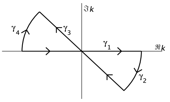
Figure 2.

First of all we prove that

Lemma 4.

$$\lim_{R\to+\infty}\frac{4a}{\pi}\int_{\gamma_{j}}h(k)e^{-ik^{2}t}dk=0\ \mbox{ for }\ j=2,4\,.$$

Proof.

Indeed, for $j=2$ (for instance), then $k=Re^{i\theta}$, $\theta\in[-\pi/4,0]$, and thus (remember that $\gamma_{2}$ is clock-wise oriented)

$$\frac{4a}{\pi}\int_{\gamma_{2}}h(k)e^{-ik^{2}t}dk=-\frac{4a}{\pi}\int_{-\pi/4}^{0}h(Re^{i\theta})e^{-iR^{2}te^{2i\theta}}Rd\theta$$

Hence

$$\left|\frac{4a}{\pi}\int_{\gamma_{2}}h(k)e^{-ik^{2}t}dk\right| \leq C\int_{-\pi/4}^{0}\left[1+\frac{e^{-2Ra\sin\theta}}{R^{3}}\right]e^{2R^{2}t\sin\theta\cos\theta}d\theta$$

$$\leq C\int_{-\pi/4}^{0}\left[1+\frac{e^{-2Ra\sin\theta}}{R^{3}}\right]e^{\sqrt{2}R^{2}t\sin\theta}d\theta\to 0\ \mbox{ as }\ R\to+\infty\,.$$

since $\cos\theta\geq\frac{\sqrt{2}}{2}$ for $\theta\in[-\pi/4,0]$. ∎

Therefore, we can conclude that

$$f_{0}(t) = \frac{4a}{\pi}e^{-i\pi/4}\int_{-\infty}^{+\infty}h(ke^{-i\pi/4})e^{-i(ke^{-i\pi/4})^{2}t}dk$$

$$= \frac{4a}{\pi}e^{-i\pi/4}\int_{-\infty}^{+\infty}h(ke^{-i\pi/4})e^{-k^{2}t}dk$$

$$= \frac{8a}{\pi^{5/2}t^{1/2}}e^{-i\pi/4}+\frac{2^{3/2}ia^{3}(\pi^{2}-8)(1+i)}{t^{3/2}\pi^{9/2}}+O(t^{-5/2})\ \mbox{ as }\ t\to+\infty$$

by Watson’s Lemma (see pg. 402 by [10]).  Lemma 3 is thus proved. ∎

Remark 8.

It is well known (see Lemma 7.10 at page 169 by [12]) that

$$\left[e^{-itH_{0}}\phi\right](x) = \frac{1}{\sqrt{2it}}e^{ix^{2}/4t}\widehat{\left(e^{iy^{2}/4t}\phi(y)\right)}\left(\frac{x}{2t}\right)$$

$$\sim \frac{1}{\sqrt{2it}}e^{ix^{2}/4t}\hat{\phi}(x/2t)$$

in norm as $t$ goes to infinity.  Then, when $\psi$ and $\phi$ coincide with the eigenvector $\psi_{1}$ an explicit calculation gives that

$$\hat{\psi}_{1}(\omega)=\sqrt{2\pi a}\frac{1+e^{i2\omega a}}{e^{i\omega a}(-4\omega^{2}a^{2}+\pi^{2})}\,.$$

Hence

$$\langle\psi_{1},e^{-itH_{0}}\psi_{1}\rangle = \int_{-a}^{+a}\sqrt{\frac{\pi}{it}}\cos(\pi x/2a)\frac{\left(1+e^{ixa/t}\right)e^{ix^{2}/4t}}{e^{ixa/2t}\left(\pi^{2}-a^{2}x^{2}/t^{2}\right)}dx$$

$$= \sqrt{\frac{\pi}{it}}\int_{-a}^{+a}\cos(\pi x/2a)\frac{\left(1+e^{ixa/t}\right)e^{ix^{2}/4t}}{e^{ixa/2t}\left(\pi^{2}-a^{2}x^{2}/t^{2}\right)}dx$$

$$\sim \sqrt{\frac{\pi}{it}}\int_{-a}^{+a}\cos(\pi x/2a)\frac{2}{\pi^{2}}dx=\frac{8a\sqrt{-\pi i}}{t^{1/2}{\pi}^{3}}$$

in agreement with Lemma 3.

4.2.2. Asymptotic behavior of $f_{r}(t)$ for large $t$

Lemma 5.

Let $\psi=\phi$ coinciding with the eigenvector $\psi_{1}$.  Then

$$f_{r}(t)=-\frac{8a}{\pi^{5/2}\sqrt{t}}e^{-i\pi/4}-\frac{2^{3/2}(1+i)a^{3}\left(\pi^{2}-8\right)}{\pi^{9/2}t^{3/2}}-\frac{2^{3/2}(1+i)a}{\pi^{5/2}t^{3/2}\alpha^{2}}+$$

$$\ \ -\sum_{m=1}^{\infty}\frac{\alpha\beta_{m}\ell(k_{1,-m})^{2}}{1+\alpha a\left(1+\frac{2k_{1,-m}}{i\alpha}\right)}e^{-ik_{1,-m}^{2}t}+O(t^{-5/2})$$

where $\beta_{m}$ is defined by (37).

Proof.

We recall (47), where the function $\ell(k)$ has been defined by (38) and where we observe that at the roots $k=\pm k_{1}=\pm\frac{\pi}{2a}$ of the denominator of $\ell(k)$ then

$$\lim_{k\to\pm k_{1}}\ell(k)=\frac{1}{8}\frac{\pi\pm 3i}{\pi}\,.$$

Furthermore, the integral converges because for large values of $k$ the integrand function behaves as the integrable (in absolute value) function $\frac{1}{k^{5}}$.  The integrand function has poles coinciding with the roots of $(2k+i\alpha)+i\alpha e^{2ika}$, that is at

$$k_{1,j}=\frac{i}{2a}\left[W_{j}(-a\alpha e^{a\alpha})-a\alpha\right]\,,\ j\in{\mathbb{Z}}\,.$$

Now, let $R>0$ be fixed and let (see Fig. 3)

$$\gamma=\gamma_{1}\cup\gamma_{2}\cup\gamma_{3}\cup\gamma_{4}$$

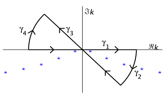
Figure 3. Asterisks denote the poles $k_{1,j}$, $j\in{\mathbb{Z}}$, of the integrand function in (47).

as in the proof of Lemma 3, where $R>0$ is such that $k_{1,j}\notin\gamma$.  Since the integrals along $\gamma_{2}$ and $\gamma_{4}$ go to zero as $R$ goes to infinity, as in Lemma 4, and from the Cauchy theorem it follows that

$$f_{r}(t)=I+II$$

where

$$I = -\frac{\alpha}{\pi i}\int_{\gamma_{3}}\frac{[\ell(k)]^{2}}{(2k+i\alpha)+i\alpha e^{2ika}}e^{-ik^{2}t}dk$$

$$= \frac{\alpha}{\pi i}\int_{{\mathbb{R}}}\frac{\ell(ke^{-i\pi/4})^{2}}{(2ke^{-i\pi/4}+i\alpha)+i\alpha e^{2ike^{-i\pi/4}a}}e^{-k^{2}t}e^{-i\pi/4}dk$$

$$= -\frac{8a}{\pi^{5/2}\sqrt{t}}e^{-i\pi/4}-\frac{2^{3/2}(1+i)a^{3}\left(\pi^{2}-8\right)}{\pi^{9/2}t^{3/2}}-\frac{2^{3/2}(1+i)a}{\pi^{5/2}t^{3/2}\alpha^{2}}+O(t^{-5/2})$$

by means of the Watson’s Lemma, and where the term II picks up the contribution due to the residue at the poles $k_{1,-m}$, $m=1,2,3,\ldots$, such that $|\Im k_{1,-m}|\leq|\Re k_{1,-m}|$:

$$II = -2{\alpha}\sum_{m=1}^{\infty}\beta_{m}\mbox{Res}\left[\frac{\ell(k)^{2}}{(2k+i\alpha)+i\alpha e^{2ika}}e^{-ik^{2}t}\right]_{k=k_{1,-m}}$$

$$= -2\alpha\sum_{m=1}^{\infty}\frac{\beta_{m}\ell(k_{1,-m})^{2}}{2+2\alpha a\left(1+\frac{2k_{1,-m}}{i\alpha}\right)}e^{-ik_{1,-m}^{2}t}$$

where $\beta_{m}=1$ if the pole $k_{1,-m}$ is inside the complex set enclosed by $\gamma$, and where $\beta_{m}=\frac{1}{2}$ if the pole $k_{1,-m}$ belongs to the border $\gamma$, otherwise $\beta_{m}=0$.  Lemma 5 is so proved. ∎

4.3. Proof of Theorem 1

In fact, the proof of Theorem 1 is nothing but the extension of the proof of Theorem 2 to the general case.  Indeed, the function $f_{\alpha}$ may be written as

$$f_{\alpha}(t)=\frac{1}{\pi i}\int_{{\mathbb{R}}}F_{\alpha}(k)e^{-ik^{2}t}dk$$

where

$$F_{\alpha}(k) = k\left[G_{0}(k)+g(k)G_{r}(k)\right]$$

and where $G_{0}(k)$, $G_{r}(k)$ and $g(k)$ are respectively defined by (40), (43) and (29).  Hence, by means of the Cauchy theorem and by making use of the same arguments given in the proofs of Lemma 4 and 5 it follows that

$$f_{\alpha}(t)=\frac{1}{\pi i}\left[\int_{{\mathbb{R}}}F_{\alpha}(ke^{-i\pi/4})e^{-k^{2}t}e^{-i\pi/4}dk-\frac{1}{2\pi i}\sum_{n=1}^{\infty}\beta_{n}\mbox{Res}\ \left[kg(k)G_{r}(k)\right]_{k=\sqrt{{\mathcal{E}}_{\alpha,n}}}e^{-i{\mathcal{E}}_{\alpha,n}t}\right]$$

where $\beta_{n}=1$ if the pole $k=\sqrt{{\mathcal{E}}_{\alpha,n}}$ is inside the complex set enclosed by $\gamma$, and where $\beta_{n}=\frac{1}{2}$ if the pole $k=\sqrt{{\mathcal{E}}_{\alpha,n}}$ belongs to the border $\gamma$, otherwise $\beta_{n}=0$.  We should remark that we can apply the arguments by Lemma 4 and 5 provided that the functions $G_{0}(k)$, $\ell_{j}(k)$ and $m_{j}(k)$, $j=1,2$, admits analytic extension in the sectors $\{z\in{\mathbb{C}}\ :\ \mbox{arg}(z)\in[-\pi/4,0]\}$ and that such extensions may be suitably controlled by $e^{-ik^{2}t}$ in the same domain.  These conditions are both fulfilled provided that the test functions $\phi$ and $\psi$ are well localized.  Furthermore, in the general case we have both families of complex poles (23) and (24).  Finally, Watson’s Lemma [10] gives that

$$\int_{{\mathbb{R}}}F_{\alpha}(ke^{-i\pi/4})e^{-k^{2}t}e^{-i\pi/4}dk=e^{-i\pi/4}\int_{0}^{+\infty}\left[F_{\alpha}(ke^{-i\pi/4})+F_{\alpha}(-ke^{-i\pi/4})\right]e^{-k^{2}t}dk$$

$$\ \ =\frac{1}{2}e^{-i\pi/4}\sum_{j=0}^{N}\frac{t^{-(j+1)/2}}{j!}\Gamma\left(\frac{j+1}{2}\right)\left.\frac{d^{j}\left[F_{\alpha}(ke^{-i\pi/4})+F_{\alpha}(-ke^{-i\pi/4})\right]}{dk^{j}}\right|_{k=0}+O\left(t^{-(N+2)/2}\right)$$

$$\ \ =e^{-i\pi/4}\sum_{s=0}^{N}\frac{t^{-(2s+1)/2}}{2s!}\Gamma\left(\frac{2s+1}{2}\right)\left.\frac{d^{2s}F_{\alpha}(ke^{-i\pi/4})}{dk^{2s}}\right|_{k=0}+O\left(t^{-(N+2)/2}\right)$$

where a straightforward calculation gives that

$$F_{\alpha}(0)=0$$

for any $\alpha>0$.  Theorem 1 is thus proved.

Remark 9.

In fact, we could assume a weaker condition about the test functions $\phi$ and $\psi$; that is would be enough that

$$|\phi(x)|,\,|\psi(x)|\leq ae^{-bx^{2}}\,,\ x\in{\mathbb{R}}$$

for some $a,b>0$.

Appendix A The Lambert function

Here, we collect from [3] some basic properties of the Lambert function.  The Lambert function, denoted by $W(z)$, is defined to be the function satisfying the equation

$$W(z)e^{W(z)}=z\,,\ z\in{\mathbb{C}}\,.$$

This function is a multivalued analytic function.  The principal branch, denoted by $W_{0}(z)$, is analytic at $z=0$ and its power series expansion is given by

$$W_{0}(z)=\sum_{n=1}^{\infty}\frac{(-n)^{n-1}}{n!}z^{n}\,.$$

In particular $W_{0}(0)=0$.  This series has radius of convergence $1/e$.

In fact, if we denote $W_{m}(z)$, $m\in{\mathbb{Z}}$, all the branches of the Lambert function then we have the following picture:

• $W_{0}(z)$ is the only branch containing the interval $(-1/e,+\infty)$.  It has a second-order branch point at $z=-1/e$ and the branch cut is $(-\infty,-1/e]$.

• $W_{1}(z)$ and $W_{-1}(z)$ share the branch point at $z=-1/e$ with $W_{0}(z)$ and furthermore they also have a branch point at $z=0$.  Then, each of them has a double branch cut: $(-\infty-1/e]$ and $(-\infty,0]$.  By means of a suitable choice of the functions on the top of the branch cuts thus $W_{0}(z)$ and $W_{-1}(z)$ are the only branches of the Lambert function that take real values.

• All the other branches $W_{m}(z)$, $m\in{\mathbb{Z}}\setminus\{0,\pm 1\}$, have only the branch cut $(-\infty,0]$, similarly to the branches of the logarithm.

Among the properties of the Lambert function we recall the following ones:

• Symmetry conjugate property: $W_{m}(\bar{z})=\overline{W_{-m}(z)}$.

• Asymptotic expansion for large argument: for large $z$ we have that

  $$W_{m}(z)=\ln(z)+2\pi im-\ln\left[\ln(z)+2\pi im\right]+\sum_{k=0}^{+\infty}\sum_{j=1}^{+\infty}c_{kj}\frac{\ln^{j}\left[\ln(z)+2\pi im\right]}{\left[\ln(z)+2\pi im\right]^{j+k}}$$ (48)

  where

  $$c_{kj}=\frac{(-1)^{k}}{j!}\left[\begin{array}[]{c}k+j\\ k+1\end{array}\right]$$

  where $\left[\begin{array}[]{c}k+j\\ k+1\end{array}\right]$ is a Stirling cycle number of first kind.

References

- [1] S. Albeverio, F. Gesztesy, R. Hoegh-Krohn, and H. Holden, Solvable models in quantum mechanics, (Berlin: Springer, 1988).
- [2] F. Chevoir, and B. Vinter, Scattering assisted tunneling in double barriers diode: scattering rates and valley current, Phys. Rev. B 47 (1993) 7260–7274 (1993).
- [3] R.M. Corless, G.H. Gonnet, D.E. Hare, D.J. Jeffrey, and D.E. Knuth, On the Lambert W function, Adv. Comp. Math. 5 329-359 (1996).
- [4] D.C. Dobson, F. Santosa, S.P. Shipman, and M.I. Weinstein, Resonances of a potential well with a thick barrier, SIAM J. Appl. Math. 73 1489-1512 (2013).
- [5] C. Ferrari, and H. Kovarik, On the exponential decay of magnetic Stark resonances, REp. Math. Phys. 56 197-207 (2005).
- [6] Gottfried K., and T.M. Yan, Quantum Mechanics: fundamentals, Graduate texts in contemporary physics, edition, (Springer: New York, 2003).
- [7] E.M. Harrell II, Perturbation Theory and Atomic Resonances since Schrödinger’s Time, published as pp. 227-248 in: P. Deift, F. Gesztesy. P. Perry, and W. Schlag, eds., Spectral Theory and Mathematical Physics: A Festschrift in Honor of Barry Simon’s 60th Birthday, Proceedings of Symposia in Pure Mathematics 76.1. Providence: American Mathematical Society, 2007.
- [8] I.W. Herbst, Exponential Decay in the Stark Effect, Commun. Math. Phys. 75 197-205 (1980).
- [9] H. Kovaric, and A. Sacchetti, A nonlinear Schrödinger equation with two symmetric point interactions in one dimension, J. Phys. A: Math. Theor. 43 155205 (2010).
- [10] Yu.V. Sidorov, M.V. Fedoriuk, and M.I. Shabunin, Lectures on the theory of functions of a complex variable, (MIR Publ.: Moscow 1985).
- [11] B. Simon, Resonances in n-body quantum systems with dilatation analytic potentials and the foundations of time-dependent perturbation theory,, Ann. Math. 97, 247-274 (1973).
- [12] G. Teschl, Mathematical Methods in Quantum Mechanics, with applications to Schrödinger operators, Graduate Studies in Mathematics (AMS: 2009)
- [13] R. Weder, Estimates for the Schrödinger Equation on the Line and Inverse Scattering for the Nonlinear Schrödinger Equation with a Potential, J. of Funct. Anal. 170, 37-68 (2000).
- [14] M. Zworski, Resonances in Physics and Geometry, Notices Amer. Math. Soc. 46 319-328 (1999).