The HIPASS survey of the Galactic plane in Radio Recombination Lines

Abstract

We present a Radio Recombination Line (RRL) survey of the Galactic Plane from the Hi Parkes All-sky Survey and associated Zone of Avoidance survey, which mapped the region $l=196\degr$ – $0\degr$ – $52\degr$ and $|b|\leq 5\degr$ at 1.4 GHz and 14.4 arcmin resolution. We combine three RRLs, H168$\alpha$, H167$\alpha$, and H166$\alpha$ to derive fully sampled maps of the diffuse ionized emission along the inner Galactic plane. The velocity information, at a resolution of 20 km s^-1, allows us to study the spatial distribution of the ionized gas and compare it with that of the molecular gas, as traced by CO. The longitude-velocity diagram shows that the RRL emission is mostly associated with CO gas from the molecular ring and is concentrated within the inner 30° of longitude. A map of the free-free emission in this region of the Galaxy is derived from the line-integrated RRL emission, assuming an electron temperature gradient with Galactocentric radius of $496\pm 100$ K kpc^-1. Based on the thermal continuum map we extracted a catalogue of 317 compact ($\stackrel{{\scriptstyle<}}{{{}_{\sim}}}$15 arcmin) sources, with flux densities, sizes and velocities. We report the first RRL observations of the southern ionized lobe in the Galactic centre. The line profiles and velocities suggest that this degree-scale structure is in rotation. We also present new evidence of diffuse ionized gas in the 3-kpc arm. Helium and carbon RRLs are detected in this survey. The He line is mostly observed towards Hii regions, whereas the C line is also detected further away from the source of ionization. These data represent the first observations of diffuse C RRLs in the Galactic plane at a frequency of 1.4 GHz.

1 INTRODUCTION

Radio Recombination Lines (RRLs) have been widely used in astrophysics, especially as probes of the physical conditions of the line emitting plasma and Hii regions. From the observation of a single transition, the electron temperature of the gas can be determined by comparing the energy radiated by the line to that of the underlying thermal free-free continuum. This remains one of the most accurate methods to determine the electron temperature. The central velocity of the line and its width give information about the systematic and turbulent motions of the gas.

In this paper we present the RRL data from the Hi Parkes All-Sky Survey (HIPASS, Staveley-Smith et al. 1996) and associated Zone of Avoidance Survey (ZOA, Staveley-Smith et al. 1998), which cover the Galactic plane accessible from Parkes, $l=196\degr$ – $0\degr$ – $52\degr$, and $|b|\leq 5\degr$. The first results from the analysis of the three H$\alpha$ RRLs, H168$\alpha$, H167$\alpha$, and H166$\alpha$, for a smaller section of the Galactic plane are given in Alves et al. (2010, 2012) (hereafter Paper i and Paper ii respectively). Calabretta, Staveley-Smith & Barnes (2014) used the full HIPASS and ZOA datasets to produce a map of the 1.4 GHz continuum emission in the southern sky.

RRLs arising from low density gas are relatively weak, with temperatures of tens to a hundred mK at frequencies near 1 GHz, thus about 1 per cent of the thermal continuum brightness in the Galactic plane (see Section 3). So far studies of the diffuse ionized gas have been performed by pointed observations towards positions in the inner plane free from strong Hii regions (e.g., Gottesman & Gordon 1970, Jackson & Kerr 1971, Heiles, Reach & Koo 1996, Baddi 2012). Here we present the first contiguous survey of RRL emission in the plane of the Galaxy, suitable for a comprehensive study of the diffuse ionized medium. We note that similar surveys, at the same frequency and at higher angular and spectral resolution, are underway with the Arecibo telescope (SIGGMA, Liu et al. 2013) and the Very Large Array (THOR, Bihr et al. 2013). The former will cover part of the first quadrant and a region of the anti-centre, $l=30\degr$ – $75\degr$ and $l=175\degr$ – $207\degr$ respectively, within $2\degr$ of the Galactic plane, whereas the latter will map the region $l=15\degr$ to $67\degr$, $|b|\leq 1\degr$.

Our previous RRL study of the region $l=20\degr$ – $44\degr$ and $|b|\leq 4\degr$ revealed a width of the emission at velocities corresponding to the Sagittarius and Scutum spiral arms of $0$ .${}^{\circ}85\pm 0$ .${}^{\circ}03$ and $0$ .${}^{\circ}78\pm 0$ .${}^{\circ}01$ respectively (Paper ii). This is equivalent to a $z$-thickness of $96\pm 4$ pc and thus slightly broader than 74 pc, the width of the distribution of OB stars, the progenitors of Hii regions (Bronfman et al., 2000). This implies that the ionizing radiation from the OB stars is not fully absorbed in the dense molecular clouds in which they are born, but escapes into the surrounding lower density medium, which it ionizes.

The inner Galaxy has been mapped and studied over a wide range of frequencies, from radio to infra-red (e.g., Haynes, Caswell & Simons 1978; Haslam et al. 1982; Reich 1982; Reich et al. 1990; Miville-Deschênes & Lagache 2005; Stil et al. 2006; Jarosik et al. 2011; Sun et al. 2011). Paladini et al. (2005) and Sun et al. (2011) have used some of these data to separate the thermal and non-thermal emission at radio frequencies by exploiting the difference in their brightness temperature spectral indices. Even if the free-free spectrum is well known, uncertainties in the synchrotron spectral behaviour and degree of polarization, as well as in the zero levels of the different surveys, limit this method. However, a more direct approach is possible thanks to the RRL data. These provide a measure of the free-free emission that, when compared with the total continuum at the same frequency, enables the separation of the synchrotron component (Paper ii).

One obvious advantage of RRLs over other thermal emission tracers is that they are not attenuated by interstellar dust along the line of sight and can thus be interpreted directly. This provides an unambiguous estimate of the Emission Measure (${\rm EM}=\int n_{e}^{2}d\ell$), which is valuable for the study of the electron density distribution. The RRL emission from ionized hydrogen gas can be expressed in terms of the integral over spectral line temperature, $T_{\rm L}$, as

$$\int T_{\rm L}d\nu=1.92\times 10^{3}T_{\rm e}^{-1.5}{\rm EM}$$ (1)

where $\nu$ is the frequency (kHz), $T_{\rm e}$ is the electron temperature in K and the emission measure EM is in cm^-6 pc (Rohlfs & Wilson, 2000). The corresponding continuum emission brightness temperature is

$$T_{\rm b}=8.235\times 10^{-2}a(T_{\rm e},\nu)T_{\rm e}^{-0.35}\nu^{-2.1}_{\rm GHz}(1+0.08){\rm EM}$$ (2)

where $a(T_{\rm e},\nu)$ is a slowly varying function of the electron temperature and frequency (Mezger et al., 1967; Dickinson, Davies & Davis, 2003; Draine, 2011) and the $(1+0.08)$ factor represents the additional contribution to $T_{\rm b}$ from helium. Thus, the underlying free-free emission can be obtained from the integrated RRL as follows

$$T_{\rm b}=\frac{1}{6.985\times 10^{3}}a(T_{\rm e},\nu)(1+0.08)T_{\rm e}^{1.15}\nu_{\rm GHz}^{-1.1}\int{T_{\rm L}dV}$$ (3)

where $V$ is in  km s^-1. This equation is valid for $\alpha$ transitions (i.e., one-level transitions), in Local Thermodynamic Equilibrium (Rohlfs & Wilson, 2000).

The present data allow the determination of a fully-sampled map of the free-free emission in the inner Galaxy, thus providing an even better sampling of the spiral arms. Such a map is valuable not only for separating thermal and non-thermal emission, allowing synchrotron objects to be studied at 1.4 GHz, but also for star formation studies since it includes both the individual and bright Hii regions and the extended ionized emission surrounding them. Recently these RRL data have been used as part of an inversion method that separates dust emission in the Herschel bands associated with atomic, molecular and ionized gas in a $2\degr\times 2\degr$ region centred at $(l,b)=(30\degr,0\degr)$ (Traficante et al., 2014). These data are unique in that they provide the velocity information of the ionized component necessary for this work and until now unavailable in the Galactic plane. Tibbs et al. (2012) used the RRL data towards the Anomalous Microwave Emission (AME) object RCW175 to confirm its thermal radio component and also to compare the velocity of the ionized gas with that of other gas tracers. Furthermore, the separation of the several foreground emission components from Cosmic Microwave Background observations, such as those delivered by the Planck satellite, can be improved significantly using the results reported here. An estimate of the free-free emission in the Galactic plane is a major input to disentangle the other components at radio frequencies. Planck Collaboration (2014b) used the free-free map of Paper ii to isolate the AME in the Galactic plane region $l=20\degr$ – $40\degr$and $|b|\leq 4\degr$. The same data have also been used by Planck Collaboration (2014a) to remove the ionized emission from the millimetre channels of Planck and thus to study and characterise the emission of interstellar dust.

This paper is organised as follows. Section 2 describes the RRL survey, data reduction and calibration. In Section 3 we present the RRL maps and study the spatial distribution of the ionized gas, namely how it compares with that of the molecular gas. We also show evidence of carbon RRL emission from the diffuse medium in the Galactic plane. Section 4 presents a list of Hii regions extracted from the free-free map, along with their flux densities at 1.4 GHz, angular sizes and line velocities. Section 5 focuses on the Galactic centre region, where we study the structure of the ionized degree-scale lobe and present observations of diffuse emission from the 3-kpc arm. Finally, we conclude with a summary of the present work in Section 6.

2 THE RRL SURVEY AND DATA

The HIPASS and ZOA surveys are described in Staveley-Smith et al. (1996, 1998). These searched for Hi-emitting galaxies in the velocity range $-1280$ to 12700 km s^-1 using the Parkes 21-cm multibeam receiver. Within the 64 MHz bandwidth there are three RRLs: H168$\alpha$, H167$\alpha$ and H166$\alpha$ at 1374.601, 1399.368 and 1424.734 MHz, respectively, which are combined and used to recover the thermal emission. The HIPASS survey covers the sky south of $\delta=+25$ .${}^{\circ}5$. The multibeam receiver has 13 beams, each with two linear polarizations (Stokes $I$ only), set on a hexagonal grid with a mean observing beam width of 14.4 arcmin full width at half maximum (FWHM). The survey is divided into 15 zones and the scans are taken at constant right ascension, in declination strips of 8° separated by 7 arcmin. Hence, each of the 13 beams mapped the sky at slightly below the Nyquist rate. The ZOA deep survey scanned at constant Galactic latitude and each $8$ .${}^{\circ}5$ longitude scan is separated by 1.4 arcmin. It covers most of the Galactic plane accessible from Parkes, $l=196\degr$ – $0\degr$ – $52\degr$ and $|b|\leq 5\degr$, and is divided into 27 zones. The latitude coverage was extended to $|b|\leq 10\degr$ for $l=332\degr$ – $0\degr$ – $36\degr$ and $|b|\leq 15\degr$ for $l=348\degr$ – $0\degr$ – $20\degr$. The footprint of the receiver on the sky has a width of $1$ .${}^{\circ}7$, thus each scan maps an area slightly greater than $8$ .${}^{\circ}5\times 1$ .${}^{\circ}7$. The multibeam correlator cycle is 5 s and the scan rate is 1° min^-1, therefore each scan has 100 integrations. The HIPASS/ZOA frequency coverage is from 1362.5 to 1426.5 MHz centred on 1394.5 MHz and is divided into 1024 channels spaced by 62.5 kHz, or 13.4 km s^-1 for the H167$\alpha$ line. The total integration time is 450 s per beam for the HIPASS survey and 2100 s per beam for the five times deeper ZOA survey. This results in a typical rms (root mean square) noise of 13 mJy beam^-1 and 6 mJy beam^-1 for the HIPASS and ZOA surveys, respectively.

The results presented in this paper use a combination of the HIPASS and ZOA datasets for the Galactic plane region $l=196\degr$ – $0\degr$ – $52\degr$ and $|b|\leq 5\degr$. Table 1 lists the relevant observing parameters. The data analysis techniques and properties of the final maps are described below.

Table 1: Summary of the HIPASS/ZOA RRL survey parameters.

Beams	13
	1 central, 6 inner ring, 6 outer ring
Beam FWHM	14.0, 14.1, 14.5 arcmin
Beam ellipticity	0.00, 0.03, 0.06
Gridded beam FWHM	14.4 arcmin
Polarizations	2 orthogonal linear
	(Stokes $I$ only)
Longitude coverage	$l=196\degr$ – $0\degr$ – $52\degr$
Latitude coverage	$|b|\leq 5\degr$
RRLs included:
H168$\alpha$	1374.601 MHz
H167$\alpha$	1399.368 MHz
H166$\alpha$	1424.734 MHz
Scan rate	1° min-1
Integration time	5 s
Channel separationa	13.4 km s-1
Velocity resolution	20 km s-1
rms noiseb	4.5 mK (6.4 mJy beam-1)
$T_{\rm b}/S$	$0.70\pm 0.07$ K /(Jy beam-1)

^a Equivalent to 62.5 kHz at the frequency of the H167$\alpha$ line.
^b Typical rms noise in the stacked spectra, at a velocity resolution of 20 km s^-1, along the Galactic plane.

2.1 Data analysis

In this section we describe the main aspects of the data analysis, which have been presented in Paper ii. There are two additional steps, related to the continuum ripple removal and gridding of the data, which are detailed in Calabretta, Staveley-Smith & Barnes (2014), since the reduction of the HIPASS/ZOA spectral data follows closely that of the continuum.

The spectra generated by the multibeam correlator are dominated by the system bandpass, which is corrected using the tsysmin algorithm (Paper ii) in the livedata software (Barnes et al., 2001). tsysmin, which was developed to recover extended emission in the Galactic plane, locates the $n$ ($=10$ in this work) integrations in each scan for which the median value of the system temperature is a minimum and, for each spectral channel, takes the median value over the same integrations as the bandpass correction. Other effects in the spectra such as spectral ringing due to strong Hi Galactic emission, baseline ripple, and non-linearities in the receiver and amplifier system are not eliminated in this process. Spectral ringing is reduced by smoothing the spectra using the Tukey filter (Tukey, 1967). Baseline ripple is caused by single or multiple reflections of radiation from strong continuum sources between the dish and the receiver. Even though its pattern is not purely sinusoidal, due to reflections from the feed legs as well, it can be well reproduced and removed from the spectra. In addition to the ripple, a rise in the bandpass response towards low-frequencies is observed in the spectra of strong continuum sources, proportional to their strength. These two effects are corrected via a scaled template method: a normalized continuum baseline signature is determined for each beam and polarization using a large subset of the HIPASS/ZOA data, scaled accordingly and removed from each spectrum after bandpass correction. The Sun and many other strong continuum sources in the Galactic plane when seen in the beam sidelobes may generate off-axis ripple. This ripple has no characteristic signature, is often quite complex and may vary rapidly. Calabretta, Staveley-Smith & Barnes (2014) describe a method to filter this ripple, mainly being of use for point sources. It was not applied in the present RRL data reduction in order to avoid possible side effects on the extended emission.

After bandpass correction and calibration, the three RRLs are extracted from each 1024 channel spectrum, shifted by the correct fractional number of channels by Fourier interpolation and then stacked. The errors introduced by stacking the lines in frequency space rather than in velocity space are less than 2 per cent of the channel width. The three lines are stacked using a weighted mean, where the weights are proportional to the square root of the bandpass response measured at each line’s rest frequency. The weights are 0.35, 0.39 and 0.26 for the H168$\alpha$, H167$\alpha$ and H166$\alpha$; the lower H166$\alpha$ weight is due to the Gibbs ringing close to the strong Hi line (figure 2 in Paper i). Averaging of the RRLs improves the signal-to-noise of the final line by a factor of $\sim\sqrt{3}$. The number of channels extracted was set to 51, the maximum number accommodating the proximity of the H166$\alpha$ line to the edge of the band, and is equivalent to an LSR (local standard of rest) velocity range of $\pm 335$ km s^-1.

The stacked RRL spectra are then gridded using gridzilla (Barnes et al., 2001) into 4 arcmin pixels. The spectrum at each pixel is generated from the weighted median of the stacked spectra within a cut-off radius of 6 arcmin. The weight for each input spectrum is based on its angular distance from the pixel. Even though the weighted median estimation is non-linear, it is robust against RFI (radio frequency interference) and other time-variable sources of emission such as the Sun, and it also produces a gridded beam that is very close to Gaussian with 14.4 arcmin FWHM. However, one effect of median gridding is that the flux density scale differs depending on the source size (Paper ii). This problem has now been overcome by iterative gridding (Calabretta, Staveley-Smith & Barnes, 2014) using a gain factor of 1.2 in order to minimize the number of iterations and consequent increase in the rms noise. Simulations indicate that a gain factor of 1.2 recovers the peak height and integrated flux of sources of various sizes within 1 per cent, with a negligible effect in the final beam FWHM.

This procedure is applied to the ZOA and the HIPASS datasets separately, which are combined by correcting the ZOA data for a latitude-dependent offset and averaging both datasets, giving five times more weight to the ZOA survey (Paper ii). The data are further Tukey smoothed, hence the spectral resolution is degraded from 16 km s^-1 to 20 km s^-1.

2.2 Calibration

Figure 1: T-T plots for (a) the Rosette nebula, (b) W35, and (c) W40, showing the correlation between the HIPASS/ZOA and the Jonas, Baart & Nicolson (1998) surveys. The HIPASS/ZOA data have been smoothed to 20 arcmin resolution and extrapolated from 1.4 to 2.3 GHz. The vertical dotted lines indicate the values above which the linear fit, shown by the solid lines, is performed.

Table 2: The first 10 entries of the list of 317 Hii regions in the range $l=196\degr$ – $0\degr$ – $52\degr$ and $|b|\leq 5\degr$, extracted from the thermal continuum map of Fig. 7 using SExtractor. The full catalogue is available online. Column 1 numbers each object; columns 2 and 3 are the Galactic coordinates; columns 4 and 5 give the angular size of the source, where $\theta_{a}$ and $\theta_{b}$ are the measured values $a$ and $b$ deconvolved with the 14.4 arcmin beam; $p$ indicates that the object is less than 10 arcmin in size; column 6 is the PA measured counterclockwise between the semi-major axis of the source and the longitude axis; columns 7 and 8 give the peak and total flux density at 1.4 GHz; column 9 gives the RRL central velocity from a one- or two-component Gaussian fit; column 10 gives the internal flags generated by SExtractor^a; column 11 gives general remarks on the source^b.

Number	$l$	$b$	$\theta_{a}$	$\theta_{b}$	PA	$S_{\rm p}$	$S$	$V$	Flag a	Notesb
	($\degr$)	($\degr$)	(arcmin)	(arcmin)	($\degr$)	(Jy beam-1)	(Jy)	(km s-1)
$1$	$1.14$	$0.01$	$14.9$	$p$	$-45$	$20.4\pm 4.0$	$29.3\pm 5.8$	$-20.5$	$0$	C [1]
$2$	$2.21$	$0.34$	$p$	$p$	—	$8.0\pm 1.6$	$8.0\pm 1.6$	$4.7$	$2$	—
$3$	$2.44$	$0.17$	$17.2$	$p$	$-19$	$8.0\pm 1.7$	$12.4\pm 3.5$	$4.3$	$2$	—
$4$	$3.18$	$-0.03$	$17.2$	$14.5$	$5$	$11.7\pm 2.9$	$25.8\pm 6.9$	$4.0$	$0$	—
$5$	$4.33$	$0.20$	$13.6$	$p$	$7$	$12.3\pm 2.8$	$16.9\pm 4.2$	$4.4$	$0$	[1]
$6$	$4.47$	$-0.11$	$p$	$p$	—	$9.7\pm 2.7$	$9.7\pm 2.7$	$9.6$	$0$	[1]
$7$	$4.73$	$0.17$	$p$	$p$	—	$8.4\pm 2.5$	$8.4\pm 2.5$	$7.4$	$0$	—
$8$	$5.18$	$-0.16$	$p$	$p$	—	$5.7\pm 2.1$	$5.7\pm 2.1$	$5.6$	$0$	—
$9$	$5.24$	$0.17$	$14.4$	$p$	$11$	$6.6\pm 2.5$	$9.3\pm 4.0$	$9.7$	$2$	[1]
$10$	$5.84$	$-0.37$	$12.6$	$p$	$4$	$33.1\pm 5.9$	$44.0\pm 8.0$	$12.5$	$2$	W28 [1]

^a Flag parameter: 2 - the source was originally blended with another one; 8 - the source is truncated owing to its proximity to the image boundary. ^b These are taken from Paladini et al. (2003) and follow the definitions given by Kuchar & Clark (1997) to define if a source is: C, in a complex field; S, with a strong source nearby; X, with a strong source nearby ($<10$ Jy), radio or optical counterpart. The value within the square brackets corresponds to the number of sources in the Paladini et al. catalogue that match a given source in this survey.

During observations, the system temperature was calibrated against a high-quality noise diode switched in and out of the signal path. The diode itself was calibrated periodically against flux density calibrators. Gaussian fits to the peak heights of the source 1934-638 (14.9 Jy at 1420 MHz) and Hydra A (40.6 Jy at 1395 MHz), resulted in a mean calibration factor of 1.09 (1.11 and 1.07 for 1934-638 and Hydra A respectively; Calabretta, Staveley-Smith & Barnes 2014).

A detailed knowledge of the beam pattern and of the sky brightness distribution is required in order to convert the data correctly to absolute temperature units in the presence of both compact and extended emission (e.g., Rohlfs & Wilson 2000). However, both these quantities are difficult to measure and thus the conversion is usually performed in the full beam scale, using a single value across the whole map. The full beam corresponds to the integral of the observed beam pattern out to a large radius, whereas the main beam is measured within the first sidelobes (Jonas, Baart & Nicolson, 1998).

In Paper ii we converted the data to the main beam scale following the Rayleigh-Jeans relation for a Gaussian FWHM of 14.4 arcmin at the frequency of the H167$\alpha$ line, obtaining a value of $T_{\rm b}/S=0.84$ K /(Jy beam^-1). This scale is appropriate for compact sources and overestimates the emission from sources more extended than the beam. The above value compares with 0.80  K /(Jy beam^-1), used in Hi observations of extended objects with the Parkes telescope (Staveley-Smith et al., 2003), and which is appropriate for the somewhat higher mean efficiency of the inner seven beams. A lower value of about 0.57 K /(Jy beam^-1) is expected for the outer beams. An alternative to the use of theoretical conversion factors is the comparison with other data sets. Calabretta, Staveley-Smith & Barnes (2014) converted the 1.4 GHz continuum map by correlating the HIPASS/ZOA data with an existing map at the same frequency but lower resolution, 35.4 arcmin, and which is calibrated in the full beam brightness scale for a very extended beam of $7\degr$ (Reich, 1982; Reich & Reich, 1986; Reich, Testori & Reich, 2001). The authors derive an empirical factor of 0.44 K /(Jy beam^-1), 30 per cent lower than the theoretical value of 0.57 K /(Jy beam^-1). This discrepancy is likely due to power on intermediate and large scales ($\stackrel{{\scriptstyle>}}{{{}_{\sim}}}7\degr$), dominating the cross-plot of the HIPASS/ZOA versus the Reich et al. data used to derive the conversion factor.

In this work we perform an independent analysis by comparing the HIPASS/ZOA continuum data with that from the 2.3 GHz survey by Jonas, Baart & Nicolson (1998), at 20 arcmin resolution. The authors quote an uncertainty in the full beam scale of less than 5 per cent, for a beam efficiency of 69 per cent. Even if the two surveys cover a similar area of the sky, we need to perform the comparison over restricted regions, since the datasets have to be extrapolated to the same frequency using a fixed spectral index. We focus on regions dominated by thermal emission, thus located in the Galactic plane, and within the limits of the RRL survey, selecting three Hii regions: the Rosette nebula (G206.2-2.1), W35 (G18.5+2.0), and W40 (G28.8+3.5). These are three of the few objects in the area under study that are well isolated and outside the Galactic plane (see Fig. 7).

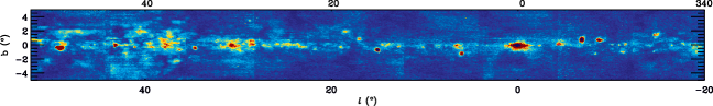
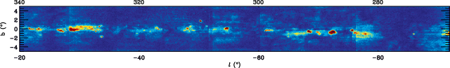
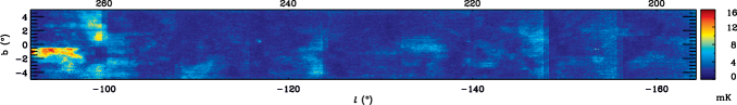
Figure 2: Map of the rms noise per channel, estimated using the emission-free ends of each spectrum (see text). The longitude coverage of the survey is divided into three sections: $l=340\degr$ – $0\degr$ – $52\degr$, $l=268\degr$ – $340\degr$, and $l=196\degr$ – $268\degr$. The typical rms noise in the Galactic plane is 4.5 mK, increasing by nearly a factor of 10 towards some of the brightest Hii regions. Note the two longitude labels above and below each panel.

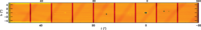
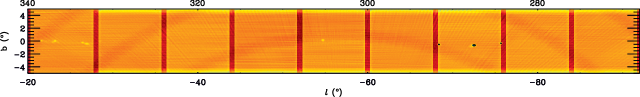
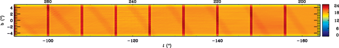
Figure 3: Beam coverage map given by the sum in quadrature of beam weights used to produce the final data cube and maps. One unit corresponds to one independent boresight observation. The longitude coverage of the survey is divided into three sections as in Fig. 2. Typical values are around 18, increasing to about 22 where ZOA zones overlap. The saturated pixels have values below 10 (within the black contour). This map illustrates the striations along the HIPASS and ZOA scan directions, as well as the overlap regions between the different zones.

Fig. 1 shows the resulting T-T plots. The HIPASS/ZOA continuum emission is extrapolated from 1.4 to 2.3 GHz using a spectral index $\beta=-2.1$, where $T\propto\nu^{\beta}$ (Dickinson, Davies & Davis, 2003; Draine, 2011), and smoothed from 14.4 to 20 arcmin resolution. We select regions of $4\degr\times 4\degr$ centred on the Rosette and $2\degr\times 2\degr$ centred on W35 and W40. The maps are gridded to a common pixel size of 8 arcmin and all of the pixels for each region are shown in Fig. 1. The correlation between the two data sets gives conversion factors of $0.68\pm 0.10$, $0.69\pm 0.05$, and $0.72\pm 0.08$ K /(Jy beam^-1) for the Rosette, W35, and W40 Hii regions respectively, where the uncertainties correspond to the scatter of the points relative to the best fit line. The correlation is performed using the points above a given threshold value in temperature, shown by the vertical dotted line in each panel of Fig. 1. This threshold is applied in order to exclude background emission, which also includes synchrotron emission at these frequencies and latitudes (Paper ii). The background level is estimated by fitting a Gaussian profile with a constant term to the 2.3 GHz maps. The increase in the conversion factor from one object to the other is likely related to their angular size: W40 has a FWHM of about $\sim 10$ arcmin compared to $\sim 40$ and $\sim 60$ arcmin for the W35 and Rosette Hii regions, respectively (Table 2). The Rosette and W35 Hii regions are representative of emission broader than the 14.4 arcmin beam and extended over scales of $\stackrel{{\scriptstyle<}}{{{}_{\sim}}}1\degr$, whereas W40 has a size comparable to the beam, hence a factor closer to 0.80 K /(Jy beam^-1). The estimated conversion factors are consistent within their uncertainties, with a mean value of $T_{\rm b}/S=0.70\pm 0.03$ K /(Jy beam^-1). If we vary the background levels by 1 K, the mean calibration factor changes by 0.02 K /(Jy beam^-1); this difference is included in the 4 per cent uncertainty on $T_{\rm b}/S$.

We use the above value of 0.70 K /(Jy beam^-1) to convert the RRL data into brightness temperature, given that the instrument and data are the same and that the reduction of the HIPASS/ZOA continuum data is similar to that of the spectral lines. We can also estimate the conversion factor using the free-free map derived from the RRL integrated intensity (using Eq. (3) and described in Section 3.4) as we did with the HIPASS/ZOA total continuum. The mean conversion factor obtained from the analysis of the same three regions is $T_{\rm b}/S=0.68\pm 0.11$ K /(Jy beam^-1), which is consistent with that derived above using the total continuum. The higher uncertainty results partly from the larger scatter of the points, associated with a higher noise level, but also from the uncertainty on the electron temperature, which will be discussed in Section 3.4.

Finally, we adopt $T_{\rm b}/S=0.70$ K /(Jy beam^-1) along with a conservative calibration uncertainty of 10 per cent, considering that both the 1.09 factor above and the brightness temperature conversion are based on only two and three sources respectively. We note that for a direct comparison of the RRL data with the HIPASS/ZOA continuum data, the latter need to be corrected by a factor of 1.6, the ratio between the conversion factor found here (0.70  K /(Jy beam^-1)) and that derived in Calabretta, Staveley-Smith & Barnes (2014) (0.44  K /(Jy beam^-1)).

2.3 Final data cube

The final $216\degr\times 10\degr\times 670$ km s^-1 data cube covers the $l$-range $196\degr$ – $0\degr$ – $52\degr$, $|b|\leq 5\degr$ and $V_{\rm LSR}=\pm 335$ km s^-1. Fig. 2 shows the spectral rms noise map, for the velocity resolution of 20 km s^-1. We estimate the standard deviation of each spectrum using its emission-free ends, which correspond to 38 out of the 51 channels once we allow for the RRL emission to spread within the conservative range of $\pm 85$ km s^-1 about its peak velocity (Section 3.3). The central RRL velocity is found using a three-point quadratic fit around the brightest peak (miriad task moment, Sault, Teuben & Wright 1995). The rms noise per channel in the cleanest regions of the survey is 2.8 mK. However, the typical value in the Galactic plane, as well as close to the regions where individual $8\degr(l)\times 10\degr(b)$ ZOA scans overlap, is 4.5 mK or 6.4 mJy beam^-1. At the location of some of the brighest continuum sources, the spectral noise reaches 20 – 40 mK; this is due to the stronger baseline ripple effect and spectral ringing from Galactic Hi emission. Nevertheless, the regions of highest rms noise also have high ($>3$) signal-to-noise spectra.

The vertical discontinuities visible in the spectral rms maps are also seen in some of the RRL channel maps that are presented in Section 3.1 (Fig. 5). The overlap of individual scans is clearer in the beam coverage map of Fig. 3, which shows the square root of the sum of squares of the beam weights used in producing the spectral cube. One unit in this map corresponds to one independent boresight observation. Over these regions and especially outside the Galactic plane, some of the channel maps show negative values. This is likely due to differences in the baseline levels, related to the bandpass correction (Section 2.1). This effect is, nevertheless, at a level of about 2 times the rms noise. Striations are seen along the direction of the HIPASS scans, which cross the Galactic plane at various angles, in some of the velocity channels and zones, e.g., $l\sim 320\degr$ and $V=26.8$ km s^-1, or $l\sim 270\degr$ and $V=-80.3$ km s^-1 (Fig. 5). This is a low level effect, of the order of $\sim$1 – 2 mK.

Figure 4: Comparison between the HIPASS/ZOA RRL data and those from the surveys of (a) Hart & Pedlar (1976), (b) Lockman (1976), and (c) Heiles, Reach & Koo (1996). The quantity plotted, with the corresponding error bars, is the RRL integrated intensity in units of K  km s^-1. The dashed lines indicate equality and the solid lines correspond to the linear fit between the different data sets. There are 51, 43, and 208 points in panels (a), (b), and (c), respectively.

Some of the pixels in the maps are blanked as the corresponding data are affected by sources strong enough to saturate the receiver electronics. There are 129 pixels affected, seen in the beam coverage map of Fig. 3 with values below 10 (e.g., 63 pixels in the Galactic centre, 21 pixels in M17 G15.1-0.7).

The spectral negatives, which originate from the bandpass distortions (Section 2.1), are seen at the position of some strong sources in Fig. 5. They appear in the velocity channels adjacent to those corresponding to the peak emission of the object. For example, the Hii region M8 G6.0-1.2 peaks at $V\sim 0$ km s^-1 and a negative of about $10$ per cent of its peak temperature is seen at the same position, at $V=53.6$ km s^-1. Stronger spectral negatives are produced by an interfering signal at $V\approx-130$ km s^-1, which significantly affects a large part of the data, especially in the fourth quadrant of the Galactic plane. In this longitude range, $l\sim 270\degr$ – $330\degr$, the interfering signal is at a similar velocity to that expected from helium and carbon RRLs (Section 3.5). However this effect is small when observing low in the north (i.e., at $l\sim 30^{\circ}$). The effects of the interference can be seen around $l=312\degr$ at $V=-147.3$ km s^-1 and $l=288\degr$ at $V=-133.8$ km s^-1 (visible in the longitude-velocity diagram of Fig. 6). The former is probably associated with the radio galaxy Centaurus B, $(l,b)=(309.7\degr,1.7\degr)$, where a negative spike of about 200 mK is detected. The same negatives are present in the spectra of neighbouring Hii regions, nevertheless at $\sim 90$ km s^-1 away from their emission peak, which is at $V\sim-50$ km s^-1. The spectral negatives at $l\sim 288\degr$ are seen mostly around the three close-by bright Hii regions that have saturated pixels (Fig. 5). Similar to the previous case, this distortion of the spectra by strong continuum sources does not seem to affect the peak of the hydrogen lines that are about 100 km s^-1 away. This can, however, affect the helium and carbon spectra (Section 3.5).

In summary, the data show some striations and discontinuities, which are large-scale artifacts close to the noise level, as well as more significant defects, the spectral negatives that originate from bandpass distortions. Nevertheless, as will be shown in the next section, such artifacts do not affect the quality of the data within the assumed calibration uncertainty of 10 per cent.

2.4 Comparison with previous RRL observations

The accuracy of the present data can be checked by comparison with previous RRL observations. We consider three surveys made at a similar frequency and with comparable angular resolutions, but with different telescopes and observing techniques. Hart & Pedlar (1976) and Lockman (1976), hereafter HP76 and L76 respectively, measured the H166$\alpha$ line at positions along the first quadrant of the Galactic plane. HP76 used the Mk II telescope, with a beam FWHM of $31\times 33$ arcmin, whereas the L76 observations were performed at an angular resolution of 21 arcmin with the 43 m NRAO telescope. Heiles, Reach & Koo (1996), hereafter HRK96, targeted hundreds of positions mostly towards the inner Galaxy, but restricted to $|b|>0$ .${}^{\circ}6$, with the NRAO and the 26 m HCRO telescope with 36 arcmin beam. We use the data from the HCRO telescope, which observed most of the positions primarily at the H165$\alpha$ and H167$\alpha$ lines.

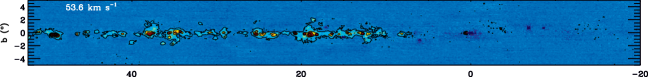
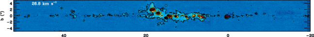
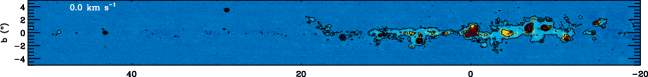
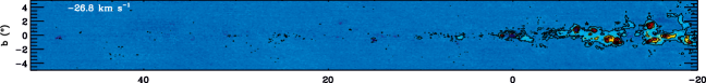
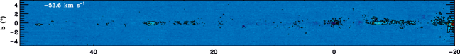
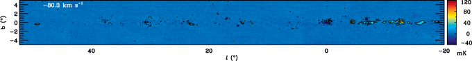
Figure 5: Maps of the RRL emission at different velocity channels, as indicated in the top left corner of each panel. The longitude coverage of the survey is divided into three sections as in Fig. 2. Contours are at 10, 50, 90, 190, 290, and 390 mK.

The results are shown in Fig. 4, where we compare the RRL integrated intensities in order to take into account the different velocity resolutions of the surveys. The HIPASS data are smoothed to the lower angular resolutions of 32, 21, and 36 arcmin to match the observing beams of HP76, L76, and HRK96, respectively; the data are further regridded to pixel sizes of 9, 6, and 10 arcmin. The uncertainties in the HIPASS intensities follow from the propagation of the spectral noise (Fig. 2) to the line integral, as described in Section 3.3. We also add in quadrature the 10 per cent systematic uncertainty, associated with the brightness temperature calibration (Section 2.2). The correlation between the HIPASS and the three different surveys gives linear slopes of $1.2\pm 0.2$, $1.08\pm 0.04$, and $1.03\pm 0.06$, for HP76, L76, and HRK96, respectively. The linear fits take into account the uncertainties in both abscissa and ordinate. These results indicate that the present RRL data are consistent with previous observations at the 10 per cent level, and thus give confidence in the overall accuracy and calibration of the current survey.

3 The ionized Galactic disk

In this section we present the RRL emission at 1.4 GHz in the plane of the Galaxy and discuss its three-dimensional distribution.

3.1 RRL maps

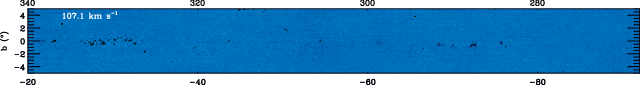
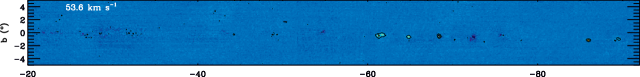
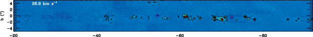
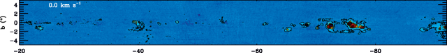
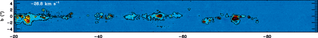
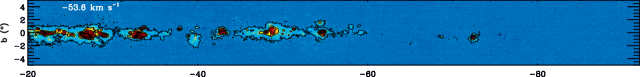
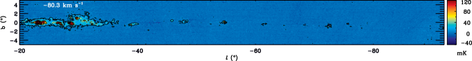
Figure 5:

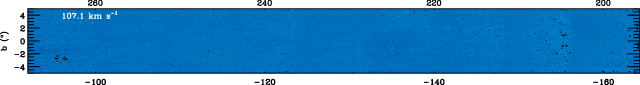
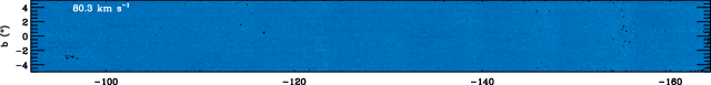
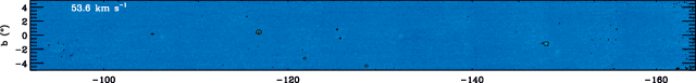
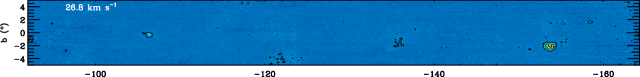
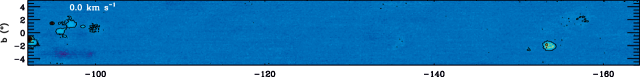
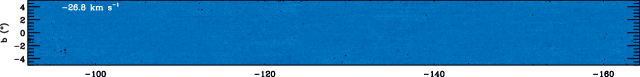
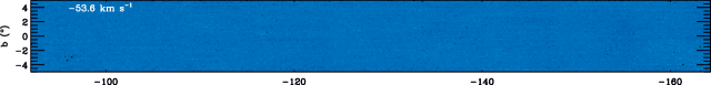
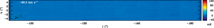
Figure 5:

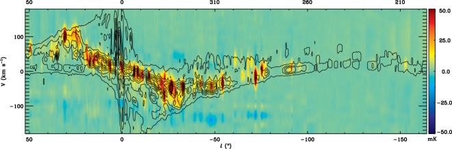
Figure 6: Longitude-velocity diagram of the RRL brightness temperature integrated over a strip of $4\degr$ in latitude, centred in the Galactic plane. The spectra are averaged every $0$ .${}^{\circ}5$ in longitude. The contours show the distribution of the CO emission from the survey of Dame, Hartmann & Thaddeus (2001); they are at every 300 mK from 25 to 1825 mK. Both the RRL and the CO emission follow the velocity pattern of the spiral arms, with a wider velocity distribution for the molecular gas.

The RRL emission at eight velocity channels, between $V=-80.3$ and 107.1 km s^-1 is shown in Fig. 5. Individual Hii regions can be identified in the different maps, as well as the extended emission around and between them. A list of Hii sources is presented in Section 4. Beyond the inner Galactic plane, or at $|l|\geq 60\degr$, there are only a few isolated complexes of Hii regions visible in the map, namely RCW57 G291.6-0.4, the Carina Nebula G287.4-0.6, RCW49 G284.3-0.3, and RCW38 G267.9-1.0, in the Carina spiral arm, as well as the Rosette Nebula G206.4-2.3 in the Perseus spiral arm. On the other hand, emission at all velocities is visible across the inner Galaxy, consistent with the fact that the bulk of star formation is occurring in the inner two spiral arms of the Galaxy (Wood & Churchwell, 1989; Bronfman et al., 2000). At velocities $V\stackrel{{\scriptstyle<}}{{{}_{\sim}}}30$ km s^-1 the emission is broader in latitude since it arises from the nearby Local and Sagittarius/Carina spiral arms. Emission further away from us, in the Scutum/Norma spiral arms, has higher velocities and a narrower latitude distribution. This is not the case in the central $2\degr\times 2\degr$ of the Galaxy, where the RRL emission is at velocities close to zero. However, this line-emitting gas is not necessarily foreground or local gas but is also in the Galactic centre (GC) region (Law et al., 2009). This region will be further discussed in Section 5.

3.2 Longitude-velocity distribution

The distribution of the RRL velocity as a function of longitude is shown in Fig. 6, where we can see the change from positive to negative velocities as we go from quadrants I to IV. The negative (forbidden) velocities in quadrant I, for example associated with the Hii complex W43 at $l=30\degr$ and $V\sim-50$ km s^-1, originate from helium and carbon RRLs (Section 3.5). The negatives seen in the diagram are associated with bandpass distortions by strong continuum sources, as described in Section 2.3, thus they appear at the same longitude as the strong emission but at a different velocity.

The highest absolute values of velocity observed at $|l|\sim 30\degr$ corresponds to the lines of sight crossing the tangent of the Scutum-Norma spiral arm, at a distance of about 4 kpc (using a solar Galactocentric distance of 8.5 kpc, Kerr & Lynden-Bell 1986). The tangent point of the Sagittarius arm at $l\sim 50\degr$ is not well covered by the RRL survey, nevertheless there is clear emission associated with the W51 complex at $V\sim 60$ km s^-1. There is also RRL emission associated with the quadrant IV of the Carina spiral arm, at $l=300\degr$ and $V\sim 30$ km s^-1.

The contours in Fig. 6 trace the CO emission detected in the survey of Dame, Hartmann & Thaddeus (2001). The CO spectra are averaged within the same $0$ .${}^{\circ}5(l)\times 4\degr(b)$ areas as the RRL data, and smoothed from their initial resolution of 2 km s^-1 to 20 km s^-1. The diagram clearly shows that the RRL emission is mostly associated with the CO gas from the molecular ring, the region of high CO emission within $|l|\stackrel{{\scriptstyle<}}{{{}_{\sim}}}30\degr$. Furthermore, the fact that star formation is not present in every molecular complex across the Galaxy (e.g., Evans 1991) is well illustrated by the narrower velocity range covered by the RRL emission, compared to the wider velocity spread of the CO emission at a given longitude. There are peaks in RRL emission that do not have an associated CO peak, e.g., at $l=284\degr$ and $V\sim 0$ km s^-1, $l=287$ .${}^{\circ}4$ and $V\sim-20$ km s^-1, or $l=336$ .${}^{\circ}7$ and $V\sim-10$ km s^-1. The second example corresponds to the Carina nebula, a giant Hii region with a large number of massive stars (Smith & Brooks, 2008). It is thus possible that the parent molecular cloud has been disrupted by the powerful stellar feedback from several generations of stars.

The 3-kpc expanding arm (Cohen & Davies, 1976) is seen in CO (Dame & Thaddeus, 2008) emission within $|l|\stackrel{{\scriptstyle<}}{{{}_{\sim}}}10\degr$ and at negative velocities, close to the first contour in Fig. 6. High signal-to-noise RRL emission associated with the 3-kpc arm is detected, but not seen in the longitude-diagram due to the large (4°) latitude band used in averaging the spectra. Non-circular motions in the GC with a large spread of velocities, up to $\sim 200$ km s^-1, have been observed, both in molecular and atomic tracers (Burton & Hekkert, 1985; Burton, 1988; Dame, Hartmann & Thaddeus, 2001). However, as mentioned in the previous section, we find that the RRL emission towards the GC is mostly at velocities near zero, which is expected for circular motions nearly perpendicular to the line of sight. Spectra towards the GC will be presented in Section 5, which also show the negative velocity component arising from the 3-kpc expanding arm.

3.3 RRL integrated intensity

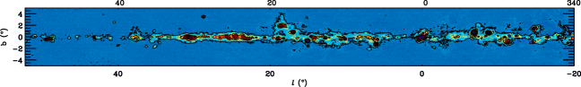
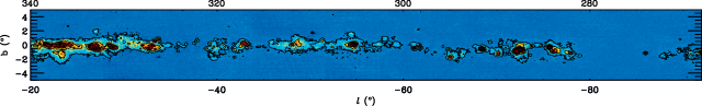
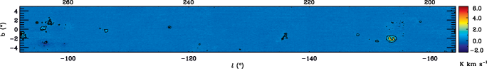
Figure 7: Map of the total RRL integrated emission in units of K km s^-1 and at a resolution of 14.4 arcmin. The contours correspond to the free-free brightness temperature distribution at 1.4 GHz (Section 3.4); they are at 1.5, 7.5, 13.5, 25, 45, 65, and 85 K. The longitude coverage of the survey is divided into three sections as in Fig. 2.

The total RRL integrated emission for the Galactic plane region $l=196\degr$ – $0\degr$ – $52\degr$ and $|b|\leq 5\degr$ is shown in Fig. 7. This represents the first fully-sampled map of ionized emission in this region of the Galaxy. The conversion of the line integral into a free-free brightness temperature is presented in the next section.

The map of Fig. 7 is in units of K km s^-1 and at a resolution of 14.4 arcmin. The velocity integration range is set differently for spectra with peak temperature above and below $3\sigma_{\rm T}$, where $\sigma_{\rm T}=4.5$ mK is the typical rms noise measured in the Galactic plane (Section 2.3). This threshold roughly defines the ridge of emission within the first contour of Fig. 7, where the spectra are integrated over 170 km s^-1 about their peak velocity. Such a velocity range is wide enough to include the emission allowed by Galactic rotation along the plane, without including emission from He/C RRLs (Section 3.5). In the case where the line is below $3\sigma_{\rm T}$ the central velocity is assumed to be 0 km s^-1, the velocity of local emission, and each spectrum is summed within a narrower range of 92 km s^-1. Finally, the data are clipped at $-3\sigma$, i.e., channels with temperature below $-3$ times the spectral noise (Fig. 2) are not included in the line integrated emission. We note that if we use a constant clip value of $-3\sigma_{\rm T}$, the resulting RRL integrated emission is about 3 per cent higher in the brightest regions of the inner Galaxy (within the first contour of Fig. 7).

The maximum and minimum of the map are $-4$ and 38 K km s^-1, respectively, and the rms noise measured away from the Galactic plane ($|b|\stackrel{{\scriptstyle>}}{{{}_{\sim}}}3\degr$) is $0.1$ K km s^-1. The fraction of pixels with RRL integrated emission below $-0.3$ K km s^-1 is only 0.4 per cent. The dynamic range of the map, defined as the ratio between the maximum intensity and the noise level, is 380.

3.4 Free-free emission at 1.4 GHz

The thermal continuum emission is obtained as described in Section 1 (Eq. (3)), namely through the RRL integral and a value for the electron temperature. The free-free emission is shown by the contours of Fig. 7, which follow the RRL integrated emission.

The electron temperature of Hii regions is known to vary with the Galactocentric radius $R_{\rm G}$ (Shaver et al., 1983; Paladini, Davies & DeZotti, 2004): $T_{\rm e}$ decreases towards the Galactic centre due to its higher metal content. In Paper ii we studied 15 Hii regions within $l=20\degr$ – $44\degr$ and $|b|\leq 4\degr$ and found that:

$$T_{\rm e}[\rm K]=(3609\pm 479)+(496\pm 100)R_{\rm G}[\rm kpc]$$ (4)

using the Fich, Blitz & Stark (1989) rotation curve, with $\Theta_{\odot}=220$ km s^-1 and $R_{\odot}=8.5$ kpc, the rotation velocity and Galactocentric distance of the Sun, respectively $R_{\rm G}=\frac{221.64R_{\odot}}{\Theta_{\odot}+V/{\rm sin}(\ell)+0.44R_{\odot}}$. (Kerr & Lynden-Bell, 1986). This results in electron temperatures about 5 – 10 per cent higher than those from both Shaver et al. (1983) and Paladini, Davies & DeZotti (2004). Furthermore, we have shown in Paper ii  that for that same region of the Galaxy, the electron temperature of the diffuse free-free emission is similar to that of the individual Hii regions. Therefore, we apply Eq. (4) to every pixel in the RRL spectral cube where the peak temperature is above $3\sigma_{\rm T}$, as defined in Section 3.3, using the central line velocity to estimate $R_{\rm G}$. Note that for each spectrum the central velocity corresponds to the brightest peak; when multiple peaks are present, meaning when there is more than one velocity component along the line of sight, $T_{\rm e}$ should be estimated based on the relative brightness of each of the peaks. Nevertheless, neglecting the contribution of different velocity components does not significantly affect the derived value of $T_{\rm e}$ within the typical uncertainty of 1000 K, associated with Eq. (4). The typical value of electron temperature obtained along the Galactic plane is 6000 K. For the low signal-to-noise pixels, for which we ascribed the local velocity of 0 km s^-1, we set $T_{\rm e}=7000$ K, the mean electron temperature in the Solar neighbourhood (Shaver et al. 1983; Paladini, Davies & DeZotti 2004, Paper ii). The exact value of $T_{\rm e}$ in these pixels is not crucial since their emission is within the noise level. Due to the complexity of the GC region and the difficulty of deriving the Galactocentric distance based on the radial velocity at these longitudes, we do not apply Eq. (4) within $l=354\degr$ – $0\degr$ – $4\degr$ but set $T_{\rm e}$ to a constant value of $T_{\rm e}=6000$ K to obtain a smooth variation of the electron temperature with longitude. However, we note that lower values, $T_{\rm e}\stackrel{{\scriptstyle<}}{{{}_{\sim}}}4000$ K, have been determined towards the GC (Law et al., 2009), which are consistent with the result of Eq. (4) for $R_{\rm G}=0$.

For typical values of $T_{\rm e}=6000\pm 1000$ K, the uncertainty in the derived free-free continuum emission is 20 per cent. If a constant electron temperature of 7000 K is used throughout the whole Galactic plane, then the free-free map is simply a scaled version of the RRL integrated emission, with 1.0 K km s^-1 equivalent to 2.8 K of brightness temperature at 1.4 GHz (Eq. (3)). The minimum and maximum of the free-free map are $-9$ and 116 K, respectively, and the rms noise measured away from the Galactic plane is 0.3 K. Less than 0.3 per cent of the pixels have emission below $-0.9$ K.

Figure 8: Average spectra, $12\times 12$ arcmin², measured in a diffuse line of sight (a), next to the bright Hii region W34 (b). The dashed vertical lines indicate the expected velocities of the He and C RRLs, relative to the H line. The two component Gaussian fit to each spectrum is given by the solid line. In panel (b), the dotted curve corresponds to the second order fit performed to correct the baseline.

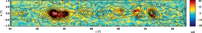
Figure 9: Map of the RRL emission at $V=-55$ km s^-1, the expected velocity of C line emission from the Scutum spiral arm. The contours correspond to the H RRL at $V=94$ km s^-1 and are at every 25 mK from 10 to 410 mK. The two labels in the map show the positions at which the spectra of Fig. 8 are measured.

3.5 Helium and Carbon RRLs

The 168$\alpha$ – 166$\alpha$ RRLs from helium and carbon are also detected in this survey. They are separated from the H line by $-122.1$ and $-149.5$ km s^-1 respectively, relative to the H RRL velocity scale. As the velocity separation between the He and C RRLs is similar to the spectral resolution of 20 km s^-1, the two lines are usually blended in these data. The C RRL arises from colder gas lying in front of the continuum source, in photodissociation regions (Balick, Gammon & Hjellming, 1974; Dupree, 1974). Stimulated emission by the background source results in line temperatures that are orders of magnitude above that expected from the carbon abundance (Goldberg & Dupree, 1967). If the cold gas is not associated with the Hii region that induces the line enhancement but is at a different velocity, then the C RRL is correspondingly shifted in velocity and can be separated from the He line (Paper ii). C RRL emission can also arise from diffuse gas (Kantharia & Anantharamaiah, 2001), ionized by the interstellar UV radiation field.

The spectra of Fig. 8 show the He/C RRLs measured towards the W43 G30.7+0.0 complex. Fig. 8 (a) is the spectrum for a diffuse line of sight, $0$ .${}^{\circ}6$ away from the centre of the bright Hii region. Gaussian fits give a width of $29\pm 2$ km s^-1 for the H line and $19\pm 6$ km s^-1 for the RRL at the velocity expected for the C line; the narrower width of the latter is consistent with a line arising from a cooler medium. The ratio between the C and H RRL amplitudes is $17\pm 2$ per cent. An example of the distortion of the bandpass (Section 2.1) by the strong continuum source W43 is provided by the spectrum of Fig. 8 (b). After a second order polynomial fit around the carbon central velocity, we find a large line width of $48\pm 5$ km s^-1, indicating the presence of both He and C RRLs. Their combined amplitude of about 110 mK results in a ratio of 18 per cent relative to the H line. The ionization energy of atomic carbon is 11.3 eV, lower than that of H, 13.6 eV, and much lower than that of He, 24.6 eV. Our observations are consistent with the fact that He RRLs should be detected towards the Hii region, where the stellar radiation is sufficiently high, whereas C RRLs can also be observed further away from the ionizing sources.

The channel map of Fig. 9 shows the line emission at $V=-55$ km s^-1 for the $l$-range $21\degr$ – $34\degr$ and within 1° of the Galactic plane, where the H RRL peaks at about 94 km s^-1. Emission at the C RRL velocity is seen across the whole W43 complex as well as towards the W41 (G23.4+0.0) and W42 (G25.3-0.1) Hii regions, where the C line is brighter outside the continuum peaks. Diffuse Cii gas is best detected at low frequencies, $\stackrel{{\scriptstyle<}}{{{}_{\sim}}}1$ GHz, where C RRLs from the Galactic plane have been observed mostly within $l<20\degr$, both in emission and absorption (Erickson, McConnell & Anantharamaiah, 1995; Kantharia & Anantharamaiah, 2001). The decrease in the background continuum, thus in the stimulated emission, along with the low angular resolution of past surveys, are responsible for the limited number of detections of C RRLs beyond $l=20\degr$ (Roshi & Anantharamaiah, 2000; Roshi, Kantharia & Anantharamaiah, 2002).

Here we present the first observations of C RRLs at 1.4 GHz from diffuse gas along the Galactic plane. The Galactic plane region shown in Fig. 9 is one of the cleanest in which to identify the C RRL as it shows only one H RRL component, consistent with the velocity of the Scutum spiral arm. In the fourth quadrant of the Galaxy, specifically within $l=270\degr$ – 330°, negative spikes at $\sim-130$ km s^-1 corrupt the spectra at or near the expected velocity of the He/C RRLs (Section 2.3). However, these lines are observed towards other objects across the whole coverage of this survey and can be investigated.

Studies of the morphology and physical conditions of Cii regions can be pursued using the present data, combined with previous surveys, not only of C RRLs at different frequencies but also of other cold gas tracers such as Hi and C⁺.

4 A catalogue of Hii regions

In Paper ii we presented a list of 48 Hii sources in the region $l=20\degr$ – $44\degr$, $|b|\leq 4\degr$, with sizes, flux densities, and velocities as measured from the RRL free-free map. All those objects are known and have been observed by many continuum as well as RRL surveys (e.g., the source compilation by Paladini et al. 2003 and the recent RRL survey by Anderson et al. 2011). Here we extend this list to include all the thermal sources detected in the present free-free map. This list gives the source parameters, free of any synchrotron contamination, which can occur when analysing total continuum surveys, and due to its resolution of $\sim 14$ arcmin, it includes the more extended emission around and between features. An additional advantage of RRL detections is that for each source we have a velocity measurement, thus its distance to the Sun can be obtained for diffuse and compact Hii regions.

4.1 Source detection

We follow the same approach as in Paper ii to create a catalogue of Hii regions from this survey, using the source extractor algorithm SExtractor (Bertin & Arnouts, 1996) and adjusting its main input parameters such as background mesh, detection threshold and filter function. These are tuned to recover not only the bright sources easily visible in the map, but also weaker objects, whose spectra are also checked to confirm whether they do indeed correspond to a real signal. The background is estimated in every $1\degr\times 1\degr$ region, utilising an iterative clipping of the background histogram until convergence at $\pm 3\sigma$ around its median. We then apply a $3\times 3$ deg² median filter to create a smoother background map. We note that the typical size of the detected sources is $\sim 0$ .${}^{\circ}1$, thus significantly smaller than the background mesh size. The source detection is performed on the input free-free map after filtering with a Mexican Hat filter of width 12 arcmin, similar to the beam size. If a source extends beyond 3 pixels, or $3\times 4$ arcmin, and is above the detection threshold of 2$\sigma$, where $\sigma=0.3$ K (Section 3.4), it is considered a detection. The source size is measured from the second-order moment map and given in terms of $a$ and $b$, the ellipse major and minor axes. We compute the flux density $S$ of each source assuming a Gaussian profile as follows

$$S=S_{\rm p}\frac{a\times b}{fwhm^{2}}$$ (5)

where $S_{\rm p}$ is the peak flux and $fwhm$ is the beam FWHM of 14.4 arcmin. The peak flux is measured at the central position of each object from the background-subtracted free-free map.

4.2 Properties of the catalogue

Figure 10: Cumulative counts as a function of the (a) flux density and (b) size. The solid line corresponds to the 317 sources listed in Table 2 and the dashed line to the 285 objects detected when using a Mexican Hat filter of 20 arcmin width.

The first 10 rows of the catalogue of sources extracted from the free-free map are reported in Table 2. This table lists the Galactic coordinates, angular size, position angle, peak and integrated flux density, and central velocity of each object. The broadening of the beam is difficult to measure for small sources, especially if they are also weak. We consider that a source is unresolved when its size is smaller than 10 arcmin, which implies an angular broadening of 3 arcmin relative to the 14.4 arcmin beam. We take this conservative value, which is much larger than the variation of the FWHM of the individual beams (0.5 arcmin, Table 1), to account also for beam modelling uncertainties: the typical uncertainty on the fitted sizes is 2 arcmin, which follows from both the noise level in the free-free map, as well as the uncertainty on the background estimation. Therefore, unresolved sources are indicated with the symbol $p$ whenever the observed size is below 17.5 arcmin. Further, if the area of a source ($a\times b$) is smaller than the beam area ($fwhm^{2}$), $S=S_{\rm p}$. The position angle (PA) is undefined in such cases. The uncertainty on the peak flux takes into account the spectral noise of the RRL data as well as the rms of the background map estimated by SExtractor. We do not include the systematic uncertainty associated with the electron temperature nor the overall calibration uncertainty of the survey. The uncertainty on the flux densities is about 25 per cent.

Table 2 includes sources that have a signal-to-noise ratio on the flux density above 2. Fig. 10 (a) shows the integral count $N(>S)$ for the 317 objects as a function of the flux density $S$. The catalogue has a lower limit of 3 Jy and is complete down to 5 Jy at a 95 per cent level. This is partly due to source confusion, meaning the difficulty of resolving the Galactic plane structure into individual objects, as well as to the sensitivity of the survey. The cumulative distribution of the size $\theta$ of the Hii regions is shown in Fig. 10 (b), where $\theta=(\theta_{a}+\theta_{b})/2$ and $\theta_{a}$ and $\theta_{b}$ are the measured values $a$ and $b$ deconvolved with the beam. We compare these results with those obtained when using a Mexican Hat filter of larger width, 20 arcmin. Fig. 10 shows that both the completeness and lower limit of the flux densities and sizes are not affected, meaning that using a filter function of width larger than the beam FWHM does not necessarily recover fainter sources. On the other hand, the larger convolving beam results in larger sizes for the 285 detected objects. As a consequence, the flux densities are also higher. The total flux of the 317 Hii regions in Table 2 is 121 212 Jy beam^-1, 73 per cent of which arises from the inner Galaxy, $|l|\leq 50\degr$. The contribution of the individual sources to the total free-free emission (Fig. 7), which amounts to 415 371  Jy beam^-1, is about 30 per cent. This result is similar to that found in Paper ii  for the smaller longitude range analysed. We note that some of the sources in the list are part of large Hii complexes (e.g., W42, W47) or are usually identified as a single object (e.g., sources 110 – 114 correspond to the Rosette Nebula). Moreover, due to the presence of saturated pixels at their centres, the 6 Hii regions marked in Fig. 3 are not recovered from the free-free map, and thus not listed in Table 2.

The last column of Table 2 gives general remarks on the object as well as its commonly used name(s). These notes are taken from the Paladini et al. (2003) Master Catalogue. Since the Paladini et al. catalogue is a compilation of results from several surveys with beam sizes generally smaller than the HIPASS 14.4 arcmin FWHM, we consider a match if the distance between objects from both catalogues is within 7.5 arcmin, about half of the beam FWHM. A total of 195 objects has one or more spatially corresponding source in the Master Catalogue. The central RRL velocity listed in Table 2 is derived from a one- or two-component Gaussian fit to the average $12\times 12$ arcmin² spectrum measured at the position of each object. There are 374 discrete H RRL components from the 317 sources in the list. We also check our estimates of the RRL velocity against those in the Master Catalogue, when available. The agreement is better than 6.7 km s^-1, or half of a channel, for 84 per cent of the objects with counterparts in the Paladini et al. list. Due to the difference in angular resolution between these surveys, the flux densities also differ: the values found in our work can be a factor of 3 – 5 times higher than those given in the Master Catalogue, after scaling from 2.7 to 1.4 GHz with a flux spectral index $\alpha=-0.1$ ($S\propto\nu^{\alpha}$, Dickinson, Davies & Davis 2003, Draine 2011).

The present catalogue lists 50 objects within the region $l=20\degr$ – $44\degr$, $|b|\leq 4\degr$, compared to the 48 included in the Hii region list of Paper ii. This difference involves objects that have a peak flux below 15 Jy beam^-1, thus below 3 times the completeness limit of the survey. The flux densities in both catalogues agree within the errors; the mean value of the ratio between the flux densities from this work and from Paper ii is 1.3, when considering the 16 sources that have a peak flux above 15 Jy beam^-1. The discrepancy follows from a combination of factors: (i) data reduction, especially concerning the iterative gridding used here, which mostly affects the flux density of the smaller sources; (ii) data analysis, we have followed a different method to integrate the lines and produce the free-free map; (iii) the calibration has also changed relative to Paper ii; (iv) some of the sizes fitted by SExtractor are somewhat higher, which increases the flux densities.

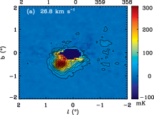
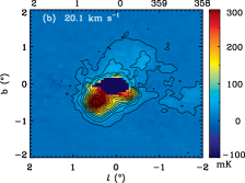
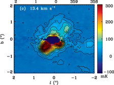
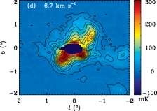
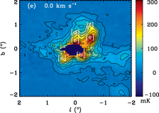
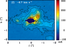
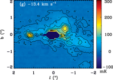
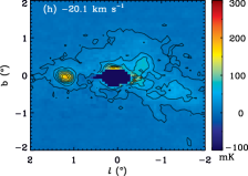
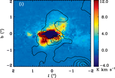
Figure 11: Channel maps of the RRL emission towards the GC region at several velocities, from panels (a) to (h). The southern part of the lobe is seen to peak at positive velocities, whereas the northern part is brightest at $V\sim 0$ km s^-1. The contours are at every 25 mK from 10 to 410 mK. We note that the central pixels in these maps are blanked due to the saturation of the receiver electronics by the strong GC continuum emission (Section 2.3). The labels in panel (e) are at the positions where the spectra of Fig. 12 are taken. Panel (i) shows the RRL integrated emission map of the GC region with contours from the velocity-integrated H$\alpha$ emission; these are at every 50 R from 25 to 225 R.

5 The Galactic centre

In this section we present the RRL data towards the GC region. These are the first fully-sampled observations of the ionized gas in RRL emission, which reveal a southern counterpart to the northern GC lobe previously detected at radio frequencies (Section 5.1). We also present evidence of diffuse ionized gas in the expanding 3-kpc arm (Section 5.2).

Figure 12: Average spectra, $12\times 12$ arcmin², taken at positions in the GC lobe, as indicated in Fig. 11 (e). Panels (a) and (b) correspond to the southern part of the lobe, (c) and (d) to the east northern ridge, and (e) and (f) to the west northern ridge. Gaussian fits to the spectra are shown.

5.1 The southern lobe

The degree-scale lobe seen towards the GC has been studied by Law et al. (2009) using several RRL observations between 4.56 and 5.37 GHz. This structure was first noted in a continuum survey at 10 GHz by Sofue & Handa (1984), who suggested that the lobe was of thermal origin, possibly the result of an energetic outflow phenomenon. The detection of RRL emission by Law et al. (2009) confirmed the thermal nature of the lobe, which is described as two vertical edges near $(l,b)=(0$ .${}^{\circ}0,0$ .${}^{\circ}5)$ and $(l,b)=(359$ .${}^{\circ}4,0$ .${}^{\circ}5)$, connected by a cap at $b\sim 1\degr$, thus north of the Galactic plane. These pointed observations with the Green Bank Telescope (GBT) focused on the ridges as well as on an horizontal strip from $l=359$ .${}^{\circ}25\rightarrow 0$ .${}^{\circ}25$ at $b=0$ .${}^{\circ}45$ and provided important information on the temperature and density of the ionized gas in this structure: the line-emitting gas has low velocity, $|V|\stackrel{{\scriptstyle<}}{{{}_{\sim}}}10$ km s^-1, and narrow widths, $\Delta V\sim 9-14$ km s^-1. Here we provide the first fully sampled map of the ionized GC lobe, which shows not only the known northern structure but also a southern counterpart detected for the first time at radio frequencies.

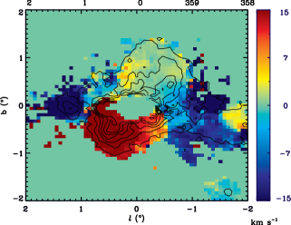
Figure 13: Map of the velocity at peak of the RRL emission towards the inner $4\degr\times 4\degr$ of the Galaxy. The GC southern lobe is seen at velocities of $\sim 15$ km s^-1, whereas the northern part is at $V\sim 0$ km s^-1. The contours correspond to the RRL integrated emission (Fig. 11 (i)) and are at every 2 K km s^-1 from 1 to 11 K km s^-1.

Channel maps at some relevant velocities are shown in Fig. 11. The two ridges and cap are brightest in Fig. 11 (e), at $V\sim 0$ km s^-1, whereas the southern extension of the lobe is brighter in Fig. 11 (c), at $V\sim 13$ km s^-1. Therefore, besides the small velocity gradient of $\sim 10$ km s^-1 measured by Law et al. (2009) in the northern lobe, there is also a difference with relation to the southern counterpart. This will be further discussed below (Fig. 12). In Fig. 11 (g) the north-west ridge of the lobe is still visible, as well as the Hii region G1.13-0.07. Fig. 11 (i) shows the contours of the H$\alpha$ integrated emission towards the GC region overlaid on that of the RRLs. The H$\alpha$ data are from the all-sky map composed by Finkbeiner (2003), which is based on the Southern H-Alpha Sky Survey Atlas (SHASSA) survey (Gaustad et al., 2001) in this region of the sky; these data are smoothed from their initial angular resolution of 6 arcmin to 14.4 arcmin. The fact that the optical line does not follow the thermal emission from the lobes, indicates that these structures are indeed at a large distance from us and hence are absorbed by the dust along the long line-of-sight towards the GC. The H$\alpha$ emission peaks at around $(l,b)=(359$ .${}^{\circ}75,-0$ .${}^{\circ}35)$, presumably a local Hii region, which is brightest in the RRL channel map of Fig. 11 (c). The second H$\alpha$ peak at $(l,b)=(358$ .${}^{\circ}3,-1$ .${}^{\circ}8)$ corresponds to the RRL emission seen at $V=0$ km s^-1 in Fig. 11 (e).

Spectra taken at positions across the GC lobe are shown in Fig. 12. These are $12\times 12$ arcmin² average spectra, to which a single or double component Gaussian is fitted. Figs. 12 (a) and (b) show that the southern ionized lobe is at positive and higher velocities, 17 km s^-1 and 10 km s^-1 respectively, than the north east ridge in Figs. 12 (c) and (d), which has a mean velocity of 2 km s^-1. The spectra of Figs. 12 (e) and (f), which correspond to the west bright ridge, have central velocities of $-2$ and 1 km s^-1, respectively. These values have a typical uncertainty of 1 km s^-1, when taking the spectral noise into account. All spectra have narrow widths of about $19\pm 4$ km s^-1 and are thus unresolved; the uncertainty corresponds to the rms scatter in the widths. These results are in agreement with the higher resolution observations by Law et al. (2009), who detected two velocity components, positive and negative, in both bright ridges. We note, however, that owing to the higher resolution of the GBT ($\sim 3$ arcmin) the pointed observations of Law et al. (2009) towards each of the ridges lie approximately within one beam of the present survey. Moreover, our velocity resolution of 20 km s^-1 is also lower than that of GBT RRL survey, $1.5$ km s^-1. The second velocity component in the spectrum of Fig. 12 (c) is at $-46\pm 4$ km s^-1, consistent with that expected if the emission arises from the 3-kpc expanding arm (Section 5.2).

The map of Fig. 13 shows the central velocity distribution of the RRL emission towards the GC. The morphology of the whole region along with the fact that the line widths are very similar, suggest that the north and south lobes are associated, and possibly have the same origin. The velocity gradients, $\sim 15$ – 18 km s^-1 from north to south and $\sim 2$ – 5 km s^-1 from east to west, could indicate that the structure is in rotation. Law et al. (2009) find that the electron temperature, gas pressure and morphology of the northern lobe are consistent with it being located in the GC. Furthermore, they estimate that the three large star clusters, the Arches, Quintuplet, and Central, in the GC region can account for the ionization of the northern lobe. These three star clusters are mainly below the east ridge, whereas the west ridge lies above the Sgr C Hii region (G359.4-0.1). Law (2010) suggests that the fact that no southern counterpart is observed can be explained by the offset of the lobes relative to Sgr A^⋆. Here we detect a southern extension of the GC ionized lobe, which lies below the source Sgr B, a giant molecular cloud containing evolved and diffuse Hii regions as well as young compact and ultra-compact Hii regions. This result is in principle consistent with the outflow origin of the GC lobe, as proposed by Law (2010).

5.2 The ionized 3-kpc arm

The 3-kpc expanding arm was found in Hi lying on the near side of the GC by Rougoor (1964). At $l=0^{\circ}$ its velocity was $-53$ km s^-1, indicating an outflow. A corresponding expanding feature was found in Hi by Cohen & Davies (1976) lying behind the GC with a velocity of 135 km s^-1. Both of these expanding features are seen in CO emission (Bania, 1980). The velocity of the 3-kpc arm ranges from $-140$ km s^-1 at the tangent point at $l=338^{\circ}$ to $-25$ km s^-1 at $l=10^{\circ}$, where it becomes indistinguishable from the emission of the normal spiral arms.

Our RRL survey of the Galactic plane shows only one “compact” Hii region at a velocity expected for the 3-kpc arm (G355.5-0.04). The scarcity of normal compact Hii regions in the 3-kpc arm can also be seen in the H87$\alpha$ (10 GHz at 3 arcmin resolution) data of Lockman (1989) who found only this same object (G355.7-0.01 at $V=-76$ km s^-1). Likewise, the southern sky survey (Caswell & Haynes, 1987) of H109$\alpha$ (5 GHz at 4 arcmin resolution) shows only G359.4-0.09 in the 3-kpc arm. Cersosimo & Magnani (1990) found weak emission in the Galactic centre area in the H166$\alpha$ line at a resolution of 34 arcmin.

Figure 14: RRL spectra at two positions on the 3-kpc expanding arm, $l=354$ .${}^{\circ}0$ and $356$ .${}^{\circ}0$, both at $b=0$ .${}^{\circ}0$. The spectra on the left (panels (a) and (c)) are averaged within a $12\times 12$ arcmin² area and those on the right (panels (b) and (d)) within $60\times 60$ arcmin². Gaussian fits of multiple velocity components are shown.

The spectra near the GC complex shown in Fig. 12 include the 3-kpc emission as well as the emission in the immediate vicinity of the centre. A signal of $\sim 10$ mK is seen in some of the locations. The strongest signal, 45 mK, is at $(l,b)=(0$ .${}^{\circ}00,0$ .${}^{\circ}27)$. The diffuse RRL emission is shown in Fig. 14, which compares the average emission in a 12 arcmin region with that in a 60 arcmin region centred at the same position. It can be seen that the average line temperature in the smaller region is essentially the same as in the larger. At $(l,b)=(354$ .${}^{\circ}0,0$ .${}^{\circ}0)$ the expected velocity of the 3-kpc arm is $-80$ km s^-1; it has a temperature of 10 mK in both 12 and 60 arcmin regions. At $(l,b)=(356$ .${}^{\circ}0,0$ .${}^{\circ}0)$ the line is $\sim 15$ mK at the expected velocity of $-71$ km s^-1.

The strength of the present work is the full coverage of the Galactic plane, which includes not only the individual Hii regions but also the diffuse emission. Our work indicates that $\sim 30$ per cent of the total RRL emission is in individual Hii regions while 70 per cent is diffuse emission (Section 4.2, Paper ii). In the 3-kpc arm the ratio is more like 10:90. This raises the question of the source of the ionization of this diffuse gas. There is clearly adequate neutral gas (both Hi and CO). The CO is clumped (Bania, 1980) on scales of 20 arcmin ($\sim 50$ pc) but appears not to have had enough time to form stars. The origin of the 3-kpc arm remains a mystery.

6 SUMMARY

We have derived the first fully sampled maps of the ionized emission in the Galactic plane region $l=196\degr$ – $0\degr$ – $52\degr$ and $|b|\leq 5\degr$ using the three H$\alpha$ RRLs in the HIPASS/ZOA survey at 1.4 GHz and 14.4 arcmin resolution. With a spectral resolution of 20 km s^-1, the rms noise per channel of the stacked line is 4.5 mK. We have presented the RRL survey data and discussed their properties and calibration.

The RRL maps show the individual Hii regions as well as diffuse emission along the inner Galactic plane. We have converted the line integrated emission to a free-free brightness temperature, which represents the first direct measure of the thermal emission in this region of the Galaxy. Following the results of our previous work (Paper ii), we have assumed that the electron temperature of the diffuse ionized gas is similar to that of individual Hii regions. We find that the mean electron temperature in the Galactic plane is about 6000 K. The free-free map is used to extract a catalogue of 317 Hii regions with flux densities at 1.4 GHz, angular sizes and velocities, which can be used to estimate distances. The individual sources account for about 30 per cent of the total free-free emission in this region of the Galaxy, with 70 per cent being diffuse emission. The ionized gas arises from the Local, Sagittarius/Carina and Scutum/Norma spiral arms, but is mostly located in the molecular ring. Within these inner 30° of longitude, there is a wider velocity spread in the CO line than in the RRLs, illustrating the localised star formation in the Galaxy. We have also presented RRL observations towards the Galactic centre, where a previously identified lobe of ionized gas north of the Galactic plane was associated with a mass outflow. These observations provide the first detection, in RRLs, of its southern counterpart and the indication that both degree-scale structures are related. The present data also provide further evidence of diffuse ionized gas in the expanding 3-kpc arm, which had only previously been reported for a few individual lines of sight. We have also studied the distribution of helium and carbon RRLs in the Scutum spiral arm, finding diffuse Cii gas emission around Hii complexes in the Galactic plane.

The following RRL HIPASS/ZOA data products are available at http://www.jodrellbank.manchester.ac.uk/research/parkes_rrl_survey/:

• The RRL datacube covering the whole spatial extent of the survey, $(\Delta l,\Delta b)=(216\degr,10\degr)$, with a $V_{\rm LSR}$ coverage of $\pm 335$ km s^-1, spectral resolution of 20 km s^-1, channel width of 13.4 km s^-1. This corresponds to the combination of the H$168\alpha$, H$167\alpha$, and H$166\alpha$ RRLs and is in units of mK brightness temperature, with a typical rms noise per channel of 4.5 mK.

• The RRL integrated map in units of K km s^-1.

• The electron temperature map in units of K.

• The free-free emission map in units of K brightness temperature at 1.4 GHz, estimated with an electron temperature gradient with Galactocentric radius of $496\pm 100$ K kpc^-1.

All the data are at an angular resolution of 14.4 arcmin and calibrated on the full beam scale.

References

- Alves et al. (2012) Alves M. I. R., Davies R. D., Dickinson C., Calabretta M., Davis R., Staveley-Smith L., 2012, MNRAS, 422, 2429
- Alves et al. (2010) Alves M. I. R., Davies R. D., Dickinson C., Davis R. J., Auld R. R., Calabretta M., Staveley-Smith L., 2010, MNRAS, 405, 1654
- Anderson et al. (2011) Anderson L. D., Bania T. M., Balser D. S., Rood R. T., 2011, ApJS, 194, 32
- Baddi (2012) Baddi R., 2012, AJ, 143, 45
- Balick, Gammon & Hjellming (1974) Balick B., Gammon R. H., Hjellming R. M., 1974, PASP, 86, 616
- Bania (1980) Bania T. M., 1980, ApJ, 242, 95
- Barnes et al. (2001) Barnes D. G. et al., 2001, MNRAS, 322, 486
- Bertin & Arnouts (1996) Bertin E., Arnouts S., 1996, A&AS, 117, 393
- Bihr et al. (2013) Bihr S. et al., 2013, in Protostars and Planets VI Posters, p. 50
- Bronfman et al. (2000) Bronfman L., Casassus S., May J., Nyman L.-Å., 2000, A&A, 358, 521
- Burton (1988) Burton W. B., 1988, in K. Kellerman, G. L. Verschuur, ed., Galactic and Extragalactic Radio Astronomy. New York: Springer-Verlag
- Burton & Hekkert (1985) Burton W. B., Hekkert P. T. L., 1985, A&AS, 62, 645
- Calabretta, Staveley-Smith & Barnes (2014) Calabretta M. R., Staveley-Smith L., Barnes D. G., 2014, PASA, 31, 7
- Caswell & Haynes (1987) Caswell J. L., Haynes R. F., 1987, A&A, 171, 261
- Cersosimo & Magnani (1990) Cersosimo J. C., Magnani L., 1990, A&A, 239, 287
- Cohen & Davies (1976) Cohen R. J., Davies R. D., 1976, MNRAS, 175, 1
- Dame, Hartmann & Thaddeus (2001) Dame T. M., Hartmann D., Thaddeus P., 2001, ApJ, 547, 792
- Dame & Thaddeus (2008) Dame T. M., Thaddeus P., 2008, ApJ, 683, L143
- Dickinson, Davies & Davis (2003) Dickinson C., Davies R. D., Davis R. J., 2003, MNRAS, 341, 369
- Draine (2011) Draine B. T., 2011, Physics of the Interstellar and Intergalactic Medium (Princeton University Press)
- Dupree (1974) Dupree A. K., 1974, ApJ, 187, 25
- Erickson, McConnell & Anantharamaiah (1995) Erickson W. C., McConnell D., Anantharamaiah K. R., 1995, ApJ, 454, 125
- Evans (1991) Evans, II N. J., 1991, in Astronomical Society of the Pacific Conference Series, Vol. 20, Frontiers of Stellar Evolution, Lambert D. L., ed., pp. 45–95
- Fich, Blitz & Stark (1989) Fich M., Blitz L., Stark A. A., 1989, ApJ, 342, 272
- Finkbeiner (2003) Finkbeiner D. P., 2003, ApJS, 146, 407
- Gaustad et al. (2001) Gaustad J. E., McCullough P. R., Rosing W., Van Buren D., 2001, PASP, 113, 1326
- Goldberg & Dupree (1967) Goldberg L., Dupree A. K., 1967, Nature, 215, 41
- Gottesman & Gordon (1970) Gottesman S. T., Gordon M. A., 1970, ApJ, 162, L93
- Hart & Pedlar (1976) Hart L., Pedlar A., 1976, MNRAS, 176, 547
- Haslam et al. (1982) Haslam C. G. T., Salter C. J., Stoffel H., Wilson W. E., 1982, A&AS, 47, 1
- Haynes, Caswell & Simons (1978) Haynes R. F., Caswell J. L., Simons L. W. J., 1978, Australian Journal of Physics Astrophysical Supplement, 45, 1
- Heiles, Reach & Koo (1996) Heiles C., Reach W. T., Koo B., 1996, ApJ, 466, 191
- Jackson & Kerr (1971) Jackson P. D., Kerr F. J., 1971, ApJ, 168, 29
- Jarosik et al. (2011) Jarosik N. et al., 2011, ApJS, 192, 14
- Jonas, Baart & Nicolson (1998) Jonas J. L., Baart E. E., Nicolson G. D., 1998, MNRAS, 297, 977
- Kantharia & Anantharamaiah (2001) Kantharia N. G., Anantharamaiah K. R., 2001, Journal of Astrophysics and Astronomy, 22, 51
- Kerr & Lynden-Bell (1986) Kerr F. J., Lynden-Bell D., 1986, MNRAS, 221, 1023
- Kuchar & Clark (1997) Kuchar T. A., Clark F. O., 1997, ApJ, 488, 224
- Law (2010) Law C. J., 2010, ApJ, 708, 474
- Law et al. (2009) Law C. J., Backer D., Yusef-Zadeh F., Maddalena R., 2009, ApJ, 695, 1070
- Liu et al. (2013) Liu B., McIntyre T., Terzian Y., Minchin R., Anderson L., Churchwell E., Lebron M., Anish Roshi D., 2013, AJ, 146, 80
- Lockman (1976) Lockman F. J., 1976, ApJ, 209, 429
- Lockman (1989) —, 1989, ApJS, 71, 469
- Mezger et al. (1967) Mezger P. G., Altenhoff W., Schraml J., Burke B. F., Reifenstein, III E. C., Wilson T. L., 1967, ApJ, 150, L157
- Miville-Deschênes & Lagache (2005) Miville-Deschênes M., Lagache G., 2005, ApJS, 157, 302
- Paladini et al. (2003) Paladini R., Burigana C., Davies R. D., Maino D., Bersanelli M., Cappellini B., Platania P., Smoot G., 2003, A&A, 397, 213
- Paladini, Davies & DeZotti (2004) Paladini R., Davies R. D., DeZotti G., 2004, MNRAS, 347, 237
- Paladini et al. (2005) Paladini R., De Zotti G., Davies R. D., Giard M., 2005, MNRAS, 360, 1545
- Planck Collaboration (2014a) Planck Collaboration, 2014a, A&A, 564, A45
- Planck Collaboration (2014b) —, 2014b, submitted to A&A, [arXiv:1406.5093]
- Reich & Reich (1986) Reich P., Reich W., 1986, A&AS, 63, 205
- Reich, Testori & Reich (2001) Reich P., Testori J. C., Reich W., 2001, A&A, 376, 861
- Reich (1982) Reich W., 1982, A&AS, 48, 219
- Reich et al. (1990) Reich W., Füerst E., Reich P., Reif K., 1990, A&AS, 85, 633
- Rohlfs & Wilson (2000) Rohlfs K., Wilson T. L., 2000, in K. Rohlfs, T.L. Wilson, ed., Tools of Radio Astronomy. New York: Springer
- Roshi & Anantharamaiah (2000) Roshi D. A., Anantharamaiah K. R., 2000, ApJ, 535, 231
- Roshi, Kantharia & Anantharamaiah (2002) Roshi D. A., Kantharia N. G., Anantharamaiah K. R., 2002, A&A, 391, 1097
- Rougoor (1964) Rougoor G. W., 1964, BAN, 17, 381
- Sault, Teuben & Wright (1995) Sault R. J., Teuben P. J., Wright M. C. H., 1995, in Astronomical Society of the Pacific Conference Series, Vol. 77, Astronomical Data Analysis Software and Systems IV, Shaw R. A., Payne H. E., Hayes J. J. E., eds., p. 433
- Shaver et al. (1983) Shaver P. A., McGee R. X., Newton L. M., Danks A. C., Pottasch S. R., 1983, MNRAS, 204, 53
- Smith & Brooks (2008) Smith N., Brooks K. J., 2008, The Carina Nebula: A Laboratory for Feedback and Triggered Star Formation, Reipurth B., ed., p. 138
- Sofue & Handa (1984) Sofue Y., Handa T., 1984, Nature, 310, 568
- Staveley-Smith et al. (1998) Staveley-Smith L. et al., 1998, AJ, 116, 2717
- Staveley-Smith et al. (2003) Staveley-Smith L., Kim S., Calabretta M. R., Haynes R. F., Kesteven M. J., 2003, MNRAS, 339, 87
- Staveley-Smith et al. (1996) Staveley-Smith L. et al., 1996, Publications of the Astronomical Society of Australia, 13, 243
- Stil et al. (2006) Stil J. M. et al., 2006, AJ, 132, 1158
- Sun et al. (2011) Sun X. H., Reich W., Han J. L., Reich P., Wielebinski R., Wang C., Müller P., 2011, A&A, 527, A74
- Tibbs et al. (2012) Tibbs C. T. et al., 2012, ApJ, 754, 94
- Traficante et al. (2014) Traficante A. et al., 2014, MNRAS, 440, 3588
- Tukey (1967) Tukey J. W., 1967, in B. Harris, ed., Spectral Analysis of Time Series. New York: Wiley, 25
- Wood & Churchwell (1989) Wood D. O. S., Churchwell E., 1989, ApJ, 340, 265