Exact Results in Discretized Gauge Theories

We apply the localization technique to topologically twisted ${\cal N}=(2,2)$ supersymmetric gauge theory on a discretized Riemann surface (the generalized Sugino model). We exactly evaluate the partition function and the vacuum expectation value (vev) of a specific $Q$-closed operator. We show that both the partition function and the vev of the operator depend only on the Euler characteristic and the area of the discretized Riemann surface and are independent of the detail of the discretization. This localization technique may not only simplify numerical analysis of the supersymmetric lattice models but also connect the well-defined equivariant localization to the empirical supersymmetric localization.

1 Introduction

It is known that some of field theories are integrable and we can perform an infinitely dimensional path integral completely. In particular, we can exactly obtain a partition function or a part of vacuum expectation values (vevs) in two-dimensional Yang-Mills (YM) theories [1, 2, 3] and three-dimensional Chern-Simons theories [4, 5], and (extended) supersymmetric YM theories in various dimensions [6, 7, 8]. A key to understand the integrability of these field theories is the localization [9] (see for review [10]). If the localization works in the field theory, the infinitely dimensional path integral reduces to finite dimensional integrals or discrete sums. So we can obtain the exact results in this sense.

To validate the localization, we need implement a kind of “supersymmetry” to the system. A typical example of the (non-Abelian) localization appears in two-dimensional $U(N)$ pure YM theory on an arbitrary Riemann surface $\Sigma_{h}$ with genus $h$ [1]. By introducing an auxiliary scalar field $\Phi$, we can write the partition function as

$$Z_{\text{2dYM}}=\int{\mathcal{D}}\Phi{\mathcal{D}}A_{\mu}\,e^{\int_{\Sigma_{h}}d^{2}x\sqrt{g}\operatorname{Tr}[i\Phi F-\frac{g_{\rm YM}^{2}}{2}\Phi^{2}]}\,,$$ (1.1)

where $F$ is the Poincaré dual of the field strength, $F=\frac{1}{2}\epsilon^{\mu\nu}F_{\mu\nu}$, and $g_{\rm YM}$ is the gauge coupling constant. We can obtain the ordinary YM action $\frac{1}{2g_{\rm YM}^{2}}\int d^{2}x\sqrt{g}\operatorname{Tr}F^{2}$ by integrating out $\Phi$. Here we can introduce fermions (gaugino fields) $\lambda_{\mu}$ ($\mu=1,2$) without changing the value of the partition function (1.1),

$$Z_{\text{2dYM}}=\int{\mathcal{D}}\Phi{\mathcal{D}}A_{\mu}{\mathcal{D}}\lambda_{\mu}\,e^{\int_{\Sigma_{h}}d^{2}x\sqrt{g}\operatorname{Tr}[i\Phi F-\frac{g_{\rm YM}^{2}}{2}\Phi^{2}+\lambda_{1}\lambda_{2}]}\,.$$ (1.2)

We see that the exponent of the integrand of (1.2) is invariant under the “supersymmetry” with a supercharge $Q$

$$\begin{array}[]{lcl}Q\Phi=0,&&\\ QA_{\mu}=\lambda_{\mu},&&Q\lambda_{\mu}=i{\mathcal{D}}_{\mu}\Phi\,.\end{array}$$ (1.3)

Furthermore, we can regard this symmetry as a part of the supersymmetry of (topologically twisted) two-dimensional ${\cal N}=(2,2)$ supersymmetric YM theory if the space-time is flat. The supersymmetric YM theory also includes extra fields $\bar{\Phi}$, $Y$, $\eta$ and $\chi$, which are transformed as

$$\begin{array}[]{lcl}Q\bar{\Phi}=\eta,&&Q\eta=[\Phi,\bar{\Phi}],\\ QY=[\Phi,\chi],&&Q\chi=Y,\end{array}$$ (1.4)

under the same supercharge.

Using this supercharge, the action of the supersymmetric YM theory is written in a $Q$-exact form,

$$S_{\rm SYM}=\frac{1}{2g_{0}^{2}}Q\Xi\,,$$ (1.5)

where $\Xi$ is a suitable gauge invariant function of the fields and $g_{0}$ is the coupling constant of the supersymmetric YM. Using this $Q$-exact action, we can embed the partition function (1.2) into the supersymmetric YM theory as a vev of the $Q$-closed ($Q$-invariant) operator

$$\begin{split}Z_{\text{2dYM}}&=\int{\mathcal{D}}\Phi{\mathcal{D}}A_{\mu}{\mathcal{D}}\lambda_{\mu}{\mathcal{D}}\bar{\Phi}{\mathcal{D}}Y{\mathcal{D}}\eta{\mathcal{D}}\chi\,e^{\int d^{2}x\sqrt{g}\operatorname{Tr}[i\Phi F-\frac{g_{\rm YM}^{2}}{2}\Phi^{2}+\lambda_{1}\lambda_{2}]+\frac{1}{2g_{0}^{2}}Q\Xi}\\ &=\left\langle e^{\int d^{2}x\sqrt{g}\operatorname{Tr}[i\Phi F-\frac{g_{\rm YM}^{2}}{2}\Phi^{2}+\lambda_{1}\lambda_{2}]}\right\rangle_{\rm SYM}\,,\end{split}$$ (1.6)

without changing the original value. In fact, as a consequence of the $Q$-exactness, the partition function of two-dimensional YM or the vev in supersymmetric YM (1.6) is independent of the coupling constant $g_{0}$ of supersymmetric YM theory. This means that we can evaluate (1.6) exactly in the WKB (1-loop) approximation with respect to the coupling $g_{0}$ around the fixed points. This is the localization mechanism. Finally, we get the integral formula of two-dimensional YM

$$Z_{\text{2dYM}}=\sum_{\vec{k}\in{\mathbb{Z}}^{N}}\int\prod_{i=1}^{N}\frac{d\phi_{i}}{2\pi}\prod_{i<j}(\phi_{i}-\phi_{j})^{\chi}e^{\sum_{i=1}^{N}2\pi i\phi_{i}k_{i}-\frac{g_{\rm YM}^{2}{\cal A}}{2}\phi_{i}^{2}}\,,$$ (1.7)

where $\phi_{i}$’s are eigenvalues of the adjoint scalar field $\Phi$ and $\chi$ is the Euler characteristic of the Riemann surface $\Sigma_{h}$ with an area ${\cal A}$. After taking the summation over the fluxes $k_{i}$, we obtain Migdal’s famous result of two-dimensional YM theory partition function [11].

Our main focus of this paper is a question: Does the integrability (localization) of the lower dimensional continuum field theory, explained above, still work on a discrete space-time (lattice) or not? While it is not straightforward to define the whole supersymmetric theory on the lattice because of broken translational invariance, it is possible to keep a scalar part of extended supersymmetry exact on the lattice, which is unaffected by the breaking of translational invariance [12, 13, 14, 15, 16, 17, 18, 19, 20]. On the other hand, as we have seen in the above, one scalar supercharge enables us to construct $Q$-exact action and $Q$-closed operators, leading to activation of the localization procedure. It is thus quite natural to expect that the localization works in the lattice supersymmetric YM theory with $Q$-exact action [16, 17, 18, 19, 20], and we can obtain some exact results even in the supersymmetric lattice gauge theory. The localization is earlier applied to the supersymmetric lattice quantum mechanics in order to calculate the Witten index [21] from the point of view of the Nicolai map on the lattice [22, 23], and an application of the localization to the supersymmetric (topological) lattice gauge theory is first considered in [24].

In this paper, we adopt a generalized version of ${\cal N}=(2,2)$ supersymmetric lattice gauge theory (Sugino model) in which the theory is defined on a discretized Riemann surface [25], since it is compatible with topologically twisted two-dimensional YM theory where the localization works. We apply the localization technique to the topologically-twisted theory, and exactly evaluate vacuum expectation values (vev) of some $Q$-closed operators and the partition function itself. In particular, we calculate the vev of a physical operator within the theory, which is a supersymmetrically deformed Kazakov-Migdal (KM) model [26, 27]. We show that the results only depend on Euler characteristic and area of the discretized Riemann surface, and are independent of discretization patterns. Our results are consistent with those for the continuum topologically-twisted ${\cal N}=(2,2)$ supersymmetric gauge theory, which means that the path integral on the lattice partly describes physics in the continuum limit without lattice artifacts [6, 7, 1].

The organization of this paper is as follows: In the subsequent section, we discuss the localization of a simple unitary matrix model, which is a famous Harish-Chandra-Itzykson-Zuber (HCIZ) Integral [28, 29], in prior to considering the Sugino model. The localization in the HCIZ integral is useful to discuss the localization in the supersymmetric lattice gauge theory, since the lattice gauge theory is essentially multi unitary matrix model. We first give a review of the Duistermaat-Heckman localization formula [9, 10] for the integral over the unitary group with a suitable Haar measure. In section 3, we consider a direct application of the HCIZ integral to the KM model. In section 4, we combine the knowledge of the localization in the unitary matrix models and apply the localization method to the generalized Sugino model [16, 17, 18, 19, 20], which is defined on the general discretizations of the Riemann surface [25]. We make use of a supercharge (BRST charge) for the generalized Sugino model, which is a discretization of the topologically twisted two-dimensional supersymmetric YM theory, to evaluate the partition function. We also find that the action of the supersymmetric KM model, which is invariant under the BRST supersymmetry, surprisingly works as a physical observable in the generalized Sugino model. The last section is devoted to conclusion and discussion.

2 Harish-Chandra-Itzykson-Zuber Integral

2.1 Equivariant cohomology on coadjoint orbits

To understand the localization in the lattice gauge theory, we begin with a simple example of an integrable unitary matrix model. The localization is originally considered to evaluate a sort of a thermodynamical (classical) partition function, which is defined by an integral over a phase space with a symplectic structure. It is known as the Duistermaat-Heckman (DH) localization formula [9, 10]. We here give a derivation of the localization formula for a specific unitary matrix model, which is called the Harish-Chandra-Itzykson-Zuber (HCIZ) integral [28, 29]. We basically follow a review in [30, 31], but some original aspects are added to clarify important mathematical structures and connect them with later applications to lattice gauge theory.

Let us now think the following thermodynamical partition function (HCIZ integral) over a phase space of the unitary group:

$$Z_{\rm HCIZ}=\int{\mathcal{D}}U\,e^{-\beta H}\,,$$ (2.1)

where

$$H=\operatorname{Tr}AUBU^{\dagger}\,,$$ (2.2)

is regarded as a Hamiltonian written in terms of an $N\times N$ unitary matrix $U$ and Hermitian matrices $A$ and $B$. The integral of the partition function is defined on a Haar measure ${\mathcal{D}}U$ of the unitary group $U(N)$. We can generally assume that the matrices $A$ and $B$ are diagonal; $A=\operatorname{diag}(a_{1},a_{2},\ldots,a_{N})$ and $B=\operatorname{diag}(b_{1},b_{2},\ldots,b_{N})$, since the Haar measure is invariant under left and right action onto $U$.

The phase space of the Hamiltonian (2.2) is given by the coadjoint action orbit ${\mathcal{O}}_{B}=\{X_{B}=UBU^{\dagger}|U\in U(N)\}$. $X_{B}$ is a “good” coordinate on the phase space. The coadjoint orbit is homeomorphic to the homogeneous coset space of $U(N)$ by a maximal torus; ${\mathcal{M}}=U(N)/U(1)^{N}$, since the matrix $B$ is now diagonal. ${\mathcal{M}}$ is also called a flag manifold in the mathematical literature.

${\mathcal{M}}$ has even dimensions $N(N-1)$ and it is known that ${\mathcal{M}}$ possesses a symplectic structure and we can construct a symplectic 2-form on ${\mathcal{M}}$, which plays essential role in the localization.

We next consider the equivariant cohomology on ${\mathcal{M}}$ associated with the HCIZ integral to proceed the localization method. Let us first consider the left and right invariant 1-forms on ${\mathcal{M}}$

$$\theta_{L}=-iU^{\dagger}dU,\qquad\theta_{R}=-idUU^{\dagger}\,,$$ (2.3)

which are called the Maurer-Cartan (MC) 1-forms. $\theta_{L}$ and $\theta_{R}$ are Hermitian and related with each other by

$$\theta_{L}=U^{\dagger}\theta_{R}U\,.$$ (2.4)

We can check that $\theta_{L}$ and $\theta_{R}$ satisfy the Maurer-Cartan equation

$$d\theta_{L} = -i\theta_{L}\wedge\theta_{L},$$ (2.5)

$$d\theta_{R} = +i\theta_{R}\wedge\theta_{R}\,.$$ (2.6)

We can see the exterior derivative on the coordinate $X_{B}$ becomes

$$dX_{B}=i[\theta_{R},X_{B}]\,.$$ (2.7)

Thus we find that the exterior derivative of the Hamiltonian $H=\operatorname{Tr}AX_{B}$ is proportional to $\theta_{R}$

$$dH=i\operatorname{Tr}[X_{B},A]\theta_{R}\,.$$ (2.8)

Using the right invariant MC 1-form, we can define the symplectic 2-form on ${\mathcal{M}}$, which is called Kirillov-Kostant-Souriau symplectic 2-form [32, 33, 34], at a point $X_{B}$

$$\omega(X_{B})=\operatorname{Tr}\left(X_{B}\theta_{R}\wedge\theta_{R}\right)\,.$$ (2.9)

Then we find that $\omega(X_{B})$ is closed, namely $d\omega(X_{B})=0$ .

The Hamiltonian and symplectic 2-form on the phase space define the Hamiltonian vector field $V$ by the equation

$$dH=\iota_{V}\omega\,,$$ (2.10)

where $\iota_{V}$ stands for the interior product with respect to $V$. Comparing (2.8) with

$$\iota_{V}\omega = \operatorname{Tr}\left(X_{B}(\iota_{V}\theta_{R})\theta_{R}-X_{B}\theta_{R}(\iota_{V}\theta_{R})\right)$$ (2.11)

$$= \operatorname{Tr}\left([X_{B},\iota_{V}\theta_{R}]\theta_{R}\right)\,,$$

we find that $\iota_{V}\theta_{R}=iA$. The fixed points of the Hamiltonian vector flow $V=0$ given by an equation $dH=0$, that means $[X_{B},A]=0$. In terms of $U$, the fixed points are given by a permutation group $\Gamma_{\sigma}$, labelled by a permutation $\sigma$, in the group $U(N)$. In the next subsection, we will show that the fixed points of the Hamiltonian vector flow are of significance in the integral, and the integral (2.1) localizes at these fixed points.

The equivariant differential operator is defined by

$$d_{V}\equiv d+\iota_{V}\,,$$ (2.12)

which constructs the equivariant cohomology on ${\mathcal{M}}$. In particular, we find that $H-\omega$ is an element of the equivariant cohomology class, since we see immediately $d_{V}(H-\omega)=0$ from the definition of the Hamiltonian vector field (2.10). We also find an algebra for the basic variables

$$\begin{array}[]{lcl}d_{V}UU^{\dagger}=i\theta_{R},&&d_{V}\theta_{R}=iA+i\theta_{R}\wedge\theta_{R}\,,\end{array}$$ (2.13)

where we have used the MC equation (2.6).

Using the symplectic structure of ${\mathcal{M}}$ and the equivariant cohomology generated by $d_{V}$, we can mathematically develop the localization theorem with respect to the HCIZ integral. However our purpose in this paper is to understand it in terms of the localization in the supersymmetric system. So we introduce the “supersymmetry” to the HCIZ integral and relate it with the equivariant cohomology in the next subsection.

2.2 Supersymmetry

It is known that 1-forms in the differential geometry is naturally identified with fermionic variables (Grassmann numbers). We here identify the MC 1-form $\theta_{R}$ with a Grassmann valued (fermionic) variable $\lambda_{R}$. Note that the symplectic 2-form becomes $\omega(X_{B})=-\frac{1}{2}\operatorname{Tr}\lambda_{R}[X_{B},\lambda_{R}]$ under this identification. If we also identify $d_{V}$ with a supercharge $Q$, the algebra (2.13) gives a relation among bosonic and fermionic variables, that is, the BRST symmetry (supersymmetry)

$$\begin{array}[]{lcl}QU=i\lambda_{R}U,&&Q\lambda_{R}=iA+i\lambda_{R}\lambda_{R}\,.\end{array}$$ (2.14)

Of course, $Q(H-\omega)=0$ is satisfied. This symmetry plays a crucial role in the localization.

Let us now go back to the HCIZ integral (2.1). Incorporating $\lambda_{R}$, $\lambda_{L}$ and $\omega(X_{B})$, the HCIZ integral is written by

$$Z_{\rm HCIZ}=\frac{1}{\beta^{N(N-1)/2}\Delta(b)}\int{\mathcal{D}}U{\mathcal{D}}\lambda_{L}\,e^{-\beta(H-\omega)},$$ (2.15)

where $\Delta(b)\equiv\prod_{i<j}(b_{i}-b_{j})$ is a Vandermonde determinant of the eigenvalues of $B$. We also have removed Cartan parts of the bosonic and fermionic integral variables because of the quotient space of the phase space. The normalization factor in (2.15) is determined by the integral of $\omega$ over the fermions as

$$\int{\mathcal{D}}\lambda_{L}\,e^{\beta\omega} = \int{\mathcal{D}}\lambda_{L}\,e^{-\frac{\beta}{2}\operatorname{Tr}\lambda_{R}[X_{B},\lambda_{R}]}$$ (2.16)

$$= \int{\mathcal{D}}\lambda_{L}\,e^{-\frac{\beta}{2}\operatorname{Tr}\lambda_{L}[B,\lambda_{L}]}$$

$$= \beta^{N(N-1)/2}\Delta(b)\,,$$

where we have fixed the integral measure by the fermionic variable $\lambda_{L}$ instead of $\lambda_{R}$, in order to avoid signatures depending on the Weyl group (permutations) in $U$.

Noting that $H-\omega$ is $Q$-closed, the integral can be deformed by a $Q$-exact term

$$Z_{t}=\frac{1}{\beta^{N(N-1)/2}\Delta(b)}\int{\mathcal{D}}U{\mathcal{D}}\lambda_{L}\,e^{-\beta(H-\omega)-tQ\Xi}\,,$$ (2.17)

without changing the value of the integral, since the deformed integral is independent of the parameter $t$:

$$\frac{\delta Z_{t}}{\delta t}=-\frac{1}{\beta^{N(N-1)/2}\Delta(b)}\int{\mathcal{D}}U{\mathcal{D}}\lambda_{L}\,Q(\Xi e^{-\beta(H-\omega)-tQ\Xi})=0\,,$$ (2.18)

under the $Q$-invariant measure of the integral if $\Xi=0$ at integral boundaries. Thus we can evaluate the integral exactly by using the saddle point (fixed point) approximation with respect to the $Q$-exact term in the limit of $t\to\infty$.

Here we should note that $H-\omega$ itself is written as a $Q$-exact form

$$\begin{split}-iQ\operatorname{Tr}X_{B}\lambda_{R}&=\operatorname{Tr}\left([\lambda_{R},X_{B}]\lambda_{R}+AX_{B}+X_{B}\lambda_{R}\lambda_{R}\right)\\ &=H-\omega\,.\end{split}$$ (2.19)

However this does not immediately mean that the integral (2.1) is independent of the parameter (inverse temperature) $\beta$, since $\Xi^{\prime}=\operatorname{Tr}X_{B}\lambda_{R}$ takes a non-zero value at the boundary of the integration domains. So we should find another “good” $Q$-exact term in order to utilize the saddle point approximation to the HCIZ integral.

According to the general argument in the localization theorem [10], the extra $Q$-exact term should provide the same equation of motion as the original Hamiltonian $H$. This copy of the Hamiltonian system is called the bi-Hamiltonian structure.

In the following arguments to construct the bi-Hamiltonian structure, it is useful to define a new fermionic variable $\Lambda_{B}\equiv i[\lambda_{R},X_{B}]$ associated with the coordinate $X_{B}$ on ${\mathcal{M}}$. The supersymmetry transformations among these variables become

$$\begin{array}[]{lcl}QX_{B}=\Lambda_{B},&&Q\Lambda_{B}=-[A,X_{B}]\,.\end{array}$$ (2.20)

If we choose now $\Xi$ as follows

$$\Xi=-\frac{1}{2}\operatorname{Tr}\Lambda_{B}(Q\Lambda_{B})\,,$$ (2.21)

where we have defined, then we obtain

$$Q\Xi=K-\Omega\,,$$ (2.22)

where $K=-\frac{1}{2}\operatorname{Tr}(Q\Lambda_{B})^{2}=-\frac{1}{2}\operatorname{Tr}[A,X_{B}]^{2}$ and $\Omega=\frac{1}{2}\operatorname{Tr}\Lambda_{B}[A,\Lambda_{B}]$. We see that $K$ and $\Omega$ possess the same Hamiltonian structure as the original one, that is, $(H,\omega)$ and $(K,\Omega)$ provide the bi-Hamiltonian structure.

Using the $t$-independence of the integral (2.17), we can take the limit $t\to\infty$ without changing the value of the integral, and then the saddle point approximation with $(K,\Omega)$ becomes exact. Each solution of the saddle point equation $[A,X_{B}]=0$ is labelled by the permutation and $U=\Gamma_{\sigma}$ as we mentioned. If we denote $U=e^{\frac{i}{\sqrt{t}}Z}\Gamma_{\sigma}$ by using a fluctuation $Z$, which is a Hermitian matrix, around the saddle point, $X_{B}$ is expanded as

$$X_{B}\simeq B_{\sigma}+\frac{i}{\sqrt{t}}[Z,B_{\sigma}]\,,$$ (2.23)

where $B_{\sigma}\equiv\Gamma_{\sigma}B\Gamma_{\sigma}^{\dagger}=\operatorname{diag}(b_{\sigma(1)},b_{\sigma(2)},\ldots,b_{\sigma(N)})$, and

$$\Lambda_{B}\simeq 0+\frac{i}{\sqrt{t}}\Gamma_{\sigma}[\tilde{\lambda}_{L},B]\Gamma_{\sigma}^{\dagger}\,,$$ (2.24)

where $\tilde{\lambda}_{L}$ is a fluctuation of the integral variable $\lambda_{L}$. Substituting these expansion into $K$ and $\Omega$, we get

$$tK = \frac{1}{2}\operatorname{Tr}[A,[B_{\sigma},Z]]^{2}+{\cal O}(1/\sqrt{t}),$$ (2.25)

$$t\Omega = -\frac{1}{2}\operatorname{Tr}[B,\tilde{\lambda}_{L}][A_{\sigma},[B,\tilde{\lambda}_{L}]]+{\cal O}(1/\sqrt{t})\,,$$ (2.26)

where $A_{\sigma}\equiv\Gamma_{\sigma}^{\dagger}A\Gamma_{\sigma}=\operatorname{diag}(a_{\sigma(1)},a_{\sigma(2)},\ldots,a_{\sigma(N)})$.

Performing the Gaussian integrals over $Z$ and $\tilde{\lambda}_{L}$ in the $t\to\infty$ limit, we obtain the following exact integral result as a summation over the saddle points (permutations)

$$Z = \left(\frac{2\pi}{\beta}\right)^{N(N-1)/2}\frac{1}{\Delta(b)}\sum_{\sigma}\frac{\Delta(a_{\sigma})\Delta(b)^{2}}{|\Delta(a)|^{2}|\Delta(b_{\sigma})|^{2}}e^{-\beta\sum_{i}a_{i}b_{\sigma(i)}}$$ (2.27)

$$= \left(\frac{2\pi}{\beta}\right)^{N(N-1)/2}\sum_{\sigma}(-1)^{|\sigma|}\frac{e^{-\beta\sum_{i}a_{i}b_{\sigma(i)}}}{\Delta(a)\Delta(b)}$$ (2.28)

$$= \left(\frac{2\pi}{\beta}\right)^{N(N-1)/2}\frac{\det_{i,j}e^{-\beta a_{i}b_{j}}}{\Delta(a)\Delta(b)}\,,$$ (2.29)

where $\Delta(a)=\prod_{i<j}(a_{i}-a_{j})$ is a Vandermonde determinant for $A$, and $\Delta(a_{\sigma})$ and $\Delta(b_{\sigma})$ are those for the permuted eigenvalues. We have also used the fact that $\Delta(a_{\sigma})/\Delta(a)=(-1)^{|\sigma|}$, which gives the signature of the permutation. This agrees with the known result [28, 29].

Before closing this section, we would like to point out that we can modify the BRST transformation (2.14) by adding a term which commute with $X_{B}$ without changing the above localization argument and the $Q$-exact “action” $K-\Omega$. For example, up to a linear term, we can modify (2.14) as

$$\begin{array}[]{lcl}QU=i\lambda_{R}U,&&Q\lambda_{R}=i(A-qX_{B}+\lambda_{R}\lambda_{R}),\end{array}$$ (2.30)

where $q$ is a constant parameter. This redundant symmetry in the BRST transformation will be important in the argument of the supersymmetric lattice gauge theory.

3 Kazakov-Migdal Model

In Ref. [26], Kazakov and Migdal proposed an intriguing lattice gauge (multi matrix) model with the action,

$$S_{\rm KM}=-\sum_{\langle xy\rangle}\operatorname{Tr}\Phi_{x}U_{xy}\Phi_{y}U_{xy}^{\dagger}+\sum_{x}\operatorname{Tr}V(\Phi_{x})\,,$$ (3.1)

where $x$ and $y$ represent the lattice points, and $\langle xy\rangle$ denotes the nearest neighbor links between $x$ and $y$. The unitary matrices $U_{xy}$ are defined on each link $\langle xy\rangle$ and the Hermitian matrix $\Phi_{x}$ is on each site $x$. The potential is mostly chosen to be a quadratic one $V(\Phi_{x})=\frac{m}{2}\Phi_{x}^{2}$. This model is called the Kazakov-Migdal (KM) model and is originally constructed in order to induce the YM theory in any dimensions.

The action (3.1) has almost the same form as the previous HCIZ Hamiltonian, except for the potential term and that $\Phi_{x}$’s are not constant matrices but now integral variables in the path integral. The partition function of the KM model is

$$Z_{\rm KM}=\int\prod_{x}{\mathcal{D}}\Phi_{x}\prod_{\langle xy\rangle}{\mathcal{D}}U_{xy}\,e^{-S_{\rm KM}}\,.$$ (3.2)

Integrating out all adjoint scalar fields $\Phi_{x}$, we obtain an effective action which mimics the Yang-Mills theory in the continuum limit. On the other hand, if we integrate the unitary link variables by using the HCIZ integral, we obtain a multiple integral over the eigenvalues $(\phi_{x,1},\phi_{x,2},\ldots,\phi_{x,N})$ of $\Phi_{x}$

$$Z_{\rm KM}=\int\prod_{x}\prod_{i=1}^{N}d\phi_{x,i}\,e^{-V(\phi_{x,i})}\Delta(\phi_{x})^{2}\prod_{\langle xy\rangle}I_{xy}\,,$$ (3.3)

where $\Delta(\phi_{x})^{2}=\prod_{i<j}(\phi_{x,i}-\phi_{x,j})^{2}$ comes from the measure of $\Phi_{x}$ in the diagonal gauge as well as the Hermitian matrix model, and $I_{xy}$ is the result of the HCIZ integral

$$I_{xy}=\frac{\det_{i,j}e^{\phi_{x,i}\phi_{y,j}}}{\Delta(\phi_{x})\Delta(\phi_{y})}\,.$$ (3.4)

As we discussed in the previous section, the integrability of the HCIZ integral is essentially caused by the localization with the supersymmetry. Since the KM model has almost the same structure as the HCIZ integral, we can introduce fermionic variables $\lambda_{xy}$ with the following transformation under the action of the supercharge,

$$\begin{array}[]{lcl}QU_{xy}=i\lambda_{xy}U_{xy},&&Q\lambda_{xy}=i\Phi_{x}+i\lambda_{xy}\lambda_{xy},\\ Q\Phi_{x}=0.&&\\ \end{array}$$ (3.5)

Note that $\lambda_{xy}$ lives on the site $x$ of the link $\langle xy\rangle$. Unfortunately, the action (3.1) itself is not invariant under the above symmetry, namely $QS_{\rm KM}\neq 0$, so we “supersymmetrize” the action by adding a fermionic term corresponding to the symplectic 2-form on the coadjoint orbit

$$S_{\rm sKM}=-\sum_{\langle xy\rangle}\operatorname{Tr}\left\{\Phi_{x}U_{xy}\Phi_{y}U_{xy}^{\dagger}-\frac{1}{2}\lambda_{xy}[U_{xy}\Phi_{y}U_{xy}^{\dagger},\lambda_{xy}]\right\}+\sum_{x}\operatorname{Tr}V(\Phi_{x})\,.$$ (3.6)

We can easily check $QS_{\rm sKM}=0$ and refer to this action as the supersymmetric Kazakov-Migdal (sKM) model in the following.

We first integrate over $U_{xy}$ and $\lambda_{xy}$ of the partition function of the sKM model

$$Z_{\rm sKM}= \int\prod_{x}{\mathcal{D}}\Phi_{x}{\mathcal{D}}\lambda_{xy}\prod_{\langle xy\rangle}{\mathcal{D}}U_{xy}\,e^{-S_{\rm sKM}}$$

$$= \int\prod_{x}\prod_{i=1}^{N}d\phi_{x,i}\,e^{-\sum_{x,i}V(\phi_{x,i})}\Delta(\phi_{x})^{2}\prod_{\langle xy\rangle}\Delta(\phi_{y})I_{xy},$$ (3.7)

which is slightly different from (3.3) by the number of the Vandermonde determinants. Repeating the localization argument, we can construct a $Q$-exact action for the multi unitary matrix model (sKM)

$$\begin{split}Q\Xi&=-\frac{1}{2}Q\sum_{x}\operatorname{Tr}[\lambda_{xy},U_{xy}\Phi_{y}U_{xy}^{\dagger}][\Phi_{x},U_{xy}\Phi_{y}U_{xy}]\\ &=-\frac{1}{2}\sum_{x}\operatorname{Tr}\left\{[\Phi_{x},U_{xy}\Phi_{y}U_{xy}]^{2}-\frac{1}{2}[\lambda_{xy},U_{xy}\Phi_{y}U_{xy}^{\dagger}][\Phi_{x},[\lambda_{xy},U_{xy}\Phi_{y}U_{xy}^{\dagger}]]\right\}\,.\end{split}$$ (3.8)

Then we can deform the partition function (3.7) by the $Q$-exact action (3.8) without changing the value of the partition function as

$$\begin{split}Z_{\rm sKM}&=\int\prod_{x}{\mathcal{D}}\Phi_{x}{\mathcal{D}}\lambda_{xy}\prod_{\langle xy\rangle}{\mathcal{D}}U_{xy}\,e^{-S_{\rm sKM}-tQ\Xi}\\ &=\left\langle e^{-S_{\rm sKM}}\right\rangle\,.\end{split}$$ (3.9)

Thus we can regarded the partition function of the sKM model as the vev of the $Q$-closed operator $e^{-S_{\rm sKM}}$ in the theory with the action $Q\Xi$.

This seems to be a counterpart of the localization argument in the continuum field theory as explained in Introduction. However, in the continuum limit, the discretized action (3.8) does not coincide with the (topologically twisted) ${\cal N}=(2,2)$ supersymmetric YM action. Indeed the action (3.8) may not reflect the symmetry of the two-dimensional YM theory. (Recall that the original KM model defines the discretized theory in any dimensions.) In order to conform to the two-dimensional YM theory, we need to introduce extra fields as well as in the supersymmetric continuum YM theory. We discuss a different type of the discretized action from the above in the next section.

4 ${\mathcal{N}}=(2,2)$ Supersymmetric Lattice Gauge Theory

4.1 Generalized Sugino model

So far, we have considered exact solvable unitary matrix models via the localization. In this section, we reverse the above arguments by introducing a two-dimensional supersymmetric lattice model on a discretization of Riemann surfaces [25]. As we will see below, $S_{\rm sKM}$ works as a $Q$-closed physical observable in this supersymmetric lattice theory.

Following [25], we first discretize the Riemann surface by gluing together two-dimensional polygons with points (sites) and edge lines (links). We denote a set of sites, links and faces by $S$, $L$ and $F$, respectively. We assume that each link is oriented. Once we define such a generic lattices (discretized space-time), we can construct the ${\cal N}=(2,2)$ supersymmetric discretized gauge theory on it by assigning scalar fields $\Phi_{x}$ on the sites, unitary matrices $U_{xy}$ on the links $\langle xy\rangle$, auxiliary fields $Y_{f}$ on the faces, fermions $\lambda_{xy}$, $\eta_{x}$ on the sites, and fermions $\chi_{f}$ on the faces. (See Fig. 1.)

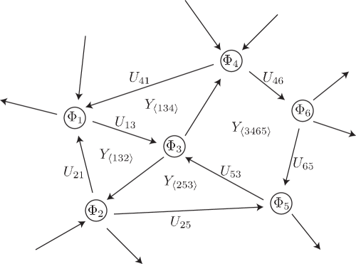
Figure 1: The structure of the generic lattice. We here show only the bosonic fields associated with each site, link and face.

We now introduce the BRST (supersymmetry) transformation for these variables by

$$\begin{array}[]{ll}Q_{s}\Phi_{x}=0,&\\ Q_{s}\bar{\Phi}_{x}=\eta_{x},&Q_{s}\eta_{x}=[\Phi_{x},\bar{\Phi}_{x}]\\ Q_{s}U_{xy}=i\lambda_{xy}U_{xy},&Q_{s}\lambda_{xy}=i(U_{xy}\Phi_{y}U_{xy}^{\dagger}-\Phi_{x}+\lambda_{xy}\lambda_{xy}),\\ Q_{s}Y_{f}=[\Phi_{f},\chi_{f}],&Q_{s}\chi_{f}=Y_{f},\end{array}$$ (4.1)

which are the lattice analog of (1.3) and (1.4). Here we denote the BRST charge by $Q_{s}$ to distinguish from the previous one. On all variables, the transformation satisfies $Q_{s}^{2}\cdot=i\delta_{\Phi}\cdot$ where $\delta_{\Phi}$ denotes an infinitesimal gauge transformation with the parameter $\Phi$. For later convenience, we define fermions on the links by $\Lambda_{xy}\equiv\lambda_{xy}U_{xy}$. Then the third line of the BRST transformation reduces to

$$Q_{s}U_{xy}=i\Lambda_{xy},\quad Q_{s}\Lambda_{xy}=i(U_{xy}\Phi_{y}-\Phi_{x}U_{xy})\,.$$ (4.2)

Using the above BRST transformation, the action can be written in a $Q_{s}$-exact form

$$S=\frac{1}{2g_{0}^{2}}Q_{s}\left[\sum_{x\in S}\alpha_{x}\Xi_{x}+\sum_{\langle xy\rangle\in L}\alpha_{\langle xy\rangle}\Xi_{\langle xy\rangle}+\sum_{f\in F}\alpha_{f}\Xi_{f}\right]\,,$$ (4.3)

with

$$\Xi_{x} \equiv\operatorname{Tr}\biggl{\{}\frac{1}{4}\eta_{x}[\Phi_{x},\bar{\Phi}_{x}]\biggr{\}},$$ (4.4)

$$\Xi_{\langle xy\rangle} \equiv\operatorname{Tr}\biggl{\{}-i\Lambda_{xy}(\bar{\Phi}_{y}U_{xy}^{\dagger}-U_{xy}^{\dagger}\bar{\Phi}_{x})\biggr{\}},$$ (4.5)

$$\Xi_{f} \equiv\operatorname{Tr}\biggl{\{}\chi_{f}(Y_{f}-i\beta_{f}\mu(U_{f}))\biggr{\}}\,,$$ (4.6)

where the coupling constants $\alpha_{x}$, $\alpha_{\langle xy\rangle}$, $\alpha_{f}$ and $\beta_{f}$ should be fixed in order to reproduce a correct continuum limit of the topological field theory [25]. However, surprisingly, the partition function and the vev of some physical observables are independent of them as we will see. The theory is constrained on $\mu(U_{f})=0$ after integrating out the auxiliary fields, where $\mu(U_{f})$ is a function of a plaquette variable $U_{f}$ defined by

$$U_{f}\equiv\prod_{i=0}^{n}U_{x_{i}x_{i+1}}\,,\quad(x_{n+1}=x_{0})$$ (4.7)

where $f=\langle x_{0}x_{1}\cdots x_{n}\rangle$ is the face surrounded by the links $\langle x_{0}x_{1}\rangle,\ldots,\langle x_{n}x_{0}\rangle$. The function $\mu(U_{f})$ is associated with the D-term constraint (moment map) in the continuum theory. In the lattice gage theory, we can choose $\mu(U_{f})$ so that $U_{f}=1$ is the unique solution of the vacuum equation $\mu(U_{f})=0$. For detail see Ref. [41]. After acting $Q_{s}$ in (4.3), we obtain the explicit form of the action

$$\begin{split}S&=\frac{1}{2g_{0}^{2}}\operatorname{Tr}\Biggr{[}\sum_{x\in S}\frac{\alpha_{x}}{4}[\Phi_{x},\bar{\Phi}_{x}]^{2}+\sum_{\langle xy\rangle\in L}\alpha_{\langle xy\rangle}|U_{xy}\Phi_{y}-\Phi_{x}U_{xy}|^{2}+\sum_{f\in F}\alpha_{f}Y_{f}(Y_{f}-i\beta_{f}\mu(U_{f}))\\ &\qquad\qquad\quad-\sum_{x\in S}\frac{\alpha_{x}}{4}\eta_{x}[\Phi_{x},\eta_{x}]\\ &\qquad\qquad\quad+\sum_{\langle xy\rangle\in L}i\alpha_{\langle xy\rangle}\Lambda_{xy}(\eta_{x}U_{xy}^{\dagger}-U^{\dagger}_{xy}\eta_{x}-\bar{\Phi}_{y}U_{xy}^{\dagger}\Lambda_{xy}U_{xy}^{\dagger}+U_{xy}^{\dagger}\Lambda_{xy}U_{xy}^{\dagger}\bar{\Phi}_{x})\\ &\qquad\qquad\quad+\sum_{f\in F}\alpha_{f}\left(-\chi_{f}[\Phi,_{f}\chi_{f}]+i\chi_{f}\beta_{f}Q_{s}\mu(U_{f})\right)\Biggr{]}\,.\end{split}$$ (4.8)

4.2 Localization and exact results

To proceed the localization argument, we first show the partition function is independent of the coupling constants; $g_{0}$, $\alpha_{x}$, $\alpha_{\langle xy\rangle}$, $\alpha_{f}$ and $\beta_{f}$. First of all, noting that we can always rescale pairs of the variables $(\bar{\Phi}_{x},\eta_{x})$ and $(Y_{f},\chi_{f})$ without changing the measure because of the supersymmetry. This means that the partition function is invariant under the change of the coupling constants

$$\begin{array}[]{lcl}\alpha_{x}\to c_{1}^{2}\alpha_{x},&&\alpha_{\langle xy\rangle}\to c_{1}\alpha_{\langle xy\rangle},\\ \alpha_{f}\to c_{2}^{2}\alpha_{f},&&\beta_{f}\to c_{2}\beta_{f},\end{array}$$ (4.9)

with constants $c_{1}$ and $c_{2}$. In addition, we can show that the partition function is completely independent of the couplings $\alpha_{x}$ and $\alpha_{f}$, since the action constructing from $\Xi_{x}$ and the first term of $\Xi_{f}$ is essentially Gaussian and there is no contribution from the moduli boundary. Combining them, we see that the partition function is independent of all of the coupling constants. The independence of the overall coupling $g_{0}$ is apparent since we can always include $g_{0}$ to the others.

Using the coupling independence, we choose all of coupling to be $\alpha_{x}=\alpha_{\langle xy\rangle}=\alpha_{f}=\beta_{f}=1$, except for the overall coupling $g_{0}$, in the following. Then the $Q_{s}$-exact action can be simply written as

$$S=\frac{1}{2g_{0}^{2}}Q_{s}\operatorname{Tr}\Big{[}\vec{{\cal F}}\cdot\overline{Q_{s}\vec{{\cal F}}}-i\sum_{f\in F}\chi_{f}\mu(U_{f})\Big{]}\,,$$ (4.10)

where we have introduced the sets of bosonic and fermionic fields $\vec{{\cal B}}=(\bar{\Phi}_{x},U_{xy},Y_{f})$ and $\vec{{\cal F}}=(\eta_{x},\Lambda_{xy},\chi_{f})$, respectively, and “ $\cdot$ ” denotes a suitable inner product with summation over corresponding variables associated with the lattice structure. Thus we can regard the supersymmetric lattice gauge theory as a supersymmetric Gaussian matrix model with a constraint by the moment maps $\mu(U_{f})=0$. Moreover, using the coupling independence of $g_{0}$, we find that the partition function and vev of physical observables are exactly evaluated at the 1-loop level, and the path integral is localized at the set of the BRST fixed point $Q\vec{\cal F}=0$ and the moment map constraint $\mu(U_{f})=0$.

In evaluating the partition function, we first fix the gauge by diagonalizing $\Phi_{x}$ as

$$\Phi_{x}=\operatorname{diag}(\phi_{x,1},\phi_{x,2},\ldots,\phi_{x,N}).$$ (4.11)

Note that this gauge breaks the gauge group from $\prod_{x\in S}U(N)$ to $\prod_{x\in S}U(1)^{N}$. The most nontrivial BRST fixed point condition is that for the link fermions,

$$U_{xy}\Phi_{y}-\Phi_{x}U_{xy}=0\quad\text{for }{}^{\forall}\langle xy\rangle\in L,$$ (4.12)

which can be solved by

$$U_{xy}=\Gamma_{xy}\in\mathfrak{S}_{N},$$ (4.13)

where $\mathfrak{S}_{N}$ is the permutation (Weyl) subgroup in $U(N)$, since $\Phi_{x}$ is diagonal. Thus we find that the diagonal elements of $\Phi_{x}$ between neighbor nodes are related with each other by the permutations

$$\Phi_{y}=\Gamma_{xy}^{\dagger}\Phi_{x}\Gamma_{xy}.$$ (4.14)

This means that all the eigenvalues of $\Phi_{x}$ are expressed by permutations of a representative eigenvalue at some point. If we denote the representative eigenvalue by $\phi_{i}$, the other eigenvalues are determined by a permutation of it, namely

$$\phi_{x,i}=\phi_{\sigma_{x}(i)},$$ (4.15)

where $\sigma_{x}(i)\in\mathfrak{S}_{N}$ and we have assumed that all the sites are connected.

In addition, the moment map constraint $\mu(U_{f})=0$ requires

$$\left.U_{f}\right|_{U_{xy}=\Gamma_{xy}}=1,$$ (4.16)

which is also a consistency condition of the permutations around any face. So we can choose sets of the possible permutations which satisfy the constraint by each face $f$. Thus the eigenvalue at each point is also determined by the chain of the possible permutations from the representative point.

In evaluating the partition function in the saddle point approximation, we have to compute the 1-loop determinant (Jacobian of the Gaussian integrals) around the fixed points, which is obtained as the determinant of the super Hessian matrix (see [42, 43] and Appendix A)

(1-loop det) $$=\sqrt{\frac{\operatorname{Det}^{\prime}\frac{\delta Q_{s}\vec{{\cal B}}}{\delta\vec{{\cal F}}}}{\operatorname{Det}^{\prime}\frac{\delta Q_{s}\vec{{\cal F}}}{\delta\vec{{\cal B}}}}}\,,$$ (4.17)

where each determinant is taken only over non-zero modes (non-zero eigenvalues). Here we have to carefully remove the zero modes in the determinant to avoid zeros or divergences. Evaluating the above 1-loop determinant of our model in the diagonal gage, we find

$$\begin{split}\text{(1-loop det)}&=\sqrt{\frac{\frac{\delta Q_{s}\eta_{x}}{\delta\bar{\Phi}_{x}}}{\frac{\delta Q_{s}\eta_{x}}{\delta\bar{\Phi}_{x}}\frac{\delta Q_{s}U_{xy}}{\delta\Lambda_{xy}}}}\\ &=\sqrt{\frac{\prod_{f\in F}\prod_{\sigma_{f}(i)\neq\sigma_{f}(j)}(\phi_{\sigma_{f}(i)}-\phi_{\sigma_{f}(j)})}{\prod_{x\in S}\prod_{\sigma_{x}(i)\neq\sigma_{x}(j)}(\phi_{\sigma_{x}(i)}-\phi_{\sigma_{x}(j)})\prod_{\langle xy\rangle\in L}\prod_{\sigma_{x}(i)\neq\sigma_{y}(j)}(\phi_{\sigma_{x}(i)}-\phi_{\sigma_{y}(j)})}},\end{split}$$ (4.18)

where $\phi_{\sigma_{f}(i)}$ stands for an eigenvalue at an arbitrary point on the face $f$.

In addition to the above 1-loop determinant, we also need the Vandermonde determinant at each point $\prod_{x\in S}\prod_{\sigma_{x}(i)\neq\sigma_{x}(j)}(\phi_{\sigma_{x}(i)}-\phi_{\sigma_{x}(j)})$, which appears in the integration of the gauge fixing ghosts. Combining the 1-loop determinant with the Vandermonde determinant, we obtain the partition function as an integration over the representative eigenvalue and a summation over the possible permutations (fixed points)

$$\begin{split}Z&=\sum_{\sigma_{x}:\text{possible permutations}}\int\prod_{i=1}^{N}\frac{d\phi_{i}}{2\pi i}\\ &\qquad\times\sqrt{\frac{\prod_{x\in S}\prod_{\sigma_{x}(i)\neq\sigma_{x}(j)}(\phi_{\sigma_{x}(i)}-\phi_{\sigma_{x}(j)})\prod_{f\in F}\prod_{\sigma_{f}(i)\neq\sigma_{f}(j)}(\phi_{\sigma_{f}(i)}-\phi_{\sigma_{f}(j)})}{\prod_{\langle xy\rangle\in L}\prod_{\sigma_{x}(i)\neq\sigma_{y}(j)}(\phi_{\sigma_{x}(i)}-\phi_{\sigma_{y}(j)})}}.\end{split}$$ (4.19)

Using the fact that the difference product of the eigenvalues in the integrand is invariant under the permutations and the contributions to the measure from each permutation are identical, we finally obtain a simple expression of the partition function

$$Z={\cal C}\int\prod_{i=1}^{N}\frac{d\phi_{i}}{2\pi i}\prod_{i<j}(\phi_{i}-\phi_{j})^{n_{S}-n_{L}+n_{F}},$$ (4.20)

where $n_{S}$, $n_{L}$ and $n_{F}$ are the numbers of sites, links and faces, respectively, and ${\cal C}$ is the total number of the possible permutations. We here would like to emphasize that the original path integral of the lattice gauge theory reduces to an integral over only $N$ eigenvalues at the representative point, thanks to the localization.

Here the combination $\chi\equiv n_{S}-n_{L}+n_{F}$ is nothing but the Euler characteristic which depends only on the topology of the two-dimensional surface. It is remarkable that the final result of the partition function (4.20) is the same as the partition function of (topologically twisted) ${\cal N}=(2,2)$ supersymmetric Yang-Mills theory on the smooth Riemann surface (continuum space-time) [1, 2, 3]. The integral (4.20) of the partition function diverges in general for $\chi\geq 0$. This fact reflects the existence of the flat direction of the supersymmetric theory. In order to regularize the divergence from the flat direction, we need to turn on a potential without spoiling the localization argument. This is done by introducing physical observables (BRST closed operators) as we will discuss in the next subsection.

Before going to the next subsection, we mention that there is an alternative way to take into account the zero-modes at the fixed points by using a residue integral over eigenvalues of $\Phi_{x}$’s. To see this, let us go back to the original expression of the partition function (4.10) in the diagonal gauge (4.11). Since we can use the formula for the 1-loop determinant (4.17) before localizing the path integral over $\Phi_{x}$, we obtain

$$Z=\int\prod_{x\in S}\prod_{i=1}^{N}\frac{d\phi_{x,i}}{2\pi i}\frac{\prod_{x\in S}\prod_{i<j}(\phi_{x,i}-\phi_{x,j})\prod_{f\in F}\prod_{i<j}(\phi_{f,i}-\phi_{f,j})}{\prod_{\langle xy\rangle\in L}\prod_{i\leq j}(\phi_{x,i}-\phi_{y,j})}\,.$$ (4.21)

To integrate the diagonal elements of $\Phi_{x}$, we need to choose suitable contours for each $\phi_{x,i}$, which corresponds to the gauge fixing of the residual $U(1)$’s and moment map constraints [44]. By choosing the contours and picking up the poles in the integral (4.21), we obtain an integral results as a residue integral. The poles of the integrand exactly correspond to the BRST fixed point equation (4.12), which leads the same result (4.20).

4.3 Observables and Ward-Takahashi identities

Let us next consider observables in this theory. In the context of topological field theory, such operators that are in $Q_{s}$-cohomology are called physical operators. In general, the physical observable has a non-trivial vev, while that of the $Q_{s}$-exact operator vanishes. An important physical observable in our system is the sKM action introduced in the previous section. Indeed, the sKM action (3.6) satisfies

$$Q_{s}S_{\rm sKM}=0,$$ (4.22)

but it is not $Q_{s}$-exact. The potential part of the sKM action, which is a function of $\Phi_{x}$ only, is apparently $Q_{s}$-closed because of the BRST transformation $Q_{s}\Phi_{x}=0$. Although the $Q_{s}$-closedness of the residual part of the sKM action is not so much clear at the first sight, we can see it by the identity,

$$Q_{s}\left[-i\operatorname{Tr}\Lambda_{xy}\Phi_{y}U_{xy}^{\dagger}\right]=-\operatorname{Tr}\left\{\Phi_{x}U_{xy}\Phi_{y}U_{xy}^{\dagger}-\frac{1}{2}\lambda_{xy}[U_{xy}\Phi_{y}U_{xy}^{\dagger},\lambda_{xy}]\right\}+\operatorname{Tr}\Phi_{x}^{2},$$ (4.23)

which includes a part of the sKM action. Noting that $Q_{s}^{2}=0$ on the gauge invariant operator and trivially $Q_{s}\operatorname{Tr}\Phi_{x}^{2}=0$, we immediately conclude (4.22).

In addition, using the fact that the vev of the $Q_{s}$-exact operator vanishes, we find a Ward-Takahashi identity in the supersymmetric lattice gauge theory

$$\left\langle S_{\rm sKM}\right\rangle=-\left\langle\sum_{\langle xy\rangle\in L}\operatorname{Tr}\Phi_{x}^{2}\right\rangle+\left\langle\sum_{x\in S}\operatorname{Tr}V(\Phi_{x})\right\rangle$$ (4.24)

As we will see, we can explicitly check this identity form the localization point of view.

The sKM action is a “good” observable in the supersymmetric lattice gauge theory in the above sense. So we can exactly evaluate the vev of the sKM action. In particular, the exponent of the sKM action induces potentials of the scalar field $\Phi_{x}$

$$\left\langle e^{\gamma S_{\rm sKM}}\right\rangle=\left\langle e^{\gamma\operatorname{Tr}\left\{-\sum_{\langle xy\rangle\in L}\operatorname{Tr}\Phi_{x}^{2}+\sum_{x\in S}\operatorname{Tr}V(\Phi_{x})\right\}}\right\rangle,$$ (4.25)

where $\gamma$ is an arbitrary parameter and we have flipped the sign of the coupling constant in front of the sKM action to utilize for a regulator of the flat directions of the supersymmetric lattice gauge theory.

Repeating the localization argument, we can evaluate the vev of the sKM model action exactly by

$$\left\langle e^{\gamma S_{\rm sKM}}\right\rangle=\int\prod_{x\in S}\prod_{i=1}^{N}\frac{d\phi_{x,i}}{2\pi i}\frac{\prod_{x\in S}\prod_{i<j}(\phi_{x,i}-\phi_{x,j})\prod_{f\in F}\prod_{i<j}(\phi_{f,i}-\phi_{f,j})}{\prod_{\langle xy\rangle\in L}\prod_{i\leq j}(\phi_{x,i}-\phi_{y,j})}e^{\gamma S_{\rm sKM}}.$$ (4.26)

The fixed points (poles) are classified by the permutation group again. For the vev of the sKM model, we see

$$\left\langle S_{\rm sKM}\right\rangle=-\sum_{\langle xy\rangle\in L}\sum_{i=1}^{N}\phi_{x,i}^{2}+\sum_{x\in S}\sum_{i=1}^{N}\phi_{x,i}^{2}=(n_{S}-n_{L})\sum_{i=1}^{N}\phi_{i}^{2},$$ (4.27)

at the each fixed point. The measure gives the same contribution $\prod_{i<j}(\phi_{i}-\phi_{j})^{\chi}$ as the partition function. We then obtain

$$\left\langle e^{\gamma S_{\rm sKM}}\right\rangle={\cal C}\int\prod_{i=1}^{N}d\phi_{i}\prod_{i<j}(\phi_{i}-\phi_{j})^{\chi}e^{\gamma(n_{S}-n_{L})\sum_{i=1}^{N}\phi_{i}^{2}},$$ (4.28)

where the number of the possible permutations (fixed points) ${\cal C}$ appears again. Noting that $n_{S}-n_{L}=\chi-n_{F}$ by using the definition of the Euler characteristic, the coefficient of the potential $\gamma(n_{S}-n_{L})$ becomes negative for the large $n_{F}$, since $\chi$ is constant for the same Riemann surface. So the vev (4.28) is regularized in the sense of the Gaussian integral, in comparison with the partition function itself.

Finally, we would like to discuss the continuum limit of (4.28). Let $a^{2}$ denote the average area of the faces. As discussed in [25], the continuum limit is defined by $a\to 0$ and $n_{F}\to\infty$ with fixing the combination $a^{2}n_{F}$ to the the total area of the Riemann surface ${\cal A}$. The scalar field $\Phi_{x}$ in the lattice theory is related with the continuum field $\Phi(x)$ such that $\Phi_{x}=a\Phi(x)$. If we use the discretization of the Riemann surface with the same Euler characteristic (genus), we find

$$\gamma a^{2}(n_{S}-n_{L})\sum_{i=1}^{N}\tilde{\phi}_{i}^{2}=\gamma a^{2}(\chi-n_{F})\sum_{i=1}^{N}\tilde{\phi}_{i}^{2}\ \to\ -\gamma{\cal A}\sum_{i=1}^{N}\tilde{\phi}_{i}^{2},$$ (4.29)

where $\tilde{\phi}_{i}$’s are eigenvalues of the continuum field. Then we obtain, in the continuum limit,

$$\left\langle e^{\gamma S_{\rm sKM}}\right\rangle=\tilde{{\cal C}}\int\prod_{i=1}^{N}d\tilde{\phi}_{i}\prod_{i<j}(\tilde{\phi}_{i}-\tilde{\phi}_{j})^{\chi}e^{-\gamma{\cal A}\sum_{i=1}^{N}\tilde{\phi}_{i}^{2}},$$ (4.30)

where $\tilde{{\cal C}}\equiv{\cal C}a^{N+\chi N(N-1)/2}$ is also fixed. This expression is essentially the same as the partition function of two-dimensional YM theory appeared in (1.7), except for the summation over the flux configurations. Thus we successfully reproduce the perturbative partition function of the continuous two-dimensional YM theory from the continuum limit of the discretized theory.

5 Conclusion and Discussion

In this paper, we discussed the localization mechanism in the various unitary matrix models, which includes the two-dimensional supersymmetric gauge theory on a generic discretized Riemann surface (generalized Sugino model). The integrability of the unitary matrix models based on the localization still holds as well as the lower dimensional continuous gauge theories.

We also find that the integral formula of the partition function of the two-dimensional supersymmetric lattice gauge theory is identical with the continuum one. It depends only on the Euler characteristic and size of the system (topology and area of the Riemann surface). This fact may come from the specialty of the two-dimensional YM theory, which is almost topological, namely invariant under the area preserving diffeomorphism. The two-dimensional discretized YM theory inherits this topological property, and so is solved exactly. The potential gain of this study is simplification of numerical analysis of the supersymmetric lattice models. While several numerical studies of the Sugino models have been in progress [35, 36, 37, 38, 39, 40, 41], our reduced path integral would simplify and accelerate the numerical calculations.

This work for the first time evaluates completely the lattice path integrals by the localization technique, which can be seen as the multi-matrix extension of the HCIZ integral based on the equivariant cohomology. In this sense, our study connects the well-defined equivariant localization to the empirical supersymmetric localization, which backs up validity of the localization technique in the field theory.

We here frankly refer to an insufficient point of this work: We have discussed the partition function itself and some vevs of the physical observables without summing up the non-perturbative flux configurations, since we do not have an operator depending on the flux. However, as we mentioned in the introduction, the continuum theory has a specific operator which depends on the fluxes and we obtain the partition function of the bosonic (non-supersymmetric) two-dimensional YM theory as the vev of the operator. It is an interesting problem to find the corresponding operator, which depends on the non-trivial fluxes and reproduces the partition function of the bosonic lattice gauge theory.

We finally comment on the relation to the quiver gauge theory. We have considered the multi unitary matrix model on the lattice, while we can also regard it as a quiver (unitary) matrix model associated with the lattice structure: We identify sites, links and faces with nodes, arrows and loops (superpotentials) in the quiver matrix model, respectively. It is known that the quiver theories, including the quiver matrix models and quiver quantum mechanics, are important in the context of the superstring (supergravity) theory or $M$-theory. (See e.g. [45, 44].) We expect that our exact result and simulation techniques in the supersymmetric lattice gauge theories also shed light on the superstring and $M$-theory.

Appendix A Derivation of the 1-loop Determinants

Here we derive the 1-loop determinant for a general matrix model induced by the supersymmetric Yang-Mills theory. Let us first consider a set of the bosonic matrix variables ${\cal B}^{I}$ and the fermionic matrix variables ${\cal F}^{I}$, except for $\Phi$ which satisfies $Q\Phi=0$. We assume that $\frac{\delta Q{\cal F}^{I}}{\delta{\cal F}^{J}}=\frac{\delta Q{\cal B}^{I}}{\delta{\cal B}^{J}}=0$.

The $Q$-exact action is

$$\begin{split}S&=tQ\operatorname{Tr}\bigg{[}g_{IJ}{\cal F}^{I}\overline{Q{\cal F}^{J}}\bigg{]}\\ &=t\operatorname{Tr}\bigg{[}||Q\vec{{\cal F}}||^{2}-{\cal F}^{I}Q(g_{IJ}\overline{Q{\cal F}^{J}})\bigg{]},\end{split}$$ (A.1)

where the metric $g_{IJ}$ is a scalar function of $\vec{{\cal B}}$ only, and $||\cdots||^{2}$ denotes a suitable norm of the vector of the fields. We can show that a partition function with respect to the above action is independent of the coupling $t$, and the path integral localizes at the fixed point equation $Q{\cal F}^{I}=Q{\cal B}^{I}=0$.

If we denote the solution of the fixed point equation by ${\cal B}_{0}^{I}$ and ${\cal F}_{0}^{I}$, then we can expand the fields around the fixed point by

$$\begin{split}{\cal B}^{I}&={\cal B}_{0}^{I}+\frac{1}{\sqrt{t}}\tilde{{\cal B}}^{I},\\ {\cal F}^{I}&={\cal F}_{0}^{I}+\frac{1}{\sqrt{t}}\tilde{{\cal F}}^{I}.\\ \end{split}$$ (A.2)

Substituting the expansion (A.2), up to the quadratic order, the action becomes,

$$S=\operatorname{Tr}\bigg{[}G_{IJ}\tilde{{\cal B}}^{I}\tilde{{\cal B}}^{J}-\Omega_{IJ}\tilde{{\cal F}}^{I}\tilde{{\cal F}}^{J}\bigg{]}+{\cal O}(1/\sqrt{t}),$$ (A.3)

where

$$\begin{split}G_{IJ}&=\left.\frac{\delta^{2}}{\delta{\cal B}^{I}\delta{\cal B}^{J}}||Q\vec{{\cal F}}||^{2}\right|_{\vec{{\cal B}}=\vec{{\cal B}}_{0}},\\ \Omega_{IJ}&=\frac{1}{2}\left.\left(\frac{\delta}{\delta{\cal F}^{I}}Q(g_{JK}\overline{Q{\cal F}^{K}})-\frac{\delta}{\delta{\cal F}^{J}}Q(g_{IK}\overline{Q{\cal F}^{K}})\right)\right|_{\vec{{\cal F}}=\vec{{\cal F}}_{0}}\end{split}$$ (A.4)

The quadratic action (A.3) itself should be $Q$-closed (supersymmetric) since it is independent of the coupling $t$. So we find

$$G_{IJ}(Q\tilde{{\cal B}}^{I})\tilde{{\cal B}}^{J}=\Omega_{IJ}(Q\tilde{{\cal F}}^{I})\tilde{{\cal F}}^{J},$$ (A.5)

where we have used the fact that $QG_{IJ}=Q\Omega_{IJ}=0$ since $G_{IJ}$ and $\Omega_{IJ}$ are defined at the fixed point value and behave as constants.

Let us next consider an expansion of $Q{\cal F}^{I}$ and $Q{\cal B}^{I}$ around the fixed point

$$\begin{split}Q{\cal F}^{I}&=\left.Q{\cal F}^{I}\right|_{\vec{{\cal B}}=\vec{{\cal B}}_{0}}+\frac{1}{\sqrt{t}}\left.\frac{\delta Q{\cal F}^{I}}{\delta{\cal B}^{J}}\right|_{\vec{{\cal B}}=\vec{{\cal B}}_{0}}\tilde{{\cal B}}^{J},\\ Q{\cal B}^{I}&=\left.Q{\cal B}^{I}\right|_{\vec{{\cal F}}=\vec{{\cal F}}_{0}}+\frac{1}{\sqrt{t}}\left.\frac{\delta Q{\cal B}^{I}}{\delta{\cal F}^{J}}\right|_{\vec{{\cal F}}=\vec{{\cal F}}_{0}}\tilde{{\cal F}}^{J}\end{split}$$ (A.6)

while, from (A.2), we see

$$\begin{split}Q{\cal F}^{I}&=Q{\cal F}_{0}^{I}+\frac{1}{\sqrt{t}}Q\tilde{{\cal F}}^{I},\\ Q{\cal B}^{I}&=Q{\cal B}_{0}^{I}+\frac{1}{\sqrt{t}}Q\tilde{{\cal B}}^{I}.\end{split}$$ (A.7)

Then we have

$$\begin{split}Q\tilde{{\cal F}}^{I}&=\left.\frac{\delta Q{\cal F}^{I}}{\delta{\cal B}^{J}}\right|_{\vec{{\cal B}}=\vec{{\cal B}}_{0}}\tilde{{\cal B}}^{J},\\ Q\tilde{{\cal B}}^{I}&=\left.\frac{\delta Q{\cal B}^{I}}{\delta{\cal F}^{J}}\right|_{\vec{{\cal F}}=\vec{{\cal F}}_{0}}\tilde{{\cal F}}^{J}\end{split}$$ (A.8)

Substituting (A.8) into (A.5), we find a relation

$$G_{IJ}\left.\frac{\delta Q{\cal B}^{I}}{\delta{\cal F}^{K}}\right|_{\vec{{\cal F}}=\vec{{\cal F}}_{0}}=\Omega_{IK}\left.\frac{\delta Q{\cal F}^{I}}{\delta{\cal B}^{J}}\right|_{\vec{{\cal B}}=\vec{{\cal B}}_{0}}$$ (A.9)

Thus we obtain a relation between determinants of $G_{IJ}$ and $\Omega_{IJ}$

$$\frac{\operatorname{Det}\Omega_{IJ}}{\operatorname{Det}G_{IJ}}=\frac{\operatorname{Det}\frac{\delta Q{\cal B}^{I}}{\delta{\cal F}^{J}}}{\operatorname{Det}\frac{\delta Q{\cal F}^{I}}{\delta{\cal B}^{J}}},$$ (A.10)

at the fixed points.

Using the above relations, we can evaluate the partition function by

$$\begin{split}Z&=\int\prod_{I}{\cal D}{\cal B}^{I}{\cal D}{\cal F}^{I}\,e^{-S(\vec{{\cal B}},\vec{{\cal F}})}\\ &=\sum_{\text{fixed points}}\int\prod_{I}{\cal D}\tilde{{\cal B}}^{I}{\cal D}\tilde{{\cal F}}^{I}\,e^{-\operatorname{Tr}\left[G_{IJ}\tilde{{\cal B}}^{I}\tilde{{\cal B}}^{J}-\Omega_{IJ}\tilde{{\cal F}}^{I}\tilde{{\cal F}}^{J}\right]}\\ &=\sum_{\text{fixed points}}\sqrt{\frac{\operatorname{Det}\Omega_{IJ}}{\operatorname{Det}G_{IJ}}}\\ &=\sum_{\text{fixed points}}\sqrt{\frac{\operatorname{Det}\frac{\delta Q{\cal B}^{I}}{\delta{\cal F}^{J}}}{\operatorname{Det}\frac{\delta Q{\cal F}^{I}}{\delta{\cal B}^{J}}}}.\end{split}$$ (A.11)

This is a formula of the 1-loop determinant.

References

- [1] E. Witten, Two-dimensional gauge theories revisited, J.Geom.Phys. 9 (1992) 303–368 [hep-th/9204083].
- [2] M. Blau and G. Thompson, “Lectures on 2-d gauge theories: Topological aspects and path integral techniques,” hep-th/9310144.
- [3] M. Blau and G. Thompson, “Localization and diagonalization: A review of functional integral techniques for low dimensional gauge theories and topological field theories,” J. Math. Phys. 36, 2192 (1995) [hep-th/9501075].
- [4] C. Beasley and E. Witten, J. Diff. Geom. 70, 183 (2005) [hep-th/0503126].
- [5] A. Kapustin, B. Willett and I. Yaakov, JHEP 1003, 089 (2010) [arXiv:0909.4559 [hep-th]].
- [6] E. Witten, Topological Quantum Field Theory, Commun. Math. Phys. 117 (1988) 353.
- [7] E. Witten, Introduction to cohomological field theories, Int. J. Mod. Phys. A6 (1991) 2775–2792.
- [8] V. Pestun, Localization of gauge theory on a four-sphere and supersymmetric Wilson loops, Commun.Math.Phys. 313 (2012) 71–129 [0712.2824].
- [9] J. J. Duistermaat and G. J. Heckman, “On the Variation in the cohomology of the symplectic form of the reduced phase space,” Invent. Math. 69, 259 (1982).
- [10] T. Karki and A. J. Niemi, “On the Duistermaat-Heckman formula and integrable models,” hep-th/9402041.
- [11] A. A. Migdal, “Recursion Equations in Gauge Theories,” Sov. Phys. JETP 42, 413 (1975) [Zh. Eksp. Teor. Fiz. 69, 810 (1975)].
- [12] D. B. Kaplan, E. Katz and M. Unsal, Supersymmetry on a spatial lattice, JHEP 05 (2003) 037 [hep-lat/0206019].
- [13] A. G. Cohen, D. B. Kaplan, E. Katz and M. Unsal, Supersymmetry on a Euclidean spacetime lattice. I: A target theory with four supercharges, JHEP 08 (2003) 024 [hep-lat/0302017].
- [14] A. G. Cohen, D. B. Kaplan, E. Katz and M. Unsal, Supersymmetry on a Euclidean spacetime lattice. II: Target theories with eight supercharges, JHEP 12 (2003) 031 [hep-lat/0307012].
- [15] D. B. Kaplan and M. Unsal, A Euclidean lattice construction of supersymmetric Yang- Mills theories with sixteen supercharges, JHEP 09 (2005) 042 [hep-lat/0503039].
- [16] F. Sugino, A lattice formulation of super Yang-Mills theories with exact supersymmetry, JHEP 01 (2004) 015 [hep-lat/0311021].
- [17] F. Sugino, Super Yang-Mills theories on the two-dimensional lattice with exact supersymmetry, JHEP 03 (2004) 067 [hep-lat/0401017].
- [18] F. Sugino, Various super Yang-Mills theories with exact supersymmetry on the lattice, JHEP 01 (2005) 016 [hep-lat/0410035].
- [19] F. Sugino, Two-dimensional compact N = (2,2) lattice super Yang-Mills theory with exact supersymmetry, Phys. Lett. B635 (2006) 218–224 [hep-lat/0601024].
- [20] F. Sugino, Lattice Formulation of Two-Dimensional N=(2,2) SQCD with Exact Supersymmetry, Nucl.Phys. B808 (2009) 292–325 [0807.2683].
- [21] J. Giedt and E. Poppitz, JHEP 0409, 029 (2004) [hep-th/0407135].
- [22] N. Sakai and M. Sakamoto, Nucl. Phys. B 229, 173 (1983).
- [23] Y. Kikukawa and Y. Nakayama, Phys. Rev. D 66, 094508 (2002) [hep-lat/0207013].
- [24] K. Ohta and T. Takimi, Prog. Theor. Phys. 117, 317 (2007) [hep-lat/0611011]; PoS LAT 2007, 279 (2007) [arXiv:0710.0438 [hep-lat]].
- [25] S. Matsuura, T. Misumi and K. Ohta, “Topologically Twisted Supersymmetric Yang-Mills Theory on Arbitrary Discretized Riemann Surface,” arXiv:1408.6998 [hep-lat].
- [26] V. A. Kazakov and A. A. Migdal, “Induced QCD at large N,” Nucl. Phys. B 397, 214 (1993) [hep-th/9206015].
- [27] I. I. Kogan, A. Morozov, G. W. Semenoff and N. Weiss, “Area law and continuum limit in ’induced QCD’,” Nucl. Phys. B 395, 547 (1993) [hep-th/9208012].
- [28] Harish-Chandra, Amer.J.Math, 79, 87-120, (1957).
- [29] C. Itzykson and J. B. Zuber, “The Planar Approximation. 2.,” J. Math. Phys. 21, 411 (1980).
- [30] R. J. Szabo, “Equivariant localization of path integrals,” hep-th/9608068.
- [31] R. J. Szabo, “Equivariant Cohomology and Localization of Path Integrals,” Lect. Notes Phys. M 63, 1 (2000).
- [32] A. A. Kirillov, “Elements of the theory of representations”, Representations of groups, Springer-Verlag Berlin, (1976).
- [33] B. Kostant, “Orbits and Quantization Theory”, Congrés intern.Math., 395-405, (1970).
- [34] J. M. Souriau, “Structure of Dynamical Systems: A Symplectic View of Physics”, Progress in Mathematics, Birkhäuser Boston, (1997).
- [35] H. Suzuki, Two-dimensional super Yang-Mills theory on computer, JHEP 09 (2007) 052 [0706.1392].
- [36] I. Kanamori, H. Suzuki and F. Sugino, Euclidean lattice simulation for the dynamical supersymmetry breaking, 0711.2099.
- [37] I. Kanamori, F. Sugino and H. Suzuki, Observing dynamical supersymmetry breaking with euclidean lattice simulations, 0711.2132.
- [38] I. Kanamori and H. Suzuki, Restoration of supersymmetry on the lattice: Two-dimensional N = (2,2) supersymmetric Yang-Mills theory, Nucl.Phys. B811 (2009) 420–437 [0809.2856].
- [39] M. Hanada and I. Kanamori, Lattice study of two-dimensional N=(2,2) super Yang-Mills at large-N, Phys.Rev. D80 (2009) 065014 [0907.4966].
- [40] M. Hanada, S. Matsuura and F. Sugino, Non-perturbative construction of 2D and 4D supersymmetric Yang-Mills theories with 8 supercharges, Nucl.Phys. B857 (2012) 335–361 [1109.6807].
- [41] S. Matsuura and F. Sugino, Lattice formulation for 2d = (2, 2), (4, 4) super Yang-Mills theories without admissibility conditions, JHEP 1404 (2014) 088 [1402.0952].
- [42] K. Ohta and Y. Yoshida, Phys. Rev. D 86, 105018 (2012) [arXiv:1205.0046 [hep-th]].
- [43] K. Ohta, N. Sakai and Y. Yoshida, PTEP 2013, no. 7, 073B03 (2013).
- [44] K. Ohta and Y. Sasai, “Exact Results in Quiver Quantum Mechanics and BPS Bound State Counting,” arXiv:1408.0582 [hep-th].
- [45] F. Denef, “Quantum quivers and Hall / hole halos,” JHEP 0210, 023 (2002) [hep-th/0206072].