The generic fixed point model for pseudo-spin-$\frac{1}{2}$ quantum dots in nonequilibrium: Spin-valve systems with compensating spin polarizations

Abstract

We study a pseudo-spin-$\frac{1}{2}$ quantum dot in the cotunneling regime close to the particle-hole symmetric point. For a generic tunneling matrix we find a generic fixed point with interesting nonequilibrium properties, characterized by effective reservoirs with compensating spin orientation vectors weighted by the polarizations and the tunneling rates. At large bias voltage we study the magnetic field dependence of the dot magnetization and the current. The fixed point can be clearly identified by analyzing the magnetization of the dot. We characterize in detail the universal properties for the case of two reservoirs.

Nonequilibrium properties of strongly interacting quantum dots have gained an enormous interest in the last decades. Quantum dots are experimentally controllable systems useful for a variety of applications in nanoelectronics, spintronics and quantum information processing review_qi . They are of fundamental interest in the field of open quantum systems in nonequilibrium with interesting quantum many-body properties and coherent phenomena at low temperatures andergassen_etal . Of particular interest are spin-dependent phenomena where the quantum dot is tuned to the Coulomb blockade regime. In the case of a singly-occupied dot the spin can fluctuate between two values leading to a realization of the isotropic spin-$\frac{1}{2}$ antiferromagnetic Kondo model. A hallmark was the prediction and observation of universal conductance for this model kondo_theo ; kondo_exp . The equilibrium properties of the Kondo model have been studied extensively costi_etal_94 ; glazman_pustilnik_05 and, most recently, by using renormalization group (RG) methods in nonequilibrium, also the properties at finite bias voltage and the time dynamics have been analyzed in weak rosch_etal ; kehrein_etal ; schoeller_epj09 ; hs_reininghaus_prb09 ; pletyukhov_etal_prl10 and strong coupling frg_noneq ; strong_coupling_RTRG ; smirnov_grifoni_03 and compared to experiments strong_coupling_exp .

The isotropic Kondo model with unpolarized leads is only a special case out of the whole class of quantum dot models where a single particle on the dot can fluctuate between two different quantum numbers (which we call a pseudo-spin-$\frac{1}{2}$ quantum dot in the following). Besides the case of ferromagnetic leads with arbitrary spin orientations the two quantum numbers can also label two different orbitals or can arise from a mixture of spin and orbital degrees of freedom in the presence of spin-orbit interaction in the leads or on the dot, leading to non-spin-conserving tunneling matrices. In equilibrium (or the linear response regime), it has been found for several cases that exchange fields are generated but if those are canceled by external ones the universality properties of the Kondo model are re-established. This has been confirmed by numerical renormalization group (NRG) calculations for ferromagnetic leads with parallel or antiparallel orientations koenig_nrg and for quantum dots with orbital degrees of freedom or Aharonov-Bohm geometries boese_etal . In Ref. kashcheyevs_etal_prb07, a mapping between these different models and an analytical understanding in terms of the anisotropic Kondo model has been established. Concerning nonequilibrium transport previous studies have focused on exchange fields generated by ferromagnetic leads koenig_etal , spin-orbit interaction paaske_etal_prb10 or orbital fluctuations boese_etal . A systematic nonequilibrium RG study of a pseudo-spin-$\frac{1}{2}$ quantum dot with spin-orbit interaction in the cotunneling regime has been performed in Ref. pletyukhov_schuricht_prb11, , where a Dzyaloshinskii-Moriya (DM) interaction together with exchange fields proportional to the bias voltage have been identified. For special orientations of the DM-vectors interesting asymmetries in resonant transport where reported when a magnetic field of the order of the bias voltage is applied.

Figure 1: (Color online) Sketch of the effective model of two ferromagnetic leads $\alpha=L,R$ coupled to a pseudo-spin-$\frac{1}{2}$ quantum dot via spin-conserving tunneling rates $\Gamma_{L,R}=x_{L,R}\Gamma$. $\mu_{L,R}=\pm V/2$ denote the chemical potentials of the leads with spin axis $\hat{\vec{d}}_{L,R}$ and spin polarization $p_{L,R}$. $h$ denotes the Zeeman splitting of the dot levels including exchange fields.

All previous references treated special cases of pseudo-spin-$\frac{1}{2}$ quantum dots without aiming at finding generic features common to all these systems, irrespective of the complexity of the geometry, the special interactions and the polarizations of the reservoirs. The purpose of this letter is to establish such features especially in the nonequilibrium regime. Thereby, we will first use a mapping to a pseudo-spin-$\frac{1}{2}$ quantum dot coupled to effective ferromagnetic leads as depicted in Fig. 1, similiar to Refs. koenig_etal ; kashcheyevs_etal_prb07 . Based on this model, we will show that in the Coulomb blockade regime close to the particle-hole symmetric point a fixed point model can be identified where the average of the unit vectors of the spin orientations $\hat{\vec{d}}_{\alpha}$ weighted by the polarizations $p_{\alpha}$ and the tunneling rates $\Gamma_{\alpha}$ compensate each other ($\alpha$ is the reservoir index)

$$\vec{d}=\sum_{\alpha}\vec{d}_{\alpha}=0\quad,\quad\vec{d}_{\alpha}=x_{\alpha}p_{\alpha}\hat{\vec{d}}_{\alpha}\quad,\quad x_{\alpha}=\frac{\Gamma_{\alpha}}{\Gamma}\quad,$$ (1)

with $\Gamma=\sum_{\alpha}\Gamma_{\alpha}$. This explains why the Kondo effect appears generically in the equilibrium case where all reservoirs can be taken together and (1) leads to a vanishing spin polarization, in agreement with Rfs. koenig_nrg, ; boese_etal, ; kashcheyevs_etal_prb07, . However, what has been overlooked so far is that the fixed point model is generically not the one of the Kondo model with one unpolarized lead but rather a spin-$\frac{1}{2}$ coupled to several leads with different spin vectors $\vec{d}_{\alpha}$. This is particularly important for the nonequilibrium case where the reservoirs cannot be taken together. Thus, an interesting fixed point emerges which, in the equilibrium case, leads to the usual Kondo physics, whereas, in the nonequilibrium regime, shows essentially different universal behavior compared to the Kondo model. We will characterize the universal features by calculating the magnetic field dependence of the dot magnetization and the charge current at zero temperature and large chemical potentials $\mu_{\alpha}$ compared to the Kondo temperature $T_{K}$ at and away from the fixed point. As a smoking gun to detect the fixed point we find that the dot magnetization $\vec{M}=\langle\vec{S}\rangle$ is minimal for all magnetic fields lying on a sphere defined by

$$|\vec{h}-\vec{\mu}|=|\vec{\mu}|\quad,\quad\vec{\mu}=\sum_{\alpha}(\mu_{\alpha}-\bar{\mu})\vec{d}_{\alpha}\quad,$$ (2)

where $\bar{\mu}=\sum_{\alpha}x_{\alpha}\mu_{\alpha}$. We note that $\vec{h}$ denotes the total magnetic field including exchange fields. We choose units $\hbar=e=1$.

Effective model. We start from a generalized Anderson impurity model, where the dot Hamiltonian is given by $H=\sum_{\sigma}\epsilon_{\sigma}n_{\sigma}+Un_{\uparrow}n_{\downarrow}$, where $\epsilon_{\sigma}=\epsilon+\sigma h/2$ are the single-particle energies and $U$ denotes a strong Coulomb repulsion. The dot is coupled to the reservoirs by a generic tunneling matrix $(\underline{\underline{t}}{}_{\alpha})_{\nu\sigma}=t^{\alpha}_{\nu\sigma}$, where $\nu$ is a channel index labelling the reservoir bands with possibly different density of states (d.o.s.) $\rho_{\alpha\nu}$ (in dimensionless units). The key observation is that the reservoirs enter only via the retarded self-energy, which is fully characterized by the hybridization matrix $\underline{\underline{\Gamma}}{}_{\alpha}=2\pi\,\underline{\underline{t}}{}_{\alpha}^{\dagger}\underline{\underline{\rho}}{}_{\alpha}\underline{\underline{t}}{}_{\alpha}$, with $(\underline{\underline{\rho}}{}_{\alpha})_{\nu\nu^{\prime}}=\rho_{\alpha\nu}\delta_{\nu\nu^{\prime}}$. This means that all models with the same matrix $\underline{\underline{\Gamma}}{}_{\alpha}$ give the same result for the dot density matrix and the charge current. Once $\underline{\underline{\Gamma}}{}_{\alpha}$ is known, we can write it in various forms to obtain effective models. $\underline{\underline{\Gamma}}{}_{\alpha}$ is a positive semidefinite Hermitian $2\times 2$-matrix, i.e., it can be diagonalized by a unitary $2\times 2$-matrix $\underline{\underline{U}}{}_{\alpha}$ such that $\underline{\underline{\Gamma}}{}_{\alpha}=\underline{\underline{U}}{}_{\alpha}^{\dagger}\underline{\underline{\tilde{\Gamma}}}{}_{\alpha}\underline{\underline{U}}{}_{\alpha}$ with the diagonal matrix $(\underline{\underline{\tilde{\Gamma}}}{}_{\alpha})_{\sigma\sigma^{\prime}}=\delta_{\sigma\sigma^{\prime}}\Gamma_{\alpha\sigma}$. $\Gamma_{\alpha\uparrow}\geq\Gamma_{\alpha\downarrow}\geq 0$ are the positive eigenvalues which can be written as $\Gamma_{\alpha\sigma}=\Gamma_{\alpha}\frac{1}{2}(1+\sigma p_{\alpha})$, with $\Gamma_{\alpha}\geq 0$ and $0\leq p_{\alpha}\leq 1$. Defining $\Gamma_{\alpha\sigma}=2\pi t_{\alpha\sigma}^{2}$ and $\Gamma_{\alpha}=4\pi t_{\alpha}^{2}$, with $t_{\alpha},t_{\alpha\sigma}\geq 0$, we can write $\underline{\underline{\Gamma}}{}_{\alpha}$ in the two equivalent forms

$$\underline{\underline{\Gamma}}{}_{\alpha} =2\pi t_{\alpha}^{2}\underline{\underline{\rho}}{}_{\alpha}\quad,\quad\underline{\underline{\rho}}{}_{\alpha}=\underline{\underline{U}}{}_{\alpha}^{\dagger}(2\underline{\underline{\tilde{\Gamma}}}{}_{\alpha}/\Gamma_{\alpha})\underline{\underline{U}}{}_{\alpha}\,,$$ (3)

$$\underline{\underline{\Gamma}}{}_{\alpha} =2\pi\underline{\underline{t}}{}_{\alpha}^{\dagger}\underline{\underline{t}}{}_{\alpha}\quad,\quad(\underline{\underline{t}}{}_{\alpha})_{\sigma\sigma^{\prime}}=t_{\alpha\sigma}(\underline{\underline{U}}{}_{\alpha})_{\sigma\sigma^{\prime}}\,.$$ (4)

The first form is the one where the information is fully shifted to an effective d.o.s. $\underline{\underline{\rho}}{}_{\alpha}$ of the reservoirs with spin-conserving tunneling rates $\Gamma_{\alpha}$. Using $2\underline{\underline{\tilde{\Gamma}}}{}_{\alpha}/\Gamma_{\alpha}=\underline{\underline{\mathbbm{1}}}+p_{\alpha}\underline{\underline{\sigma}}^{z}$ and $\underline{\underline{U}}{}_{\alpha}=e^{i\frac{1}{2}\vec{\varphi}_{\alpha}\underline{\underline{\vec{\sigma}}}}$ we find $\underline{\underline{\rho}}{}_{\alpha}=\underline{\underline{\mathbbm{1}}}+p_{\alpha}{\hat{\vec{d}}_{\alpha}}\underline{\underline{\vec{\sigma}}}$, where $\underline{\underline{\vec{\sigma}}}$ are the Pauli matrices and $\hat{\vec{d}}_{\alpha}=R(\vec{\varphi}_{\alpha})\vec{e}_{z}$ is a unit vector obtained by rotating the $z$-axis with rotation axis $\vec{\varphi}_{\alpha}$. As a result we find an effective model with ferromagnetic leads with pseudo-spin channels $\sigma=\uparrow,\downarrow$, spin orientation $\hat{\vec{d}}_{\alpha}$ and spin polarization $p_{\alpha}$, see Fig. 1. Alternatively, one can also shift the whole information into an effective tunneling matrix $\underline{\underline{t}}{}_{\alpha}$, as written in Eq. (4), which describes a model with an effective tunneling matrix and reservoirs without spin polarization. This will be the form we will use in the following.

Coulomb blockade regime. We now present a weak coupling RG analysis close to the particle-hole symmetric point in the Coulomb blockade regime, defined by $D=\epsilon+U=-\epsilon\gg\Lambda_{c}=\text{max}\{\{|\mu_{\alpha}|\},h\}$. Charge fluctuations are suppressed in this regime and, using a Schrieffer-Wolff transformation korb_etal_prb07 , spin fluctuations are described by the effective interaction $V_{\text{eff}}=\sum_{kk^{\prime}}\uline{a}^{\dagger}_{k}\underline{\underline{\vec{J}}}\,\uline{a}_{k^{\prime}}\vec{S}$, where $\vec{S}$ denotes the dot spin and $\underline{\underline{\vec{J}}}=2\underline{\underline{t}}\,\underline{\underline{\vec{\sigma}}}\,\underline{\underline{t}}^{\dagger}/D$ is an effective exchange matrix. $(\uline{a}_{k})_{\alpha\sigma}=a_{k\alpha\sigma}$ is a vector containing all reservoir field operators and $(\underline{\underline{t}})_{\alpha\sigma,\sigma^{\prime}}=(\underline{\underline{t}}{}_{\alpha})_{\sigma\sigma^{\prime}}$ is a matrix containing all tunneling matrices. Via a standard poor man scaling RG analysis we integrate out all energy scales between $D$ and $\Lambda_{c}$. In this regime the chemical potentials $\mu_{\alpha}$ do not enter and it is convenient to rotate all reservoirs such that only one reservoir couples effectively to the dot. This is achieved by the singular value decomposition $\underline{\underline{t}}=\underline{\underline{V}}\,\underline{\underline{\tilde{t}}}\,\underline{\underline{W}}^{\dagger}$, where $\underline{\underline{V}}$ and $\underline{\underline{W}}$ are unitary transformations in reservoir and dot space, respectively, and $(\underline{\underline{\tilde{t}}})_{\alpha\sigma,\sigma^{\prime}}=\delta_{\alpha 1}\delta_{\sigma\sigma^{\prime}}\lambda_{\sigma}$ contains the two singular values $\lambda_{\uparrow}\geq\lambda_{\downarrow}>0$ of the tunneling matrix. We exclude here the exotic case $\lambda_{\downarrow}=0$ which would mean that one of the dot levels effectively decouples from the reservoirs. By rotating dot space, we can omit the matrix $\underline{\underline{W}}$ and the tunneling matrices are given by $\underline{\underline{t}}{}_{\alpha}=\underline{\underline{V}}{}_{\alpha}\underline{\underline{\lambda}}$ with $(\underline{\underline{V}}{}_{\alpha})_{\sigma\sigma^{\prime}}=(\underline{\underline{V}})_{\alpha\sigma,\sigma^{\prime}}$ and $(\underline{\underline{\lambda}})_{\sigma\sigma^{\prime}}=\delta_{\sigma\sigma^{\prime}}\lambda_{\sigma}$. For the RG we omit the unitary transformation $\underline{\underline{V}}$ such that only one effective reservoir couples to the dot via the tunneling matrix elements $\lambda_{\sigma}$. This model has also been studied in Ref. kashcheyevs_etal_prb07, and leads to an effective $2\times 2$ exchange coupling matrix $\underline{\underline{\vec{\tilde{J}}}}=2\underline{\underline{\lambda}}\,\underline{\underline{\vec{\sigma}}}\,\underline{\underline{\lambda}}/D$ which can be parametrized by two exchange couplings $J_{z}=(\lambda_{\uparrow}^{2}+\lambda_{\downarrow}^{2})/D$ and $J_{\perp}=2\lambda_{\uparrow}\lambda_{\downarrow}/D$ via $\underline{\underline{\tilde{J}}}^{z}=c\underline{\underline{\mathbbm{1}}}+J_{z}\underline{\underline{\sigma}}^{z}$ and $\underline{\underline{\tilde{J}}}^{x,y}=J_{\perp}\underline{\underline{\sigma}}^{x,y}$, with $c=\sqrt{J_{z}^{2}-J_{\perp}^{2}}$ and $J_{z}\geq J_{\perp}>0$. As a result one obtains the antiferromagnetic anisotropic Kondo model together with a potential scattering term from the anisotropy constant $c$. The weak-coupling RG flow as function of the effective band width $\Lambda$ leads to an increase of the exchange couplings towards the isotropic fixed point $J_{z}=J_{\perp}$ with $c$ and $T_{K}=\Lambda[(J_{z}-c)/(J_{z}+c)]^{1/(4c)}$ being the invariants. At each stage of the RG flow we can replace $D\rightarrow\Lambda$ and get the effective hybridization matrix $\underline{\underline{\Gamma}}{}_{\alpha}=2\pi\underline{\underline{\lambda}}\,\underline{\underline{V}}{}_{\alpha}^{\dagger}\underline{\underline{V}}{}_{\alpha}\underline{\underline{\lambda}}$, where $\underline{\underline{\lambda}}$ contains the renormalized exchange couplings $J_{z,\perp}$ via $\lambda_{\uparrow,\downarrow}^{2}=\Lambda(J_{z}\pm c)/2$. The matrices $\underline{\underline{V}}{}_{\alpha}$ do not flow under the RG and fulfill $\sum_{\alpha}\underline{\underline{V}}{}_{\alpha}^{\dagger}\underline{\underline{V}}{}_{\alpha}=\underline{\underline{\mathbbm{1}}}$ since $\underline{\underline{V}}$ is unitary. This leads to $\sum_{\alpha}\underline{\underline{\Gamma}}{}_{\alpha}=2\pi\underline{\underline{\lambda}}^{2}$. Comparing this to the form $\sum_{\alpha}\underline{\underline{\Gamma}}{}_{\alpha}=\frac{\Gamma}{2}(\underline{\underline{\mathbbm{1}}}+\vec{d}\underline{\underline{\vec{\sigma}}})$ from (3) we find $J_{z}=\Gamma/(2\pi\Lambda)$ and $d=|\vec{d}|=c/J_{z}$. We conclude that the system shows a tendency to minimize the vector $\vec{d}$ during the RG flow and, for $c\ll J_{z}$, we can set this vector to zero and obtain the central result (1). This is reached in the scaling limit, formally defined in terms of the initial parameters by $J^{(0)}_{z,\perp}\rightarrow 0$ and $D\rightarrow\infty$ such that the Kondo temperature $T_{K}$ and the ratio $J^{(0)}_{z}/J^{(0)}_{\perp}$ are kept fixed. At this isotropic fixed point, we get $\lambda_{1}=\lambda_{2}=\lambda$ and $\underline{\underline{\Gamma}}{}_{\alpha}=2\pi\lambda^{2}\underline{\underline{V}}{}_{\alpha}^{\dagger}\underline{\underline{V}}{}_{\alpha}$. Using the form (3) we find $\underline{\underline{V}}{}_{\alpha}^{\dagger}\underline{\underline{V}}{}_{\alpha}=x_{\alpha}\underline{\underline{\mathbbm{1}}}+\vec{d}_{\alpha}\underline{\underline{\vec{\sigma}}}$ providing a recipe to find the parameters $x_{\alpha}$ and $\vec{d}_{\alpha}$ at the fixed point.

As already explained in the introduction, for reservoirs with different chemical potentials $\mu_{\alpha}$, the fixed point model gives rise to new interesting universal behavior compared to the Kondo model with unpolarized leads $\vec{d}_{\alpha}=0$. The latter case is only the fixed point model when the initial spin vectors are all equal $\vec{d}^{(0)}_{\alpha}=\vec{d}^{(0)}$. Whereas a small deviation between the initial polarizations $p_{\alpha}$ will still end up in a fixed point with $p_{\alpha}\ll 1$, a small angle between the spin orientations leads to a rotation of the spin orientations but the polarizations remain finite. A special case are reservoirs with full spin polarization $p_{\alpha}^{(0)}=1$ which remain fully spinpolarized during the whole RG flow. In conclusion we find that the Kondo model with unpolarized leads will almost never describe the correct universal behavior in nonequilibrium.

The characteristic features at and away from the fixed point can best be visualized by analyzing the stationary dot magnetization $\vec{M}$ and the charge current $I$ in the strong nonequilibrium regime $\Lambda_{c}=\text{max}\{|\mu_{\alpha}|\}\gg T_{K}$ as function of the magnetic field $h<\Lambda_{c}$. For $h\gg\gamma\sim J_{z,\perp}^{2}\Lambda_{c}$ ($\gamma$ sets the scale of the rates) a standard golden rule theory is sufficient to calculate $\vec{M}$ and $I/\gamma$ up to $O(1)$. In this regime $\vec{M}$ is either parallel or antiparallel to $\vec{h}$ (depending on the nonequilibrium occupations) and the magnetization perpendicular to the field is negligible of $O(J_{z,\perp}^{2})$. For $h\lesssim\gamma$ quantum interference phenomena are very important and golden rule theory breaks down. A strong component of the magnetization perpendicular to the magnetic field of $O(1)$ is obtained and the nondiagonal matrix elements of the dot density matrix (accounting for a spin component perpendicular to the magnetic field) have to be taken into account. In the supplemental material we present the analytical results for all regimes which can be obtained from a systematic analysis of the effective dot Liouville operator up to $O(J_{z,\perp}^{2})$. The full formulas are very involved but can be simplified in certain regimes. Here we summarize the most important nonequilibrium features.

Dot magnetization in golden rule, arbitrary number of reservoirs at or away from the fixed point. We first start with the regime $h\gg\gamma$ for an arbitrary number of reservoirs. The magnetization $\vec{M}$ in golden rule is zero if the rates between the two spin states are equal. This occurs for magnetic fields lying on the surface of an ellipsoid which can be fully characterized by the two vectors $\vec{d}$ and $\vec{\mu}$ defined in Eqs. (1) and (2), together with the factor $s=J_{z}/J_{\perp}=1/(1-d^{2})\geq 1$ characterizing the distance to the isotropic fixed point $s=1$. We find an ellipsoid which is rotationally invariant around $\vec{d}$ and stretched along $\vec{d}$ by the factor $s$

$$(\vec{h}_{\perp}-\vec{\mu}_{\perp})^{2}+\left(\frac{h_{\parallel}-s^{2}\mu_{\parallel}}{s}\right)^{2}=\vec{\mu}_{\perp}^{2}+s^{2}\mu_{\parallel}^{2}\quad,$$ (5)

where we have decomposed the two vectors $\vec{h}$ and $\vec{\mu}$ in two components parallel and perpendicular to $\vec{d}$. This result provides an experimental tool to measure the distance to the fixed point model via the stretching factor $s$ and sets a smoking gun for a characteristic universal feature of the fixed point $s=1$, where the ellipsoid turns into the sphere (2). These features are essentially different from the Kondo model with unpolarized leads where $\vec{d}=\vec{\mu}=0$ such that minimal magnetization in golden rule occurs only for $\vec{h}=0$. We note that at the fixed point the center of the sphere is given by the vector $\vec{\mu}$, which is a characteristic vector determining the exchange field generated by the reservoirs given by $\vec{h}_{\text{exc}}=J(2\vec{\mu}-\vec{h}_{\text{ext}})$, where $\vec{h}_{\text{ext}}$ is the externally applied field (this can be obtained by a perturbative calculation similiar to the one of Ref. koenig_etal, ). Outside (inside) the ellipsoid the magnetization is antiparallel (parallel) to $\vec{h}$ but the rotational symmetry around the vector $\vec{d}$ is no longer valid since all scalar products $\vec{d}_{\alpha}\vec{h}$ enter. Only in the special case of two reservoirs $\alpha=L,R$ at the fixed point $\vec{d}_{L}=-\vec{d}_{R}$ we obtain antiparallel spin orientations of the two reservoirs with rotational symmetry around the reservoir spin axis. The universal properties of this case are shown in Fig. 2 for the dot magnetization and in Fig. 3 for the charge current and will be discussed in more detail in the following including the quantum interference regime $h\lesssim\gamma$.

Dot magnetization, 2 reservoirs at the fixed point. For two reservoirs at the fixed point, we choose $\vec{d}_{L}=-\vec{d}_{R}$ in z-direction and characterize the coupling $J$ by the Korringa rate $\gamma=4x_{L}x_{R}\pi J^{2}V$, where $V=\mu_{L}-\mu_{R}$ is the bias voltage. From $\vec{\mu}=V\vec{d}_{L}$ and $|\vec{\mu}|=Vx_{L}p_{L}$ the minimum of the magnetization in the golden rule regime $h\gg\gamma$ lies on a sphere centered around $h_{z}=x_{L}p_{L}V$, $h_{\perp}=0$ with radius $x_{L}p_{L}V$. Since $2x_{L}p_{L}=2x_{L}x_{R}(p_{L}+p_{R})\leq(p_{L}+p_{R})/2\leq 1$, the sphere will always lie inside the region $h<V$. At $h=V$ we get $\vec{M}=-\vec{h}/(2V)$. These features follow from energy conservation and the fact that the majority spins in the left/right lead are $\uparrow/\downarrow$. For small $h_{\perp}$ the upper level of the dot consists mainly of the spin-$\uparrow$ state which will be occupied from the left lead but has a small probability to escape to the right one. Therefore the magnetization is parallel to the external field and quite large (but not maximal). Increasing $h_{\perp}$ will lead to transition rates between the upper and lower dot level until they are equal, which defines the minimum of the magnetization. For large $h_{\perp}\sim O(V)$ the energy phase space for the transition from the lower to the upper level becomes smaller leading to an increase of the population of the lower level. Thus, the magnetization becomes antiparallel to the magnetic field and the magnitude increases until $h=V$, where only the lower level is occupied and the magnetization becomes maximal. For $h_{z}<0$ this mechanism does not occur since in this case the lower level will always have a higher occupation. For small magnetic fields $h\lesssim\gamma$ quantum interference processes become important and the minimum position of the magnetization saturates at $h^{\text{min}}_{\perp}(h_{z})\sim O(JV)$, see the inset of Fig. 2. For $h_{z}\lesssim\gamma$ and $h_{\perp}\ll V$, the precise line shape follows from $M\approx\sqrt{\pi^{2}J^{4}x^{2}+M_{z}^{2}(1+x^{2})}$ with

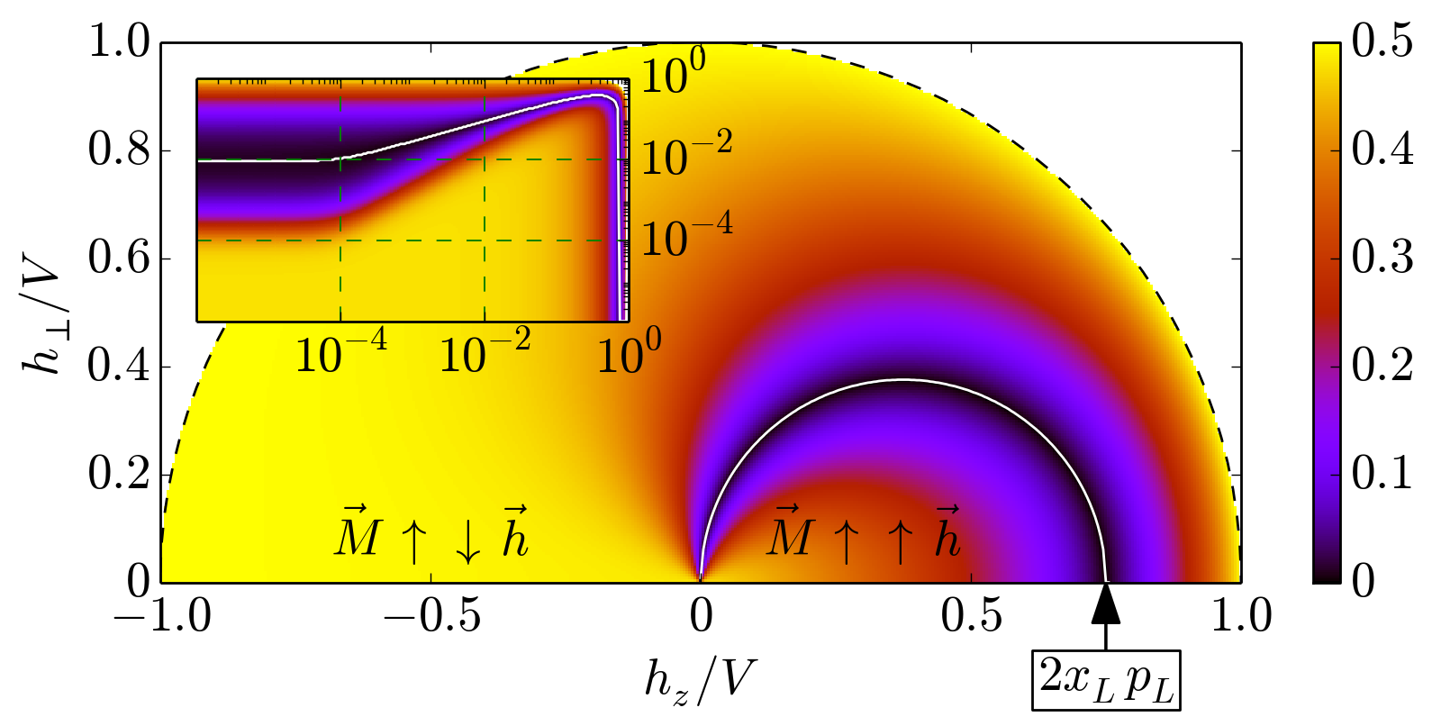
Figure 2: (Color online) The dot magnetization $M$ as function of $h_{z}$ and $h_{\perp}$ for $h<V$ with $x_{L}=x_{R}=\frac{1}{2}$, $p_{L}=p_{R}=\frac{3}{4}$, $J=\frac{1}{100\sqrt{\pi}}$ and $\gamma=10^{-4}V$. The white line indicates $h^{\text{min}}_{\perp}(h_{z})$ where $M$ is minimal. Inset: The same plot on logarithmic scale for $h_{z}>0$.

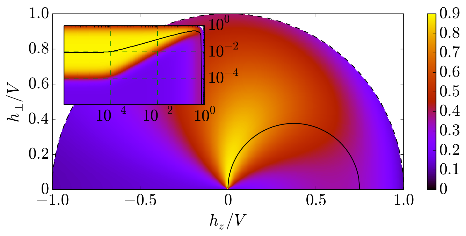
Figure 3: (Color online) The charge current $I/\gamma$ in units of the Korringa rate, analog to Fig. 2. The black line corresponds to the white one of Fig. 2 indicating minimal $M$.

$$M_{z} \approx\frac{1}{2}\frac{p_{L}+p_{R}-2\pi J^{2}x^{2}h_{z}/\gamma}{1+p_{L}p_{R}+x^{2}}\,\,,\,\,x=\frac{h_{\perp}}{\sqrt{h_{z}^{2}+\gamma^{2}}}\,.$$ (6)

At $h=0$ we obtain $M_{0}=M_{h=0}=(1/2)(p_{L}+p_{R})/(1+p_{L}p_{R})$ which, together with $x_{L}+x_{R}=1$, $x_{L}p_{L}=x_{R}p_{R}$ and the value $x_{L}p_{L}$ from the minimum magnetization, determines the four parameters $x_{L,R}$ and $p_{L,R}$ of the fixed point model. The coupling $J$ is related to the Korringa rate which follows from the curvature of the magnetization as function of $h_{\perp}$ at the origin: $(\partial^{2}M/\partial h_{\perp}^{2})_{h=0}=-\gamma^{-2}M_{0}(1+p_{L}p_{R})/(1-p_{L}p_{R})$. Furthermore, for vanishing $h_{\perp}$, the point $h_{z}=0$ can be characterized by a jump of the derivative $(\partial M/\partial h_{z})|_{h=0}$ with a ratio given by the parameters $x_{L,R}$ and $p_{L,R}$, see supplementary material.

Charge current, 2 reservoirs at the fixed point. The charge current $I$ in units of the Korringa rate is shown in Fig. 3. The current is related to the magnetization in a universal way by the formula

$$(I-I_{0})/\gamma =\vec{M}_{\perp}\vec{h}_{\perp}/V$$

$$+(1+p_{L}p_{R})(M_{z}-M_{0})(h_{z}/V-2M_{0})\quad,$$ (7)

with $I_{0}/\gamma=I_{h=0}/\gamma=1/2+(1+p_{L}p_{R})(1-8M_{0}^{2})/4$. At fixed $h_{z}$ the current shows a maximum as function of $h_{\perp}$ at a value roughly of the same order where the magnetization is minimal. This is caused by enhanced inelastic processes increasing the current in this regime. However, since the current varies only slowly in a wide region around the maximum this is not useful to determine the model parameters. An exception is the axis $h_{z}=0$, where the maximum current follows from the formula $I^{\text{max}}_{h_{z}=0}/\gamma=(3+p_{L}p_{R})/4$. Another point of interest is $h=V$ where the magnetization is maximal $\vec{M}=-\vec{h}/(2V)$ (see above). At this point the upper dot level has no occupation and transport happens via elastic cotunneling processes through the lower one. From Eq. (7) we get $I_{h=V}/\gamma=[1-p_{L}p_{R}(2h_{z}^{2}/V^{2}-1)]/4$. For $h_{z}=0$, $h_{\perp}=V$ or $h_{z}=V$, $h_{\perp}=0$ this gives $I/\gamma=(1\pm p_{L}p_{R})/4$. These two values are related to $I^{\text{max}}_{h_{z}=0}$ in a universal way. Together with $I_{0}$ the parameters $p_{L,R}$ and $\gamma$ can be determined and $x_{L,R}$ follow from $x_{L}+x_{R}=1$ and $x_{L}p_{L}=x_{R}p_{R}$. In the quantum interference regime of small magnetic fields the current is shown in the inset of Fig. 3. Analytically the features follow for $h_{z}\lesssim\gamma$ and $h_{\perp}\ll V$ from $(I-I_{0})/\gamma\approx(p_{L}+p_{R})M_{0}x^{2}/(1+p_{L}p_{R}+x^{2})$.

Conclusions. We have shown that the Kondo model with unpolarized leads is generically not the appropriate model to describe the nonequilibrium properties of pseudo-spin-$\frac{1}{2}$ quantum dots in the Coulomb blockade regime. Noncollinear spin orientations in effective reservoirs give rise to characteristic features as function of an applied magnetic field in the strong nonequilibrium regime independent of the microscopic details of the model, even away from the fixed point. These features are experimentally accessible. For future research it is of high interest to characterize the universal properties of the model also in the strong coupling regime $V\sim T_{K}$ where more refined techniques have to be used frg_noneq ; strong_coupling_RTRG ; smirnov_grifoni_03 .

This work was supported by the DFG via FOR 723 and 912. We thank V. Meden, M. Pletyukhov, D. Schuricht, and M. Wegewijs for valuable discussions.

References

- (1) R. Hanson et al., Rev. Mod. Phys. 79, 1217 (2007).
- (2) S. Andergassen et al., Nanotechnology 21, 272001 (2010).
- (3) L. I. Glazman and M. E. Raikh, Sov. Phys. JETP Lett. 47, 452 (1988); T. K. Ng and P. A. Lee, Phys. Rev. Lett. 61, 1768 (1988).
- (4) D. Goldhaber-Gordon et al., Nature (London) 391, 156 (1998); S. M. Cronenwett, T. H. Oosterkamp, and L. P. Kouwenhoven, Science 281, 540 (1998); F. Simmel et al., Phys. Rev. Lett. 83, 804 (1999).
- (5) T. A. Costi, A. C. Hewson, and V. Zlatic, J. Phys.: Condens. Matter 6, 2519 (1994).
- (6) L. I. Glazman and M. Pustilnik, in Nanophysics: Coherence and Transport (H. Bouchiat et al., Elsevier, 2005) p. 427.
- (7) A. Rosch, J. Kroha and P. Wölfle, Phys. Rev. Lett. 87, (2001) 156802; A. Rosch et. al, Phys. Rev. Lett. 90, 076804 (2003).
- (8) S. Kehrein, Phys. Rev. Lett. 95, 056602 (2005); P. Fritsch and S. Kehrein, Phys. Rev. B 81, 035113 (2010).
- (9) H. Schoeller, Eur. Phys. J. Special Topics 168, 179 (2009).
- (10) H. Schoeller and F. Reininghaus, Phys. Rev. B 80, 045117 (2009); ibid. Phys. Rev. B 80, 209901(E) (2009).
- (11) M. Pletyukhov, D. Schuricht, and H. Schoeller, Phys. Rev. Lett. 104, 106801 (2010).
- (12) S. G. Jakobs, M. Pletyukhov, and H. Schoeller, Phys. Rev. B 81, 195109 (2010); J. Eckel et al., New J. Phys. 12, 043042 (2010).
- (13) M. Pletyukhov and H. Schoeller, Phys. Rev. Lett. 108, 260601 (2012); F. Reininghaus, M. Pletyukhov and H. Schoeller, Phys. Rev. B 90, 085121 (2014).
- (14) S. Smirnov and M. Grifoni, Phys. Rev. B 87, 121302(R) (2013); ibid, New J. Phys. 15, 073047 (2013).
- (15) A. V. Kretinin, H. Shtrikman, and D. Mahalu, Phys. Rev. B 85, 201301(R) (2012); O. Klochan et al., Phys. Rev. B 87, 201104(R) (2013).
- (16) J. Martinek et al., Phys. Rev. Lett. 91, 127203 (2003); J. Martinek et al., Phys. Rev. Lett. 91, 247202 (2003); M. Sindel et al., Phys. Rev. B 76, 045321 (2007).
- (17) D. Boese, W. Hofstetter, and H. Schoeller, Phys. Rev. B 64, 125309 (2001); ibid. Phys. Rev. B 66, 125315 (2002).
- (18) V. Kashcheyevs et al., Phys. Rev. B 75, 115313 (2007).
- (19) J. König, and J. Martinek, Phys. Rev. Lett. 90, 166602 (2003); M. Braun, J. König, and J. Martinek, Phys. Rev. B 70, 195345 (2004); I. Weymann and J. Barnas, Phys. Rev. B 75, 155308 (2007).
- (20) J. Paaske, A. Andersen, and K. Flensberg, Phys. Rev. B 82, 081309(R) (2010).
- (21) M. Pletyukhov and D. Schuricht, Phys. Rev. B 84, 041309 (2011).
- (22) T. Korb et al., Phys. Rev. B 76, 165316 (2007).