Abstract

Virasoro irregular conformal block is presented as the expectation value of Jack-polynomials of the beta-deformed Penner-type matrix model and is compared with the inner product of Gaiotto states with arbitrary rank. It is confirmed that there are non-trivial modifications of the Gaiotto states due to the normalization of the states. The relation between the two is explicitly checked for rank 2 irregular conformal block.

1 Introduction

Virasoro irregular module appears in connection with the N=2 super-Yang Mills theory [1]. The irregular module so called Gaiotto state or Whittaker state [2] is the simultaneous eigenstate of the positive Virasoro generators. The irregular module is constructed as the superposition of one primary state and its descendents [1, 3].

On the other hand, the irregular module is also constructed as the colliding limit of primary operators as shown in [4]. The colliding limit is the fusion of primary vertex operators with the addition of Heisenberg-coherent modes. As a result, the state becomes the simultaneous eigenstate of positive Virasoro operators, i.e. the irregular module.

Will the two different approaches produce the same result? In this paper we like to answer this question. We will confine ourselves to the case with the Gaiotto sate $|I_{n}\rangle$ of rank $n\geq 1$, simultaneous eigenstate of $L_{n},L_{n+1},\cdots,L_{2n}$. In section 2, Gaiotto state of rank $n$ constructed in [5] is summarized and its inner product is investigated. The inner product is important since it contains all the information of descendents in the Gaiotto state. In section 3, a differently looking form of the inner product is provided using the colliding limit of the regular conformal correlation. The result is given in terms of the beta-deformed Penner-type matrix model. Since the random matrix model is the result of the fusion of primary operators, the partition function should produce the colliding limit of the conformal block, which we call the (two-point) irregular conformal block (ICB). A simple and clear way to obtain ICB is presented with the help of the loop equation and ICB is compared with the inner product of Gaiotto states. We pinpoint the non-trivial modification from the Gaiotto state in [5]. The summary and discussion are given in section 4 and some detailed calculation is given in the appendix.

2 Virasoro irregular module and its inner product

The irregular state is explicitly constructed for rank 1 in [1, 3] and for rank $n$ in [5]. We will use the convention $|\widetilde{G_{2n}}\rangle$ for Gaiotto state with rank $n$ following [5] (another form is also found in [6]), whereas we reserve $|I_{n}\rangle$ for the state obtained from the colliding limit given in [4].

$$|\widetilde{G_{2n}}\rangle=\sum_{\ell,Y,\ell_{p}}\Lambda^{\ell/n}\left\{\prod_{i=1}^{n-1}a_{i}^{\ell_{2n-i}}b_{i}^{\ell_{i}}\right\}m^{\ell_{n}}Q_{\Delta}^{-1}\Big{(}1^{\ell_{1}}2^{\ell_{2}}\cdots(2n-1)^{\ell_{2n-1}}(2n)^{\ell_{2n}};Y\Big{)}L_{-Y}|\Delta\rangle\,,$$ (2.1)

where $L_{-Y}=L_{Y}^{+}$ represents the product of lowering operators and $L_{Y}=L_{1}^{\ell_{1}}L_{2}^{\ell_{2}}\cdots L_{s}^{\ell_{s}}$. $|\Delta\rangle$ is the primary state with conformal dimension $\Delta$ and $Q_{\Delta}(Y;Y^{\prime})$ is the shorthand notation of $\langle\Delta|L_{Y^{\prime}}L_{-Y}|\Delta\rangle$. The summation $\ell$ runs from 0 to $\infty$, $Y$ and $\ell_{p}$ maintaining $|Y|=\ell$ and $\sum p\ell_{p}=\ell$.

One can confirm that $|\widetilde{G_{2n}}\rangle$ is the simultaneous eigenstate; $L_{k}|\widetilde{G_{2n}}\rangle=\Lambda^{k/n}a_{2n-s}$ for $n<k\leq 2n$ and $L_{n}|\widetilde{G_{2n}}\rangle=\Lambda m|\widetilde{G_{2n}}\rangle$ from the expectation values for $W=1^{\ell_{1}}2^{\ell_{2}}\cdots(2n)^{\ell_{2n}}$,

$$\langle\Delta|L_{W}L_{2n-s}|\widetilde{G_{2n}}\rangle=\Lambda^{2n-s/n}a_{s}\langle\Delta|L_{W}|\widetilde{G_{2n}}\rangle~{}~{}~{}~{}{\rm for}~{}0\leq s<n,$$

$$\langle\Delta|L_{W}L_{n}|\widetilde{G_{2n}}\rangle=\Lambda m\langle\Delta|L_{W}|\widetilde{G_{2n}}\rangle\,,$$ (2.2)

with $a_{0}\equiv 1$. Here, the eigenvalues are given in terms of $\Lambda$, $a_{i}$’s and $m$ only. The other coefficients $b_{i}$’s are not fixed by the eigenvalues but enter in the inner product since

$$\langle\Delta|L_{W}|\widetilde{G_{2n}}\rangle=\Lambda^{\ell/n}\left\{\prod_{i=1}^{n-1}a_{i}^{\ell_{2n-i}}b_{i}^{\ell_{i}}\right\}m^{\ell_{n}}\,.$$ (2.3)

Note that inner product contains all the information on the descendents. Thus, one may assume that $b_{i}$’s are related with the contribution of descendents. To find out further information of $b_{i}$’s, we need to resort to other procedures.

3 Irregular conformal block and colliding limit

The inner product can be evaluated using the idea of colliding limit of the multi-point regular conformal correlation introduced in [7, 4, 6]. We follow the procedure appeared in [8]. Let us consider the conformal part of $n+2$ primary operator correlation with $N$ screening operators. If one fuses $n+1$ operators at the origin with the colliding limit, one ends up with the $\beta$-deformed Penner-type partition function

$$Z_{(0:n)}(c_{0};\{c_{k}\})=\int\prod_{i=1}^{N}d\lambda_{i}~{}\Delta(\lambda)^{2\beta}~{}e^{-\frac{\sqrt{\beta}}{g}\sum_{i}V(\lambda_{i};c_{0},\{c_{k}\})}\,,$$ (3.1)

where $\Delta(\lambda)=\prod_{i<j}(\lambda_{i}-\lambda_{j})$ is the Vandermonde determinant and $\beta=-b^{2}$ (or $b=i\sqrt{\beta}$) with the screening charge $b$. The Penner-type potential is given as the sum of logarithmic and inverse power terms

$$\frac{1}{\hbar}V_{(0:n)}(z;c_{0},\{c_{k}\})=-c_{0}\log z+\sum_{k=1}^{n}\frac{c_{k}}{kz^{k}}\,.$$ (3.2)

(One may identify $c_{k}=\sum_{r=1}^{n}\alpha_{r}(z_{r})^{k}$ where $\alpha_{r}$ is the Liouville charge of the primary operator at $z_{r}$. Since the colliding limit corresponds to $z_{r}\to 0$ and $\alpha_{r}\to\infty$ so that $c_{k}$ is ensured finite, one may consider the limit as the ideal multi-pole expansion. In addition, we use the notation $g=i\hbar/2$ so that $\sqrt{\beta}/g=-2b/\hbar$.)

We remark by passing that the integration range of the partition function is naturally given as $0$ to $\infty$. Before the colliding limit one usually chooses the integration range between the positions of the primary operators. For example, one may choose the position of the primary operators as ($0,z_{1}=z,z_{2}=1,\infty$) and chooses the integration ranges from $0$ to $z_{1}$ or from $z_{2}$ to $\infty$. However, to have the proper colliding limit, one needs to choose the integration range from $z_{1}$ to $z_{2}$ and take the limit $z_{1}\to 0$ and $z_{2}\to\infty$.

Let us introduce the primary state $|\Delta\rangle$ with conformal dimension $\Delta=c_{0}(Q-c_{0})$ in the presence of the background charge $Q$. Then $\langle\Delta|$ is the primary state with the conformal dimension $\Delta=c_{\infty}(Q-c_{\infty})$ where $c_{\infty}$ is fixed by the neutrality condition $c_{0}+c_{\infty}+bN=Q$. The colliding limit introduces the irregular state $|I_{n}\rangle$ and the partition function is identified with the inner product $Z_{(0:n)}(c_{0};\{c_{k}\})=\langle\Delta|I_{n}\rangle$. This ensures that the irregular state $|I_{n}\rangle$ is dependent on the set of coefficients $\{c_{1},\cdots c_{n}\}$. In fact, it is demonstrated in [4] that the coefficient $c_{k}$ is the coherent coordinate of Heisenberg mode $a_{k}$, $a_{k}|I_{n}\rangle=c_{k}|I_{n}\rangle$.

Since $|I_{n}\rangle$ is the simultaneous eigenstate of $L_{n},L_{n+1},\cdots,L_{2n}$ generators, their eigenvalues can be parametrized as $\Lambda_{k}=(k+1)Qc_{k}-\sum_{p=0}^{k}c_{p}c_{k-p}$ with $k=n,\cdots,2n$. However, the eigenstate condition is not enough to fix $|I_{n}\rangle$ as seen in (2.3) and needs the information on the descendents in $|I_{n}\rangle$. Note that the lower positive generators $L_{k}$ ($k=1,\cdots,n-1$) obeying $\left[L_{k},L_{n}\right]=(k-n)L_{k+n}$. An easy way to realize this non-commutative properties is to represent $L_{k}$ as the differential form of the coherent coordinates $c_{k}$’s. Putting $\mathcal{L}_{k}=\Lambda_{k}+v_{k}$, one has

$$v_{k}\equiv\sum_{\ell\in\mathbb{N}}\ell~{}c_{\ell+k}~{}\frac{\partial}{\partial c_{\ell}}$$ (3.3)

and the consistency condition

$$[v_{k},v_{\ell}]\langle\Delta|I_{n}\rangle=(\ell-k)~{}v_{\ell+k}\langle\Delta|I_{n}\rangle\,.$$ (3.4)

It should be noted that the Gaiotto state $|\widetilde{G_{2n}}\rangle$ in (2.1) satisfies the consistence condition trivially since $v_{k}\langle\Delta|\widetilde{G_{2n}}\rangle=0$.

One can find the parameter dependence for the rank 1 simply by scaling the integration variable $\lambda_{i}\to c_{1}\lambda_{i}$ to get $Z_{(0:1)}(c_{0};c_{1})=c_{1}^{-bN(bN+2c_{0}-Q)}Z_{(0:1)}(c_{0};1)$. However, for the rank higher than 1, one needs more complicated process. The easiest way to find the parameter dependence is to use the loop equation of the matrix model. The loop equation has the form [8]

$$\sum_{k=0}^{n-1}\frac{v_{k}(\log(Z_{(0:n)}))}{z^{2+k}}=-\frac{\xi(z)}{\hbar^{2}}\,,$$ (3.5)

where $v_{0}$ conforms to the notation of (3.3), $v_{0}\equiv\sum_{\ell\in\mathbb{N}}\ell\,c_{\ell}\,\frac{\partial}{\partial c_{\ell}}$ and $\xi(z)=4W(z)^{2}-4W(z)V^{\prime}(z)+2\hbar QW^{\prime}(z)-\hbar^{2}W(z,z)$. Here $W(z)$ is the resolvent $W(z)=\hbar b/2\langle 1/(z-\lambda_{i})\rangle$, and $W(z,z)$ is the connected two-point resolvent $W(z,z)=-b^{2}\langle\sum_{i,j}1/(z-\lambda_{i})(z-\lambda_{j})\rangle_{c}$. The prime stands for the differentiation.

One may view that the loop equation provides the energy momentum expectation value $\varphi_{2}(z)$, which encodes the Seiberg-Witten curve [9, 10, 11, 1]. Putting $\varphi_{2}(z)=\sum_{n\leq k\leq 2n}\Lambda_{k}/z^{2+k}+\sum_{0\leq kn-1}{\cal L}_{k}/z^{2+k}$, one has the relation with the resolvent according to the loop equation: $\varphi_{2}(z)=(2W-V^{\prime})^{2}+\hbar Q(2W-V^{\prime})^{\prime}-\hbar^{2}W(z,z)$. Large $z$ expansion of the loop equation eventually reduces to the flow equation

$$v_{k}(\log Z_{(0:n)})=d_{k}^{(0:n)}(\{c_{k}\})\,,$$ (3.6)

where $d_{k}^{(0:n)}$ is the moment of $\xi(z)$; $\oint dzz^{1+k}\xi(z)/(-\hbar^{2}2\pi i)$. The flow equation satisfies the consistency condition (3.4) automatically whose explicit solutions can be found in [8, 12].

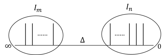
Figure 1: Schematic diagram of $\left\langle{I_{m}|I_{n}}\right\rangle$ from the colliding limit

The idea can be extended to find the inner product $\langle I_{m}|I_{n}\rangle$ from the colliding limit of $(m+n+2)$-point correlation (see figure 1). Fusing $n+1$ primary operators at the origin and $m+1$ operators at infinity, one has the partition function $Z_{(m:n)}$

$$Z_{(m:n)}(c_{0};\{c_{k}\};\{c_{-\ell}\})=\int\prod_{i=1}^{N}d\lambda_{i}\Delta(\lambda)^{2\beta}e^{-\frac{\sqrt{\beta}}{g}\sum_{i}V_{(m:n)}(\lambda_{i};c_{0},\{c_{k}\},\{c_{-\ell}\})}\,,$$

$$\frac{1}{\hbar}V_{(m:n)}(z;c_{0},\{c_{k}\},\{c_{-\ell}\})=-c_{0}\log z+\sum_{k=1}^{n}\left(\frac{{c_{k}}}{kz^{k}}\right)+\sum_{\ell=1}^{m}\left(\frac{c_{-\ell}~{}z^{\ell}}{\ell}\right)\,.$$ (3.7)

The partition function is related with the inner product $\langle I_{m}|I_{n}\rangle$. However, there is a subtlety, so called $U(1)$ contribution. This factor comes from the limiting procedure: It is noted that as $z_{a}\to\infty$ and $z_{b}\to 0$ one has the finite contribution $\prod_{a,b}(1-z_{b}/z_{a})^{-{2\alpha_{a}\alpha_{b}}}\to e^{\zeta_{(m:n)}}$, where $\zeta_{(m:n)}=\sum_{k}^{{\rm min}(m,n)}2c_{k}c_{-k}/k$. Therefore, one has the inner product of the form $\langle I_{m}|I_{n}\rangle=e^{\zeta_{(m:n)}}Z_{(m:n)}(c_{0};\{c_{k}\};\{c_{-\ell}\})$.

The inner product between the two irregular modules inherits the property of the conformal block of the regular multi-correlation. Considering the colliding limit, one may define the irregular conformal block ${\cal F}_{\Delta}^{(m:n)}$ as the inner product of the irregular modules with appropriate normalization: ${\cal F}_{\Delta}^{(m:n)}={\langle I_{m}|I_{n}\rangle}/({\langle I_{m}|\Delta\rangle~{}\langle\Delta|I_{n}\rangle})$ whose conformal dimension is given as $\Delta=(c_{0}+N_{0})(Q-c_{0}-N_{0})=(c_{\infty}+N_{\infty})(Q-c_{\infty}-N_{\infty})$ [12].

In this spirit, one may naturally define ICB using the $\beta$ deformed Penner-type matrix model as the following:

$${\cal F}_{\Delta}^{(m:n)}(\{c_{-\ell}\}:\{c_{k}\})=\frac{e^{\zeta_{(m:n)}}Z_{(m:n)}(c_{0};\{c_{k}\};\{c_{-\ell}\})}{Z_{(0:n)}(c_{0};\{c_{k}\})Z_{(0:m)}(c_{\infty};\{c_{-\ell}\})}\,,$$ (3.8)

where $Z_{(0:n)}(c_{0};\{c_{k}\})$ and $Z_{(0:m)}(c_{\infty};\{c_{-\ell}\})$ provide the proper normalization for the irregular conformal block. Here we use the change of variable $\lambda_{i}\to 1/\lambda_{i}$ to express $\langle I_{m}|\Delta\rangle$ as $Z_{(0:m)}(c_{\infty};\{c_{-\ell}\})$.

To evaluate ICB we note that the potential $V_{(m:n)}$ contains the information of the irregular module at the origin and at infinity at the same time. Therefore, each module can be derived if one views the same potential on a different footing. The information of the irregular module at the origin is obtained if one regards the potential $V_{0}=V_{(0:n)}(\{\lambda_{i}\};c_{0},\{c_{k}\})$ as the reference one and $\Delta V_{0}$ as its perturbation:

$$\frac{1}{\hbar}V_{0}=\sum_{I=1}^{N_{0}}\Big{(}-c_{0}\log\lambda_{I}+\sum_{k=1}^{n}\frac{c_{k}}{k}\lambda_{I}^{-k}\Big{)}\,;~{}~{}~{}\frac{1}{\hbar}\Delta V_{0}=\sum_{I=1}^{N_{0}}\Big{(}\sum_{\ell=1}^{n}\frac{c_{-\ell}}{\ell}{\lambda_{I}^{\ell}}\Big{)}\,.$$ (3.9)

That is, $V_{0}$ is the potential for the partition function $Z_{(0:n)}$ with $N_{0}(\leq N)$ number of screening operators. At infinity one has the reference potential $\sum_{J=1}^{N_{\infty}}\Big{(}-c_{0}\log\lambda_{J}+\sum_{\ell=1}^{n}{c_{-\ell}}{\lambda_{i}^{\ell}}/\ell\Big{)}$ and its perturbation $\sum_{J=1}^{N_{\infty}}\Big{(}\sum_{k=1}^{n}{c_{k}}\lambda_{J}^{-k}/k\Big{)}$. We introduce the number $N_{\infty}$ of screening operators at infinity so that $N_{\infty}+N_{0}=N$. One may rewrite the potential in a familiar form if one changes the variable $\lambda_{J}\to 1/\mu_{J}$ to get the equivalent potential

$$\frac{1}{\hbar}V_{\infty}=\sum_{J=1}^{N_{\infty}}\Big{(}-c_{\infty}\log\mu_{J}+\sum_{\ell=1}^{m}\frac{c_{-\ell}}{\ell}\mu_{\!J}^{-\ell}\Big{)}\,;~{}~{}~{}~{}\frac{1}{\hbar}\Delta V_{\infty}=\sum_{J=1}^{N_{\infty}}\Big{(}\sum_{k=1}^{n}\frac{c_{k}}{k}\mu_{\!J}^{k}\Big{)}\,.$$ (3.10)

In this way the perturbative potential and the cross terms in the Vandermonde determinant provide ICB :

$${\cal F}_{\Delta}^{(m:n)}(\{c_{-\ell}\}:\{c_{k}\})=e^{\zeta_{(m:n)}}\Big{\langle}\prod_{I,J}(1-\lambda_{I}\mu_{J})^{2\beta}e^{-\frac{\sqrt{\beta}}{g}(\Delta V_{0}(\lambda_{I})+\Delta V_{\infty}(\mu_{J}))}\Big{\rangle}\,,$$ (3.11)

where the bracket denotes the expectation value using the reference partition function:

$$\langle{\mathcal{O}}(\lambda_{I})\rangle\equiv\langle{\mathcal{O}}\rangle_{+}=\Big{(}Z_{(0:n)}(c_{0};\{c_{k}\})\Big{)}^{-1}\int\prod_{I=1}^{N_{0}}d\lambda_{I}\Delta(\lambda)^{2\beta}{\mathcal{O}}(\lambda_{I})e^{-\frac{\sqrt{\beta}}{g}\sum_{i}V_{0}(\lambda_{I})}\,,$$ (3.12)

$$\langle{\mathcal{O}}(\mu_{J})\rangle\equiv\langle{\mathcal{O}}\rangle_{-}=\Big{(}Z_{(0:m)}(c_{\infty};\{c_{\ell}\})\Big{)}^{-1}\int\prod_{J=1}^{N_{\infty}}d\mu_{J}\Delta(\mu)^{2\beta}{\mathcal{O}}(\mu_{J})e^{-\frac{\sqrt{\beta}}{g}\sum_{i}V_{\infty}(\mu_{J})}\,,$$

which can be regarded as the generalization of Selberg integral [14, 15]. One may put ICB in (3.11) compactly in terms of Jack polynomial [16, 17]. Putting $p_{k}=\sum_{I}\lambda_{I}^{k}$ and $p^{\prime}_{k}=\sum_{J}\mu_{\!J}^{k}$, one has the identity

$$\prod_{I,J}(1-\lambda_{I}\mu_{J})^{2\beta}e^{-\frac{\sqrt{\beta}}{g}(\Delta V_{0}(\lambda_{I})+\Delta V_{\infty}(\mu_{J}))}$$

$$~{}~{}~{}~{}~{}~{}~{}~{}~{}~{}=\exp\big{\{}-\beta\sum_{k=1}^{\infty}\frac{1}{k}p_{k}(p^{\prime}_{k}-\tilde{c}_{-k})\big{\}}\times\exp\big{\{}-\beta\sum_{k=1}^{\infty}\frac{1}{k}p^{\prime}_{k}(p_{k}-\tilde{c}_{k})\big{\}}\,,$$ (3.13)

where $\tilde{c}_{\pm k}=i2c_{\pm k}/\sqrt{\beta}=-2c_{\pm k}/b$, (and $\tilde{c}_{k}=0$ for $k>n$ and $\tilde{c}_{-k}=0$ for $k>m$). Using the Cauchy-Stanley identity [18, 19] $e^{\beta\sum_{k\geq 1}\frac{1}{k}p_{k}p^{\prime}_{k}}=\sum_{R}j_{R}^{(\beta)}(p)j_{R}^{(\beta)}(p^{\prime})$, one has ICB as

$${\cal F}_{\Delta}^{(m:n)}=e^{\eta_{(m:n)}}\sum_{Y,W}\Big{\langle}j_{Y}^{(\beta)}(p_{k})j_{W}^{(\beta)}(-p_{k}+\tilde{c}_{k})\Big{\rangle}_{+}\Big{\langle}j_{Y}^{(\beta)}(-p^{\prime}_{k}+\tilde{c}_{-k})j_{W}^{(\beta)}(p^{\prime}_{k})\Big{\rangle}_{-}\,\,.$$ (3.14)

The explicit form of the general ICB is not available yet. Here we check a few non-trivial terms using the resolvent in the loop equation of the reference partition function. Each term can be obtained from the large $z$ expansion of the resolvent $W(z)$. The details of calculation are given in the appendix. ICB is given in power of $\eta_{0}\equiv c_{1}c_{-1}$, which is compatible with the Young diagram expansion. For the rank 1, up to order ${\mathcal{O}}(\eta_{0}^{2})$ one has

$${\cal F}_{\Delta}^{(1:1)}=1+\eta_{0}\frac{2\bar{c_{0}}\bar{c_{\infty}}}{\Delta}+\eta_{0}^{2}\frac{{4\bar{c_{0}}^{2}\bar{c_{\infty}}^{2}c}/{\Delta}+4\Delta+2+12(\bar{c_{0}}^{2}+\bar{c_{\infty}}^{2})+32\bar{c_{0}}^{2}\bar{c_{\infty}}^{2}}{c+2c\Delta+2\Delta(8\Delta-5)}\,,$$ (3.15)

where $\bar{c_{0}}=Q-c_{0}$, $\bar{c_{\infty}}=Q-c_{\infty}$, $c=1+6Q^{2}$. Comparing this with the Gaiotto inner product up to ${\mathcal{O}}(\Lambda\Lambda^{\prime})^{2}$ (using (2.1) with $\langle\widetilde{G}_{2}|$ using the primed notation)

$$\langle\widetilde{G_{2}}|\widetilde{G_{2}}\rangle=1+\Lambda\Lambda^{\prime}\frac{mm^{\prime}}{2\Delta}+(\Lambda\Lambda^{\prime})^{2}\frac{{m^{2}m^{\prime 2}c}/{4\Delta}+4\Delta+2-3(m^{2}+m^{\prime 2})+2m^{2}m^{\prime 2}}{c+2c\Delta+2\Delta(8\Delta-5)}\,,$$ (3.16)

we find $\Lambda^{2}=-c_{1}^{2}$ and $m\Lambda=2c_{1}\bar{c_{0}}$, consistent with the eigenvalues of $L_{2}$ and $L_{1}$.

Non-trivial check is given for the rank 2. Matrix model provides ${\cal F}_{\Delta}^{(1:2)}$ up to ${\mathcal{O}}\left(\eta_{0}^{2}\right)$

$${\cal F}_{\Delta}^{(1:2)}=1+\eta_{0}\frac{\bar{b}_{1}\bar{c_{\infty}}}{\Delta}$$

$$~{}~{}~{}+\eta_{0}^{2}\frac{c\,\bar{c_{\infty}}^{2}\,\bar{b}_{2}/\Delta+c_{2}(2+12\bar{c_{\infty}}^{2}+4\Delta)(1-(Q+2\bar{c_{0}})/c_{1}^{2})+(3+8\bar{c_{\infty}}^{2})\,\bar{b}_{2}}{c+2c\Delta+2\Delta(8\Delta-5)}\,,$$ (3.17)

where $c_{1}\bar{b}_{1}=(d_{1}^{(0:2)}+2\bar{c_{0}}c_{1})$, $c_{1}^{2}\,\bar{b}_{2}=(d_{1}^{(0:2)}+2\bar{c_{0}}c_{1})^{2}+c_{2}\,\partial\,d_{1}^{(0:2)}/\partial c_{1}$. The explicit form of $d_{1}^{(0:2)}$ is found in (B.1). On the other hand, one has the Gaiotto inner product up to ${\mathcal{O}}(\Lambda^{\prime}\sqrt{\Lambda})^{2}$

$$\langle\widetilde{G_{2}}|\widetilde{G_{4}}\rangle=1+\Lambda^{\prime}\sqrt{\Lambda}\frac{m^{\prime}b_{1}}{2\Delta}+(\Lambda^{\prime}\sqrt{\Lambda})^{2}\frac{{cm^{\prime 2}b_{1}^{2}}/(4\Delta)+(2-3m^{\prime 2}+4\Delta)m+(-3+2m^{\prime 2})b_{1}^{2}}{c+2c\Delta+2\Delta(8\Delta-5)}\,.$$ (3.18)

Comparing the two we obtain the parameter relations $\Lambda^{\prime 2}=-c_{-1}^{2}$, $m^{\prime}\Lambda^{\prime}=2c_{-1}\bar{c_{\infty}}$ and $\Lambda m=-c_{1}^{2}-2c_{2}(\bar{c_{0}}-Q/2)$, the eigenvalues of $L_{1}$, $L_{2}$. However $\bar{b}_{2}$ is not $\bar{b}_{1}^{2}$ in (3.17) which is different from (3.18). Therefore, $(\sqrt{\Lambda}\,b_{1})^{\ell}$ cannot be considered as a simple constant but should be of the form $(c_{1}\,\bar{b}_{1})^{\ell}=\frac{1}{Z_{(0:2)}}(\Lambda_{1}+v_{1})^{\ell}Z_{(0:2)}$.

One can check this relation holds for ${\mathcal{F}}_{\Delta}^{(2:2)}$ if the Gaiotto inner product

$$\begin{split}\langle\widetilde{G_{4}}|\widetilde{G_{4}}\rangle=1&+(\Lambda^{\prime}\Lambda)^{1/2}\frac{b_{1}b^{\prime}_{1}}{2\Delta}+\frac{\Lambda^{\prime}\Lambda}{c+2c\Delta+2\Delta(8\Delta-5)}\biggl{[}\frac{c\,b_{1}^{2}{b^{\prime}}_{1}^{2}}{4\Delta}\\ &+2(b_{1}^{2}{b^{\prime}}_{1}^{2}+mm^{\prime})-3(m{b^{\prime}}_{1}^{2}+3m^{\prime}b_{1}^{2})+4\Delta mm^{\prime}\biggr{]}+(\Lambda^{\prime}\Lambda)^{3/2}\end{split}$$ (3.19)

is compared with the matrix result given in (B.7). Additional identification of $b_{1}^{\prime}$ with $\bar{b}_{-1}$ appears as it should be, where $(c_{-1}\,\bar{b}_{-1})^{\ell}=\frac{1}{Z_{(0:2)}}(\Lambda_{-1}+v_{-1})^{\ell}Z_{(0:2)}$.

4 Summary and discussion

We found the Virasoro irregular conformal block using the beta deformed Penner type matrix model and present the result in terms of the expectation values of the Jack polynomial (3.14). We check ICB explicitly for a few ranks and compare with the inner product of Gaiotto state proposed by [5]. There is a non-trivial modification between the two results due to the difference of the normalization as is suggested in [5].

Referring to the explicit check given for the rank 1 and 2, we can clearly see that the Gaiotto state needs to be modified to represent the colliding limit of the conformal correlation. Note that the expectation value $\langle\Delta|L_{k}^{\ell_{k}}|\widetilde{G_{2n}}\rangle$ is $(\Lambda^{k/n}b_{k})^{\ell_{k}}$ according to (2.3). On the other hand, $|I_{n}\rangle$ has the $L_{k}^{\ell_{k}}$ expectation value $\Big{(}(\Lambda_{k}+v_{k})^{\ell_{k}}Z_{(0:n)}\Big{)}/Z_{(0:n)}$. Therefore, one may conclude that the Gaiotto state should be modified by using the coefficient relation $(\Lambda^{k/n}b_{k})^{\ell_{k}}\to\Big{(}(\Lambda_{k}+v_{k})^{\ell_{k}}Z_{(0:n)}\Big{)}/Z_{(0:n)}$. Considering $\langle\Delta|L_{1}^{\ell_{1}}L_{2}^{\ell_{2}}|I_{n}\rangle=(\Lambda_{2}+v_{2})^{\ell_{2}}(\Lambda_{1}+v_{1})^{\ell_{1}}Z_{(0:n)}$, one has

$$\langle\Delta|L_{W}|I_{n}\rangle=\Lambda^{\ell/n}m^{\ell_{n}}\left\{\prod_{i=1}^{n-1}a_{i}^{\ell_{2n-i}}\right\}\left\{\left(\Lambda_{n-1}+v_{n-1}\right)^{\ell_{n-1}}\cdots\left(\Lambda_{1}+v_{1}\right)^{\ell_{1}}{Z_{(0:n)}}\right\}$$ (4.1)

with proper ordering. The case of rank 1 is trivial since there is no $b_{k}$’s.

In the paper we consider mainly the two-point ICB. One may extend the result to $N$-point ICB $\langle\prod_{A=1}^{N}I_{m_{A}}(z_{A})\rangle$ by generalizing the potential in (3.7):

$$\frac{1}{\hbar}V_{(\{m_{A}\})}(z;\{c_{0}^{(A)}\},\{c_{k}^{(A)}\})=\sum_{A=1}^{N}\left\{-c_{0}^{(A)}\log(z-z_{A})+\sum_{k=1}^{n_{A}}\left(\frac{{c_{k}^{(A)}}}{k(z-z_{A})^{k}}\right)\right\}\,.$$ (4.2)

ICB will be given with the appropriate normalization at each point, i.e., by treating the potential as the sum of the reference potential and perturbation at each point.

Noting the Penner-type matrix model provides ICB, one may wonder if there exists another systematic way of obtaining the irregular conformal block of arbitrary rank from regular conformal block, as seen in the rank 1 case [3] or for $SU(N)$ in [20] by decoupling a certain large mass limit. However, such a decoupling limit is not achieved yet for rank greater than $1$. It will be interesting to find the limit using the relation of the Selberg integral with the Jack polynomials to have (3.14).

In addition, one may have the colliding limit for W-algebraic symmetry as done in [5] using $SU(N)$ Toda theories. The corresponding matrix model is straight-forward generalization of the Virasoro symmetric case for $SU(N)$. Making use of [21], we have

$$Z_{(m:n)}^{SU(N)}=\int\prod_{a=1}^{N-1}\prod_{i=1}^{N_{a}}d\lambda_{i}^{(a)}\Delta(\lambda^{(a)})^{2\beta}\prod_{a=1}^{N-2}\Delta(\lambda^{(a)},\lambda^{(a+1)})^{-\beta}e^{-\frac{\sqrt{\beta}}{g}\sum_{a=1}^{N-1}\sum_{i=1}^{N_{a}}V_{(m:n)}^{(a)}(\lambda_{i})}\,,$$

$$\frac{1}{\hbar}V_{(m:n)}^{(a)}(z)=-c_{0}^{(a)}\log z+\sum_{k=1}^{n}\left(\frac{{c_{k}^{(a)}}}{kz^{k}}\right)+\sum_{\ell=1}^{m}\left(\frac{c_{-\ell}^{(a)}~{}z^{\ell}}{\ell}\right)\,,$$ (4.3)

with $c_{k}^{(a)}=\sum_{r=1}^{n}(\alpha_{r},e_{a})(z_{r})^{k}$, and $c_{-\ell}^{(a)}=\sum_{r=1}^{m}(\tilde{\alpha}_{r},e_{a})(\tilde{z}_{r})^{-\ell}$. Here $e_{a}$ are the simple roots of $SU(N)$. This leads to the $SU(N)$ ICB:

$${\cal F}_{\Delta}^{(m:n)}=e^{\zeta_{(m:n)}}\sum_{\vec{Y}}\left\langle\prod_{a=1}^{N}j^{(\beta)}_{Y_{a}}(p_{k}^{(a-1)}-p_{k}^{(a)}+\tilde{c}_{k}^{(a)})\right\rangle_{\!\!+}\left\langle\prod_{a=1}^{N}j^{(\beta)}_{Y_{a}}(p_{k}^{\prime(a)}-p_{k}^{\prime(a-1)}+\tilde{c}_{-k}^{(a)})\right\rangle_{\!\!-}$$ (4.4)

with $\tilde{c}_{-k}^{(a)}=2\sum_{s=1}^{a-1}c_{-k}^{(s)}/b$, $\tilde{c}_{k}^{(N-a)}=-2\sum_{s=1}^{a-1}c_{k}^{(N-s)}/b$, $p_{k}^{(0)}=p_{k}^{(N)}=p_{k}^{\prime(0)}=p_{k}^{\prime(N)}\equiv 0$, and $\langle{\mathcal{O}}\rangle_{\pm}$ are generalizations of $A_{N-1}$ Selberg integral, expectation values of the matrix model with the reference potential, part of (4.3). $U(1)$ factor $\zeta_{(m:n)}$ is also summed over $SU(N)$ index $a$.

Acknowledgements

This work was supported by the National Research Foundation of Korea(NRF) grant funded by the Korea government(MSIP) (NRF-2014R1A2A2A01004951).

Appendix A Matrix result for rank $1$

Let us calculate ICB ${\mathcal{F}}_{\Delta}^{(1:1)}$ defined in (3.11)

$${\cal F}_{\Delta}^{(1:1)}=e^{2c_{1}c_{-1}}\Big{\langle}\prod_{I,J}(1-\lambda_{I}\mu_{J})^{2\beta}e^{-\frac{\sqrt{\beta}}{g}(\Delta V_{0}(\lambda_{I})+\Delta V_{\infty}(\mu_{J}))}\Big{\rangle}\,,$$ (A.1)

where $\Delta V_{0}=\sum_{I=1}^{N_{0}}c_{-1}\lambda_{I}$ and $\Delta V_{\infty}=\sum_{J=1}^{N_{1}}c_{1}\mu_{J}$. Rescaling the integration variables $\lambda_{I}\to c_{1}\lambda_{I}$ and $\mu_{J}\to c_{-1}\mu_{J}$, ICB is expanded in powers of $\eta_{0}\equiv c_{1}c_{-1}$

$$\begin{split}e^{-2\eta_{0}}{\mathcal{F}}_{\Delta}^{(1:1)}&=1+\eta_{0}\left[2b\Bigl{(}\left\langle{\mu_{J}}\right\rangle+\left\langle{\lambda_{I}}\right\rangle\Bigr{)}+2b^{2}\left\langle{\lambda_{I}}\right\rangle\left\langle{\mu_{J}}\right\rangle\right]+\eta_{0}^{2}\Bigl{[}2b^{2}\Bigl{(}\left\langle{\lambda_{I}\lambda_{J}}\right\rangle\\ &+2\left\langle{\lambda_{I}}\right\rangle\left\langle{\mu_{J}}\right\rangle+\left\langle{\mu_{I}\mu_{J}}\right\rangle\Bigr{)}+4b^{3}\Bigl{(}\left\langle{\lambda_{I}\lambda_{J}}\right\rangle\left\langle{\mu_{k}}\right\rangle+\left\langle{\lambda_{k}}\right\rangle\left\langle{\mu_{I}\mu_{J}}\right\rangle\Bigr{)}\\ &+b^{2}\left\langle{\lambda_{I}^{2}}\right\rangle\left\langle{\mu_{J}^{2}}\right\rangle+2b^{4}\left\langle{\lambda_{I}\lambda_{J}}\right\rangle\left\langle{\mu_{k}\mu_{\ell}}\right\rangle\Bigr{]}+{\mathcal{O}}(\eta_{0}^{3})\,.\end{split}$$ (A.2)

Here we omit a summation symbol for a notational simplicity. The expectation values can be obtained using the loop equation which for $Z_{(0:n)}(\lambda_{I})$ (or $Z_{(0:m)}(\mu_{J})$)

$$V^{\prime}(z)^{2}+f(z)-\hbar QV^{\prime\prime}(z)=(2W(z)-V^{\prime}(z))^{2}+\hbar Q(2W(z)-V^{\prime}(z))^{\prime}-\hbar^{2}W(z,z)\,,$$ (A.3)

where $f(z)=2\hbar b\left\langle{\sum_{i}(-V^{\prime}(z)+V^{\prime}(\lambda_{i}))/(z-\lambda_{i})}\right\rangle=\sum_{k}v_{k}(-\hbar^{2}\log Z)/z^{2+k}$ as in (3.5) where $Z$ can be either $Z_{(0:n)}$ or $Z_{(0:m)}$. Expanding the resolvent in powers of $1/z$, we have at the order of $z^{-3}$

$$b\left\langle{\lambda_{I}}\right\rangle=-\frac{bN_{0}}{bN_{0}-\bar{c_{0}}}=\frac{\bar{c_{0}}-(a+\frac{Q}{2})}{a+\frac{Q}{2}}\,,$$ (A.4)

where $\bar{c_{0}}$ denotes $Q-c_{0}$ and $a=Q/2-c_{0}-bN_{0}$ so that $\Delta=(Q/2)^{2}-a^{2}$.

At the order of $z^{-4}$, one has

$$0=(b\left\langle{\lambda_{I}}\right\rangle)^{2}+2b\left\langle{\lambda_{I}}\right\rangle+2b\left(bN_{0}-\bar{c_{0}}-\frac{Q}{2}\right)\left\langle{\lambda_{I}^{2}}\right\rangle+b^{2}\left\langle{\lambda_{I}\lambda_{J}}\right\rangle_{\mathrm{c}}\,.$$ (A.5)

To find $\left\langle{\lambda_{I}\lambda_{J}}\right\rangle_{\mathrm{c}}$, one needs another identity for the resolvents [8, 13]

$$-\frac{\hbar^{2}}{4}W(z,z,z)+(2W(z)+V^{\prime}(z))W(z,z)+\frac{W^{\prime\prime}(z)}{2}-U(z,z)+\frac{\hbar Q}{4}W^{\prime}(z,z)=0\,,$$ (A.6)

where $W(z,z,z)$ is a $3$-point resolvent and

$$U(z,z)=\beta\left\langle\sum_{I}\frac{-V^{\prime}(z)+V^{\prime}(\lambda_{I})}{z-\lambda_{I}}\sum_{J}\frac{1}{z-\lambda_{J}}\right\rangle_{\mathrm{c}}\,.$$ (A.7)

Additional identities $\beta\left\langle\sum_{I}\frac{1}{\lambda_{I}}\sum_{J}\frac{1}{z-\lambda_{J}}\right\rangle_{\mathrm{c}}=-\frac{\partial W(z)}{\partial c_{1}}$ and $\beta\left\langle-\sum_{I}V^{\prime}(\lambda_{I})\sum_{J}\frac{1}{z-\lambda_{J}}\right\rangle_{\mathrm{c}}=W^{\prime}(z)$ allow us to have $U(z,z)=-\frac{W^{\prime}(z)}{z}+\frac{c_{1}}{z^{2}}\frac{\partial W(z)}{\partial c_{1}}\,.$ Then at the order of $z^{-5}$ in (A.6), we have

$$0=-b^{2}(bN_{0}-\bar{c_{0}})\left\langle{\lambda_{I}\lambda_{J}}\right\rangle_{c}+\frac{b}{2}\left\langle{\lambda_{I}^{2}}\right\rangle\,.$$ (A.8)

From the two equations (A.5) and (A.8), we find

$$\begin{split}&b\left\langle{\lambda_{I}^{2}}\right\rangle=-\frac{(a+\frac{Q}{2}-\bar{c_{0}})(a+\frac{Q}{2}+\bar{c_{0}})}{(a+\frac{Q}{2})\Bigl{(}2(a+Q)(a+\frac{Q}{2})+\frac{1}{2}\Bigr{)}}\,,\\ &b^{2}\left\langle{\lambda_{I}\lambda_{J}}\right\rangle_{c}=\frac{(a+\frac{Q}{2}-\bar{c_{0}})(a+\frac{Q}{2}+\bar{c_{0}})}{2(a+\frac{Q}{2})^{2}\Bigl{(}2(a+Q)(a+\frac{Q}{2})+\frac{1}{2}\Bigr{)}}\,.\end{split}$$ (A.9)

Similarly, we have the expectation values of $\mu_{J}$ by changing the parameters $c_{0}\to c_{\infty}$ and $N_{0}\to N_{\infty}$, which implies $a\to-a$ and $\bar{c_{0}}\to\bar{c_{\infty}}$ in the above result for $\lambda_{I}$. Finally, we obtain

$$\begin{split}{\cal F}_{\Delta}^{(1:1)}=1+\eta_{0}\frac{2\bar{c_{0}}\bar{c_{\infty}}}{\Delta}&+\frac{\eta_{0}^{2}}{c+2c\Delta+2\Delta(8\Delta-5)}\biggl{[}\frac{4\bar{c_{0}}^{2}\bar{c_{\infty}}^{2}c}{\Delta}\\ &+4\Delta+2+12(\bar{c_{0}}^{2}+\bar{c_{\infty}}^{2})+32\bar{c_{0}}^{2}\bar{c_{\infty}}^{2}\biggr{]}+{\mathcal{O}}\left(\eta_{0}^{3}\right)\,,\end{split}$$ (A.10)

where $c=1+6Q^{2}$.

Appendix B Matrix result for rank $2$

Explicit form of $Z_{(0:2)}$ is given in [8, 12] where the expansion in $\eta_{1}\equiv c_{2}/c_{1}^{2}$ is used to solve the loop equation. The resolvent has two cuts and its solution is given in terms of filling fractions $N_{(1)}$ and $N_{(2)}$ with $N_{0}=N_{(1)}+N_{(2)}$. One finds

$$\frac{d_{1}^{(0:2)}}{c_{1}}=-2bN_{(2)}c_{0}+\big{[}-bN_{0}(bN_{0}+2c_{0}-Q)+bN_{(2)}(3bN_{(2)}+4c_{0}-3Q)\big{]}\eta_{1}+{\mathcal{O}}(\eta_{1}^{2})\,.$$ (B.1)

ICB ${\mathcal{F}}_{\Delta}^{(1:2)}$ has the same form as ${\mathcal{F}}_{\Delta}^{(1:1)}$ in (A.10) except for one additional term $c_{2}b\left\langle{\mu_{J}^{2}}\right\rangle/c_{1}^{2}$. The loop equation shows at the order of $1/z^{3}$ and $1/z^{4}$

$$-\frac{d_{1}^{(0:2)}}{c_{1}} =2bN_{0}+2b(bN_{0}-\bar{c_{0}})\left\langle{\lambda_{I}}\right\rangle\,,$$ (B.2)

$$0 =2bN_{0}\eta_{1}+(b\left\langle{\lambda_{I}}\right\rangle)^{2}+2b\left\langle{\lambda_{I}}\right\rangle+2b(bN_{0}-\bar{c_{0}}-\frac{Q}{2})\left\langle{\lambda_{I}^{2}}\right\rangle+b^{2}\left\langle{\lambda_{I}\lambda_{J}}\right\rangle_{c}\,.$$ (B.3)

Using additional relation $\beta\left\langle-\sum_{I}\lambda_{I}V^{\prime}(\lambda_{I})\sum_{J}\frac{1}{z-\lambda_{J}}\right\rangle_{c}=W(z)+zW^{\prime}(z)$, we have $U(z,z)=-\frac{W(z)}{z^{2}}-\frac{W^{\prime}(z)}{z}+\frac{c_{2}}{z^{3}}\frac{\partial W(z)}{\partial c_{1}}$. Then (A.6) becomes at the order of $z^{-5}$

$$0=-b^{2}(bN_{0}-\bar{c_{0}})\left\langle{\lambda_{I}\lambda_{J}}\right\rangle_{c}+\frac{b}{2}\left\langle{\lambda_{I}^{2}}\right\rangle-\eta_{1}\frac{\partial}{\partial c_{1}}(c_{1}\left\langle{\lambda_{I}}\right\rangle)\,.$$ (B.4)

Then (B.2), (B.3) and (B.4) solve the expectation values as

$$\begin{split}&b\left\langle{\lambda_{I}}\right\rangle=-\frac{a+\frac{Q}{2}-\bar{c_{0}}}{a+\frac{Q}{2}}+\frac{D_{1}}{2(a+\frac{Q}{2})}\,,\\ &b\left\langle{\lambda_{I}^{2}}\right\rangle=\frac{-4\left(\left(a+\frac{Q}{2}\right)^{2}-\bar{c_{0}}^{2}\right)+D_{1}^{2}+4\bar{c_{0}}D_{1}+\left(B_{1}-2\left(a+\frac{Q}{2}-\bar{c_{0}}\right)\left(4\left(a+\frac{Q}{2}\right)^{2}+1\right)\right)\eta_{1}}{2\left(a+\frac{Q}{2}\right)\left(4\left(a+Q\right)\left(a+\frac{Q}{2}\right)+1\right)}\,,\\ &b^{2}\left\langle{\lambda_{I}\lambda_{J}}\right\rangle_{c}=-\frac{1}{a+\frac{Q}{2}}\left(\frac{b\left\langle{\lambda_{I}^{2}}\right\rangle}{2}+\frac{2\left(a+\frac{Q}{2}-\bar{c_{0}}\right)-B_{1}}{4\left(a+\frac{Q}{2}\right)}\eta_{1}\right)\,,\end{split}$$ (B.5)

where $D_{1}\equiv d_{1}^{(0:2)}/c_{1}$ and $B_{1}\equiv\partial d_{1}^{(0:2)}/\partial c_{1}$. Therefore, we obtain ICB as

$$\begin{split}{\cal F}_{\Delta}^{(1:2)}&=1+\eta_{0}\frac{\bar{D}_{1}\bar{c_{\infty}}}{\Delta}+\frac{\eta_{0}^{2}}{c+2c\Delta+2\Delta(8\Delta-5)}\biggl{[}\frac{c\,\bar{c_{\infty}}^{2}(\bar{D}_{1}^{2}+\bar{B}_{1}\eta_{1})}{\Delta}\\ &+(2+12\bar{c_{\infty}}^{2}+4\Delta)(1-(Q+2\bar{c_{0}})\eta_{1})+(3+8\bar{c_{\infty}}^{2})(\bar{D}_{1}^{2}+\bar{B}_{1}\eta_{1})\biggr{]}+{\mathcal{O}}\left(\eta_{0}^{3}\right)\,,\end{split}$$ (B.6)

where $\bar{D}_{1}\equiv D_{1}+2\bar{c_{0}}$ and $\bar{B}_{1}\equiv B_{1}+2\bar{c_{0}}$.

${\mathcal{F}}_{\Delta}^{(2:2)}$ can be evaluated with additional terms of $\eta_{1}b\left\langle{\mu_{J}^{2}}\right\rangle+\eta_{-1}b\left\langle{\lambda_{I}^{2}}\right\rangle$ where $\eta_{-1}=c_{-2}/c_{-1}^{2}$. The expectation values of $\mu_{J}$ are obtained from (B.5) by changing the parameters as $a\to-a$, $\bar{c_{0}}\to\bar{c_{\infty}}$, $D_{1}\to D_{-1}$ and $B_{1}\to B_{-1}$. Finally, we have

$$\begin{split}&{\mathcal{F}}_{\Delta}^{(2:2)}=1+\frac{\bar{D}_{1}\bar{D}_{-1}}{2\Delta}\eta_{0}\\ &+\frac{\eta_{0}^{2}}{c+2c\Delta+2\Delta(8\Delta-5)}\biggl{[}\frac{c(\bar{D}_{1}^{2}+\bar{B}_{1}\eta_{1})(\bar{D}_{-1}^{2}+\bar{B}_{-1}\eta_{-1})}{4\Delta}\\ &+2((\bar{D}_{1}^{2}+\bar{B}_{1}\eta_{1})(\bar{D}_{-1}^{2}+\bar{B}_{-1}\eta_{-1})+(1-(Q+2\bar{c_{0}})\eta_{1})(1+(2c_{\infty}-Q)\eta_{-1}))\\ &+3((1-(Q+2\bar{c_{0}})\eta_{1})(\bar{D}_{-1}^{2}+\bar{B}_{-1}\eta_{-1})+(1-(Q+2\bar{c_{\infty}})\eta_{-1})(\bar{D}_{1}^{2}+\bar{B}_{1}\eta_{1}))\\ &+4\Delta(1-(Q+2\bar{c_{0}})\eta_{1})(1-(Q+2\bar{c_{\infty}})\eta_{-1})\biggr{]}+{\mathcal{O}}(\eta_{0}^{3})\,,\end{split}$$ (B.7)

where $\bar{D}_{-1}\equiv D_{-1}-2\bar{c_{\infty}}$ and $\bar{B}_{-1}\equiv B_{-1}-2\bar{c_{\infty}}$.

References

[1]
D. Gaiotto, Asymptotically free N=2 theories and irregular conformal blocks
[arXiv:0908.0307].
[2]
E. Felinska, Z. Jaskolski, and M. Kosztolowicz, Whittaker Pairs for the Virasoro Algebra and
the Gaiotto - Bmt States, J. Math. Phys. 53 (2012) 033504, arXiv:1112.4453 [math-ph].
[3]
A. Marshakov, A. Mironov and A. Morozov,
On non-conformal limit of the AGT relations,
Phys. Lett. B682 (2009) 125-129
[arXiv:0909.2052].
[4]
D. Gaiotto and J. Teschner, Irregular singularities in Liouville theory, JHEP 1212 (2012) 050
[arXiv:1203.1052].
[5]
H. Kanno, K. Maruyoshi, S. Shiba, and M. Taki,
W3 irregular states and isolated N=2 superconformal field theories, JHEP 1303 (2013) 147
[arXiv:1301.0721].
[7]
T. Eguchi and K. Maruyoshi,
Penner Type Matrix Model and Seiberg-Witten Theory, JHEP 1002 (2010) 022
[arXiv:0911.4797].
[8]
T. Nishinaka and C. Rim,
Matrix models for irregular conformal blocks and Argyres-Douglas theories, JHEP 1210 (2012) 138
[arXiv:1207.4480].
[9]
N. Seiberg and E. Witten,
Monopole Condensation, And Confinement In N=2 Supersymmetric Yang-Mills
Theory,
Nucl. Phys. B 426 (1994) 19
[arXiv:hep-th/9407087].
[10]
N. Seiberg and E. Witten,
Monopoles, duality and chiral symmetry breaking in N=2 supersymmetric
QCD,
Nucl. Phys. B 431 (1994) 484
[arXiv:hep-th/9408099].
[11]
R. Dijkgraaf and C. Vafa,
Toda Theories, Matrix Models, Topological Strings, and N=2 Gauge Systems,
[ arXiv:0909.2453 [hep-th]].
[12]
S.-K. Choi and C. Rim,
Parametric dependence of irregular conformal block, JHEP 1404 (2014) 106
[arXiv:1312.5535].
[13]
B. Eynard,
Topological expansion for the 1-Hermitian matrix model correlation functions,
JHEP 0411 (2004) 031 [hep-th/0407261].
[14]
P. J. Forrester and S. O. Warnaar,
The importance of the Selberg integral, Bull. Amer. Math. Soc. (N.S.) 45 (2008) 489-534,
arXiv:0710.3981 [math.CA].
[15]
P. J. Forrester, Log-gases and random matrices, volume 34 of London Mathematical Society
Monographs Series. Princeton University Press, Princeton, NJ, 2010.
[16]
K.W.J.Kadell,
An integral for the product of two Selberg-Jack symmetric functions,
Compositio Math. 87 (1993) 5-43;
The Selberg-Jack symmetric functions,
Adv.Math. 130 (1997) 33-102.
[17]
I. G. Macdonald, Symmetric functions and Hall polynomials, Oxford Univ. Press, 1995.
[18]
A.Mironov, A.Morozov and Sh.Shakirov,
A direct proof of AGT conjecture at ,
JHEP 1102 (2011) 067[ arXiv:1012.3137 [hep-th] ].
[19]
R. P. Stanley, Some combinatorial properties of Jack symmetric functions,
Adv. Math. 77
(1989) 76-115.
[20]
Y. Matsuo, C. Rim and H. Zhang,
Construction of Gaiotto states with fundamental multiplets through Degenerate DAHA,
JHEP 1409 (2014) 028
[arXiv:1405.3141 [hep-th] ].
[21]
H. Zhang and Y. Matsuo,
Selberg Integral and SU(N) AGT Conjecture,
JHEP 1112 (2011) 106
[arXiv:1110.5255 [hep-th] ].