A Nonparametric Bayesian Approach Toward Stacked Convolutional Independent Component Analysis

Abstract

Unsupervised feature learning algorithms based on convolutional formulations of independent components analysis (ICA) have been demonstrated to yield state-of-the-art results in several action recognition benchmarks. However, existing approaches do not allow for the number of latent components (features) to be automatically inferred from the data in an unsupervised manner. This is a significant disadvantage of the state-of-the-art, as it results in considerable burden imposed on researchers and practitioners, who must resort to tedious cross-validation procedures to obtain the optimal number of latent features. To resolve these issues, in this paper we introduce a convolutional nonparametric Bayesian sparse ICA architecture for overcomplete feature learning from high-dimensional data. Our method utilizes an Indian buffet process prior to facilitate inference of the appropriate number of latent features under a hybrid variational inference algorithm, scalable to massive datasets. As we show, our model can be naturally used to obtain deep unsupervised hierarchical feature extractors, by greedily stacking successive model layers, similar to existing approaches. In addition, inference for this model is completely heuristics-free; thus, it obviates the need of tedious parameter tuning, which is a major challenge most deep learning approaches are faced with. We evaluate our method on several action recognition benchmarks, and exhibit its advantages over the state-of-the-art.

1 Introduction

Unsupervised feature learning from high-dimensional data using deep sparse feature extractors has been shown to yield state-of-the-art performance in a number of benchmark datasets. The major advantage of these approaches consists in the fact that they alleviate the need of manually tuning feature design each time we consider a different sensor modality, contrary to conventional approaches, such as optical flow-based ones (e.g., HOG3D [15], HOG/HOF [35]), methods maximizing saliency functions in the spatiotemporal domain (e.g., Cuboid [5] and ESURF [37]), methods based on dense trajectory sampling (e.g., [34] and [36]), and methods based on hierarchical template matching after Gabor filtering and max pooling (e.g., [11]).

Indeed, unsupervised feature extractors are highly generalizable, being capable of seamlessly learning effective feature representations from observed data, irrespectively of the data nature and/or origin. Due to this fact, there is a growing interest in such methods from the computer vision and machine learning communities, with characteristic approaches including sparse coding (SC) [19, 28], deep belief networks (DBNs) [9], stacked autoencoders (SAEs) [1], and methods based on independent component analysis (ICA) and its variants (e.g., ISA [18] and RICA [17]).

In this work, we focus on unsupervised feature extractors based on stacked convolutional ICA architectures, with application to action recognition in video sequences. Our interest in these methods is motivated by both experimental results, where such approaches have been shown to yield state-of-the-art performance, as well as results from neuroscience, where it has been shown that these algorithms can learn receptive fields similar to the V1 area of visual cortex when applied to static images and the MT area of visual cortex when applied to sequences of images [10, 31, 26].

A major drawback of existing deep learning architectures for feature extraction concerns the requirement of a priori provision of the number of extracted latent features [20, 27, 14, 7, 18]. This need imposes considerable burden to researchers and practitioners, as it entails training multiple alternative model configurations to choose from, and application of cross-validation to determine optimal model configuration for the applications at hand. Therefore, enabling automatic data-driven determination of the most appropriate number of latent features would represent a significant leap forward in the field of deep unsupervised feature extraction approaches.

To address these issues, in this paper we initially introduce a nonparametric Bayesian sparse formulation of ICA. Our model imposes an Indian buffet process (IBP) [8, 23] prior over the learned latent feature matrix parameters, that naturally promotes sparsity, and allows for automatically inferring the optimal number of latent features. We underline that the IBP prior is designed under the assumption of infinite-dimensional latent feature representations, thus being capable of naturally handling extraction of overcomplete representations if the data requires it, without suffering from degeneracies [6]. We dub the so-obtained model as IBP-ICA.

We devise an efficient inference algorithm for our model under a hybrid variational inference paradigm, similar to [24]. In contrast to traditional variational inference algorithms, which require imposition of truncation thresholds for the model or the variational distribution over the extracted features [13], our method adapts model complexity on the fly. In addition, variational inference scales much better to massive datasets compared to Markov chain Monte Carlo (MCMC) approaches [2, Chapter 10], which do not easily scale, unless one resorts to expensive parallel hardware.

Finally, we apply our IBP-ICA model to the problem of action recognition in video sequences. For this purpose, we present a stacked convolutional architecture for unsupervised feature extraction from data with spatiotemporal dynamics, utilizing IBP-ICA models as its building blocks. Our convolutional architecture, hereafter referred to as stacked convolutional IBP-ICA (SC-IBP-ICA) networks, is inspired from related work on convolutional neural networks, e.g. the 3D-CNN method [12], and is based on the approach followed by existing convolutional extensions of unsupervised feature extractors, e.g. convGRBM [30] and ISA [18]. Specifically, similar to [30, 18], our convolutional architecture comprises training one unsupervised feature extractor (in our case, one IBP-ICA model) on small spatiotemporal patches extracted from sequences of video frames, and subsequently convolving this model with a larger region of the video frames. Eventually, we combine the responses of the convolution step into a single feature vector, which is further processed by a pooling sublayer, to allow for translational invariance. The so-obtained feature vectors may be further presented to a similar subsequent processing layer, thus eventually obtaining a deep learning architecture.

Our stacked model is greedily trained in a layerwise manner, similar to a large number of alternative approaches proposed in the deep learning literature [9, 20, 1]. Our hybrid variational inference algorithm for this model is completely heuristic parameter-free, thus obviating the need of parameter tuning, which is a major challenge most deep unsupervised feature extractors are faced with.

The remainder of this paper is organized as follows: In Section 2, we briefly review existing ICA formulations for unsupervised feature extraction. In Section 3, we present our proposed method, and elaborate on its inference and feature generation algorithms. In Section 4, we experimentally demonstrate the advantages of the proposed approach: we apply it to the Hollywood2, YouTube, and KTH action recognition benchmarks. Finally, in the last section we summarize our results and conclude this paper.

2 ICA-based feature extractors

In this section, we provide an overview of existing ICA-based feature extractors, which are relevant to our approach. Let us denote as $\{\boldsymbol{x}_{n}\}_{n=1}^{N}$ a random sample of size $N$ comprising $D$-dimensional observations. ICA, in its simplest form, models the observed variables $\boldsymbol{x}_{n},n=1,...,N,$ as

$$\boldsymbol{x}_{n}=\boldsymbol{G}\boldsymbol{y}_{n}+\boldsymbol{e}_{n}$$ (1)

where $\boldsymbol{y}_{n}$ is a $K$-dimensional vector of latent variables (latent features), $\boldsymbol{G}$ is a $D\times K$ matrix of factor loadings (latent feature matrix), and $\boldsymbol{e}_{n}$ is the model error pertaining to modeling of $\boldsymbol{x}_{n}$. ICA assumes that $(\boldsymbol{x}_{1},\boldsymbol{y}_{1}),(\boldsymbol{x}_{2},\boldsymbol{y}_{2}),...,(\boldsymbol{x}_{N},\boldsymbol{y}_{N})$ are independent, identically distributed (i.i.d). Further, the key characteristic of ICA that sets it apart from related approaches is the additional assumption that the distinct components (features) comprising the feature vectors $\boldsymbol{y}_{n}=[y_{nk}]_{k=1}^{K}$ are also i.i.d. For example, we may consider a simple $J$-component mixture of Gaussians (MoG) prior, i.e.

$$y_{nk}\sim\sum_{j=1}^{J}\varpi_{kj}\mathcal{N}(0,s_{kj})$$ (2)

with a Dirichlet prior imposed over the weight vectors $\boldsymbol{\varpi}_{k}=[\varpi_{kj}]_{j=1}^{J}$, i.e.

$$p(\boldsymbol{\varpi}_{k}|\boldsymbol{\xi}_{k})=\mathrm{Dir}(\boldsymbol{\varpi}_{k}|\boldsymbol{\xi}_{k})$$ (3)

and a Gamma prior imposed over the inverse variances $s_{kj}^{-1}$

$$p(s_{kj}^{-1})=\mathcal{G}(s_{kj}^{-1}|\eta_{1},\eta_{2})$$ (4)

Finally, model error is usually considered to follow an isotropic Gaussian distribution, reading

$$\boldsymbol{e}_{n}\sim\mathcal{N}(0,\phi^{-1}\boldsymbol{I})$$ (5)

Along these lines, several researchers have also considered more complex assumptions regarding the model likelihood expression. For instance, a nonlinear likelihood assumption has been adopted in [18], yielding $\boldsymbol{x}_{n}\approx\sigma(\boldsymbol{G}\boldsymbol{y}_{n})$, where $\sigma$ is some nonlinear function (e.g., quadratic). Eventually, the training algorithm of the model reduces to a minimization problem that takes the form

$$\underset{\boldsymbol{G}}{\mathrm{min}}\sum_{k=1}^{K}\sum_{n=1}^{N}h(\boldsymbol{G}_{:,k}^{T}\boldsymbol{x}_{n})$$ (6)

where the form of the function $h(\cdot)$ follows from the form of the postulated likelihood and prior assumptions, and $\boldsymbol{G}_{:,k}$ is the $k$th column of $\boldsymbol{G}$. Usually, the minimization problem (6) is solved under the additional orthonormality constraint

$$\boldsymbol{G}\boldsymbol{G}^{T}=\boldsymbol{I}$$ (7)

This constraint is imposed so as to ensure non-degeneracy, i.e., to prevent the bases in the factor loadings matrix $\boldsymbol{G}$ from becoming degenerate. However, it is effective only in cases of undercomplete or complete representations, i.e., the number of latent features does not exceed the number of observed features ($K\leq D$) [17].

As we discussed in Section 1, the capacity of extracting overcomplete latent feature representations is a significant merit for unsupervised feature learning algorithms. As such, it is important that ICA can be effectively employed when postulating $K>D$. A computationally efficient method that resolves this issue was proposed in [17]; it consists in replacing the orthonormality constraint (7) with a soft reconstruction cost which measures the difference between the original observations $\{\boldsymbol{x}_{n}\}_{n=1}^{N}$ and the reconstructions obtained by a linear autoencoder, where the encoding and decoding weights are tied to the feature matrix $\boldsymbol{G}$ learned by the model. The resulting method, dubbed reconstruction ICA (RICA), yields the minimization problem

$$\underset{\boldsymbol{G}}{\mathrm{min}}\frac{\xi}{N}\sum_{n=1}^{N}||\boldsymbol{G}\boldsymbol{G}^{T}\boldsymbol{x}_{n}-\boldsymbol{x}_{n}||_{2}^{2}+\sum_{k=1}^{K}\sum_{n=1}^{N}h(\boldsymbol{G}_{:,k}^{T}\boldsymbol{x}_{n})$$

where $\xi$ is a regularization parameter, and $\boldsymbol{G}_{:,k}$ is the $k$th column of $\boldsymbol{G}$.

As discussed in [17], under this scheme some bases of $\boldsymbol{G}$ may still degenerate and become zero, because the reconstruction constraint can be satisfied with only a complete subset of features. In addition, we note that the imposed reconstruction error constraints suffer from a weak point that has been extensively studied in the autoencoder (AE) literature: specifically, the optimal reconstruction criterion of AEs may merely lead to the trivial solution of just copying the input to the output, that yields very low reconstruction error in a given training set combined with extremely poor modeling and generalization performance [33] (performing training using a noise-corrupted version of the original observations is a solution commonly used in AE literature to prevent this from happening [33]).

3 Proposed Approach

3.1 IBP-ICA

3.1.1 Model Formulation

Let us consider a set of $D$-dimensional observations $\{\boldsymbol{x}_{n}\}_{n=1}^{N}$. We model this dataset using ICA, adopting the conventional assumptions (1) - (5). However, in contrast to the conventional model formulation, we specifically want to examine the case where the dimensionality $K$ of the latent feature vectors $\boldsymbol{y}_{n}$ tends to infinity, $K\rightarrow\infty$. In other words, we seek to obtain a nonparametric formulation for our model.

Under such an assumption, and imposing an appropriate prior distribution over the latent feature matrix $\boldsymbol{G}$, we can obtain an inference algorithm that allows for automatic determination of the most appropriate number of latent features to model our data, and performs inference over only this finite set [23]. For this purpose, we impose a spike-and-slab prior over the components of the latent feature matrix $\boldsymbol{G}$:

$$p(g_{dk}|z_{dk};\lambda_{k})=z_{dk}\mathcal{N}(g_{dk}|0,\lambda_{k}^{-1})+(1-z_{dk})\delta_{0}(g_{dk})$$ (8)

where $\lambda_{k}$ is the precision parameter of the (Gaussian) prior distribution of the $k$th base in $\boldsymbol{G}$, $\delta_{0}(\cdot)$ is a spike distribution with all its mass concentrated at zero (delta function), and the discrete latent variables $z_{dk}$ indicate latent feature activity, being equal to one if the $k$th latent feature contributes to generation of the $d$th observed dimension (i.e., the latent feature is active), zero otherwise. Note that a similar prior has been previously adopted in the related, factor analysis (FA)-based latent feature model of [16]. The key difference between FA- and ICA-based models is that in FA the prior over the latent feature vectors is a spherical Gaussian; in contrast, in ICA we impose independent priors over each latent feature taking the form of a more complex distribution (a Gaussian mixture in our work, see Eqs. (2)-(4)).

Spike-and-slab priors [25] are commonly used to introduce sparsity in the modeling procedure; combined with a nonparametric prior over the matrix of discrete latent variables $\boldsymbol{Z}=[z_{dk}]_{d,k}$, they also allow for defining a generative process for the number of latent factors under a sparse modeling scheme. To this end, we utilize the IBP prior [8]; specifically, we adopt the stick-breaking construction of IBP [6]. This is another key difference between our model formulation and the method of [16]; the major advantage of using the stick-breaking construction consists in allowing for obtaining a variational inference algorithm, which is much more scalable to massive data compared to MCMC [6] (used in [16]). We have:

$$z_{dk}\sim\mathrm{Bernoulli}(\pi_{k})$$ (9)

where

$$\pi_{k}=\prod_{i=1}^{k}v_{i}$$ (10)

and the prior over the stick-variables $v_{i}$ is defined as

$$v_{k}\sim\mathrm{Beta}(\alpha,1)$$ (11)

In (11), $\alpha$ is called the innovation hyperparameter, and controls the tendency of the process to discover new latent features. We impose a Gamma hyperprior over it, yielding

$$p(\alpha)=\mathcal{G}(\alpha|\gamma_{1},\gamma_{2})$$ (12)

Finally, we impose a Gamma prior over the precision parameters $\lambda_{k}$, which reads

$$p(\lambda_{k})=\mathcal{G}(\lambda_{k}|c,f)$$ (13)

as well as a Gamma prior over the noise precision parameter $\phi$

$$p(\phi)=\mathcal{G}(\phi|a,b)$$ (14)

This concludes the definition of our IBP-ICA model.

3.1.2 Inference Algorithm

The formulation of our model using the stick-breaking construction of IBP allows for performing inference by means of an efficient hybrid variational algorithm, inspired from [24]. Our approach combines: (i) mean-field variational inference [13] for the model parameters and latent variables, similar to existing models utilizing the stick-breaking construction of the IBP, e.g. [6]; and (ii) a local Metropolis-Hastings (MH) step to sample from the distribution over the number of (active) latent features pertaining to each dimension of the observed data, inspired from [23].

Let us denote as $q(\cdot)$ the obtained variational posteriors. Following [23], the proposed number of new features $K_{d}^{*}$ to be added to the number of active features $K_{d}$ pertaining to the $d$th input dimension is sampled from the Poisson proposal distribution:

$$p(K_{d}^{*})=\mathrm{Poisson}\left(K_{d}^{*}\big{|}\frac{\mathbb{E}_{q(\alpha)}[\alpha]}{D-1}\right)$$ (15)

This proposal is accepted with probability

$$p_{d}^{*}=\mathrm{min}\left\{1,\frac{\theta_{d}^{*}}{\theta_{d}}\right\}$$ (16)

where [23]:

$$\theta_{d}^{*}=|\boldsymbol{M}_{d}^{*}|^{-N/2}\mathrm{exp}\left(\frac{1}{2}\sum_{n=1}^{N}\boldsymbol{m}_{nd}^{*T}\boldsymbol{M}_{d}^{*}\boldsymbol{m}_{nd}^{*}\right)$$ (17)

$$\boldsymbol{m}_{nd}^{*}= \mathbb{E}_{q(\phi)}[\phi]\boldsymbol{M}_{d}^{*-1}\boldsymbol{G}_{d,:}^{*T}$$ (18)

$$\times\left(x_{nd}-\mathbb{E}_{q(\boldsymbol{y}_{n}).q(\boldsymbol{G})}[\boldsymbol{G}_{d,:}\boldsymbol{y}_{n}]\right)$$

$$\boldsymbol{M}_{d}^{*}=\mathbb{E}_{q(\phi)}[\phi]\boldsymbol{G}_{d,:}^{*T}\boldsymbol{G}_{d,:}^{*}+\boldsymbol{I}$$ (19)

the $1\times K_{d}^{*}$ variables $\boldsymbol{G}_{d,:}^{*}$ in (18) and (19) are sampled from their prior (8), and

$$\theta_{d}=|\boldsymbol{M}_{d}|^{-N/2}\mathrm{exp}\left(\frac{1}{2}\sum_{n=1}^{N}\boldsymbol{m}_{nd}^{T}\boldsymbol{M}_{d}\boldsymbol{m}_{nd}\right)$$ (20)

$$\boldsymbol{m}_{nd}= \mathbb{E}_{q(\phi)}[\phi]\boldsymbol{M}_{d}^{-1}\mathbb{E}_{q(\boldsymbol{G})}[\boldsymbol{G}_{d,:}^{T}]$$ (21)

$$\times\left(x_{nd}-\mathbb{E}_{q(\boldsymbol{y}_{n}).q(\boldsymbol{G})}[\boldsymbol{G}_{d,:}\boldsymbol{y}_{n}]\right)$$

$$\boldsymbol{M}_{d}=\mathbb{E}_{q(\phi)}[\phi]\mathbb{E}_{q(\boldsymbol{G})}[\boldsymbol{G}_{d,:}^{T}\boldsymbol{G}_{d,:}]+\boldsymbol{I}$$ (22)

(the expressions of the expectations $\mathbb{E}_{q}[\cdot]$ can be straightforwardly derived by following the identities pertaining to Gaussians, Gamma, and Beta distributions in [2, Appendix B]). Note that this MH step is of a local (input dimension-wise) nature, and thus is very fast. Further, the introduction of this local sampling step is the reason why our algorithm does not require provision of heuristic truncation thresholds, because MCMC samplers for nonparametric Bayesian models can operate in an unbounded feature space [29].

Having updated the number of latent features, our inference algorithm proceeds to obtain the variational posteriors over the latent feature activity indicator variables $z_{dk}$. This is performed by maximization of the variational free energy of the model over $q(z_{dk}=1)$, yielding

$$q(z_{dk}=1)=\frac{1}{1+\mathrm{exp}(-\omega_{dk})}$$ (23)

where

$$\omega_{dk}= \sum_{i=1}^{k}\mathbb{E}_{q(v_{i})}[\mathrm{log}v_{i}]+\mathbb{E}_{q(\boldsymbol{v})}\left[\mathrm{log}\left(1-\prod_{i=1}^{k}v_{i}\right)\right]$$ (24)

$$+\mathbb{E}_{q(\lambda_{k}),q(g_{dk})}[\mathrm{log}\mathcal{N}(g_{dk}|0,\lambda_{k}^{-1})]$$

Further, the posterior over the latent feature matrices is obtained by maximization of the variational free energy over $q(g_{dk})$, yielding

$$q(g_{dk})= q(z_{dk}=1)\mathcal{N}(g_{dk}|\tilde{\mu}_{dk},\tilde{\lambda}_{dk}^{-1})$$ (25)

$$+\left(1-q(z_{dk}=1)\right)\delta_{0}(g_{dk})$$

where

$$\tilde{\lambda}_{dk}=\mathbb{E}_{q(\phi)}[\phi]\sum_{n=1}^{N}\mathbb{E}_{q(y_{nk})}[y_{nk}^{2}]+\mathbb{E}_{q(\lambda_{k})}[\lambda_{k}]\;\forall d$$ (26)

$$\tilde{\mu}_{dk}=\tilde{\lambda}_{dk}^{-1}\mathbb{E}_{q(\phi)}[\phi]\sum_{n=1}^{N} \mathbb{E}_{q(y_{nk})}[y_{nk}]$$ (27)

$$\times\left(x_{nd}-\mathbb{E}_{q(\boldsymbol{y}_{n}),q(\boldsymbol{G})}[\boldsymbol{G}_{d,:}\boldsymbol{y}_{n}]\right)$$

Similarly, the posterior over the learned latent features yields

$$q(y_{nk})=\mathcal{N}(y_{nk}|\tilde{m}_{nk},\tilde{s}_{nk})$$ (28)

where

$$\tilde{s}_{nk}^{-1}=\mathbb{E}_{q(\phi)}[\phi]\mathbb{E}_{q(\boldsymbol{G})}[\boldsymbol{G}_{:,k}^{T}\boldsymbol{G}_{:,k}]+\sum_{j=1}^{J}\zeta_{nkj}\mathbb{E}_{q(s_{kj})}[s_{kj}^{-1}]$$ (29)

$$\tilde{m}_{nk}=\tilde{s}_{nk}\mathbb{E}_{q(\phi)}[\phi]\mathbb{E}_{q(\boldsymbol{G})}[\boldsymbol{G}_{:,k}^{T}]\boldsymbol{x}_{n}$$ (30)

In the above expressions, $\zeta_{nkj}$ are the source model component posteriors, which read

$$\zeta_{nkj}\propto\mathrm{exp}\big{(}\mathbb{E}_{q(\boldsymbol{\varpi}_{k})}[\mathrm{log}\varpi_{kj}]+\mathbb{E}_{q(s_{kj})}[\mathrm{log}\mathcal{N}(y_{nk}|0,s_{kj})]\big{)}$$ (31)

where the posterior over the mixture component weights yields

$$q(\boldsymbol{\varpi}_{k}|\tilde{\boldsymbol{\xi}}_{k})=\mathrm{Dir}(\boldsymbol{\varpi}_{k}|\tilde{\boldsymbol{\xi}}_{k})$$ (32)

with $\tilde{\boldsymbol{\xi}}_{k}=[\tilde{\xi}_{kj}]_{j=1}^{J}$, and

$$\tilde{\xi}_{kj}=\xi_{kj}+\sum_{n=1}^{N}\zeta_{nkj}$$ (33)

while the posterior over the $s_{kj}$ obtains

$$q(s_{kj}^{-1})=\mathcal{G}(s_{kj}^{-1}|\tilde{\eta}_{kj1},\tilde{\eta}_{kj2})$$ (34)

where

$$\tilde{\eta}_{kj1}=\eta_{1}+\frac{1}{2}\sum_{n=1}^{N}\zeta_{nkj}$$ (35)

and

$$\tilde{\eta}_{kj2}=\eta_{2}+\frac{1}{2}\sum_{n=1}^{N}\zeta_{nkj}\mathbb{E}_{q(y_{nk})}[y_{nk}^{2}]$$ (36)

The rest of the model posteriors take expressions identical to existing variational inference algorithms for nonparametric Bayesian formulations of ICA, e.g., [6]. For completeness sake, we provide these expressions in the Appendix. An outline of the inference algorithm of IBP-ICA is provided in Alg. 1.

Algorithm 1 IBP-ICA inference algorithm.

1. Select the number of source model components $J$, as well as the hyperparameters of the imposed model priors: $a,b,\gamma_{1},\gamma_{2},c,f$, $\eta_{1}$, $\eta_{2}$, and $\xi_{kj},\;\forall k,j$.

2. For $MAXITER$ iterations or until convergence of the variational free energy of the model, do:

• Perform the MH step (15)-(16) to update the number of generated latent features.

• Update the variational posterior over the latent feature activity variables, $q(\boldsymbol{Z})$, using (23).

• Update the posteriors $q(y_{nk})$, $q(\boldsymbol{\varpi}_{k})$, $q(s_{kj}^{-1})$, $\forall n,k,j$, using (28)-(36).

• Update the posteriors $q(\lambda_{k})$, $q(v_{k})$, $q(\phi)$, $q(\alpha)$, $\forall k$, using the expressions given in the Appendix.

• Update the posteriors $q(\boldsymbol{G})=\{q(g_{dk})\}_{d,k}$ using (25)-(27).

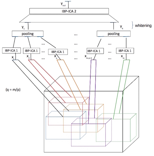
Figure 1: The proposed SC-IBP-ICA architecture. It is trained by using some randomly selected video patches, from each of which we extract an input vector $\boldsymbol{x}$. Pooling is performed between the first and the second layer over small neighborhoods comprising $p$ adjacent first layer units. The outputs of the first layer are presented as inputs to the second layer (after whitening).

3.2 Stacked Convolutional IBP-ICA Networks

Let us now turn to the problem of action recognition in video sequences. Since videos are sequences of images (frames), to address this task using our model we simply extract the component frames of the video sequences at hand and flatten them into a vector, which is eventually presented to our model as the observed input. However, a problem with this model setup is the resulting extremely high dimensionality of the input observations, which induces an excessive increase to the number of inferred model parameters, and, hence, the computational complexity of the inference algorithm of our model.

To alleviate this computational burden, we opt for resorting to a stacked convolutional IBP-ICA network architecture, inspired from local receptive field networks (e.g., [18, 20]). Specifically, instead of processing the whole video frames using a single IBP-ICA model, we use multiple convolved copies of an IBP-ICA model to process smaller (overlapping) patches of the video frame sequences. This way, we manage to dramatically reduce the number of inferred model parameters, and, hence, the imposed computational complexity. The output feature vectors of the postulated component IBP-ICA models are further processed by a pooling sublayer, similar to conventional convolutional neural network architectures. The introduction of pooling into our convolutional IBP-ICA network endows it with the merit of translational invariance, which is a desideratum in the context of action recognition applications in video sequences. Finally, we stack multiple layers of our convolutional IBP-ICA network to obtain a deep learning architecture. Our deep architecture allows for capturing features that correspond to both lower and higher level analysis of the spatiotemporal dynamics in the observed data; this way, it extracts much richer information to train a classifier with, compared to shallow models [1] .

Training of our proposed SC-IBP-ICA network proceeds as follows: Initially, we train an IBP-ICA model on small video patches. Subsequently, we build a convolutional network of IBP-ICA models, by replicating and applying copies of the learned IBP-CA model to different overlapping patches of the input video frame sequences (with an additional pooling sublayer on top). Finally, we feed the output of our convolutional IBP-ICA network to a similarly trained subsequent convolutional IBP-ICA network, thus creating a deep learning architecture through stacking. As a final note, we underline that training of a whole SC-IBP-ICA network is performed in a greedy layerwise manner, similar to many existing convolutional deep learning architectures (e.g., [20]).

A graphical illustration of the proposed SC-IBP-ICA network and its training procedures is provided in Fig. 1.

3.3 Feature Generation Using SC-IBP-ICA

Given a learned SC-IBP-ICA network, feature generation from observed video frame sequences is performed similar to conventional deep convolutional networks, by means of feedforward computation. Specifically, based on the expression of the variational posterior $q(y_{nk})$ derived in Eq. (28), to perform feature generation we feedforward the input vectors $\boldsymbol{x}_{n}$ by application of Eq. (30), using the already obtained values of $\mathbb{E}_{q(\phi)}[\phi]$, $\mathbb{E}_{q(\boldsymbol{G})}[\boldsymbol{G}_{:,k}^{T}\boldsymbol{G}_{:,k}]$, and $\mathbb{E}_{q(\boldsymbol{G})}[\boldsymbol{G}_{:,k}^{T}]$. Note that, from the simple feedforward computation form of Eq. (30), it directly follows that using our method to generate features is extremely fast, with costs identical to existing state-of-the-art approaches, e.g. [18].

Table 1: Mean average precision on the Hollywood2 dataset.

Algorithm	Average Precision
Harris3D + HOG/HOF [36]	45.2%
Hessian + ESURF [36]	38.2%
Cuboids + HOG/HOF [36]	46.2%
convGRBM [30]	46.6%
Dense + HOG3D [36]	45.3%
ISA (with reconstruction	54.6%
penalty) [17]
SC-IBP-ICA (1 layer)	47.8% (286)
SC-IBP-ICA (2 layers)	53.5% (286 - 198)

Table 2: Average accuracy on the YouTube dataset.

Algorithm	Accuracy
HAR + HES	71.2%
+ MSER + SIFT [21]
Harris3D + Grads.	71.2%
+ PCA + Heuristics [21]
ISA [18]	75.8%
SC-IBP-ICA (1 layer)	73.6% (291.7)
SC-IBP-ICA (2 layers)	75.4% (291.7 - 197.9)

Table 3: Average accuracy on the KTH dataset.

Algorithm	Accuracy
Harris3D + HOG/HOF [36]	91.8%
Hessian + ESURF [36]	81.4%
Cuboids + HOG3D [36]	90.0%
HMAX [11]	91.7%
3D-CNN [12]	90.2%
convGRBM [30]	90.0%
ISA [18]	93.9%
SC-IBP-ICA (1 layer)	92.3% (293)
SC-IBP-ICA (2 layers)	93.4% (293 - 195)

Table 4: Average feature extraction time in our experiments (Hollywood2 dataset).

Algorithm	Seconds/Frame
HOG3D	0.20
ISA [18] (1 layer)	0.13
ISA [18] (2 layers)	0.40
SC-IBP-ICA (1 layer)	0.12
SC-IBP-ICA (2 layers)	0.38

4 Experiments

In this section, we experimentally investigate how SC-IBP-ICA compares to the current state-of-the-art in action recognition. To perform our experimental investigations, we use three publicly available action recognition benchmarks, namely Hollywood2 [22], KTH actions, and YouTube actions [21]. Our experimental setup is the same as in [18, 17], adopting exacty the same data preprocessing/postprocessing steps. After extracting local features by means of SC-IBP-ICA, we subsequently perform vector quantization of the obtained feature vectors using K-means. Finally, we use these discretized feature vectors to train an SVM classifier [32] employing a $\chi^{2}$ kernel.

We adopt the same dataset splits and evaluation metrics as in [36, 21]. Specifically, Hollywood2 human actions dataset contains 823 train and 872 test video clips organized into 12 action classes; each video clip may have more than one action label. We utilize the produced feature vectors to train 12 binary SVM classifiers, one for each action. We use the final average precision (AP) metric for our evaluations, computed as the average of AP for each classifier run on the test set. Youtube actions dataset contains 1600 video clips organized into 11 action classes. These video clips have been split into 25 folds which we use to perform 25-fold cross-validation. Note that, from each split, we use only videos indexed 01 to 04, except for the biking and walking classes, where we use the whole datasets. Finally, KTH actions dataset contains 2391 video samples organized into 6 action classes. We split these samples into a test set containing subjects 2, 3, 5, 6, 7, 8, 9, 10, 12, and a training set containing the rest of the subjects. We use the produced feature vectors to train a multi-class SVM.

We evaluate SC-IBP-ICA architectures comprising one and two layers, to examine how extra layer addition affects model performance. Regarding selection of the size of receptive fields of our model, the first layer is of size 16$\times$16 (spatial) and 10 (temporal), while the second one is of size 20$\times$20 (spatial) and 14 (temporal), similar to [18, 36]. The size of the output of the pooling layers is identical to the size of the output of the IBP-ICA models that feed it, i.e. the number of latent features our method discovers. Training is performed on 200,000 video blocks, randomly sampled from the training set of each dataset. We perform dense sampling with 50% overlap in all dimensions. In cases of 2-layer architectures, we train the used SVM classifiers by combining the features generated from both layers. This setup retains more representative features compared to using only the features from the top layer, corresponding to a coarse-to-fine analysis of the observations [20].

Our obtained results are provided in Tables 1-3. Note that the performances of the competing methods reported therein have been cited from [18] and [17]. The reported results of ISA were obtained with 300 latent features on the first layer, and 200 latent features on the second layer (these have been heuristically found to yield the best performance among a large set of evaluated alternatives).

In Tables 1-3, we also provide the number of latent features automatically discovered by our method (in parentheses, beside the accuracy figures). Note that the reported performance results and the corresponding numbers of discovered latent features pertaining to the YouTube dataset, illustrated in Table 2, are means over the 25 splits of the dataset into training and test sets (folds) provided by its creators. We observe that our method obtains performance similar to the state-of-the-art, while also allowing for automatic inference of the appropriate number of generated features. We also observe that addition of a second layer is auspicious in all cases, corroborating similar findings in the literature.

In Table 4, we depict the computational costs of our approach regarding feature extraction from the Hollywood2 (test) dataset (run as a single thread). It is clear that feature generation using our method takes time similar to existing ICA-based approaches, namely the ISA method presented in [18], as theoretically expected (the small computational advantage of our method is presumably due to the lower number of latent features compared to [18]).

Further, we examine model generalization performance under a transfer learning setting: In real-world settings, a feature extraction system pre-trained on samples from a set of video sequences will be expected to perform well on any previously unseen input video sequence, with no samples of it included in its training set. To perform this kind of evaluations, we train our SC-IBP-ICA network on video blocks randomly sampled from the KTH dataset, and evaluate its performance on the Hollywood2 dataset. Under this setup, our method yields a mean average precision equal to 51.9%. Compare this result to the performance obtained by ISA [18] under the same experimental setup, which yields a mean average precision equal to 50.8%.

Finally, an interesting question concerns how IBP-ICA model performance changes in case we use cross-validation to perform model selection instead of sampling from the related posteriors over the number of features [Eqs. (15)-(22)]. To investigate this, we repeat our experiments using the Hollywood2 dataset in the following way: We perform model training without sampling the number of features, which is considered a given constant. We repeat this experiment multiple times, with different numbers of features each time; we try configurations comprising 250-350 features on the first layer, and 150-250 features on the second layer, with a step of 5 features between consecutive evaluated models. Model selection is performed on the grounds of the accuracy obtained in the available test set.

Our findings are illustrated in Table 5; as we observe, cross-validation yields a slightly better model performance than our fully-fledged nonparametric Bayesian approach. However, these mediocre gains come at the price of significant computational costs: Specifically, the computational gain from skipping the updates of the posterior over the number of latent features constitutes only a meager 16.2% of the total training time. On the other hand, the aforementioned cross-validation procedure required evaluating 40 different model configurations, i.e. repeating model training 40 times. Therefore, model selection by means of our nonparametric Bayesian approach offers an overwhelmingly favorable complexity/accuracy trade-off compared to an exhaustive cross-validation technique.

In the same vein, another interesting question concerns comparison of the proposed hybrid variational inference algorithm of our model with the straightforward alternative of Markov chain Monte-Carlo (MCMC) inference. To examine this aspect, we rerun our experiments by properly adapting the MCMC algorithm outlined in [16] in the context of our model. As we observed, our proposed algorithm requires one order of magnitude less time to converge, for a negligible performance deterioration compared to MCMC.

Table 5: Mean average precision on the Hollywood2 dataset by application of cross-validation.

Algorithm	Average Precision	Model Size
SC-IBP-ICA (1 layer)	48.1%	295
SC-IBP-ICA (2 layers)	53.9%	295-205

5 Conclusions

In this paper, we introduced a deep convolutional nonparametric Bayesian approach for unsupervised feature extraction. The main building block of our approach is a nonparametric Bayesian formulation of ICA, dubbed IBP-ICA. Our method imposes a spike-and-slab prior over the factor loadings matrices, driven by an IBP prior over the latent feature activity indicators. This way, it allows for automatic data-driven inference of the most appropriate number of latent features. This is in stark contrast with all existing methods, such as DBNs [9], ICA variants [18, 17], and SAEs [1], where hand-tuning the number of extracted latent features is an essential part of the application of these methods to real-life tasks. It is also substantially different from the related approach of [4], where, instead of the spike-and-slab prior used in this work, a simpler Beta-Bernoulli process prior is employed; this formulation of [4] does not allow for performing feature generation via simple feedforward computation [in the sense of Eq. (30)]. Hence, feature generation in [4] requires much higher computational costs compared to state-of-the-art deep learning approaches and our method. In addition, our approach can model latent feature distributions of arbitrary complexity (approximated via mixtures of Gaussians, Eq. (2)), as opposed to [4] which postulates a simplistic spherical Gaussian prior.

We devised an efficient variational inference algorithm for our model. Our method is very easy to train because (batch) variational inference does not need any tweaking with heuristics such learning rates and convergence criteria. In this regard, our method lies on exactly the opposite side of the spectrum compared to conventional approaches based on neural networks: Our method entails no need of selection of training algorithm heuristics, whatsoever, while training neural networks is a tedious procedure requiring a great deal of hand-tuning of several heuristics (e.g., learning rate, weight decay, convergence parameters, inertia).

We evaluated our approach using three well-known action recognition benchmarks, adopting a standard video processing pipeline (e.g., [31]). As we showed, our method yields results similar to the state-of-the-art for these benchmarks, while imposing competitive computational costs for feature generation. These results corroborate that nonparametric Bayesian models can offer a viable alternative to existing deep feature extractors, and at the same time mitigate some of the major hurdles deep nets are confronted with, regarding data-driven selection of model size during inference, and learning algorithm parameters fine-tuning.

Appendix

We have

$$q(\lambda_{k})=\mathcal{G}(\lambda_{k}|\tilde{c}_{k},\tilde{f}_{k})$$ (37)

where

$$\tilde{c}_{k}=c+\frac{1}{2}\sum_{d=1}^{D}q(z_{dk}=1),\;\;\tilde{f}_{k}=f+\sum_{d=1}^{D}\mathbb{E}_{q(g_{dk})}[g_{dk}^{2}]$$ (38)

and

$$q(\phi)=\mathcal{G}\big{(}\phi\big{|}a+\frac{ND}{2},b+ \sum_{n=1}^{N}(\boldsymbol{x}_{n}-\mathbb{E}_{q(\boldsymbol{y}_{n}),q(\boldsymbol{G})}[\boldsymbol{G}\boldsymbol{y}_{n}])^{T}$$ (39)

$$\times(\boldsymbol{x}_{n}-\mathbb{E}_{q(\boldsymbol{y}_{n}),q(\boldsymbol{G})}[\boldsymbol{G}\boldsymbol{y}_{n}])\big{)}$$

For the stick-variables $v_{k}$, we adopt the approximations [6]:

$$q(v_{k})=\mathrm{Beta}(v_{k}|\tilde{\tau}_{k},\hat{\tau}_{k})$$ (40)

$$\tilde{\tau}_{k}= \sum_{m=k+1}^{K}\left(D-\sum_{d=1}^{D}q(z_{dm}=1)\right)\sum_{i=k+1}^{m}q_{i}$$ (41)

$$+\sum_{d=1}^{D}\sum_{m=k}^{K}q(z_{dm}=1)+\mathbb{E}_{q(\alpha)}[\alpha]$$

$$\hat{\tau}_{k}=1+\sum_{m=k}^{K}\left(D-\sum_{d=1}^{D}q(z_{dm}=1)\right)q_{k}$$ (42)

where we denote $K\triangleq\underset{d}{\mathrm{max}}\;K_{d}$,

$$q_{k}\propto\mathrm{exp} \big{(}\psi(\hat{\tau}_{k})+\sum_{i=1}^{k-1}\psi(\tilde{\tau}_{i})-\sum_{i=1}^{k}\psi(\tilde{\tau}_{i}+\hat{\tau}_{i})\big{)}$$ (43)

and $\psi(\cdot)$ is the Digamma function. Finally, the innovation hyperparameter yields: $q(\alpha)=\mathcal{G}(\alpha|\tilde{\gamma}_{1},\tilde{\gamma}_{2})$, where $\tilde{\gamma}_{1}=\gamma_{1}+K-1$ and $\tilde{\gamma}_{2}=\gamma_{2}-\sum_{k=1}^{K-1}[\psi(\tilde{\tau}_{k})-\psi(\tilde{\tau}_{k}+\hat{\tau}_{k})]$.

References

- [1] Y. Bengio, P. L. D. Popovici, and H. Larochelle. Greedy layerwise training of deep networks. In Proc. NIPS, 2006.
- [2] C. M. Bishop. Pattern Recognition and Machine Learning. Springer, New York, 2006.
- [3] S. Chatzis, D. Kosmopoulos, and T. Varvarigou. Signal modeling and classification using a robust latent space model based on distributions. IEEE Trans. Signal Processing, 56(3):949–963, March 2008.
- [4] B. Chen, G. Polatkan, G. Sapiro, D. B. Dunson, and L. Carin. The hierarchical Beta process for convolutional factor analysis and deep learning. In Proc. ICML, 2011.
- [5] P. Dollar, V. Rabaud, G. Cottrell, and S. Belongie. Behavior recognition via sparse spatio-temporal features. In Proc. ICCN, pages 65–72, Washington, DC, USA, 2005.
- [6] F. Doshi-Velez, K. Miller, J. V. Gael, and Y. W. Teh. Variational inference for the Indian buffet process. In Proc. AISTATS, 2009.
- [7] D. Erhan, C. Szegedy, A. Toshev, and D. Anguelov. Scalable object detection using deep neural networks. In Proc. CVPR, pages 2155 – 2162, 2014.
- [8] T. L. Griffiths and Z. Ghahramani. Infinite latent feature models and the Indian buffet process. In Proc. NIPS, 2006.
- [9] G. Hinton, S. Osindero, and Y. Teh. A fast learning algorithm for deep belief nets. Neu. Comp., 2006.
- [10] A. Hyvarinen, J. Hurri, and P. Hoyer. Natural Image Statistics. Springer, 2009.
- [11] H. Jhuang, T. Serre, L. Wolf, and T. Poggio. A biologically inspired system for action recognition. In Proc. ICCV, 2007.
- [12] S. Ji, W. Xu, M. Yang, and K. Yu. 3D convolutional neural networks for human action recognition. In Proc. ICML, 2010.
- [13] M. Jordan, Z. Ghahramani, T. Jaakkola, and L. Saul. An introduction to variational methods for graphical models. In M. Jordan, editor, Learning in Graphical Models, pages 105–162. Kluwer, Dordrecht, 1998.
- [14] A. Karpathy, G. Toderici, S. Shetty, T. Leung, R. Sukthankar, and L. Fei-Fei. Large-scale video classification with convolutional neural networks. In Proc. CVPR, pages 1725–1732, 2014.
- [15] A. Kläser, M. Marszałek, and C. Schmid. A spatio-temporal descriptor based on 3d-gradients. In Proc. BMVC, pages 995–1004, sep 2008.
- [16] D. Knowles and Z. Ghahramani. Nonparametric Bayesian sparse factor models with application to gene expression modeling. Annal. Applied Stat., 5(2B):1534–1552, 2011.
- [17] Q. V. Le, A. Karpenko, J. Ngiam, and A. Y. Ng. ICA with reconstruction cost for efficient overcomplete feature learning. In Proc. NIPS, 2011.
- [18] Q. V. Le, W. Y. Zou, S. Y. Yeung, and A. Y. Ng. Learning hierarchical invariant spatio-temporal features for action recognition with independent subspace analysis. In Proc. CVPR, 2011.
- [19] H. Lee, A. Battle, R. Raina, and A. Y. Ng. Efficient sparse coding algorithms. In Proc. NIPS, 2007.
- [20] H. Lee, R. Grosse, R. Ranganath, and A. Ng. Convolutional deep belief networks for scalable unsupervised learning of hierarchical representations. In Proc. ICML, 2009.
- [21] J. Liu, J. Luo, and M. Shah. Recognizing realistic actions from videos “in the wild”. In Proc. CVPR, 2009.
- [22] M. Marzalek, I. Laptev, and C. Schmid. Actions in context. In Proc. CVPR, 2009.
- [23] E. Meeds, Z. Ghahramani, R. Neal, and S. Roweis. Modeling dyadic data with binary latent factors. In Proc. NIPS, 2006.
- [24] D. Mimno, M. D. Hoffman, and D. M. Blei. Sparse stochastic inference for latent Dirichlet allocation. In Proc. ICML, 2012.
- [25] T. J. Mitchell and J. J. Beauchamp. Bayesian variable selection in linear regression (with discussion). Journal of the American Statistical Association, 83:1023–1036, 1988.
- [26] B. A. Olshausen. Sparse coding of time-varying natural images. In Proc. ICA, 2000.
- [27] M. Oquab, L. Bottou, I. Laptev, and J. Sivic. Learning and transferring mid-level image representations using convolutional neural networks. In Proc. CVPR, pages 1717 – 1724, 2014.
- [28] R. Raina, A. Madhavan, and A. Y. Ng. Large-scale deep unsupervised learning using graphics processors. In Proc. ICML, 2009.
- [29] S. Richardson and P. Green. On Bayesian analysis of mixtures with unknown number of components. J. Roy. Statist. Soc. B, 59:731–792, 1997.
- [30] G. Taylor, R. Fergus, Y. Lecun, and C. Bregler. Convolutional learning of spatio-temporal features. In Proc. ECCV, 2010.
- [31] J. van Hateren and D. Ruderman. Independent component analysis of natural image sequences yields spatio-temporal filters similar to simple cells in primary visual cortex. Proceedings of the Royal Society: Biological Sciences, 1998.
- [32] V. N. Vapnik. Statistical Learning Theory. Wiley, New York, 1998.
- [33] P. Vincent, H. Larochelle, I. Lajoie, Y. Bengio, and P.-A. Manzagol. Stacked denoising autoencoders: Learning useful representations in a deep network with a local denoising criterion. J. Machine Learning Research, 11:3371–3408, 2010.
- [34] H. Wang, A. Klaser, C. Schmid, and C.-L. Liu. Action recognition by dense trajectories. In Proc. CVPR, pages 3169–3176, 2011.
- [35] H. Wang, M. M. Ullah, A. Klaser, I. Laptev, and C. Schmid. Evaluation of local spatio-temporal features for action recognition. In Proc. BMVC, pages 124.1–124.11, 2009. doi:10.5244/C.23.124.
- [36] H. Wang, M. M. Ullah, A. Klaser, I. Laptev, and C. Schmid. Evaluation of local spatio-temporal features for action recognition. In Proc. BMVC, 2010.
- [37] G. Willems, T. Tuytelaars, and L. Gool. An efficient dense and scale-invariant spatio-temporal interest point detector. In Proc. ECCV, pages 650–663, 2008.