Percolation of the Site Random-Cluster Model by Monte Carlo Method

Abstract

We propose a site random cluster model by introducing an additional cluster weight in the partition function of the traditional site percolation. To simulate the model on a square lattice, we combine the color-assignation and the Swendsen-Wang methods to design a highly efficient cluster algorithm with a small critical slowing-down phenomenon. To verify whether or not it is consistent with the bond random cluster model, we measure several quantities such as the wrapping probability $R_{e}$, the percolating cluster density $P_{\infty}$, and the magnetic susceptibility per site $\chi_{p}$ as well as two exponents such as the thermal exponent $y_{t}$ and the fractal dimension $y_{h}$ of the largest percolating cluster. We find that for different exponents of cluster weight $q=1.5$, $2$, $2.5$, $3$, $3.5$ and $4$, the numerical estimation of the exponents $y_{t}$ and $y_{h}$ are consistent with the theoretical values. The universalities of the site random cluster model and the bond random cluster model are completely identical. For larger values of $q$, we find obvious signatures of the first-order percolation transition by the histograms and the hysteresis loops of percolating cluster density and the energy per site. Our results are helpful for the understanding of the percolation of traditional statistical models.

I Introduction

Broadbent and Hammersley initially presented the concept of percolationbroad ; hamer ; Grimmett , and then Stauffer introduced the properties of percolation in detailstauffer . There have been broad applications of percolation: e.g. fluids in porous mediumpos , the spread of infectious diseases on complex networksdis , the Hall effect with quantum spin hall , network vulnerabilityneta ; netb , forest firesfire , number theoryvardi , etc $\ldots$

The most studied percolation models are percolations on regular lattices, in which a site (bond) on the lattice could be occupied (vacant) with probability $p$ (or $1-p$). At a given critical probability $p_{c}$, at least one large cluster, formed by the occupied sites (bonds), spans to the opposite boundaries in the latticesbroad ; hamer ; Grimmett .

The construction of a site percolation or bond percolation is similar. However, they are independent in some respects. For example, the site percolation transition on the square lattice occurs at $p_{c}=0.59274621(13)$ according to the high precision Monte Carlo methodziff1 , while, the exact solution indicates that the bond percolation transition point $p_{c}=\frac{1}{2}$ on the square latticebondperco . In the Monte Carlo simulations near $p_{c}$, the configurations are completely disordered and the local structures in the configurations vary in a significant random fashionmonte .

The invariances behind the configurations are the critical exponents and the universalities, which are the same for the two types of percolations, without consideration of the site, the bond, or other microscopic detailsuniversal .

Universality connects the phase transitions in a number of lattice statistical models to the percolation transition. One important model, the bond random cluster (BRC) modelrcm created by Fortuin and KasteleynPWK in the 1960s, gives us a unified description of several classical statistical models, including the Ising, PottsFYW , Ashkin-Tellerashkinteller and the percolation models. This body of work results in the extensions of the BRC model and many new possible critical behaviorstri ; guo1 ; deng2 .

An additional cluster weight factor in the partition function is the significant difference between the bond percolation model and the BRC model. Inspired by this, we propose a new model, the site RC (SRC) model which is made by combining the site percolation and the RC model, and adding a cluster weight factor in the partition function.

To investigate the critical behaviors of the new SRC model, we design a cluster-updating Monte Carlo method and simulate the new model. Many useful quantities are measured, such as the wrapping probability $R_{e}$, the percolating cluster density $P_{\infty}$ and the magnetic susceptibility per site $\chi_{p}$. By performing finite size scaling analysis of the above quantities, the very precise phase transition points are obtained. We also calculate the thermal exponent $y_{t}$, and the fractal dimension $y_{h}$ of the largest percolating cluster in such a way as to check that whether or not the universalities of the BRC percolation and the SRC percolation are completely consistent.

The outline of this work is as follows. Sec. II shows a brief review of the BRC model and shows how we generalize the site percolation model to the SRC model. Sec. III describes the algorithm and several sampled quantities in our Monte Carlo simulations. Numerical results are then presented in Sec. IV. Conclusive comments are made in Sec. V.

II Model

II.1 Potts Model and BRC model

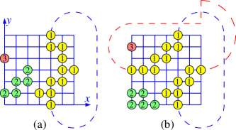
Figure 1: (a) A typical configuration of a SRC model on a two dimensional lattice with size $L=7$, in which the number of clusters $n_{c}$ is 3 and the number of the occupied sites $n_{s}$ is $17$. The two circles labeled by “$1$” in the top and bottom collected by the dashed line, which means the first cluster is a wrapping cluster. (b) A cluster labeled by ’1’, distributed diagonally or ”spirally”ziff1 , wraps around both directions before joining up.

This section provides a brief review of two classical models in statistical physics: the Potts modelFYW and its generalization to the BRC modelPWK . The reduced Hamiltonian of the Potts model is:

$$\beta H=-K\sum_{\langle{ij}\rangle}\delta_{{\sigma}_{i},{\sigma}_{j}},$$ (1)

where ${\langle{ij}\rangle}$ means the nearest-neighbor summation, $K$ is the coupling interaction, $\beta$ is the inverse temperature, $\sigma_{i}$ is the state variable on the site $i$ and can be any natural number less than or equal to $q$. If $q=2$, the model is identical to the Ising model without an external field, which has two states for each spin. The partition function of the Potts model is:

$$Z =\sum_{\sigma}\prod_{\langle ij\rangle}e^{K\delta_{\sigma_{i},\sigma_{j}}}$$ (2)

$$=\sum_{\sigma}\prod_{\langle ij\rangle}(1+u\delta_{\sigma_{i},\sigma_{j}})~{},$$

where the symbol $u$ is the bond weight and defined as $u=e^{K}-1$sh . The above equation can be transformed into:

$$Z =\sum_{\sigma}\prod_{\langle ij\rangle}\sum_{b_{ij}=0}^{1}(u\delta_{\sigma_{i},\sigma_{j}})^{b_{ij}}$$ (3)

$$=\sum_{\{b\}}\sum_{\sigma}\prod_{\langle ij\rangle}(u\delta_{\sigma_{i},\sigma_{j}})^{b_{ij}}~{},$$

where the bond variable $b_{ij}=0$ if $\sigma_{i}\neq\sigma_{j}$ while $b_{ij}=1$ if $\sigma_{i}=\sigma_{j}$. Through the summation over the spin variable $\sigma$, the partition function Eq. (3) becomes

$$Z_{\text{BRC}}=\sum_{\{b\}}u^{n_{b}}q^{n_{c}}~{},$$ (4)

where the sum is over all bond configurations $\{b\}$, $n_{b}=\sum b_{ij}$ is the bond number in the configurations, and $n_{c}$ is the number of clusters. The discrete number $q$ now appears as a continuous variable. Thus, the BRC model can be regarded as a generalization of the Potts model. In the limit $q\to 1$, it reduces to the bond-percolation model, whose partition function is:

$$Z=\sum_{\{b\}}(e^{K}-1)^{n_{b}}$$ (5)

This form can be easily transformed into:

$$Z=\sum_{\{b\}}p^{n_{b}}_{b}(1-p_{b})^{N_{b}-n_{b}}$$ (6)

where $p_{b}=\frac{u}{1+u}$ and $N_{b}$ is the total number of bonds in the lattice. The significant difference between the partition functions of the bond percolation model and the RC model is that Eq. (4) has the cluster weight $q^{n_{c}}$ while Eq. (6) does not.

II.2 SRC model

Now, we generalize the site percolation to the SRC modelrcm . The partition function of the site percolation is:

$$Z=\sum_{\{\sigma\}}p^{n_{s}}_{s}(1-p_{s})^{N-n_{s}},$$ (7)

where $N=L\times L$ is the total number of sites. We directly generalize it by introducing a cluster weight $q^{n_{c}}$, and then derive the partition function of the SRC model as:

$$Z_{\text{SRC}} =\sum_{\{\sigma\}}p^{n_{s}}_{s}(1-p_{s})^{N-n_{s}}q^{n_{c}}$$ (8)

$$\propto\sum_{\{\sigma\}}u^{n_{s}}q^{n_{c}}$$

where $p_{s}=\frac{u}{1+u}$, $n_{s}$ is the number of occupied sites, $N-n_{s}$ is the number of vacant sites, and $p_{s}$ is the occupation probability for the sites in the configuration. The weight of a configuration is given by:

$$W=p_{s}^{n_{s}}(1-p_{s})^{N-n_{s}}q^{n_{c}}$$ (9)

As shown in Fig. 1, the weight of the typical configuration is $p_{s}^{17}(1-p_{s})^{32}q^{3}$.

III algorithm and the Sampled Quantities

III.1 algorithm

There are a few efficient methodsmd1 to simulate the RC model. In the present paper, we combine the color-assignationcolor1 ; color2 and the Swendsen-Wangswendsen methods together to design a highly efficient cluster algorithm with a small critical slowing-down phenomenon. Similar methods have been applied in several papersding1 ; ding2 . The algorithm to simulate this model is as follows:

1. Initially, all sites are active.

2. Active sites are randomly assigned to be occupied, with probability $p$ or vacant with probability $1-p$. After all sites have been assigned, they are grouped into clusters: if nearest neighbor sites are both occupied, they belong to the same cluster. Vacant sites don’t belong to any cluster.

3. With probability $1-\frac{1}{q}$, clusters are declared inactive. The boundary sites-the nearest neighbors of the sites belonging to an inactive occupied cluster-are also inactive. All other sites are declared active, in effect erasing their contents.

4. If there are any active sites, return to step 2. Otherwise, we have constructed a configuration that obeys the statistics of Eq. (9).

We define the percolation cluster as follows: If any cluster spans the whole lattice, the configuration is called a percolation configuration. For a finite system, it can be defined by various rules. In the present work, a percolation state means there is at least one “wrapping” clusterwrap in the lattice and ”wrapping” refers to a cluster that connects itself along one of the lattice directions. For example, in Fig. 1 (a), the cluster labeled by ”1” is a wrapping cluster, and the wrapping direction is the vertical direction. The wrapping cluster is only applicable to a lattice with periodic boundary conditions.

In Fig. 1 (b), the occupied sites labeled by ’1’ are distributed diagonally or ”spirally” in the lattice. In this case, the cluster wraps around both horizontal and vertical directions, which is called the “single spiral” configurationziff1 .

III.2 the sampled quantities

In order to obtain the critical phase transition points, we define the wrapping probability as:

$$R_{e}=\langle R_{x}+R_{y}\rangle/2,$$ (10)

where the subscript $e$ represents a cluster forming along the $x$ or $y$ direction, and $\langle\dots\rangle$ denotes ensemble averaging. If a wrapping cluster exists in the $x$ direction, then $R_{x}=1$, otherwise, $R_{x}=0$. The rule is the same for the $y$ direction. If a cluster forming along both $x$ and $y$ direction, then both $R_{x}=1$ and $R_{y}=1$.

The SRC model can be explored in view of site percolation. Therefore, we can define the order parameter of the percolating cluster density and magnetic susceptibility per site :

$$P_{\infty}=\langle P\rangle=L^{-d}\langle n_{\infty}\rangle$$ (11)

$$\chi_{p}=L^{-2d}\langle\sum_{i=1}^{n_{c}}n_{i}^{2}\rangle$$ (12)

where $n_{\infty}$ is the size (the number of sites) of the percolating cluster and $d=2$ is dimensionality of the lattice. According to the finite-size scaling theorynight ; baxter , the above parameters provide us the scaling behavior of them as a function of the system size $L$ and the site occupation probability $p$:

$$\begin{split}R_{e}&=R_{e}^{(0)}+a_{1}(p-p_{c})L^{y_{t}}+a_{2}(p-p_{c})^{2}L^{2y_{t}}+\cdots\\ &+b_{1}L^{y_{1}}+b_{2}L^{y_{2}}+\cdots~{}.\end{split}$$ (13)

$$P_{\infty}=L^{y_{h}-d}(e_{0}+e_{1}(p-p_{c})L^{y_{t}}+e_{2}(p-p_{c})^{2}L^{2y_{t}}+\cdots$$

$$~{}~{}\qquad\qquad+f_{1}L^{y_{1}}+f_{2}L^{y_{2}}+\cdots)$$ (14)

$$\chi_{p}=L^{2y_{h}-2d}(g_{0}+g_{1}(p-p_{c})L^{y_{t}}+g_{2}(p-p_{c})^{2}L^{2y_{t}}+\cdots$$

$$~{}~{}\qquad\qquad+h_{1}L^{y_{1}}+h_{2}L^{y_{2}}+\cdots)$$ (15)

It should be noted that the occupation probability is for the site occupation, instead of the bond occupation probabilitybon , where $p_{c}$ is the percolation threshold, $y_{t}$ is the thermal exponent, $y_{h}$ is the fractal dimension of the percolating cluster, $d$ is the space dimension, and $y_{1}$, $y_{2}$, $\cdots$, are negative correction-to-scaling exponents.

Eqs. (13)-(15) give a model scaling form for various physical quantities. The three quantities $R_{e}$, $P_{\infty}$ and $\chi_{p}$ are assumed in an analytic function in $p$ and $L$ at the percolation critical point, so that it has a series expansion here. These analytic functions, will be used as a basis for fitting the numerical data. The three scaling functions that are being expanded depend on the same scaling variables, but they are, in general, distinct functions. Hence, when expanded, the expansion coefficients $a_{i}$, $b_{i}$, $e_{i}$, $f_{i}$, $g_{i}$, $h_{i}$ ($i=1,2,\cdots$) will, in general, be different. Therefore we use different symbols to denote them.

III.3 fitting at the critical points

The fitting functions in Eqs. (14) and (15), the quantities $P_{\infty}$ and $\chi_{p}$, depend on the expansion coefficients. So it is necessary to deduce the value of $P_{\infty}$ and $\chi_{p}$. At the percolation point $p_{c}$, Eqs. (14) and (15) reduce to:

$$P_{\infty} =L^{y_{h}-d}(e_{0}+f_{1}L^{y_{1}}+f_{2}L^{y_{2}}+\cdots)$$ (16a)

$$\chi_{p} =L^{2y_{h}-2d}(g_{0}+h_{1}L^{y_{1}}+h_{2}L^{y_{2}}+\cdots),$$ (16b)

which will be used to determine the exponent $y_{h}$.

To see more readily the importance of the corrections to scaling, we divide out the leading dependence on $L$ in Eqs. (16a) and (16b) just using the first two terms. Fitting data according to

$$L^{d-y_{h}}P_{\infty} =e_{0}+f_{1}L^{y_{1}}$$ (17a)

$$L^{2d-2y_{h}}\chi_{p} =g_{0}+h_{1}L^{y_{1}}$$ (17b)

will help see clearly the corrections to the scaling terms.

IV Results

Firstly, we do a Monte Carlo simulation of the SRC model on the square lattice with the above algorithm. We find the algorithm has a small critical slowing-down phenomena with $q\leq 4$ and consequently we sample between every two Monte-Carlo steps. As the system enters into equilibrium states, we take $10^{8}$ samples to calculate each quantity for the system sizes $8\leq L\leq 64$, and we take $10^{7}$ samples for the system sizes $128\leq L\leq 256$FDB .

To obtain the critical point $p_{c}$, and the exponent $y_{t}$, we perform a finite-size scaling analysis of the wrapping probability $R_{e}$ for various system sizes near the critical occupation probability $p_{c}$. At the critical point $p_{c}$, we calculate the percolating cluster density $P_{\infty}$ and the magnetic susceptibility per site $\chi_{p}$ to obtain the exponent $y_{h}$. We also study the cases for larger values of $q$, such as $q=10$ and find a interesting first-order phase transition.

IV.1 Theoretical and numerical exponents $y_{t}$ and $y_{h}$ for q=1.5-4

The theoretical values of the exponents $y_{t}$ and $y_{h}$ can be obtained by the Coulomb gas methodcoulomb or conformal invarianceconformal , and they are given by:

$$\sqrt{q} =-2~{}\cos(\pi g),$$ (18a)

$$y_{t} =3-\frac{3}{2g},$$ (18b)

$$y_{h} =1+\frac{g}{2}+\frac{3}{8g}.$$ (18c)

where the coupling constant $g$ of the Coulomb gas is in the range $1/2\leq g\leq 1$. According to the above equations, the theoretical values of the both exponents will be shown in the following section.

The numerical results by Monte Carlo method are listed in table 1. For $q=1.5,~{}2,~{}2.5,~{}3,~{}3.5$ and $4$, the percolation threshold $p_{c}$, the wrapping probability $R_{e}$, the thermal exponent $y_{t}$, and the fractal dimension of the percolation cluster $y_{h}$ are obtained in the same way, which will be discussed in detail next subsections. We find that for the range $q=1.5-3$, the numerical results $y_{h}$ and $y_{t}$ are very consistent with the theoretical values. For $q=3.5$ and $4$, the precision of the critical point and the exponents are lower than the case with other values of $q$, due to the logarithmic correctionlog1 ; log2 ; log3 .

Table 1: Numerical results(N) for the percolation threshold $p_{c}$, the wrapping probability $R_{e}$, the thermal exponent $y_{t}$, and the fractal dimension $y_{h}$ from $\chi_{p}$. Theoretical predictions(T) are included where available by the Coulomb gas methodcoulomb or conformal invarianceconformal . The estimated errors in the last decimal place are shown between parentheses.

q		$p_{c}$	$R_{e}$	$y_{t}$	$y_{h}\leftarrow\chi_{p}$
1.5	N	0.726525(2)	0.5822(3)	0.884(4)	1.8831(7)
	T	–	–	0.887	1.8832
2	N	0.805000(1)	0.6270(1)	1.000(5)	1.8750(5)
	T	–	–	1.000	1.8750
2.5	N	0.854411(2)	0.6637(3)	1.101(7)	1.8698(4)
	T	–	–	1.102	1.8697
3	N	0.887435(1)	0.6955(2)	1.196(5)	1.8664(7)
	T	–	–	1.200	1.8667
3.5	N	0.910600(2)	0.7242(8)	1.311(8)	1.867(1)
	T	–	–	1.305	1.866
4	N	0.927476(1)	0.750(1)	1.44(7)	1.88(1)
	T	–	–	1.50	1.88

IV.2 $q=1.5$, detailed analysis

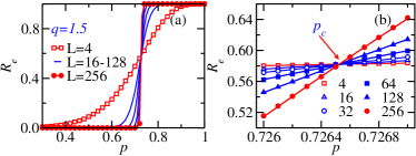
Figure 2: Wrapping probability $R_{e}$ versus site-occupation probability $p$ at $q=1.5$ in the ranges (a) $0.2<p<1$ and (b) $0.7260<p<0.7272$, with different sizes $L=4,~{}8,~{}16,~{}32,~{}64,~{}128$, and $256$. The critical point is $p_{c}=0.726525(2)$ and $R_{e}=0.5822(3)$. The error bars are smaller than the symbols. The lines in the right figure are plotted to guide the reader.

As shown in Fig. 2(a), we calculate the wrapping probability $R_{e}$ as a function of site occupation probability $p$ at $q=1.5$ for lattices with different sizes $L=4,~{}8,~{}16,~{}32,~{}64,~{}128$, and $256$. In the limit $p\rightarrow 0$, no sites are occupied and hence no clusters exist and $R_{e}=0$. In the limit $p\rightarrow 1$, all sites are occupied and a wrapping cluster forms and $R_{e}=1$.

In the region of the critical points, i.e., $0.7260<p<0.7272$, the data looks nearly linear as shown in Fig. 2(b). Using the Levenberg-Marquardt least-squares methodlm and Eq. (13), we find that the critical percolation probability is at $p_{c}=0.726525\text{(}2\text{)}$. Correspondingly, the thermal exponent is $y_{t}=0.884(4)$, which is consistent with the theoretical result $y_{t}=0.887$.

In the fitting procedure, the chi-square

$$\chi^{2}=\sum_{L_{i}}\left(\frac{R_{e}\left(p,L_{i}\right)-R_{e}^{fit}\left(p,L_{i}\right)}{\sigma^{2}_{i}}\right)^{2}$$ (19)

is performedfit1 ; fit2 by summing over the sizes $L=16,32,64,128,256$. The order of magnitude of chi-square is 10. The ratio of chi-square to degree of freedom of fit $\chi^{2}/d.o.f$ is $1.04$, which was thought to be a moderately good fit. $\sigma_{i}$ is the error of $R_{e}$ measured by the Monte Carlo method. $R_{e}^{fit}$ represents the fitting function of $R_{e}$ in Eq. (13). The results with $L=4,8$ are dropped and the higher terms in the expansion are also dropped, i.e., $a_{i}=0,i=3,4,\cdots$ and $b_{i}=0,i=2,3,\cdots$.

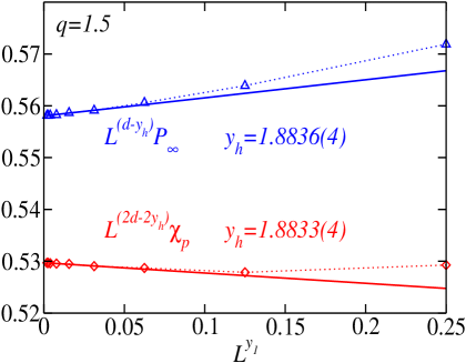
Figure 3: $L^{2d-2y_{h}}\chi_{p}$ and $L^{d-y_{h}}P_{\infty}$ versus $L^{y_{1}}$ of the SRC model for $q=1.5$ on the square lattice with $L=32,64,128,256$ and $512$. The exponent is fixed being $y_{1}=-1$. The two solid lines represent fits to the data points according to Eqs. (17a) and (17b). The fitted exponent $y_{h}$ are 1.8836(4) and 1.8833(4) from $L^{d-y_{h}}P_{\infty}$ and $L^{2d-2y_{h}}\chi_{p}$ , respectively. The dashed lines are plotted to guide the reader.

Figure 3 displays the plot $L^{2d-2y_{h}}\chi_{p}$ and $L^{d-y_{h}}P_{\infty}$ versus $L^{y_{1}}$ at the percolation point. The plot symbols for systems with sizes $L=32-512$ sit in the fitted lines very well, as expected. For small systems with sizes $L=4,8,16$, the plot symbols deviate from the fitted line. Obviously, the correction-to-scaling of $L^{d-y_{h}}P_{\infty}$ is similar with that of $L^{2d-2y_{h}}\chi_{p}$bon . In the real fitting procedure, we neglected the data with sizes $L=4-16$ and the order of magnitude of the residual equals to $10^{-9}$, which means the results are still reliable.

The leading correction-to-scaling exponenty1 is known to be $y_{1}\approx-1$. A least-squares criterion was used to fit the data with $y_{1}$ being fixed at $-1$. By fitting the data of $L^{d-y_{h}}P_{\infty}$, the exponent is fitted and found to be $y_{h}=1.8836(4)$. However, by the fitting of $L^{2d-2y_{h}}\chi_{p}$, the exponent becomes $y_{h}=1.8833(4)$, which is consistent with the result from $P_{\infty}$. The slopes $f_{1}=0.035(7)$ and $h_{1}=-0.020(2)$ for both fitted lines and the first expanded coefficients $e_{0}=0.5580(5)$ and $g_{0}=0.5297(2)$ are also obtained.

For larger systems, the correction terms in Eqs. (17a) and (17b) are far less than the first terms $e_{0}$ and $g_{0}$ at the critical points and therefore the power law $P_{\infty}/\chi_{p}\propto L^{d-y_{h}}$ can be obtained by neglecting the correction terms. In fact, scaling theory for percolation (e.g. see deGennes ; Grimmett ; stauffer ) predicts that phase transitions exhibit scaling properties or “power laws”. Moreover, power laws like Newton’s gravitational law or Coulomb’s law or even Lotka’s law for publication rateslotka are ubiquitous and it is reassuring to recover a power law here as well.

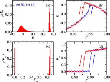
Figure 4: The signature of the first-order phase transition for the SRC model at $q=10$ on a $16\times 16$ square lattice. Histogram of energy per site $E$ (a) and the percolation strength $P_{\infty}$ (c) at the critical point $p_{c}=0.987$. Hysteresis loop of the both quantities $E$ (b) and $P_{\infty}$ (d) around the critical point $p_{c}$.

IV.3 $q=10$, a first-order phase transition

Figure 4 (a) shows a histogram of the energy per site $E$ at the critical point $p_{c}=0.987$, in which the double distribution is a typical signature of the first-order phase transition from the non-percolation phase to the percolation. We obtain the histogram in such a way. Firstly, we initialize a configuration by assigning each site with an occupied or an empty state, a probability of $1/2$. After the system enters into an equilibrium state, we measure the energy per site $E$. We repeat the above steps until the shape of the histogram converges.

To confirm the first-order of the percolation transition, Fig. 4 (b) shows the hysteresis loop around the critical point region, i.e., $0.975<p<1$. The hysteresis loops have been observed both in classicaldeng and quantum systems steep ; hysloop1 ; hysloop2 ; hysloop3 . To form a closed hysteresis loop, we start at $p=0.975$. Then we increase the occupation probability $p$ and sample the energy per site $E$. In the simulation, we use the configuration of the previously completed simulation for a given value of “$p$”, as the (new) initial configuration of the simulation of another value of “$p$”. The energy per site $E$ of the system does not jump to a higher value immediately until $p$ exceeds over a short distance of the transition point $p_{c}$. After $p$ reaches $1$, we decrease $p$ in the same way with regards to the initialization of configurations. A closed hysteresis loop forms when $p$ becomes smaller than $p_{c}$. We repeat similar steps for the $P\infty$ and the results are shown in Figs. 4 (c) and (d).

V Conclusion

In conclusion, we have proposed a new statistical model, which can be considered as a SRC model with an additional cluster weight in the partition function with respect to the traditional site percolation model.

We have also designed a color-assigned cluster updating Monte Carlo simulation algorithm suffering little from the boring critical slowing-down phenomena.

Both of the BRC and SRC percolation models have the same universality by simulations of the SRC model on the square lattice and behaviors of the quantities $R_{e}$, $P_{\infty}$, $\chi_{p}$, $y_{t}$ and $y_{h}$.

At the critical phase transition point the case of $q=1.5$, the correction-to-scaling of $P_{\infty}$ is close to that of $\chi_{p}$. The fitted exponent $y_{h}$ from $P_{\infty}$ has the same precision with that from $\chi_{p}$. For $q=4$, the estimation of exponents $y_{t}$ and $y_{h}$ is less precise due to the log-correction. For $q=10$, the obvious first-order transition is observed.

Our results can be considered as a first study of the counterpart for the BRC percolation model and are helpful for the understanding of the percolation of traditional statistical models.

- (1) S. R. Broadbend and J. M. Hammersley, Proc. Camb. Phil. Soc. 53, 629 (1957).
- (2) J. M. Hammersley, in Percolation Structure and Process, edited by G. Deutscher, R. Zallen and J. Adler (Adam Hilger, Bristol, 1983).
- (3) G. Grimmett, in Percolation (Springer-Verlag, New York, 1989).
- (4) D. Stauffer and A. Aharony, in Introduction to Percolation Theory (Taylor & Francis, Philadelphia, 1994).
- (5) A. Hunt and R. Ewing, in Percolation Theory for Flow in Porous Media (Springer-Verlag, Berlin Heidelberg, 2009).
- (6) M. E. J. Newman, Phys. Rev. E 66, 016128 (2002).
- (7) R. L. Chu, J. Lu, and S. Q. Shen, Europhys. Lett. 100, 17013 (2012).
- (8) R. Cohen, K. Erez, D. Ben-Avraham, and S. Havlin, Phys. Rev. Lett. 85, 4626 (2000).
- (9) D. S. Callaway, M. E. J. Newman, S. H. Strogatz, and D. J. Watts, Phys. Rev. Lett. 85, 5468 (2000).
- (10) P. Bak, K. Chen, and C. Tang, Phys. Lett. A 147, 297 (1990); C. L. Henley, Phys. Rev. Lett. 71, 2741 (1993).
- (11) I. Vardi, Experiment. Math. 7, 275 (1998).
- (12) M. E. J. Newman and R. M. Ziff, Phys. Rev. Lett. 85, 4104 (2000).
- (13) Y. J. Deng and H. W. J. Blöte, Phys. Rev. E 72, 016126 (2005).
- (14) M. F. Sykes and J. W. Essam, J. Math. Phys. 5, 1117 (1964).
- (15) David P. Landau and Kurt Binder, in A Guide to Monte Carlo Simulations in Statistical Physics (Cambridge University Press, New York, 2009).
- (16) N. A. M. Araújo, P. Grassberger, B. Kahng, K. J. Schrenk, and R. M. Ziff, Eur. Phys. J. Spec. Top. 223, 2307 (2014).
- (17) G. Grimmett, in the random-cluster model (Spinger-Verlag, Berlin Heidelberg , 2006).
- (18) P. W. Kasteleyn and C. M. Fortuin, J. Phys. Soc. Jpn. 46, 11 (1969); C. M. Fortuin and P. W. Kasteleyn, Physica 57, 536 (1972).
- (19) F. Y. Wu, Rev. Mod. Phys. 54, 235 (1982).
- (20) C. E. Pfister and Y. Velenik, J. Statist. Phys. 88, 1295 (1997).
- (21) L. Chayes and H. K. Lei, J. Statist. Phys. 122, 647 (2006).
- (22) W. A. Guo, Y. J. Deng, and H. W. J. Blöte, Phys. Rev. E 79, 061112 (2009).
- (23) Y. J. Deng, W. Zhang, T. M. Garoni, A. D. Sokal, and A. Sportiello, Phys. Rev. E 81, 020102 (2010).
- (24) Y. J. Deng, X. F. Qian, and H. W. J. Blöte, Phys. Rev. E 80, 036707 (2009).
- (25) E. M. Elçi and M. Weigel, Phys. Rev. E 88, 033303 (2013).
- (26) L. Chayes and J. Machta, Physica A 239, 542 (1997).
- (27) L. Chayes and J. Machta, Physica A 254, 477 (1998).
- (28) R. H. Swendsen and J. S. Wang, Phys. Rev. Lett. 58, 86 (1987).
- (29) C. X. Ding, X. F. Qian, Y. J. Deng, W. A. Guo, and H. W. J. Blöte, J. Phys. A: Math. Theor. 40, 3305 (2007).
- (30) Y. J. Deng, T. M. Garoni, W. A. Guo, H. W. J. Blöte, and A. D. Sokal, Phys. Rev. Lett. 98, 120601 (2007).
- (31) J. P. Hovi and A. Aharony, Phys. Rev. E 53, 235 (1996).
- (32) M. P. Nightingale, in Finite-Size Scaling and Numerical Simulation of Statistical Systems, edited by V. Privman (World Scientific, Singapore, 1990).
- (33) M. N. Barber, in Phase Transitions and Critical Phenomena, Vol. 8, edited by C. Domb and J. L. Lebowitz (Academic Press, New York, 1983).
- (34) C. X. Ding, Y. J. Deng, W. A. Guo, and H. W. J. Blöte, Phys. Rev. E 79, 061118 (2009).
- (35) B. Nienhuis, J. Stat. Phys. 34, 731 (1984).
- (36) X. M. Feng, Y. J. Deng, and H. W. J. Blöte, Phys. Rev. E 78, 031136 (2008).
- (37) J. L. Cardy, J. Phys. A 17, L385 (1984).
- (38) J. Salas and A. D. Sokal, J. Stat. Phys. 88, 567 (1997).
- (39) H. W. J. Blöte, A. Compagner, P. A. M. Cornelissen, A. Hoogland, F. Mallezie, and C. Vanderzande, Physica A 139, 395 (1986).
- (40) H. W. J. Blöte, J. R. Heringa, and E. Luijten, Comp. Phys. Comm. 147, 58 (2002).
- (41) D. W. Marquardt, J. Soc. Indust. Appl. Math. 11, 431 (1963).
- (42) W. H. Press, S. A. Teukolsky, W. T. Vetterling, and B.P. Flannery, in Numerical Recepies in C (Cambridge Uni- versity Press, Cambridge, 1992).
- (43) Lars Bonnes, Stefan Wessel, Phys. Rev. B 85, 094513 (2012).
- (44) Z. Zhou, J. Yang, R. M. Ziff, and Y. Deng, Phys. Rev. E 86, 021102, (2012); Z. Zhou, J. Yang, Y. Deng, R. M. Ziff, Phys. Rev. E, 86, 061101 (2012).
- (45) P. G. deGennes, La Recherche 7, 919 (1976).
- (46) A. J. Lotka, J. Wash. Acad. Sci. 16, 317 (1926).
- (47) Y. J. Deng, W. A. Guo, Jouke R. Heringa, H. W. J. Blöte, and B. Nienhuis, Nucl. Phys. B 827, 406 (2010).
- (48) W. Z. Zhang, L. X. Li, and W. A. Guo, Phys. Rev. B 82, 134536 (2010).
- (49) W. Z. Zhang, R. X. Yin, and Y. C. Wang, Phys. Rev. B 88, 174515 (2013).
- (50) W. Z. Zhang, R. Li, W. X. Zhang, C. B. Duan, and T. C. Scott, Phys. Rev. A 90, 033622 (2014).
- (51) W. Z. Zhang, Y. Yang, L. J. Guo, C. X. Ding, and T. C. Scott, Phys. Rev. A 91, 033613 (2015).