The two-point function of bicolored planar maps

Abstract.

We compute the distance-dependent two-point function of vertex-bicolored planar maps, i.e., maps whose vertices are colored in black and white so that no adjacent vertices have the same color. By distance-dependent two-point function, we mean the generating function of these maps with both a marked oriented edge and a marked vertex which are at a prescribed distance from each other. As customary, the maps are enumerated with arbitrary degree-dependent face weights, but the novelty here is that we also introduce color-dependent vertex weights. Explicit expressions are given for vertex-bicolored maps with bounded face degrees in the form of ratios of determinants of fixed size. Our approach is based on a slice decomposition of maps which relates the distance-dependent two-point function to the coefficients of the continued fraction expansions of some distance-independent map generating functions. Special attention is paid to the case of vertex-bicolored quadrangulations and hexangulations, whose two-point functions are also obtained in a more direct way involving equivalences with hard dimer statistics. A few consequences of our results, as well as some extension to vertex-tricolored maps, are also discussed.

1. Introduction

Distance properties within planar maps have raised a lot of interest in the recent years and led to many remarkable results on the statistics of distance correlations within families of random maps. Still many questions are not yet solved, and many improvements of the present results, although quite natural, remain challenging. One of the simplest characterization of the distance statistics within maps is probably the distance-dependent two-point function which, roughly speaking, enumerates maps with two “points” (typically edges or vertices) at a fixed given graph distance within the map. Such two-point functions were first computed in [3] for general families of bipartite planar maps with controlled face degrees (including the simplest case of quadrangulations). Although this is not quite the method used in [3], it has now become clear that the simplest way to get two-point functions is via a distance-preserving bijection between maps and tree-like objects called mobiles, originally found by Schaeffer [17, 10] (rephrasing a bijection due by Cori and Vauquelin [11]) in the case of quadrangulations and later generalized to the case of arbitrary maps [5]. More recently, a similar bijection extending Schaeffer’s ideas, due to Ambjørn and Budd, has made it possible to compute the two-point function of maps with arbitrary large face degrees, controlled by both their number of edges and faces [2], and more generally that of bipartite maps or hypermaps [6] with arbitrarily large face degrees.

In this quest for two-point functions, a conceptual progress was made in [8] where it was realized that, due to the coding of general maps by mobiles, the distance-dependent two-point function of some given ensemble of maps was somehow hidden in the coefficients of the continued fraction expansions of some distance-independent generating functions for the same maps. This discovery made it possible to use the whole machinery of continued fractions to obtain very general expressions for two-point functions of maps with bounded face degrees in the form of ratios of symplectic Schur functions, themselves expressible in terms of determinants of a fixed size (typically given by the maximal face degree).

Another particularly elegant explanation for this connection, which avoids the recourse to mobiles, is via the so-called slice decomposition. Starting with maps having a marked face of controlled degree and a marked vertex, the slice decomposition consists in cutting the maps along geodesic (i.e., shortest) paths from the marked face to the marked vertex, creating pieces of maps called slices. The mathematical translation of this decomposition is that slice generating functions are nothing but the continued fraction expansion coefficients of the generating function of the original maps [8]. The two-point function is then easily recovered from the slice generating functions.

The purpose of this paper is to apply the technique of [8], in its slice decomposition formulation, to compute the distance-dependent two-point function of vertex-bicolored planar maps, i.e., maps whose vertices are colored in black and white so that no adjacent vertices have the same color (note that these maps are necessarily bipartite). Beside controlling the face degrees by assigning degree-dependent face weights, the novelty of this paper is that we also incorporate two different vertex weights: a weight $t_{\bullet}$ for black vertices and a weight $t_{\circ}$ for white vertices. Our results therefore generalize those of [8] for bipartite maps by keeping a control on the vertex colors.

The paper is organized as follows: in Section 2, we first recall the mechanism of the slice decomposition by applying it to vertex-bicolored planar maps with a marked face of fixed degree $2n$ and a marked vertex (Section 2.1). For short, let us call these maps “pointed maps with a boundary of length $2n$”. We then recall in Section 2.2 how one recovers from this decomposition the slice generating functions as the coefficients of the continued fraction of the generating function for pointed maps with boundaries of arbitrary (but controlled) lengths. This yields expressions for the slice generating functions in terms of Hankel determinants, which are determinants of matrices whose elements are themselves generating functions of pointed maps with boundaries of fixed increasing lengths. Section 2.3 shows the connection between slice generating functions and two-point functions while Section 2.4 establishes non-linear systems of equations which implicitly determine the slice generating functions . Section 3 is devoted to obtaining a tractable expression for the generating function of pointed maps with a boundary of length $2n$, as required to compute our Hankel determinants. This expression is based on so-called conserved quantities introduced in Section 3.1, and made explicit in Section 3.2. The explicit computation of the Hankel determinants is presented in Section 4. They come in two families, a simpler one, computed in Section 4.1 and a more involved one, containing most of the spicing due to bicoloring and computed in 4.2. Our final results are gathered in Section 5 where we also give, as a simple application, the first terms in the expansion in $t_{\bullet}$ and $t_{\circ}$ of the two-point functions of quadrangulations and hexangulations. Section 6 presents a completely different approach to compute the Hankel determinants via an equivalence with hard dimer statistics on segments. Indeed, the Hankel determinants may be shown to enumerate sets of paths on appropriate graphs, which are so constrained that their configurations reduce to those of dimers on one or a few linear segments. This approach was used in [8] in the case of (uncolored) quadrangulations and we generalize it to vertex-bicolored quadrangulations in Section 6.1 at the price of introducing dimers with parity-dependent weights. We also extend the method to the more involved case of vertex-bicolored hexangulations in 6.2. We conclude in Section 7 where we discuss a few extensions of our results. First, we use our solution for vertex-bicolored quadrangulations to derive in Section 7.1 the solution of new sets of integrable equations, in connection with irreducible quadrangulations. We then present in Section 7.2 the solution of a particular vertex-tricolored problem, in connection with Eulerian triangulations. A few side results or technical derivations are presented in Appendices A, B and C.

2. Slice decomposition and continued fractions

2.1. The slice decomposition

A vertex-bicolored planar map denotes a connected graph embedded on the sphere whose vertices are colored, say in black and white, so that no two adjacent vertices have the same color. Note that a vertex-bicolored map is necessarily bipartite, i.e., with all its faces of even degree. Conversely, a bipartite map has two vertex bicolorations, which are obtained from one another by a color switch. The map is said to be rooted if it has a marked oriented edge (the root edge), and more precisely black-rooted, (resp. white-rooted) if the origin of this edge is a black (resp. white) vertex, hereafter called the root vertex. The face to the right of the root edge is called the root face and we shall call the boundary the set of vertices and edges incident to the root face, supposedly oriented clockwise around the root face (i.e., counterclockwise around the rest of the map). Finally, the map is said to be pointed if it has a marked vertex (the pointed vertex).

Our goal here is to compute a number of generating functions for these vertex-bicolored maps with a control on the degrees of their faces by assigning a weight $g_{k}$ to each face of degree $2k$, but also with a control on the number of black and white vertices independently by giving them different weights, say a weight $t_{\bullet}$ to each black vertex and a weight $t_{\circ}$ to each white vertex.

The main result of this paper is an expression, depending implicitly on $t_{\bullet}$, $t_{\circ}$ and all the $g_{k}$’s, for the distance dependent two-point function of vertex-bicolored planar maps, which is the generating function of, say pointed black-rooted planar maps with a root edge whose black (resp. white) extremity is at graph distance $i$ (resp. $i-1$) from the pointed vertex for any given $i\geq 1$.

To get this expression, we shall essentially follow the same procedure as in [8], which consists in relating the two-point function to the coefficients of the continued fraction expansion of some simpler generating function (the so-called resolvent in the matrix integral language) for maps with a control on the degree of their root face.

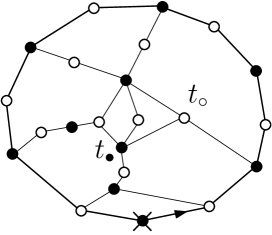
Figure 1. An example of black-rooted bicolored planar map with root face of degree $12$. Each black vertex receives a weight $t_{\bullet}$ and each white vertex a weight $t_{\circ}$, except for the root vertex (origin of the root edge marked by an arrow) which does not receive the weight $t_{\bullet}$, as indicated here conventionally by putting a cross on that vertex.

More precisely, let us define $F_{n}^{\bullet}\equiv F_{n}^{\bullet}(\{g_{k}\}_{k\geq 1},t_{\bullet},t_{\circ})$ as the generating function for black-rooted bicolored planar maps with a root face of degree $2n$. By convention, we decide to assign a weight $1$ to the root face (instead of $g_{n}$) as well as a weight $1$ to the root vertex (instead of $t_{\bullet}$), see Figure 1 for an illustration. We shall also consider the case of maps which are both black-rooted and pointed in such a way that the root vertex is at distance $d_{\bullet}\leq d$ from the pointed vertex and no boundary vertex is at distance strictly less than $d_{\bullet}$ from the pointed vertex (in other words, among all boundary vertices the root vertex is one of the closest ones to the pointed vertex). We shall denote by $F_{n}^{\bullet}(d)$ the corresponding generating function, with now the convention that the pointed vertex receives a weight $1$ (instead of $t_{\bullet}$ or $t_{\circ}$ depending on its color) while the root vertex receives its normal weight $t_{\bullet}$ (unless it is itself the pointed vertex, i.e., when $d_{\bullet}=0$). Note that, in particular

$$F_{n}^{\bullet}=F_{n}^{\bullet}(0)\ .$$

We may finally define similarly generating functions $F_{n}^{\circ}$ and $F_{n}^{\circ}(d)$, now for bicolored planar maps which are white-rooted instead of black-rooted. Clearly, by a symmetry which consists in simply flipping the map and reversing the orientation of the root-edge, keeping all colors unchanged, we have:

(1) $$t_{\bullet}F_{n}^{\bullet}(\{g_{k}\}_{k\geq 1},t_{\bullet},t_{\circ})=t_{\circ}F_{n}^{\circ}(\{g_{k}\}_{k\geq 1},t_{\bullet},t_{\circ})\ .$$

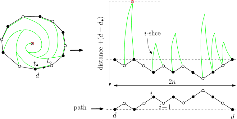
Figure 2. Schematic picture of the slice decomposition of a map contributing to $F_{n}^{\bullet}(d)$. The pointed vertex is represented in red filled with light blue and receives no vertex weight (as indicated by the cross). When each boundary vertex is labelled by its distance to the pointed vertex plus $d-d_{\bullet}$ ($d_{\bullet}$ being the distance from the root vertex to the pointed vertex), the sequence of labels forms a path from height $d$ to height $d$ staying above height $d$ (represented here at the bottom of the figure). Cutting along leftmost geodesic paths from the boundary vertices to the pointed vertex results in a decomposition into slices (upper right part of the figure) with an $i$-slice corresponding to each descending step of the path from height $i$ to height $i-1$ (note that, since distances are measured from the top vertex, the boundary after cutting does not give the desired path but its horizontally reversed image).

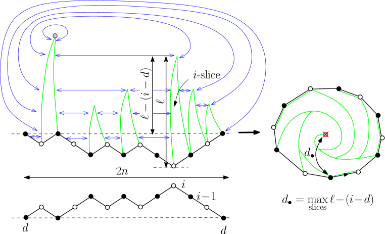
Figure 3. Schematic picture of the reverse construction of the slice decomposition of Figure 2. The map is recovered by gluing the left and right boundaries of the successive slices as indicated by blue arrows. The actual distance $d_{\bullet}$ from the root vertex to the pointed vertex is the maximum over all slices of $\ell-(i-d)$.

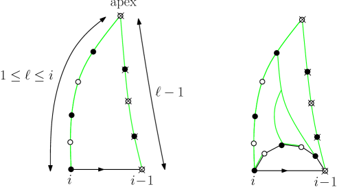
Figure 4. Left: schematic picture of a black $i$-slice. Its left boundary is a geodesic path from the vertex labelled $i$ to the apex, of length $\ell$ for some $1\leq\ell\leq i$. The right boundary is the unique geodesic path from the vertex labelled $i-1$ to the apex and has length $\ell-1$. All vertices receive vertex weights, except those of the right boundary (which includes the apex by convention). Right: schematic picture of the slice decomposition of this $i$-slice (see text).

As discussed in [8], an expression for $F_{n}^{\bullet}(d)$ can be obtained via a so-called slice decomposition as follows : let us view the maps enumerated by $F_{n}^{\bullet}(d)$ as drawn in the plane with the root face as external face and let us label each vertex on the boundary by its distance to the pointed vertex plus $(d-d_{\bullet})$ ($d_{\bullet}$ being the distance of the root vertex to the pointed vertex. In particular the root vertex receives the label $d$). The sequence of these labels when going counterclockwise around the map from the root vertex may be viewed as heights of a path of length $2n$ made of $+1$ or $-1$ steps (each associated to an edge side incident to the root face), starting and ending at height $d$, and remaining above height $d$. The path is naturally colored alternatively in black and white (according to the color of the underlying boundary vertex). We may then draw from each boundary vertex its leftmost geodesic (i.e., shortest) path to the pointed vertex, see Figure 2. The set of these geodesic paths decomposes the map into a number of slices, where a slice is associated to each $-1$ step of the associated path. More precisely, each step $i\to i-1$ gives rise to an $i$-slice, which is a rooted map with the following properties: its boundary is made of three parts, see Figure 4: (i) its base consisting of a single root edge oriented from a vertex labelled $i$ to a vertex labelled $i-1$, (ii) a left boundary of length $\ell$ with $1\leq\ell\leq i$ connecting the vertex labelled $i$ to another vertex, the apex and which is a geodesic path within the slice, and (iii) a right boundary of length $\ell-1$ connecting the vertex labelled $i-1$ to the apex, and which is the unique geodesic path within the slice between these two vertices. By convention, we decide that the apex belongs to the right boundary but not to the left one. The left and right boundaries are then required to have no common vertex (i.e., they do not meet before reaching the apex). The fact that $\ell\leq i$ is simply due to the fact that $\ell$ is smaller than the distance $i-(d-d_{\bullet})$ from the base vertex of the slice labelled $i$ to the pointed vertex in the map. Note that the actual distance $d_{\bullet}$ from the black-root vertex to the pointed vertex is the maximum of $\ell-(i-d)$ over all slices. Note also that, when $\ell=1$, the left boundary may stick to the base, in which case the $i$-slice is reduced to a single edge $i\to i-1$. This degenerate situation occurs whenever the leftmost geodesic path from the boundary vertex labelled $i$ in the original map passes through the next boundary edge counterclockwise around the map (this edge leading to the next boundary vertex counterclockwise around the map, labelled $i-1$). We shall distinguish black $i$-slices, whose root vertex is black from white $i$-slices, whose root vertex is white. The fact that no slice is associated to any $+1$ step in the associated path is because in this case, the leftmost geodesic path from the endpoint (labelled say $i+1$) of the associated $i\to i+1$ boundary edge passes via the origin of the same edge (labelled $i$), hence sticks to the boundary without creating a slice, see Figure 2. The reverse of the slice decomposition is a simple slice concatenation, as shown in Figure 3.

2.2. Continued fractions

In view of the above slice decomposition, it is natural to introduce the generating function $Z_{d,d}^{\bullet\bullet+}(2n)\equiv Z_{d,d}^{\bullet\bullet+}(2n,\{B_{i}\}_{i\geq 1},\{W_{i}\}_{i\geq 1})$ of paths made of $+1$ or $-1$ steps, colored alternatively in black and white, starting and ending at black height $d$ and remaining above height $d$ (with $d\geq 0$), and where each descending step from a black height $i$ to a white height $i-1$ receives a weight $B_{i}$ and each descending step from a white height $i$ to a black height $i-1$ receives a weight $W_{i}$ (and with no weights assigned to ascending steps). More generally, we may define $Z_{d,d^{\prime}}^{\bullet\bullet+}(2n)$ ($d,d^{\prime}\geq 0$) as enumerating paths with the same weights, now going from a black height $d$ to a black height $d^{\prime}$ (with $d^{\prime}=d\mod 2$) and remaining above $\min(d,d^{\prime})$. By obvious generalizations, we shall also consider the quantities $Z_{d,d^{\prime}}^{\circ\circ+}(2n)$ (with $d^{\prime}=d\mod 2$) as well as $Z_{d,d^{\prime}}^{\bullet\circ+}(2n+1)$ and $Z_{d,d^{\prime}}^{\circ\bullet+}(2n+1)$ (with $d^{\prime}=d+1\mod 2$) according to the color of the extremities of the path.

Following [8], the slice decomposition directly gives rise to the following expressions

(2) $$F_{n}^{\bullet}(d)=Z_{d,d}^{\bullet\bullet+}(2n,\{B_{i}\}_{i\geq 1},\{W_{i}\}_{i\geq 1})\qquad\qquad F_{n}^{\circ}(d)=Z_{d,d}^{\circ\circ+}(2n,\{B_{i}\}_{i\geq 1},\{W_{i}\}_{i\geq 1})$$

where $B_{i}\equiv B_{i}(\{g_{k}\}_{k\geq 1},t_{\bullet},t_{\circ})$ (resp. $W_{i}=W_{i}(\{g_{k}\}_{k\geq 1},t_{\bullet},t_{\circ})$) is the generating function for black (resp. white) $i$-slices, see Figure 2. Each face of degree $2k$ in the slice but the root face receives a weight $g_{k}$. As for vertex weights in the slice, they are designed so as to reproduce after concatenation the proper weights for the vertices in the map. To this end, each vertex of the slice receives the weight $t_{\bullet}$ or $t_{\circ}$ according to its color, except for the vertices of the right boundary (including the apex and the base vertex labelled $i-1$) which receive the weight $1$ instead. Indeed, after concatenation of all slices, all the vertices of the map lying on slice boundaries belong to exactly one left boundary hence already receive their weight from this boundary, see Figure 2. This holds except for the pointed vertex, which belongs only to right boundaries hence receives a weight $1$, which is consistent with our convention. Note also, after concatenation of slices, the distance $d_{\bullet}$ from the black-root vertex to the pointed vertex is the maximum of $\ell-(i-d)$ over all slices, hence when $\ell$ varies between $1$ and $i$ for all $i$-slices and with $i$ larger than $d+1$ by construction, $d_{\bullet}$ can be any number between $0$ and $d$.

Taking $d=0$, we deduce in particular

(3) $$F_{n}^{\bullet}=Z_{0,0}^{\bullet\bullet+}(2n,\{B_{i}\}_{i\geq 1},\{W_{i}\}_{i\geq 1})\qquad\qquad F_{n}^{\circ}=Z_{0,0}^{\circ\circ+}(2n,\{B_{i}\}_{i\geq 1},\{W_{i}\}_{i\geq 1})\ .$$

Recall that, by definition, in both path generating functions, each descending step from a black height $i$ to a white height $i-1$ receives the weight $B_{i}$ and each descending step from a white height $i$ to a black height $i-1$ receives the weight $W_{i}$ (and ascending steps receive no weight). With the expressions (3), it is now a standard result that we have the equalities

(4) $$\begin{split}&\sum_{n\geq 0}F_{n}^{\bullet}z^{n}=\frac{1}{\displaystyle{1-z\frac{W_{1}}{\displaystyle{1-z\frac{B_{2}}{\displaystyle{1-z\frac{W_{3}}{\displaystyle{1-z\frac{B_{4}}{\displaystyle{1-\cdots}}}}}}}}}}\\ &\sum_{n\geq 0}F_{n}^{\circ}z^{n}=\frac{1}{\displaystyle{1-z\frac{B_{1}}{\displaystyle{1-z\frac{W_{2}}{\displaystyle{1-z\frac{B_{3}}{\displaystyle{1-z\frac{W_{4}}{\displaystyle{1-\cdots}}}}}}}}}}\\ \end{split}$$

with the convention $F_{0}^{\bullet}=F_{0}^{\circ}=1$, so that $B_{i}$ and $W_{i}$ for $i\geq 1$ can be viewed as the coefficients in the continued fractions of the “resolvents” $\sum_{n\geq 0}F_{n}^{\bullet}z^{n}$ and $\sum_{n\geq 0}F_{n}^{\circ}z^{n}$. Note in particular that, expanding at first order in $z$, eq. (1) yields

(5) $$t_{\bullet}W_{1}=t_{\circ}B_{1}\ .$$

Now it is also a standard result of the theory of continued fractions that, from the first line in (4), we may write for $i\geq 1$

(6) $$B_{2i}=\frac{h_{i}^{(0)}}{h_{i-1}^{(0)}}\Big{/}\frac{h_{i-1}^{(1)}}{h_{i-2}^{(1)}}\qquad\qquad\qquad W_{2i-1}=\frac{h_{i-1}^{(1)}}{h_{i-2}^{(1)}}\Big{/}\frac{h_{i-1}^{(0)}}{h_{i-2}^{(0)}}$$

where $h_{i}^{(0)}$ and $h_{i}^{(1)}$ are Hankel determinants defined from the $F_{n}^{\bullet}$ as

$$h_{i}^{(0)}=\det(F^{\bullet}_{n+m})_{0\leq n,m\leq i}\qquad\qquad h_{i}^{(1)}=\det(F^{\bullet}_{n+m+1})_{0\leq n,m\leq i}$$

with the convention $h_{-1}^{(0)}=h_{-1}^{(1)}=1$. Similarly, the second line in (4) gives, for $i\geq 1$

$$B_{2i-1}=\frac{\tilde{h}_{i-1}^{(1)}}{\tilde{h}_{i-2}^{(1)}}\Big{/}\frac{\tilde{h}_{i-1}^{(0)}}{\tilde{h}_{i-2}^{(0)}}\qquad\qquad\qquad W_{2i}=\frac{\tilde{h}_{i}^{(0)}}{\tilde{h}_{i-1}^{(0)}}\Big{/}\frac{\tilde{h}_{i-1}^{(1)}}{\tilde{h}_{i-2}^{(1)}}$$

where

$$\tilde{h}_{i}^{(0)}=\det(F^{\circ}_{n+m})_{0\leq n,m\leq i}\qquad\qquad\tilde{h}_{i}^{(1)}=\det(F^{\circ}_{n+m+1})_{0\leq n,m\leq i}$$

and again the convention $\tilde{h}_{-1}^{(0)}=\tilde{h}_{-1}^{(1)}=1$. Section 4 below will be devoted to the calculation of the Hankel determinants $h_{i}^{(0)}$, $h_{i}^{(1)}$, $\tilde{h}_{i}^{(0)}$ and $\tilde{h}_{i}^{(1)}$, yielding explicit expressions for the slice generating functions $B_{i}$ and $W_{i}$.

2.3. Link with the two-point function

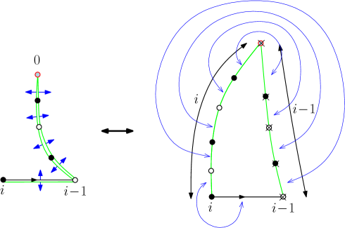
Figure 5. Schematic picture of the bijection between maps contributing to the two-point function $G_{i}^{\bullet}$ and black $i$-slices with a left boundary of length $i$ (i.e., the maximal allowed value).

The reason of our interest in the slice generating functions $B_{i}$ and $W_{i}$ is their intimate link with the distance dependent two-point function. Indeed, let us consider a pointed black-rooted bicolored planar map with a root edge whose black (resp. white) extremity is at graph distance $i$ (resp. $i-1$) from the pointed vertex. By cutting the map along its leftmost geodesic path from the root vertex to the pointed vertex (the first step of the geodesic path being the root edge itself), the resulting object is precisely a black $i$-slice whose left boundary has the maximal allowed length $\ell=i$, see Figure 5. This slice must moreover contain at least one face. For $i>1$, this is automatic but for $i=1$, we must eliminate the slice reduced to a single base edge. This construction is clearly reversible so that the two-point function of bicolored planar maps, defined as the generating function $G_{i}^{\bullet}$ of black-rooted bicolored planar maps with a root edge whose black (resp. white) extremity is at graph distance $i$ (resp. $i-1$) from the pointed vertex, is nothing but the generating function of black $i$-slices with a left boundary of length $i$ (and not reduced to the base edge if $i=1$). For $i>1$, there is an obvious bijection between black $i$-slices with a left boundary of length $1\leq\ell<i$ and black $i-1$-slices of arbitrary left boundary of length $\ell$ ($1\leq\ell\leq i-1$) by simply relabeling the root edge $i-1\to i-2$. We immediately deduce the relations

(7) $$G_{1}^{\bullet}=t_{\circ}(B_{1}-t_{\bullet})\qquad\hbox{and}\quad G_{2i}^{\bullet}=t_{\bullet}(B_{2i}-B_{2i-1})\ ,\quad G_{2i+1}^{\bullet}=t_{\circ}(B_{2i+1}-B_{2i})\quad i>1\ ,$$

where we have re-introduced the weight of the pointed vertex. We may define alternatively the generating function $G_{i}^{\circ}$ of white-rooted bicolored planar maps with a root edge whose white (resp. black) extremity is at graph distance $i$ (resp. $i-1$) from the pointed vertex. Obviously, we have the relations

(8) $$G_{1}^{\circ}=t_{\bullet}(W_{1}-t_{\circ})\qquad\hbox{and}\quad G_{2i}^{\circ}=t_{\circ}(W_{2i}-W_{2i-1})\ ,\quad G_{2i+1}^{\circ}=t_{\bullet}(W_{2i+1}-W_{2i})\quad i>1\ .$$

2.4. Recursive equations for $i$-slice generating functions

As slice generating functions, $B_{i}$ and $W_{i}$ satisfy non-linear recursion relations which can be obtained as follows: assuming $\ell>1$, the face on the left of the root edge of an $i$-slice is necessarily different from the root face and has, say degree $2k$. The set of distances to the apex of the successive vertices, when going around this face of degree $2k$ from the root vertex to the other extremity of the root edge forms a path made of $+1$ and $-1$ steps, of length $2k-1$ from height $i$ to height $i-1$. Drawing from each of these vertices its leftmost geodesic path to the apex results into a slice decomposition of the $i$-slice, see Figure 4, from which we immediately deduce (see [8] for more explanations)

(9) $$\begin{split}&B_{i}=t_{\bullet}+\sum_{k\geq 1}g_{k}Z_{i,i-1}^{\bullet\circ}(2k-1,\{B_{j}\}_{j\geq 1},\{W_{j}\}_{j\geq 1})\\ &W_{i}=t_{\circ}+\sum_{k\geq 1}g_{k}Z_{i,i-1}^{\circ\bullet}(2k-1,\{B_{j}\}_{j\geq 1},\{W_{j}\}_{j\geq 1})\ .\\ \end{split}$$

Here, $Z_{d,d^{\prime}}^{\bullet\circ}(2k-1)$ ($d,d^{\prime}\geq 0,\ d^{\prime}=d+1\mod 2$) denotes the generating function of paths of length $2k-1$ made of $+1$ or $-1$ steps, colored alternatively in black and white, starting at black height $d$ and ending at white height $d^{\prime}$ and remaining above height $0$, where each descending step from a black height $i$ to a white height $i-1$ receives a weight $B_{i}$ and each descending step from a white height $i$ to a black height $i-1$ receives a weight $W_{i}$ (and with no weights assigned to ascending steps). The quantity $Z_{d,d^{\prime}}^{\circ\bullet}(2k-1)$ is defined similarly in an obvious way. The first term $t_{\bullet}$ (resp. $t_{\circ}$) in (LABEL:eq:recurBiWi) arises as the contribution, when $\ell=1$, of the black (resp. white) $i$-slice reduced to a single $i\to i-1$ edge (which receives the weight of the root vertex only since the other vertex belongs to the right boundary).

As an example, let us consider the case of quadrangulations, i.e., maps whose all faces have degree $4$, by taking $g_{k}=\delta_{k,2}$ . The two-point functions $G_{i}^{\bullet}$ and $G_{i}^{\circ}$ for these maps are obtained via (7) and (8) where $B_{i}$ and $W_{i}$ are solutions of the system

(10) $$\begin{split}&B_{i}=t_{\bullet}+Z_{i,i-1}^{\bullet\circ}(3,\{B_{j}\}_{j\geq 1},\{W_{j}\}_{j\geq 1})=t_{\bullet}+B_{i}(W_{i-1}+B_{i}+W_{i+1})\\ &W_{i}=t_{\circ}+Z_{i,i-1}^{\circ\bullet}(3,\{B_{j}\}_{j\geq 1},\{W_{j}\}_{j\geq 1})=t_{\circ}+W_{i}(B_{i-1}+W_{i}+B_{i+1})\\ \end{split}$$

valid for all $i\geq 1$ with the convention $B_{0}=W_{0}=0$. As shown in Appendix A, the solution of these equations may be guessed (with the help of a computer), using the same technique as in [3], based on a perturbative method.

In the case of hexangulations, i.e., maps whose all faces have degree $6$, obtained by taking $g_{k}=\delta_{k,3}$, we get instead

$$\begin{split}&B_{i}=t_{\bullet}+B_{i}(B_{i-2}W_{i-1}\!+\!2B_{i}(W_{i-1}\!+\!W_{i+1})\!+\!B_{i}^{2}\!+\!W_{i-1}^{2}\!+\!W_{i+1}^{2}\!+\!W_{i-1}W_{i+1}\!+\!W_{i+1}B_{i+2})\\ &W_{i}=t_{\circ}+W_{i}(W_{i-2}B_{i-1}\!+\!2W_{i}(B_{i-1}\!+\!B_{i+1})\!+\!W_{i}^{2}+B_{i-1}^{2}\!+\!B_{i+1}^{2}\!+\!B_{i-1}B_{i+1}\!+B_{i+1}W_{i+2})\\ \end{split}$$

valid for all $i\geq 1$ with the convention $B_{0}=W_{0}=B_{-1}=W_{-1}=0$. Note that, in all generality, the equations (LABEL:eq:recurBiWi) form two independent systems of equations, one involving only $B_{i}$’s with even indices $i$ and $W_{j}$’s with odd indices $j$, and one involving only $B_{i}$’s with odd $i$ and $W_{j}$’s with even $j$.

Clearly, in the definition of $i$-slices, the quantity $i$ only acts as an upper bound on the length of the left boundary. We can release this upper bound by simply letting $i\to\infty$ in which case $B_{i}$ and $W_{i}$ tend to well-defined limits $B$ and $W$ solutions of

(11) $$\begin{split}&B=t_{\bullet}+\sum_{k\geq 1}g_{k}\mathbb{Z}_{0,-1}^{\bullet\circ}(2k-1,B,W)\\ &W=t_{\circ}+\sum_{k\geq 1}g_{k}\mathbb{Z}_{0,-1}^{\circ\bullet}(2k-1,B,W)\ .\\ \end{split}$$

where $\mathbb{Z}_{m,n}^{\bullet\circ}(2k-1)\equiv\mathbb{Z}_{m,n}^{\bullet\circ}(2k-1,B,W)$ is the analog of $Z_{m,n}^{\bullet\circ}(2k-1)$ except that heights are allowed to be negative and all descending steps from a black height to a white height receive the same weight $B$ irrespectively of their height, and all descending steps from a white height to a black height receive the same weight $W$. Clearly $\mathbb{Z}_{m,n}^{\bullet\circ}(2k-1)=\mathbb{Z}_{0,n-m}^{\bullet\circ}(2k-1)$ for all $m,n$. We have a similar definition of $\mathbb{Z}_{m,n}^{\circ\bullet}(2k-1)$ and in the following, we shall also consider all variants $\mathbb{Z}_{m,n}^{\bullet\bullet}(2k)$, $\mathbb{Z}_{m,n}^{\bullet\bullet+}(2k)$, … with obvious definitions.

As an example, eqs. (LABEL:eq:recurBW) give for quadrangulations

(12) $$\begin{split}&B=t_{\bullet}+B(B+2W)\\ &W=t_{\circ}+W(W+2B)\\ \end{split}$$

and for hexangulations

(13) $$\begin{split}&B=t_{\bullet}+B(B^{2}+3W^{2}+6BW)\\ &W=t_{\circ}+W(W^{2}+3B^{2}+6BW)\ .\\ \end{split}$$

3. Expressions for $F_{n}^{\bullet}$ and $F_{n}^{\circ}$

3.1. Conserved quantities

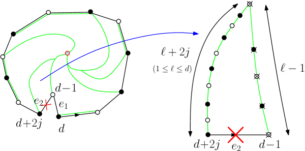
Figure 6. Schematic picture of the map obtained from a map contributing to $F_{n}^{\bullet}(d)$ and having a distance $d_{\bullet}\geq 1$ between the root vertex and the pointed vertex, by cutting along the leftmost edge from the root vertex to a neighboring vertex at distance $d_{\bullet}-1$ from the pointed vertex. After cutting, this edge is split into two edges $e_{1}$ and $e_{2}$, linking vertices with successive labels $d+2j$ (for some $j\geq 1$) , $d-1$ and $d$ counterclockwise, where we use as labels for the boundary vertices $d-d_{\bullet}$ plus their distance to the pointed vertex using paths avoiding $e_{2}$ (as indicated by the red cross). The slice decomposition of this map gives rise to a new type of slice, with base $e_{2}$, whose left boundary now has length $\ell+2j$ and right boundary has length $\ell-1$ for some $\ell$ between $1$ and $d$.

As was done in [8], the quantity $F_{n}^{\bullet}=F_{n}^{\bullet}(0)$ may be obtained by subtracting from $F_{n}^{\bullet}(d)$ the generating function of those configurations having a distance $d_{\bullet}$ strictly positive, i.e., lying between $1$ and $d$ (recall that $d_{\bullet}$ is the distance from the root vertex to the pointed vertex). When $d_{\bullet}\geq 1$, the root vertex has some neighbors at distance $d_{\bullet}-1$ from the pointed vertex which necessarily lie strictly inside the map (i.e., not on the boundary) as otherwise, the root vertex would not be one of the closest vertices to the pointed vertex. Picking the leftmost edge $e$ leading from the root vertex to such a neighbor, we may duplicate this edge by cutting along it and create a map with a boundary of length $2n+2$ whose two new boundary edges are the two copies $e_{1}$ and $e_{2}$ of the edge $e$, with $e_{1}$ say the closest to the root vertex, see Figure 6, so that, counterclockwise around the map, $e_{2}$ links the duplicate of the root vertex to its chosen neighbor at distance $d_{\bullet}-1$, and $e_{1}$ links this neighbor to the original root vertex. We may now apply to this new map the same slice decomposition as before, using now a new graph distance by preventing paths to go through the edge $e_{2}$ and labeling again the boundary vertices by this distance plus $(d-d_{\bullet})$. Because of the new constraint of using only paths avoiding $e_{2}$, the duplicate of the root vertex now receives a label $d+2j$ for some $j\geq 1$ (the fact that the distance to the pointed vertex is strictly larger than $d_{\bullet}$ is due to our choice of leftmost edge, see [8] for a detailed argument). As for all the other boundary vertices, their distance necessarily increases (weakly) in the edge cutting procedure so their label also increases, hence remains above $d$. Moreover, all the obtained slices are $i$-slices as we defined them before except for the last slice whose base is $e_{2}$ which has a left boundary of length $\ell+2j$ for some $\ell$ between $1$ and $d$, and a right boundary of length $\ell-1$ (distances in the slice are also measured with paths avoiding $e_{2}$), see Figure 6. By an argument similar to that used to derive (LABEL:eq:recurBiWi), the generating function for this last slice is

$$\sum_{k\geq 1}g_{k}Z_{d+2j,d-1}^{\bullet\circ}(2k-1,\{B_{j}\}_{j\geq 1},\{W_{j}\}_{j\geq 1})$$

so that the quantity to be subtracted from $F_{n}^{\bullet}(d)$ to get $F_{n}^{\bullet}$ is

$$\frac{1}{t_{\bullet}}\sum_{j\geq 1}Z_{d,d+2j}^{\bullet\bullet+}(2n)\sum_{k\geq 1}g_{k}Z_{d+2j,d-1}^{\bullet\circ}(2k-1)$$

where the role of the factor $1/t_{\bullet}$ is to avoid counting the weight of the original root vertex twice. Using the expression (2) for $F_{n}^{\bullet}(d)$ (and repeating the argument for $F_{n}^{\circ}$), we arrive at

(14) $$\begin{split}&F_{n}^{\bullet}=Z_{d,d}^{\bullet\bullet+}(2n)-\frac{1}{t_{\bullet}}\sum_{j\geq 1}Z_{d,d+2j}^{\bullet\bullet+}(2n)\sum_{k\geq 1}g_{k}Z_{d+2j,d-1}^{\bullet\circ}(2k-1)\\ &F_{n}^{\circ}=Z_{d,d}^{\circ\circ+}(2n)-\frac{1}{t_{\circ}}\sum_{j\geq 1}Z_{d,d+2j}^{\circ\circ+}(2n)\sum_{k\geq 1}g_{k}Z_{d+2j,d-1}^{\circ\bullet}(2k-1)\ .\\ \end{split}$$

The quantities on the right hand side are called conserved quantities to emphasize the fact that their actual values are independent of $d$ (since the left hand size does not depend on $d$).

In the case of quadrangulations for instance taking $n=1$, we get the following conserved quantities

(15) $$\begin{split}&F_{1}^{\bullet}=W_{d+1}-\frac{1}{t_{\bullet}}B_{d}W_{d+1}B_{d+2}=W_{1}=W-\frac{1}{t_{\bullet}}B^{2}W\\ &F_{1}^{\circ}=B_{d+1}-\frac{1}{t_{\circ}}W_{d}B_{d+1}W_{d+2}=B_{1}=B-\frac{1}{t_{\circ}}W^{2}B\\ \end{split}$$

for all $d\geq 0$ (the last two members of the equalities correspond to $d=0$ and $d\to\infty$ respectively).

Note that in this case, a direct proof of this equation may be obtained by writing the relation giving $B_{i}$ in (10) for $i=d+1$, multiplying it by $W_{d}$, then writing the relation giving $W_{i}$ for $i=d$ and multiplying it by $B_{d+1}$ and finally subtracting the two. This leads to $t_{\circ}c_{d}=t_{\bullet}\tilde{c}_{d-1}$ where $c_{d}=B_{d+1}-\frac{1}{t_{\circ}}W_{d}B_{d+1}W_{d+2}$ and $\tilde{c}_{d}=W_{d+1}-\frac{1}{t_{\bullet}}B_{d}W_{d+1}B_{d+2}$. By symmetry, we also have $t_{\bullet}\tilde{c}_{d}=t_{\circ}c_{d-1}$ so that $c_{2i}=\frac{t_{\bullet}}{t_{\circ}}\tilde{c}_{2i-1}=c_{0}=B_{1}$ and $\tilde{c}_{2i}=\frac{t_{\circ}}{t_{\bullet}}c_{2i-1}=\tilde{c}_{0}=W_{1}$ for all $i\geq 1$. This is equivalent to $c_{d}=B_{1}$ and $\tilde{c}_{d}=W_{1}$ for all $d$ thanks to the identity (5). As explained in Appendix A, the use of the above two conserved quantities in the case of quadrangulations allows us to directly derive an explicit expression for $B_{i}$ and $W_{i}$ without recourse to the general formalism that we shall develop below.

3.2. Expression for $F_{n}^{\bullet}$ and $F_{n}^{\circ}$

Expressions (14) for the conserved quantities are particularly interesting as they give expressions for $F_{n}^{\bullet}$ and $F_{n}^{\circ}$ in terms of $B$ and $W$ only, by simply letting $d\to\infty$. Indeed, we immediately get

$$\begin{split}&F_{n}^{\bullet}=\mathbb{Z}_{0,0}^{\bullet\bullet+}(2n)-\frac{1}{t_{\bullet}}\sum_{j\geq 1}\mathbb{Z}_{0,2j}^{\bullet\bullet+}(2n)\sum_{k\geq 1}g_{k}\mathbb{Z}_{2j,-1}^{\bullet\circ}(2k-1)\\ &F_{n}^{\circ}=\mathbb{Z}_{0,0}^{\circ\circ+}(2n)-\frac{1}{t_{\circ}}\sum_{j\geq 1}\mathbb{Z}_{0,2j}^{\circ\circ+}(2n)\sum_{k\geq 1}g_{k}\mathbb{Z}_{2j,-1}^{\circ\bullet}(2k-1)\ .\\ \end{split}$$

Using (LABEL:eq:recurBW), these equations read equivalently

$$\begin{split}&F_{n}^{\bullet}=\frac{1}{t_{\bullet}}\left(B\mathbb{Z}_{0,0}^{\bullet\bullet+}(2n)-\sum_{k\geq 1}g_{k}\sum_{j\geq 0}\mathbb{Z}_{0,2j}^{\bullet\bullet+}(2n)\mathbb{Z}_{2j,-1}^{\bullet\circ}(2k-1)\right)\\ &F_{n}^{\circ}=\frac{1}{t_{\circ}}\left(W\mathbb{Z}_{0,0}^{\circ\circ+}(2n)-\sum_{k\geq 1}g_{k}\sum_{j\geq 0}\mathbb{Z}_{0,2j}^{\circ\circ+}(2n)\mathbb{Z}_{2j,-1}^{\circ\bullet}(2k-1)\right)\\ \end{split}$$

where the sum over $j$ now starts at $j=0$. Now $\sum_{j\geq 0}\mathbb{Z}_{0,2j}^{\bullet\bullet+}(2n)\mathbb{Z}_{2j,-1}^{\bullet\circ}(2k-1)$ enumerates paths form $0$ to $-1$, of total length $2n+2k-1$, and whose $2n$ first steps stay above $0$. Their first $0\to-1$ step therefore occurs after some length $2n+2q$ for some $q\geq 0$. This step receives the weight $B$ and is followed by a path from a white height $-1$ to a white height $-1$ of length $2k-2q-2$ (which thus implies $q\leq k-1$). We may therefore write

$$\begin{split}&\sum_{j\geq 0}\mathbb{Z}_{0,2j}^{\bullet\bullet+}(2n)\mathbb{Z}_{2j,-1}^{\bullet\circ}(2k-1)=B\sum_{q=0}^{k-1}\mathbb{Z}_{0,0}^{\bullet\bullet+}(2n+2q)\mathbb{Z}_{-1,-1}^{\circ\circ}(2k-2q-2)\\ &\sum_{j\geq 0}\mathbb{Z}_{0,2j}^{\circ\circ+}(2n)\mathbb{Z}_{2j,-1}^{\circ\bullet}(2k-1)=W\sum_{q=0}^{k-1}\mathbb{Z}_{0,0}^{\circ\circ+}(2n+2q)\mathbb{Z}_{-1,-1}^{\bullet\bullet}(2k-2q-2)\\ \end{split}$$

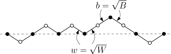
Figure 7. Path weights for the generating functions $\hat{\mathbb{Z}}$. A weight is assigned to both descending and ascending steps: $b=\sqrt{B}$ if the lower height is white and $w=\sqrt{W}$ if the lower height is black.

So far all path weights have been assigned to descending steps only. From now on we shall use slightly different conventions for path weights by assigning, see Figure 7:

• a weight $b=\sqrt{B}$ to each descending step from a black height to a white height and to each ascending step from a white height to a black height ;

• a weight $w=\sqrt{W}$ to each descending step from a white height to a black height and to each ascending step from a black height to a white height.

We shall denote by $\hat{\mathbb{Z}}$ (instead of $\mathbb{Z}$) the corresponding generating functions. Clearly, when the heights of the two extremities of the path are the same, the ascending and descending steps of each sort are well balanced so that, for instance $\mathbb{Z}_{0,0}^{\bullet\bullet+}(2n+2q)=\hat{\mathbb{Z}}_{0,0}^{\bullet\bullet+}(2n+2q)$ and $\mathbb{Z}_{-1,-1}^{\circ\circ}(2k-2q-2)=\hat{\mathbb{Z}}_{-1,-1}^{\circ\circ}(2k-2q-2)$. Moreover, by reversing the paths vertically, we have $\hat{\mathbb{Z}}_{0,-2k}^{\bullet\bullet}(2n)=\hat{\mathbb{Z}}_{-2k,0}^{\bullet\bullet}(2n)$ since the weights are unchanged under reversing. If we now reverse the paths horizontally, we get instead $\hat{\mathbb{Z}}_{-2k,0}^{\bullet\bullet}(2n)=\hat{\mathbb{Z}}_{0,-2k}^{\circ\circ}(2n)$ since under this reversing, the colors have to be exchanged for the weights $b$ and $w$ to remain correct. We may thus introduce the function

(16) $$L_{k}(2n)\equiv\hat{\mathbb{Z}}_{i,i-2k}^{\bullet\bullet}(2n)=\hat{\mathbb{Z}}_{i,i-2k}^{\circ\circ}(2n)$$

(note that the last two terms are indeed independent of $i$) and it satisfies the relation

$$L_{k}(2n)=L_{-k}(2n)\ .$$

With these new notations, we end up with

(17) $$\begin{split}&F_{n}^{\bullet}=\sum_{g\geq 0}\alpha_{q}\hat{\mathbb{Z}}_{0,0}^{\bullet\bullet+}(2n+2q)\qquad\alpha_{q}=\frac{B}{t_{\bullet}}\left(\delta_{q,0}-\sum_{k\geq q+1}g_{k}L_{0}(2k-2q-2)\right)\\ &F_{n}^{\circ}=\sum_{g\geq 0}\tilde{\alpha}_{q}\hat{\mathbb{Z}}_{0,0}^{\circ\circ+}(2n+2q)\qquad\tilde{\alpha}_{q}=\frac{W}{t_{\circ}}\left(\delta_{q,0}-\sum_{k\geq q+1}g_{k}L_{0}(2k-2q-2)\right)\\ \end{split}$$

To illustrate this formula, let us return to the case of quadrangulations (where $g_{2}$ is omitted). In this case, only $\alpha_{0}$ and $\alpha_{1}$ are non-zero, and have values

$$\begin{split}&\alpha_{0}=\frac{B}{t_{\bullet}}(1-L_{0}(2))=\frac{B}{t_{\bullet}}(1-(B+W))=1+\frac{BW}{t_{\bullet}}\\ &\alpha_{1}=\frac{B}{t_{\bullet}}(-L_{0}(0))=-\frac{B}{t_{\bullet}}\\ &\tilde{\alpha}_{0}=\frac{W}{t_{\circ}}(1-L_{0}(2))=\frac{W}{t_{\circ}}(1-(B+W))=1+\frac{BW}{t_{\circ}}\\ &\tilde{\alpha}_{1}=\frac{W}{t_{\circ}}(-L_{0}(0))=-\frac{W}{t_{\circ}}\ .\\ \end{split}$$

Here we have used eqs. (LABEL:eq:recurBWquad) to simplify the first and third lines. This leads to

$$\begin{split}F_{1}^{\bullet}=&\alpha_{0}\hat{\mathbb{Z}}_{0,0}^{\bullet\bullet+}(2)+\alpha_{1}\hat{\mathbb{Z}}_{0,0}^{\bullet\bullet+}(4)\\ &=\alpha_{0}W+\alpha_{1}(W^{2}+BW)=W-\frac{1}{t_{\bullet}}B^{2}W\\ F_{1}^{\circ}=&\tilde{\alpha}_{0}\hat{\mathbb{Z}}_{0,0}^{\circ\circ+}(2)+\tilde{\alpha}_{1}\hat{\mathbb{Z}}_{0,0}^{\circ\circ+}(4)\\ &=\tilde{\alpha}_{0}B+\tilde{\alpha}_{1}(B^{2}+BW)=B-\frac{1}{t_{\circ}}W^{2}B\\ \end{split}$$

in agreement with eqs. (15).

4. Computation of the Hankel determinants

4.1. Computation of $h_{i}^{(1)}$ and $\tilde{h}_{i}^{(1)}$

The computation of $h_{i}^{(1)}$ and $\tilde{h}_{i}^{(1)}$ turns out to be simple as it takes exactly the same form as that performed in [8]. Indeed, we may use the relation

$$\hat{\mathbb{Z}}_{0,0}^{\bullet\bullet+}(2m+2n+2+2q)=\sum_{k=1}^{m+1}\sum_{\ell=1}^{n+1}\hat{\mathbb{Z}}_{0,2k-1}^{\bullet\circ+}(2m+1)A_{2k-1,2\ell-1}^{\circ\circ}(2q)\hat{\mathbb{Z}}_{2\ell-1,0}^{\circ\bullet+}(2n+1)$$

obtained by classifying the paths according to the heights $2k-1$ and $2\ell-1$ after $2m+1$ and $2m+1+2q$ steps. Here $A_{2k-1,2\ell-1}^{\circ\circ}(2q)$ denotes the generating function of paths of length $2q$ from white height $2k-1$ to white height $2\ell-1$ (with the weights $b=\sqrt{B}$ and $w=\sqrt{W}$ assigned to both ascending and descending steps according to the color of their extremities) which remain above height $0$ (note that height $0$ is black in this case).

This results into the matrix identity

$$(F_{n+m+1}^{\bullet})_{0\leq m,n\leq i}=(\hat{\mathbb{Z}}_{0,2k-1}^{\bullet\circ+}(2m+1))_{0\leq m\leq i\atop 1\leq k\leq i+1}\cdot(\sum_{q\geq 0}\alpha_{q}A_{2k-1,2\ell-1}^{\circ\circ}(2q))_{1\leq k,\ell\leq i+1}\cdot(\hat{\mathbb{Z}}_{2\ell-1,0}^{\circ\bullet+}(2n+1))_{1\leq\ell\leq i+1\atop 0\leq n\leq i}$$

Taking the determinant of both sides of this identity and noting that the two extremal matrices in the right hand side are triangular matrices whose determinants are trivially computed, we immediately get to

$$h_{i}^{(1)}=W^{i+1}(BW)^{\frac{i(i+1)}{2}}\det_{1\leq k,\ell\leq i+1}(\sum_{q\geq 0}\alpha_{q}A_{2k-1,2\ell-1}^{\circ\circ}(2q))$$

and similarly

$$\tilde{h}_{i}^{(1)}=B^{i+1}(BW)^{\frac{i(i+1)}{2}}\det_{1\leq k,\ell\leq i+1}(\sum_{q\geq 0}\alpha_{q}A_{2k-1,2\ell-1}^{\bullet\bullet}(2q))$$

where $A_{2k-1,2\ell-1}^{\bullet\bullet}(2q)$ now denotes the generating function of paths of length $2q$ from black height $2k-1$ to black height $2\ell-1$ (with the weights $b=\sqrt{B}$ and $w=\sqrt{W}$ assigned to both ascending and descending steps according to the color of their extremities) which remain above height $0$ (height $0$ being white in this case).

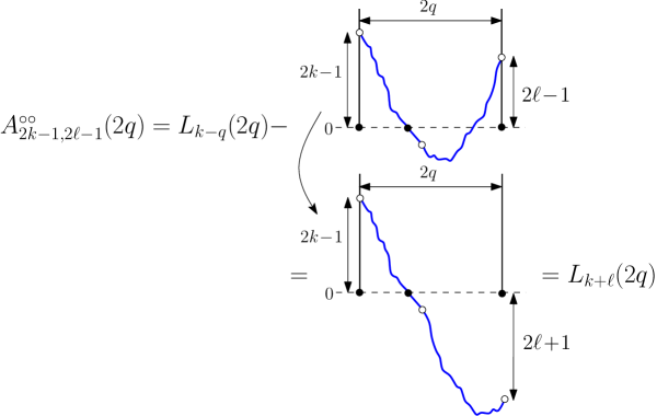
Figure 8. By a standard reflection principle, $A_{2k-1,2\ell-1}^{\circ\circ}(2q)$ is obtained by subtracting from $L_{k-\ell}(2q)$ paths which go below $0$, which are in bijection with paths with height decrease $(k+\ell)$, as enumerated by $L_{k+\ell}(2q)$. Note that the rightmost part of the path has been returned vertically in the argument in order for the weights after reversing to still be correct.

Let us from now on concentrate on $h_{i}^{(1)}$. The quantity $A_{2k-1,2\ell-1}^{\circ\circ}(2q)$ may be obtained via a simple (and standard) reflection principle, namely

$$A_{2k-1,2\ell-1}^{\circ\circ}(2q)=L_{k-\ell}(2q)-L_{k+\ell}(2q)\ .$$

Indeed, paths contributing to $A_{2k-1,2\ell-1}^{\circ\circ}(2q)$ are identical to those which contribute to $\hat{\mathbb{Z}}_{2k-1,2\ell-1}^{\circ\circ}(2q)=L_{k-\ell}(2q)$ except that they have to remain above height $0$. The paths to be subtracted are those paths reaching a negative height. Considering the first step on the negative side (this $0\to-1$ step receives the weight $b=\sqrt{B}$ since height $0$ is black), the rest of the path goes from a white height $-1$ to a white height $2\ell-1$. Returning this path vertically (which does not modify the weight prescription), see Figure 8, and shifting the heights by $2\ell$, we get a properly weighted path from height $2k-1$ to height $-1-2\ell$, as enumerated by $\hat{\mathbb{Z}}_{2k-1,-1-2\ell}^{\circ\circ}(2q)=L_{k+\ell}(2q)$, hence the formula. We deduce

(18) $$h_{i}^{(1)}=W^{i+1}(BW)^{\frac{i(i+1)}{2}}\det_{1\leq k,\ell\leq i+1}(C_{k-\ell}-C_{k+\ell})$$

where

$$C_{k}=\sum_{q\geq 0}\alpha_{q}L_{k}(2q)\ .$$

From now on, we shall assume that the $g_{k}$’s for $k>p+1$ are all $0$ and that $g_{p+1}\neq 0$, for some $p\geq 1$. In other words, we enumerate maps with faces of degree at most $2p+2$. The case of quadrangulations corresponds to $p=1$ (and $g_{1}=0$) and that of hexangulations to $p=2$ (and $g_{1}=g_{2}=0$). Note in this case that $\alpha_{q}=0$ for $q>p$, hence, from its definition, $C_{k}=0$ for $|k|>p$, while

$$C_{p}=C_{-p}=-\frac{B}{t_{\bullet}}g_{p+1}(BW)^{p/2}\ .$$

A simple formula can then be written for the determinant appearing in eq. (18) in terms of the solutions $x_{a}$ of the so-called characteristic equation

(19) $$0=\sum_{k=-p}^{p}C_{k}x^{k}=C_{0}+\sum_{k=1}^{p}C_{k}\left(x^{k}+\frac{1}{x^{k}}\right)$$

since $L_{k}(2q)=L_{-k}(2q)$, hence $C_{k}=C_{-k}$. This equation has $2p$ solutions which we denote by $x_{a}$ and $1/x_{a}$, $a=1,\cdots,p$ ($x_{a}$ being chosen, say with modulus less than $1$). The $p$ quantities $x_{a}$ may be viewed as a parametrization of the $p$ quantities $C_{0},C_{1},\cdots C_{p-1}$ via

(20) $$C_{k}=(-1)^{p+k}C_{p}e_{p+k}\left(x_{1},x_{2},\dots,x_{p},\frac{1}{x_{1}},\frac{1}{x_{2}},\cdots,\frac{1}{x_{p}}\right)$$

where the $e_{i}$’s denote the usual elementary symmetric polynomials. It is now a standard result of representation theory [12] (already used in [8]) that

(21) $$\det\limits_{1\leq k,\ell\leq i+1}(C_{k-\ell}-C_{k+\ell})=(-1)^{p(i+1)}C_{p}^{i+1}\frac{\det\limits_{1\leq a,a^{\prime}\leq p}(x_{a}^{i+1+a^{\prime}}-x_{a}^{-(i+1+a^{\prime})})}{\det\limits_{1\leq a,a^{\prime}\leq p}(x_{a}^{a^{\prime}}-x_{a}^{-a^{\prime}})}\ .$$

This leads eventually to

(22) $$h_{i}^{(1)}=W^{i+1}(BW)^{\frac{i(i+1)}{2}}(-1)^{p(i+1)}C_{p}^{i+1}\frac{\det\limits_{1\leq a,a^{\prime}\leq p}(x_{a}^{i+1+a^{\prime}}-x_{a}^{-(i+1+a^{\prime})})}{\det\limits_{1\leq a,a^{\prime}\leq p}(x_{a}^{a^{\prime}}-x_{a}^{-a^{\prime}})})$$

and, by a similar argument

$$\tilde{h}_{i}^{(1)}=B^{i+1}(BW)^{\frac{i(i+1)}{2}}(-1)^{p(i+1)}\tilde{C}_{p}^{i+1}\frac{\det\limits_{1\leq a,a^{\prime}\leq p}(x_{a}^{i+1+a^{\prime}}-x_{a}^{-(i+1+a^{\prime})})}{\det\limits_{1\leq a,a^{\prime}\leq p}(x_{a}^{a^{\prime}}-x_{a}^{-a^{\prime}})})$$

with $\tilde{C}_{p}=-\frac{W}{t_{\circ}}g_{p+1}(BW)^{p/2}$. Note that, since the $\alpha_{q}$’s and the $\tilde{\alpha}_{q}$’s are proportional, and because of (16), the characteristic equation is the same in the calculation of $\tilde{h}_{i}^{(1)}$ as that for $h_{i}^{(1)}$, hence the $x_{a}$’s are the same.

As just mentioned, eq. (21) is a standard result of representation theory, whose proof can be found in Appendix A of [12]. Still, the proof of [12] is not so enlightening to the neophyte and it is instructive to recover this result via a more heuristic argument. From the characteristic equation, we deduce that the vectors $(x_{a}^{\ell})_{\ell\in\mathbb{Z}}$ and $(x_{a}^{-\ell})_{\ell\in\mathbb{Z}}$ (for any $x_{a}$ solution of the characteristic equation) are both in the kernel of the infinite matrix $(C_{k-\ell})_{k,\ell\in\mathbb{Z}}$, namely

$$\sum_{\ell\in\mathbb{Z}}C_{k-\ell}x_{a}^{\ell}=x_{a}^{k}(\sum_{m\in\mathbb{Z}}C_{m}x_{a}^{-m})=0\qquad\sum_{\ell\in\mathbb{Z}}C_{k-\ell}x_{a}^{-\ell}=x_{a}^{-k}(\sum_{m\in\mathbb{Z}}C_{m}x_{a}^{m})=0$$

for $a=1,\cdots,p$ (recall that $C_{m}=C_{-m}$). To now find a vector $v_{\ell}$ in the kernel of the semi-infinite matrix $(C_{k-\ell}-C_{k+\ell})_{k,\ell\geq 1}$, we note that, for $k\geq 1$

$$\begin{split}\sum_{\ell\geq 1}(C_{k-\ell}-C_{k+\ell})v_{\ell}&=\sum_{\ell\geq 1}C_{k-\ell}v_{\ell}-\sum_{\ell\leq-1}C_{k-\ell}v_{-\ell}\\ &=\sum_{\ell\in\mathbb{Z}}C_{k-\ell}v_{\ell}\\ \end{split}$$

provided $v_{-\ell}=-v_{\ell}$ for all $\ell$ (in particular $v_{0}=0$). For $a=1,\cdots,p$, the vectors with components

(23) $$v_{\ell}^{(a)}=x_{a}^{\ell}-x_{a}^{-\ell}\qquad\ell\geq 1$$

are therefore in the kernel of our semi-infinite matrix. Taking now $k\leq i+1$, the sum over all $\ell\geq 1$ runs in practice only from $1$ to $i+p+1$ so that we get a vector satisfying

$$\sum_{\ell=1}^{i+1}(C_{k-\ell}-C_{k+\ell})v_{\ell}=0$$

by simply imposing $v_{i+2}=v_{i+3}=\cdots=v_{i+p+1}=0$. These extra conditions can be achieved by taking a linear combination of the $p$ vectors $(v_{\ell}^{(a)})_{\ell\geq 1}$ and lead to a non-zero vector if the $p$ conditions are not linearly independent, namely whenever

$$\det_{1\leq a,a^{\prime}\leq p}v_{i+a^{\prime}+1}^{(a)}=0\ .$$

The determinant in the left hand side of (21) therefore vanishes whenever the determinant $\det_{1\leq a,a^{\prime}\leq p}v_{i+a^{\prime}+1}^{(a)}$ vanishes. This latter determinant (which is anti-symmetric in the $x_{a}$’s instead of the desired determinant which is symmetric) has however more zeros than desired: it indeed vanishes whenever $x_{a}=x_{a^{\prime}}$ for some $a\neq a^{\prime}$ (as it implies $v_{\ell}^{(a)}=v_{\ell}^{(a^{\prime})}$) or $x_{a}=1/x_{a^{\prime}}$ for any $a,a^{\prime}$ (as it implies $v_{\ell}^{(a)}=-v_{\ell}^{(a^{\prime})}$), and in particular (for $a=a^{\prime}$) when $x_{a}=\pm 1$ (in which case $v_{\ell}^{(a)}=0$). These cases correspond precisely to the zeros of $\det_{1\leq a,a^{\prime}\leq p}v_{a^{\prime}}^{(a)}=(-1)^{p}\prod_{a=1}^{p}(1-x_{a}^{2})\prod_{1\leq a<a^{\prime}\leq p}(x_{a}-x_{a^{\prime}})(1-x_{a}x_{a^{\prime}})/\prod_{a=1}^{p}x_{a}^{p}$ and we must suppress them by dividing $\det_{1\leq a,a^{\prime}\leq p}v_{i+a^{\prime}+1}^{(a)}$ by $\det_{1\leq a,a^{\prime}\leq p}v_{a^{\prime}}^{(a)}$. This eventually explains (21) by adjusting the proportionality constant so that, say the $(x_{1}x_{2}\cdots x_{p})^{i+1}$ term on both sides be the same. Indeed, in the left hand side, this term comes from the largest possible power of $C_{0}$, namely $C_{0}^{i+1}$, leading to a term $((-1)^{p}C_{p})^{i+1}$, while in the ratio of determinants in the right hand side, it is easily seen to be $1$.

We gave here the argument as we find it more enlightening than the proof in [12]. Still, as presented here, this is just an argument and promoting it into a real proof would need a better control on the various determinants involved (in particular deal with the possibility of multiple roots, …).

To illustrate our result, let us give the expression for $h_{i}^{(1)}$ in the case of quadrangulations and hexangulations. For quadrangulations, we have $p=1$ and $C_{p}=-\frac{B}{t_{\bullet}}(BW)^{1/2}$, so that

(24) $$h_{i}^{(1)}=W^{i+1}(BW)^{\frac{(i+1)^{2}}{2}}\left(\frac{B}{t_{\bullet}}\right)^{i+1}\frac{1}{x^{i+1}}\frac{1}{1-x^{2}}\,u_{2i+4}\ \hbox{where}\ u_{i}\equiv 1-x^{i}\ ,$$

with $B$ and $W$ solutions of (LABEL:eq:recurBWquad), and where $x$ is the solution (with modulus less than one) of the characteristic equation (obtained after some straightforward simplifications)

(25) $$1-2(B+W)-\sqrt{BW}\left(x+\frac{1}{x}\right)=0\ .$$

As for hexangulation ($p=2$ and $C_{p}=-\frac{B}{t_{\bullet}}(BW)$), we get

(26) $$\begin{split}h_{i}^{(1)}&=W^{i+1}(BW)^{\frac{(i+1)(i+2)}{2}}\left(-\frac{B}{t_{\bullet}}\right)^{i+1}\frac{1}{(x_{1}x_{2})^{i+1}}\frac{1}{1-x_{1}^{2}}\frac{1}{1-x_{2}^{2}}\frac{1}{1-x_{1}x_{2}}\,u_{2i+4}\\ &\hbox{where}\ u_{i}\equiv 1-\frac{1-x_{1}x_{2}}{x_{1}-x_{2}}x_{1}^{i+1}-\frac{1-x_{1}x_{2}}{x_{2}-x_{1}}x_{2}^{i+1}-(x_{1}x_{2})^{i+1}\\ \end{split}$$

with $B$ and $W$ solutions of (LABEL:eq:recurBWhex), and where $x_{1}$ and $x_{2}$ are the solutions (with modulus less than one) of

(27) $$1-3(B^{2}+W^{2})-10BW-3\sqrt{BW}(B+W)\left(x+\frac{1}{x}\right)-BW\left(x^{2}+\frac{1}{x^{2}}\right)=0\ .$$

4.2. Computation of $h_{i}^{(0)}$ and $\tilde{h}_{i}^{(0)}$

By an argument similar to the previous subsection, we immediately get

(28) $$\begin{split}&h_{i}^{(0)}=(BW)^{\frac{i(i+1)}{2}}\det_{0\leq k,\ell\leq i}(\sum_{q\geq 0}\alpha_{q}A_{2k,2\ell}^{\bullet\bullet}(2q))\\ &\tilde{h}_{i}^{(0)}=(BW)^{\frac{i(i+1)}{2}}\det_{0\leq k,\ell\leq i}(\sum_{q\geq 0}\alpha_{q}A_{2k,2\ell}^{\circ\circ}(2q))\\ \end{split}$$

where $A_{2k,2\ell}^{\bullet\bullet}(2q)$ denotes the generating function of paths of length $2q$ from black height $2k$ to black height $2\ell$ which remain above height $0$ (note that height $0$ is black in this case) and $A_{2k,2\ell}^{\circ\circ}(2q)$ denotes the generating function of paths of length $2q$ from white height $2k$ to white height $2\ell$ which remain above height $0$ (note that height $0$ is white in this case). The difficulty is now that, because of the (even) parity of the heights of the extremities of the path, we can no longer use a reflection principle as simple as that of the previous section. Nevertheless, we have the following formula, for $k,\ell\geq 0$:

(29) $$A_{2k,2\ell}^{\bullet\bullet}(2q)=L_{k-\ell}(2q)-c\,L_{k+\ell+1}(2q)+(c^{2}-1)\sum_{m\geq 2}L_{k+\ell+m}(2q)(-c)^{m-2}$$

where

$$c\equiv\frac{b}{w}=\sqrt{\frac{B}{W}}$$

and a similar expression for $A_{2k,2\ell}^{\circ\circ}(2q)$ with $b$ and $w$ exchanged, i.e., with $c\to 1/c$. This in turn implies

(30) $$\sum_{q\geq 0}\alpha_{q}A_{2k,2\ell}^{\bullet\bullet}(2q)=C_{k-\ell}-c\,C_{k+\ell+1}+(c^{2}-1)\sum_{m\geq 2}C_{k+\ell+m}(-c)^{m-2}\ .$$

Note that the sum in the right hand side is in practice finite.

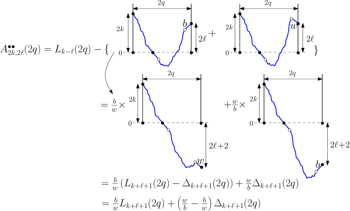
Figure 9. We get $A_{2k,2\ell}^{\bullet\bullet}(2q)$ by subtracting from $L_{k-\ell}(2q)$ paths which go below $0$, which are decomposed in two sets: those ending with an up step (weighted $b$) and those ending with a down step (weighted $w$). By returning vertically the rightmost part of the paths but the last step which we return horizontally, we get paths with height decrease $2(k+\ell+1)$. To get the correct weights, we must apply a multiplicative factor $b/w$ to the first set (enumerated by $L_{k+\ell+1}(2q)-\Delta_{k+\ell+1}(2q)$) and a multiplicative factor $w/b$ to the second set (enumerated by $\Delta_{k+\ell+1}(2q)$), hence the formula.

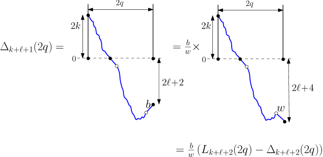
Figure 10. By simply returning the last step horizontally, we see that the generating function $\Delta_{k+\ell+1}(2q)$ for paths of length $2q$, height decrease $2(k+\ell+1)$ and ending with an up step is $(b/w)$ times the generating function $L_{k+\ell+2}(2q)-\Delta_{k+\ell+2}(2q)$ for paths of length $2q$, height decrease $2(k+\ell+2)$ and ending with a down step. By repeating this argument recursively, we find that $\Delta_{k+\ell+1}(2q)=-\sum_{m\geq 2}\left(-\frac{b}{w}\right)^{m-1}L_{k+\ell+m}(2q)$.

Let us now explain the formula (29). We may assume $q>0$ since, for $q=0$, the formula is obvious (only the first term in the right hand side contributes). To get $A_{2k,2\ell}^{\bullet\bullet}(2q)$, we wish as before to subtract from $L_{k-\ell}(2q)$ the generating function of those paths which go below height $0$. To apply again some reflection principle, we look at the first passage below $0$, which is a step from a black height $0$ to a white height $-1$ (hence receives a weight $b$). The rest of the path is formed of an “intermediate” part going from white height $-1$ to the last encountered white height (equal to $2\ell+1$ or $2\ell-1$) and of a final step reaching black height $2\ell$, see Figure 9. If we now return vertically the intermediate part and horizontally the last step, we get a total path of length $2q$ going from height $2k$ to height $-2-2\ell$, hence with height decrease $2(k+\ell+1)$. The weights of all steps after reversing are correct (recall that a vertical reversing conserves the weights) except for that of the last step which is $b$ (before reversing) instead of $w$ (as required after reversing) if the last step after reversing is a descending step from white height $-1-2\ell$ to black height $-2-2\ell$ or is $w$ (before reversing) instead of $b$ (after reversing) if the last step after reversing is an ascending step from white height $-3-2\ell$ to black height $-2-2\ell$, see Figure 10. Both kinds of paths are enumerated by $L_{k+\ell+1}(2q)$ but for the first kind, we must apply a multiplicative correction $b/w$ while for the second kind, we must apply a multiplicative correction $w/b$. The quantity $L_{k-\ell}(2q)-(b/w)L_{k+\ell+1}(2q)$ therefore performs the correct subtraction of paths of the first kind but paths of the second kind must be re-added with a multiplicative factor $(b/w-w/b)$ to obtain a correct result. If we denote by $\Delta_{k+\ell+1}(2q)$ the generating function of those paths, the correct formula is therefore $A_{2k,2\ell}^{\bullet\bullet}(2q)=L_{k-\ell}(2q)-(b/w)\,L_{k+\ell+1}(2q)+(b/w-w/b)\Delta_{k+\ell+1}(2q)$. Now, by returning the last (ascending) step in a path enumerated by $\Delta_{k+\ell+1}(2q)$, we get a path whose last step is now descending from white height $-3-2\ell$ to black height $-4-2\ell$, hence a path with height decrease $2(k+\ell+2)$ and, in our terminology, being of the first kind. This immediately leads to the relation $\Delta_{k+\ell+1}(2q)=\frac{b}{w}(L_{k+\ell+2}(2q)-\Delta_{k+\ell+2}(2q))$ and, by repeating the argument recursively to $\Delta_{k+\ell+1}(2q)=-\sum_{m\geq 2}\left(-\frac{b}{w}\right)^{m-1}L_{k+\ell+m}(2q)$. Setting $c=b/w$ yields eventually the desired formula (29). To conclude, let us mention that we have a formula for $A_{2k,2\ell}^{\circ\circ}(2q)$ similar to (29) with $c$ changed into $1/c$.

With the above formula (30), the computation of the determinants in eqs. (28) is much more involved and we detail it in Appendix B. Still the result is remarkably simple as we get eventually

(31) $$\begin{split}h_{i}^{(0)}&=(BW)^{\frac{i(i+1)}{2}}(-1)^{p(i+1)}C_{p}^{i+1}\prod_{a=1}^{p}(1+c\,x_{a})\frac{\det\limits_{1\leq a,a^{\prime}\leq p}(\gamma_{a}x_{a}^{i+a^{\prime}}-x_{a}^{-(i+1+a^{\prime})})}{\det\limits_{1\leq a,a^{\prime}\leq p}(x_{a}^{a^{\prime}}-x_{a}^{-a^{\prime}})})\\ &\qquad\hbox{where}\ \gamma_{a}=\frac{c+x_{a}}{1+cx_{a}}\\ \end{split}$$

while

(32) $$\tilde{h}_{i}^{(0)}=(BW)^{\frac{i(i+1)}{2}}(-1)^{p(i+1)}\tilde{C}_{p}^{i+1}\prod_{a=1}^{p}(1+x_{a}/c)\frac{\det\limits_{1\leq a,a^{\prime}\leq p}(x_{a}^{i+a^{\prime}}/\gamma_{a}-x_{a}^{-(i+1+a^{\prime})})}{\det\limits_{1\leq a,a^{\prime}\leq p}(x_{a}^{a^{\prime}}-x_{a}^{-a^{\prime}})})$$

(note the change $c\to 1/c$, which in turn implies the change $\gamma_{a}\to 1/\gamma_{a}$). Note also that both $h_{i}^{(0)}$ and $\tilde{h}_{i}^{(0)}$ are actually invariant under $x_{a}\leftrightarrow 1/x_{a}$ for any $a$ since $(1+c\,x_{a})(\gamma_{a}x_{a}^{i+a^{\prime}}-x_{a}^{-(i+1+a^{\prime})})=(x_{a}^{i+a^{\prime}+1}-x_{a}^{-(i+a^{\prime}+1)})+c(x_{a}^{i+a^{\prime}}-x_{a}^{-(i+a^{\prime})})$.

Again, besides the actual proof of Appendix B, we can give a more heuristic argument along the same lines as before. Writing

$$\begin{split}\sum_{\ell\geq 0}\left(\sum_{q\geq 0}A_{2k,2\ell}^{\bullet\bullet}(2q)\right)w_{\ell}&=\sum_{\ell\geq 0}\big{(}C_{k-\ell}-c\,C_{k+\ell+1}+(c^{2}-1)\sum_{m\geq 2}C_{k+\ell+m}(-c)^{m-2}\big{)}w_{\ell}\\ &=\sum_{\ell\geq 0}C_{k-\ell}w_{\ell}-c\sum_{\ell\leq-1}C_{k-\ell}w_{-\ell-1}\\ &\hskip 85.35826pt+(c^{2}-1)\sum_{m\geq 2}(-c)^{m-2}\sum_{\ell\leq-m}C_{k-\ell}w_{-\ell-m}\\ \end{split}$$

we see that, for $\ell\leq-1$, the net coefficient in front of $C_{k-\ell}$ is

$$-c\,w_{-\ell-1}+(c^{2}-1)\sum_{m=2}^{-\ell}(-c)^{m-2}w_{-\ell-m}$$

while we would have liked it to be $w_{\ell}$ so as to reproduce $\sum_{\ell\in\mathbb{Z}}C_{k-\ell}w_{\ell}$ which is known to give $0$ for $w_{\ell}=x_{a}^{\ell}$ or $w_{\ell}=x_{a}^{-\ell}$. To construct a vector in the kernel of $(\sum_{q\geq 0}A_{2k,2\ell}^{\bullet\bullet}(2q))_{k,\ell\geq 0}$, we thus may as before take a linear combination of $x_{a}^{\ell}$ or $x_{a}^{-\ell}$, now satisfying for all $\ell\leq-1$ the condition

$$w_{\ell}=-c\,w_{\ell-1}+(c^{2}-1)\sum_{m=2}^{-\ell}(-c)^{m-2}w_{-\ell-m}$$

(the sum being empty if $\ell=-1$). Writing $(c^{2}-1)\sum_{m=2}^{-\ell}(-c)^{m-2}w_{\ell-m}=(c^{2}-1)w_{-\ell-2}-c(c^{2}-1)\sum_{m=2}^{-\ell-1}(-c)^{m-2}w_{-\ell-1-m}$ and using the above condition for $\ell+1$, we obtain that this condition is equivalent recursively (over $|\ell|=-\ell$) to $w_{\ell}=-c\,w_{\ell-1}+(c^{2}-1)w_{-\ell-2}-c\big{(}w_{\ell+1}+c\,w_{-\ell-2})\big{)}$, namely

$$(w_{\ell}+w_{-\ell-2})+c(w_{\ell+1}+w_{-\ell-1})=0$$

for all $\ell\leq-1$ (i.e., for all $\ell$ since it is symmetric under $\ell\to-\ell-2$). This leads immediately to the linear combination

$$w_{\ell}^{(a)}=\frac{c+x_{a}}{1+c\,x_{a}}x_{a}^{\ell}-x_{a}^{-\ell-1}\qquad\ell\geq 0$$

for $a=1,\cdots,p$, which satisfy

$$\sum_{\ell\geq 0}\left(\sum_{q\geq 0}A_{2k,2\ell}^{\bullet\bullet}(2q)\right)w_{\ell}^{(a)}=0$$

for all $k\geq 0$. Restricting us now to $k\leq i$, the sum over all $\ell\geq 0$ runs in practice only from $0$ to $i+p$ so that we get a vector satisfying

$$\sum_{\ell=0}^{i}\left(\sum_{q\geq 0}A_{2k,2\ell}^{\bullet\bullet}(2q)\right)w_{\ell}=0$$

by simply imposing $w_{i+1}=w_{i+2}=\cdots=w_{i+p}=0$. As before, these extra conditions are achieved by taking a linear combination of the $p$ vectors $(w_{\ell}^{(a)})_{\ell\geq 0}$ and a non-zero vector is found if the $p$ conditions are not linearly independent, namely if

$$\det_{1\leq a,a^{\prime}\leq p}w_{i+a^{\prime}}^{(a)}=0\ .$$

The determinant in the right hand side of the first line in (28) therefore vanishes whenever the determinant $\det_{1\leq a,a^{\prime}\leq p}w_{i+a^{\prime}}^{(a)}$ vanishes. As before, this latter determinant (which is anti-symmetric in the $x_{a}$’s instead of the desired determinant which is symmetric) has however more zeros than desired as it vanishes again whenever $x_{a}=x_{a^{\prime}}$ for some $a\neq a^{\prime}$ (as it implies $w_{\ell}^{(a)}=w_{\ell}^{(a^{\prime})}$) or $x_{a}=1/x_{a^{\prime}}$ for any $a,a^{\prime}$ (as it implies $w_{\ell}^{(a)}=-x_{a^{\prime}}\frac{1+cx_{a^{\prime}}}{c+x_{a^{\prime}}}w_{\ell}^{(a^{\prime})}$), and in particular (for $a=a^{\prime}$) when $x_{a}=\pm 1$ (in which case $w_{\ell}^{(a)}=0$). Again we must suppress these spurious zeros by dividing $\det_{1\leq a,a^{\prime}\leq p}w_{i+a^{\prime}}^{(a)}$ by the same determinant as before, namely $\det_{1\leq a,a^{\prime}\leq p}v_{a^{\prime}}^{(a)}$ with $v_{\ell}^{(a)}$ as in (23). This eventually explains (31) by adjusting the proportionality constant so that the $(x_{1}x_{2}\cdots x_{p})^{i+1}$ term on both sides be the same. Indeed, up to the trivial factor $(BW)^{i+1}$, this term in $h_{i}^{(0)}$ comes as before from the $C_{0}^{i+1}$ term in the determinant in (28), hence equals $((-1)^{p}C_{p})^{i+1}$, while in the ratio of determinants in the right hand side, it is easily seen to be $1$ after factoring out a term $1/\prod_{a=1}^{p}(1+c\,x_{a})$ (coming from the denominators of the $\gamma_{a}$’s).

To conclude this section, let us give the expression for $h_{i}^{(0)}$ in the case of quadrangulations and hexangulations. For quadrangulations, we get

(33) $$h_{i}^{(0)}=(BW)^{\frac{(i+1)^{2}}{2}}\left(\frac{B}{t_{\bullet}}\right)^{i+1}\frac{1}{x^{i+1}}\frac{1+c\,x}{1-x^{2}}\,\bar{u}_{2i+3}\ \hbox{where}\ \bar{u}_{i}\equiv 1-\frac{c+x}{1+c\,x}x^{i}\ ,$$

with $B$ and $W$ solutions of (LABEL:eq:recurBWquad), $c=\sqrt{B/W}$ and $x$ is solution of the associated characteristic equation (25). For hexangulations , we get

(34) $$\begin{split}h_{i}^{(0)}&=(BW)^{\frac{(i+1)(i+2)}{2}}\left(-\frac{B}{t_{\bullet}}\right)^{i+1}\frac{1}{(x_{1}x_{2})^{i+1}}\frac{1+c\,x_{1}}{1-x_{1}^{2}}\frac{1+c\,x_{2}}{1-x_{2}^{2}}\frac{1}{1-x_{1}x_{2}}\,\bar{u}_{2i+3}\\ \hbox{where}\ \bar{u}_{i}&\equiv 1-\frac{1-x_{1}x_{2}}{x_{1}-x_{2}}\frac{c+x_{1}}{1+c\,x_{1}}x_{1}^{i+1}-\frac{1-x_{1}x_{2}}{x_{2}-x_{1}}\frac{c+x_{2}}{1+c\,x_{2}}x_{2}^{i+1}-\frac{c+x_{1}}{1+c\,x_{1}}\frac{c+x_{2}}{1+c\,x_{2}}(x_{1}x_{2})^{i+1}\\ \end{split}$$

with $B$ and $W$ solutions of (LABEL:eq:recurBWhex), $c=\sqrt{B/W}$ and $x_{1}$ and $x_{2}$ solutions of the associated characteristic equation (27). Similar expressions for $\tilde{h}_{i}^{(0)}$ are obtained by changing $B$ into $W$, $t_{\bullet}$ into $t_{\circ}$ and $c$ into $1/c$.

5. Final result

We may now plug our expression (31) for $h_{i}^{(0)}$ and (22) for $h_{i}^{(1)}$ in the general formula (6) to get our main results

$$\begin{split}&B_{2i}=B\frac{\det\limits_{1\leq a,a^{\prime}\leq p}\left(x_{a}^{i+a^{\prime}-1}-x_{a}^{-(i+a^{\prime}-1)}\right)\det\limits_{1\leq a,a^{\prime}\leq p}\left(\gamma_{a}x_{a}^{i+a^{\prime}}-x_{a}^{-(i+a^{\prime}+1)}\right)}{\det\limits_{1\leq a,a^{\prime}\leq p}\left(\gamma_{a}x_{a}^{i+a^{\prime}-1}-x_{a}^{-(i+a^{\prime})}\right)\det\limits_{1\leq a,a^{\prime}\leq p}\left(x_{a}^{i+a^{\prime}}-x_{a}^{-(i+a^{\prime})}\right)}\\ &W_{2i+1}=W\frac{\det\limits_{1\leq a,a^{\prime}\leq p}\left(\gamma_{a}x_{a}^{i+a^{\prime}-1}-x_{a}^{-(i+a^{\prime})}\right)\det\limits_{1\leq a,a^{\prime}\leq p}\left(x_{a}^{i+a^{\prime}+1}-x_{a}^{-(i+a^{\prime}+1)}\right)}{\det\limits_{1\leq a,a^{\prime}\leq p}\left(x_{a}^{i+a^{\prime}}-x_{a}^{-(i+a^{\prime})}\right)\det\limits_{1\leq a,a^{\prime}\leq p}\left(\gamma_{a}x_{a}^{i+a^{\prime}}-x_{a}^{-(i+a^{\prime}+1)}\right)}\\ &\hbox{where}\ \gamma_{a}=\frac{c+x_{a}}{1+c\,x_{a}}\ .\\ \end{split}$$

Note in particular that $B_{0}=0$, as wanted. The other parity is obtained by symmetry, and reads

$$\begin{split}&B_{2i+1}=B\frac{\det\limits_{1\leq a,a^{\prime}\leq p}\left(x_{a}^{i+a^{\prime}-1}/\gamma_{a}-x_{a}^{-(i+a^{\prime})}\right)\det\limits_{1\leq a,a^{\prime}\leq p}\left(x_{a}^{i+a^{\prime}+1}-x_{a}^{-(i+a^{\prime}+1)}\right)}{\det\limits_{1\leq a,a^{\prime}\leq p}\left(x_{a}^{i+a^{\prime}}-x_{a}^{-(i+a^{\prime})}\right)\det\limits_{1\leq a,a^{\prime}\leq p}\left(x_{a}^{i+a^{\prime}}/\gamma_{a}-x_{a}^{-(i+a^{\prime}+1)}\right)}\\ &W_{2i}=W\frac{\det\limits_{1\leq a,a^{\prime}\leq p}\left(x_{a}^{i+a^{\prime}-1}-x_{a}^{-(i+a^{\prime}-1)}\right)\det\limits_{1\leq a,a^{\prime}\leq p}\left(x_{a}^{i+a^{\prime}}/\gamma_{a}-x_{a}^{-(i+a^{\prime}+1)}\right)}{\det\limits_{1\leq a,a^{\prime}\leq p}\left(x_{a}^{i+a^{\prime}-1}/\gamma_{a}-x_{a}^{-(i+a^{\prime})}\right)\det\limits_{1\leq a,a^{\prime}\leq p}\left(x_{a}^{i+a^{\prime}}-x_{a}^{-(i+a^{\prime})}\right)}\\ &\hbox{where}\ \gamma_{a}=\frac{c+x_{a}}{1+c\,x_{a}}\ .\\ \end{split}$$

Note in particular that $W_{0}=0$. (Note also that, when forgetting the vertex colors, i.e., setting $t_{\bullet}=t_{\circ}=t$, one has $B_{i}=W_{i}$ and $B=W$, so that $c=1$ and $\gamma_{a}=1$ for all $1\leq a\leq p$; it is then easy to see that the above expressions of $B_{i}$ and $W_{i}$ specialize to the determinant expressions in [8] for uncolored bipartite maps.)

The distance-dependent two-point generating functions $G_{i}^{\bullet}$ and $G_{i}^{\circ}$ are then obtained from eqs. (7) and (8), namely

$$\begin{split}&G_{2i+2}^{\bullet}=t_{\bullet}(B_{2i+2}-B_{2i+1})\ ,\quad G_{2i+1}^{\bullet}=t_{\circ}(B_{2i+1}-B_{2i}-t_{\bullet}\delta_{i,0})\\ &G_{2i+2}^{\circ}=t_{\circ}(W_{2i+2}-W_{2i+1})\ ,\quad W_{2i+1}^{\circ}=t_{\bullet}(W_{2i+1}-W_{2i}-t_{\circ}\delta_{i,0})\\ \end{split}$$

for $i\geq 0$.

For both quadrangulations and hexangulations, we get

(35) $$\begin{split}&B_{2i}=B\frac{u_{2i}\bar{u}_{2i+3}}{\bar{u}_{2i+1}u_{2i+2}}\qquad W_{2i+1}=W\frac{\bar{u}_{2i+1}u_{2i+4}}{u_{2i+2}\bar{u}_{2i+3}}\\ &B_{2i+1}=B\frac{\hat{u}_{2i+1}u_{2i+4}}{u_{2i+2}\hat{u}_{2i+3}}\qquad W_{2i}=W\frac{u_{2i}\hat{u}_{2i+3}}{\hat{u}_{2i+1}u_{2i+2}}\\ \end{split}$$

with $u_{i}$ and $\bar{u}_{i}$ as in (24) and (33) for quadrangulations and as in (26) and (34) for hexangulations, while $\hat{u}_{i}$ is obtained from $\bar{u}_{i}$ by simply changing $c$ into $1/c$.

It is interesting to expand our various generating functions into powers of $t_{\bullet}$ and $t_{\circ}$ so as to get numbers of maps instead of generating functions. For quadrangulations, this is best done upon introducing the two quantities $d\equiv c\,x$ and $y\equiv x^{2}$. From the characteristic equation (25), $d$ is solution of

$$Wd^{2}+(2(B+W)-1)d+B=0$$

which yields its power expansion from those of $B$ and $W$, namely

$$d=t_{\bullet}+(3t_{\bullet}^{2}+4t_{\bullet}t_{\circ})+(10t_{\bullet}^{3}+33t_{\bullet}^{2}t_{\circ}+16t_{\bullet}t_{\circ}^{2})+(35t_{\bullet}^{4}+202t_{\bullet}^{3}t_{\circ}+243t_{\bullet}^{2}t_{\circ}^{2}+64t_{\bullet}t_{\circ}^{3})+\cdots$$

while that of $y$ follows via the relation $y=d^{2}W/B$, namely

$$y=t_{\bullet}t_{\circ}+(7t_{\bullet}^{2}t_{\circ}+7t_{\bullet}t_{\circ}^{2})+(38t_{\bullet}^{3}t_{\circ}+91t_{\bullet}^{2}t_{\circ}^{2}+38t_{\bullet}t_{\circ}^{3})+\cdots$$

Now we have the expressions

$$\begin{split}&B_{2i}=B\frac{(1-y^{i})(1-\beta y^{i+1})}{(1-y^{i+1})(1-\beta y^{i})},\ \ \ W_{2i}=W\frac{(1-y^{i})(1-\beta^{-1}y^{i+2})}{(1-y^{i+1})(1-\beta^{-1}y^{i+1})},\\ &B_{2i+1}=B\frac{(1-y^{i+2})(1-\beta^{-1}y^{i+1})}{(1-y^{i+1})(1-\beta^{-1}y^{i+2})},\ \ \ W_{2i+1}=W\frac{(1-y^{i+2})(1-\beta y^{i})}{(1-y^{i+1})(1-\beta y^{i+1})},\\ &\hskip 56.9055pt\hbox{where}\ \beta=\frac{d+y}{1+d}\\ \end{split}$$

which are well suited for series expansions. For instance, we get

$$\begin{split}&B_{1}=t_{\bullet}+t_{\bullet}(t_{\bullet}+t_{\circ})+t_{\bullet}(2t_{\bullet}^{2}+5t_{\bullet}t_{\circ}+2t_{\circ}^{2})+t_{\bullet}(5t_{\bullet}^{3}+22t_{\bullet}^{2}t_{\circ}+22t_{\bullet}t_{\circ}^{2}+5t_{\circ}^{3})+\cdots\\ &B_{2}=t_{\bullet}+t_{\bullet}(t_{\bullet}+2t_{\circ})+t_{\bullet}(2t_{\bullet}^{2}+9t_{\bullet}t_{\circ}+6t_{\circ}^{2})+t_{\bullet}(5t_{\bullet}^{3}+37t_{\bullet}^{2}t_{\circ}+57t_{\bullet}t_{\circ}^{2}+20t_{\circ}^{3})+\cdots\\ &B_{3}=t_{\bullet}+t_{\bullet}(t_{\bullet}+2t_{\circ})+t_{\bullet}(2t_{\bullet}^{2}+10t_{\bullet}t_{\circ}+6t_{\circ}^{2})+t_{\bullet}(5t_{\bullet}^{3}+44t_{\bullet}^{2}t_{\circ}+65t_{\bullet}t_{\circ}^{2}+20t_{\circ}^{3})+\cdots\\ \end{split}$$

so that

$$\begin{split}&G_{1}^{\bullet}=t_{\bullet}t_{\circ}(t_{\bullet}+t_{\circ})+t_{\bullet}t_{\circ}(2t_{\bullet}^{2}+5t_{\bullet}t_{\circ}+2t_{\circ}^{2})+t_{\bullet}t_{\circ}(5t_{\bullet}^{3}+22t_{\bullet}^{2}t_{\circ}+22t_{\bullet}t_{\circ}^{2}+5t_{\circ}^{3})+\cdots\\ &G_{2}^{\bullet}=t_{\bullet}^{2}t_{\circ}+4t_{\bullet}^{2}t_{\circ}(t_{\bullet}+t_{\circ})+5t_{\bullet}^{2}t_{\circ}(3t_{\bullet}^{2}+7t_{\bullet}t_{\circ}+3t_{\circ}^{2})+\cdots\\ &G_{3}^{\bullet}=t_{\bullet}^{2}t_{\circ}^{2}+t_{\bullet}^{2}t_{\circ}^{2}(7t_{\bullet}+8t_{\circ})+\cdots\\ \end{split}$$

As for hexangulations, we may proceed in a slightly more involved (although quite similar) way by setting $z\equiv c(x+1/x)$ which, from eq. (27) is solution of

$$W^{2}z^{2}+3W(B+W)z+8BW+3(B^{2}+W^{2})-1=0\ .$$

This leads to two solutions $z_{1}$ and $z_{2}$

$$z_{1}=\frac{-3B\!-\!3W\!-\!\sqrt{4\!-\!3B^{2}\!-\!14WB\!-\!3W^{2}}}{2W}\ ,\qquad z_{2}=\frac{-3B\!-\!3W\!+\!\sqrt{4\!-\!3B^{2}\!-\!14WB\!-\!3W^{2}}}{2W}$$

which implicitly define the two values $x_{1}$ and $x_{2}$ to be incorporated in eqs. (26) and (34). As for quadrangulations, we then define $d_{1}\equiv cx_{1}$ and $d_{2}\equiv cx_{2}$, solutions of $d_{i}^{2}-d_{i}z_{i}+B/W=0$ ($i=1,2$) as well as $y_{1}\equiv x_{1}^{2}=d_{1}^{2}W/B$ and $y_{2}\equiv x_{2}^{2}=d_{2}^{2}W/B$. Picking the correct determination for $d_{1}$ and $d_{2}$, we get their power series expansions from those of $B$ and $W$, namely

$$\begin{split}&d_{1}=-t_{\bullet}\!+\!\frac{3}{2}t_{\bullet}(t_{\bullet}\!+\!t_{\circ})\!-\!\frac{1}{8}t_{\bullet}\left(29t_{\bullet}^{2}\!+\!106t_{\circ}t_{\bullet}\!+\!45t_{\circ}^{2}\right)\!+\!\frac{3}{2}t_{\bullet}\left(5t_{\bullet}^{3}\!+\!30t_{\circ}t_{\bullet}^{2}\!+\!32t_{\circ}^{2}t_{\bullet}\!+\!7t_{\circ}^{3}\right)\!+\!\cdots\\ &d_{2}=t_{\bullet}\!+\!\frac{3}{2}t_{\bullet}(t_{\bullet}\!+\!t_{\circ})\!+\!\frac{1}{8}t_{\bullet}\left(29t_{\bullet}^{2}\!+\!106t_{\circ}t_{\bullet}\!+\!45t_{\circ}^{2}\right)\!+\!\frac{3}{2}t_{\bullet}\left(5t_{\bullet}^{3}\!+\!30t_{\circ}t_{\bullet}^{2}\!+\!32t_{\circ}^{2}t_{\bullet}\!+\!7t_{\circ}^{3}\right)\!+\!\cdots\\ &y_{1}=t_{\bullet}t_{\circ}\!-\!3t_{\bullet}t_{\circ}(t_{\bullet}\!+\!t_{\circ})\!+\!\frac{1}{2}t_{\bullet}t_{\circ}\left(23t_{\bullet}^{2}\!+\!62t_{\circ}t_{\bullet}\!+\!23t_{\circ}^{2}\right)\!+\!\cdots\\ &y_{2}=t_{\bullet}t_{\circ}\!+\!3t_{\bullet}t_{\circ}(t_{\bullet}\!+\!t_{\circ})\!+\!\frac{1}{2}t_{\bullet}t_{\circ}\left(23t_{\bullet}^{2}\!+\!62t_{\circ}t_{\bullet}\!+\!23t_{\circ}^{2}\right)\!+\!\cdots\\ \end{split}$$

Now we have the expressions

$$\begin{split}&B_{2i}=B\frac{(1\!-\!\lambda_{1}y_{1}^{i}\!-\!\lambda_{2}y_{2}^{i}\!-\!\frac{W}{B}d_{1}d_{2}(y_{1}y_{2})^{i})}{(1\!-\!\lambda_{1}y_{1}^{i+1}\!-\!\lambda_{2}y_{2}^{i+1}\!-\!\frac{W}{B}d_{1}d_{2}(y_{1}y_{2})^{i+1})}\times\\ &\hskip 56.9055pt\times\frac{(1\!-\!\lambda_{1}\beta_{1}y_{1}^{i+1}\!-\!\lambda_{2}\beta_{2}y_{2}^{i+1}\!-\!\frac{W}{B}d_{1}d_{2}\beta_{1}\beta_{2}(y_{1}y_{2})^{i+1})}{(1\!-\!\lambda_{1}\beta_{1}y_{1}^{i}\!-\!\lambda_{2}\beta_{2}y_{2}^{i}\!-\!\frac{W}{B}d_{1}d_{2}\beta_{1}\beta_{2}(y_{1}y_{2})^{i})}\\ &W_{2i}=W\frac{(1\!-\!\lambda_{1}y_{1}^{i}\!-\!\lambda_{2}y_{2}^{i}\!-\!\frac{W}{B}d_{1}d_{2}(y_{1}y_{2})^{i})}{(1\!-\!\lambda_{1}y_{1}^{i+1}\!-\!\lambda_{2}y_{2}^{i+1}\!-\!\frac{W}{B}d_{1}d_{2}(y_{1}y_{2})^{i+1})}\times\\ &\hskip 56.9055pt\times\frac{(1\!-\!\lambda_{1}\beta_{1}^{-1}y_{1}^{i+2}\!-\!\lambda_{2}\beta_{2}^{-1}y_{2}^{i+2}\!-\!\frac{W}{B}d_{1}d_{2}\beta_{1}^{-1}\beta_{2}^{-1}(y_{1}y_{2})^{i+2})}{(1\!-\!\lambda_{1}\beta_{1}^{-1}y_{1}^{i+1}\!-\!\lambda_{2}\beta_{2}^{-1}y_{2}^{i+1}\!-\!\frac{W}{B}d_{1}d_{2}\beta_{1}^{-1}\beta_{2}^{-1}(y_{1}y_{2})^{i+1})}\\ \end{split}$$

$$\begin{split}&B_{2i+1}=B\frac{(1\!-\!\lambda_{1}y_{1}^{i+2}\!-\!\lambda_{2}y_{2}^{i+2}\!-\!\frac{W}{B}d_{1}d_{2}(y_{1}y_{2})^{i+2})}{(1\!-\!\lambda_{1}y_{1}^{i+1}\!-\!\lambda_{2}y_{2}^{i+1}\!-\!\frac{W}{B}d_{1}d_{2}(y_{1}y_{2})^{i+1})}\times\\ &\hskip 56.9055pt\times\frac{(1\!-\!\lambda_{1}\beta_{1}^{-1}y_{1}^{i+1}\!-\!\lambda_{2}\beta_{2}^{-1}y_{2}^{i+1}\!-\!\frac{W}{B}d_{1}d_{2}\beta_{1}^{-1}\beta_{2}^{-1}(y_{1}y_{2})^{i+1})}{(1\!-\!\lambda_{1}\beta_{1}^{-1}y_{1}^{i+2}\!-\!\lambda_{2}\beta_{2}^{-1}y_{2}^{i+2}\!-\!\frac{W}{B}d_{1}d_{2}\beta_{1}^{-1}\beta_{2}^{-1}(y_{1}y_{2})^{i+2})}\\ &W_{2i+1}=W\frac{(1\!-\!\lambda_{1}y_{1}^{i+2}\!-\!\lambda_{2}y_{2}^{i+2}\!-\!\frac{W}{B}d_{1}d_{2}(y_{1}y_{2})^{i+2})}{(1\!-\!\lambda_{1}y_{1}^{i+1}\!-\!\lambda_{2}y_{2}^{i+1}\!-\!\frac{W}{B}d_{1}d_{2}(y_{1}y_{2})^{i+1})}\times\\ &\hskip 56.9055pt\times\frac{(1\!-\!\lambda_{1}\beta_{1}y_{1}^{i}\!-\!\lambda_{2}\beta_{2}y_{2}^{i}\!-\!\frac{W}{B}d_{1}d_{2}\beta_{1}\beta_{2}(y_{1}y_{2})^{i})}{(1\!-\!\lambda_{1}\beta_{1}y_{1}^{i+1}\!-\!\lambda_{2}\beta_{2}y_{2}^{i+1}\!-\!\frac{W}{B}d_{1}d_{2}\beta_{1}\beta_{2}(y_{1}y_{2})^{i+1})}\\ &\hbox{where}\ \lambda_{1}=\frac{d_{1}-y_{1}d_{2}}{d_{1}-d_{2}},\quad\lambda_{2}=\frac{d_{2}-y_{2}d_{1}}{d_{2}-d_{1}},\quad\beta_{1}=\frac{d_{1}+y_{1}}{1+d_{1}},\quad\beta_{2}=\frac{d_{2}+y_{2}}{1+d_{2}},\end{split}$$

which are well suited for series expansions. For instance, we get

$$\begin{split}&B_{1}=t_{\bullet}+t_{\bullet}(t_{\bullet}^{2}+3t_{\bullet}t_{\circ}+t_{\circ}^{2})+t_{\bullet}(3t_{\bullet}^{4}+24t_{\bullet}^{3}t_{\circ}+46t_{\bullet}^{2}t_{\circ}^{2}+24t_{\bullet}t_{\circ}^{3}+3t_{\circ}^{4})+\cdots\\ &B_{2}=t_{\bullet}+t_{\bullet}(t_{\bullet}^{2}+5t_{\bullet}t_{\circ}+3t_{\circ}^{2})+t_{\bullet}(3t_{\bullet}^{4}+36t_{\bullet}^{3}t_{\circ}+99t_{\bullet}^{2}t_{\circ}^{2}+77t_{\bullet}t_{\circ}^{3}+15t_{\circ}^{4})+\cdots\\ &B_{3}=t_{\bullet}+t_{\bullet}(t_{\bullet}^{2}+6t_{\bullet}t_{\circ}+3t_{\circ}^{2})+t_{\bullet}(3t_{\bullet}^{4}+48t_{\bullet}^{3}t_{\circ}+132t_{\bullet}^{2}t_{\circ}^{2}+91t_{\bullet}t_{\circ}^{3}+15t_{\circ}^{4})+\cdots\\ \end{split}$$

so that

$$\begin{split}&G_{1}^{\bullet}=(t_{\bullet}^{3}t_{\circ}+3t_{\bullet}^{2}t_{\circ}^{2}+t_{\bullet}t_{\circ}^{3})+(3t_{\bullet}^{5}t_{\circ}+24t_{\bullet}^{4}t_{\circ}^{2}+46t_{\bullet}^{3}t_{\circ}^{3}+24t_{\bullet}^{2}t_{\circ}^{4}+3t_{\bullet}t_{\circ}^{5})+\cdots\\ &G_{2}^{\bullet}=(2t_{\bullet}^{3}t_{\circ}+2t_{\bullet}^{2}t_{\circ}^{2})+(12t_{\bullet}^{5}t_{\circ}+53t_{\bullet}^{4}t_{\circ}^{2}+53t_{\bullet}^{3}t_{\circ}^{3}+12t_{\bullet}^{2}t_{\circ}^{4})+\cdots\\ &G_{3}^{\bullet}=t_{\bullet}^{2}t_{\circ}^{2}+(12t_{\bullet}^{4}t_{\circ}^{2}+33t_{\bullet}^{3}t_{\circ}^{3}+14t_{\bullet}^{2}t_{\circ}^{4})+\cdots\\ \end{split}$$

6. Another approach via hard dimers

As a check of our results, it is a nice exercise to recover some of our formulas from a completely different approach relating the Hankel determinants to generating functions of hard dimers on bicolored segments. Such an approach was already used in [8] to compute the two-point function of quadrangulations and we will repeat the same arguments in our slightly more involved situation where we keep track of the black and white vertex weights. Interestingly enough, this approach may also be extended to the case of hexangulations, as we shall discuss below.

6.1. The case of quadrangulations

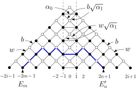
Figure 11. A graph designed so that the generating function for directed (from left to right) paths from $E_{m}$ (with coordinates $(-2m-1,0)$) to $E_{n}^{\prime}$ (with coordinates $(2n+1,0)$) precisely reproduces $F_{n+m}$ for quadrangulations.

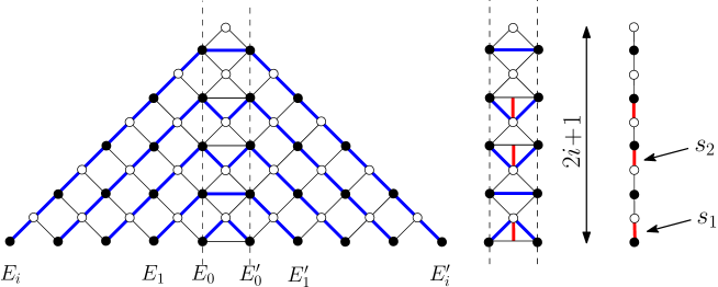
Figure 12. Mutually avoiding paths on the graph of Figure 11, from $E_{0},E_{1},\dots E_{i}$ to $E_{0}^{\prime},E_{1}^{\prime},\cdots E_{i}^{\prime}$. The only freedom comes from the central column (between abscissas $-1$ and $1$). The path configurations in this column are in one-to-one correspondence with hard dimers on a bicolored segment of length $2i+1$.

In the case of quadrangulations, we have

$$\begin{split}F_{n}^{\bullet}=&\alpha_{0}\hat{\mathbb{Z}}_{0,0}^{\bullet\bullet+}(2n)+\alpha_{1}\hat{\mathbb{Z}}_{0,0}^{\bullet\bullet+}(2n+2)\\ &\alpha_{0}=1+\frac{BW}{t_{\bullet}}\qquad\alpha_{1}=-\frac{B}{t_{\bullet}}\ .\\ \end{split}$$

The function $F_{m+n}$ may therefore be understood as the generating function for configurations of a directed (from left to right) path starting from point $E_{m}$ (with coordinates $(-2m-1,0)$) and ending at point $E_{n}^{\prime}$ (with coordinates $(2n+1,0)$), traveling on the graph of Figure 11, with appropriate edge weights designed so as to reproduce the above formula. More precisely, all diagonal edges used by the path receive a weight $b=\sqrt{B}$ or $w=\sqrt{W}$ respectively according to the white or black color of their lower vertex, except for the diagonal edges lying in the central vertical column (i.e., whose abscissas are between $-1$ and $1$), which receive instead a weight $b\sqrt{\alpha_{1}}$ or $w\sqrt{\alpha_{1}}$ (according again to the white or black color of their lower vertex). As for any horizontal edge used by the path in the central column, it gives rise instead to a weight $\alpha_{0}$. Now, from the LGV (Lindström-Gessel-Viennot) lemma, see for instance [13, 14], $h_{i}^{(0)}=\det_{0\leq m,n\leq i}F_{m+n}$ enumerates configurations of $i+1$ mutually avoiding directed paths with starting points $E_{0},\cdots E_{i}$ and endpoints $E_{0}^{\prime},\cdots,E_{i}^{\prime}$, see Figure 12. Because of the constraint of mutual avoidance, the parts of the paths lying outside the central column are entirely fixed, made only of ascending steps on the left side leading to black vertices with abscissa $-1$ and heights $0,2,\cdots,2i$ and made only of descending steps on the right side starting from black vertices with abscissa $1$ and heights $0,2,\cdots,2i$. The total weight of these portions of paths is $(BW)^{\frac{i(i+1)}{2}}$. As for the parts of the paths in the central column, they connect two black vertices of the same height (between $0$ and $2i$). This connection is done either via a horizontal edge, or via a sequence of two consecutive up/down or down/up diagonal edges. We may therefore decide to weigh the central column by $\alpha_{0}^{i+1}$ and to correct by a multiplicative weight $s_{1}=W(\alpha_{1}/\alpha_{0})$ for each used up/down sequence, and a multiplicative weight $s_{2}=B(\alpha_{1}/\alpha_{0})$ for each used down/up sequence. Note now that the mutual avoidance constraint prevents up/down and down/up portions to share a common white vertex, so that these portions repel each other and (by a simple vertical projection) act as hard dimers on a bicolored (vertical) oriented (from bottom to top) segment, see Figure 12.

More precisely, we call a bicolored oriented segment an oriented segment (i.e., a finite oriented linear graph) made of links whose nodes are bicolored alternatively in black and white. Each link of the segment may be occupied by a dimer or not, with the constraint that a node is incident to at most one dimer. Each dimer lying on a link oriented from a black to a white node receives the weight $s_{1}$ and each dimer lying on a link oriented from a white to a black node receives the weight $s_{2}$. We shall denote by $Z_{HD[0,2i]}^{\bullet\bullet}\equiv Z_{HD[0,2i]}^{\bullet\bullet}(s_{1},s_{2})$ the generating function of hard dimers on a bicolored oriented segment made of $2i$ links whose first and last nodes are black. We shall also use the notations $Z_{HD[0,2i]}^{\circ\circ}$, $Z_{HD[0,2i+1]}^{\bullet\circ}$ and $Z_{HD[0,2i+1]}^{\circ\bullet}$ for the other possible colors of the extremal nodes, with obvious definitions.

In the present case, the hard dimers configurations gathering the weights of the central column live on a segment of length $2i+1$ starting with a black node and ending with a white one, so that we may eventually write

$$\begin{split}&h_{i}^{(0)}=(BW)^{\frac{i(i+1)}{2}}\alpha_{0}^{i+1}Z_{HD[0,2i+1]}^{\bullet\circ}\\ &\hbox{with dimer weights}\ s_{1}=W\frac{\alpha_{1}}{\alpha_{0}}\qquad s_{2}=B\frac{\alpha_{1}}{\alpha_{0}}\ .\\ \end{split}$$

The generating functions $Z_{HD[0,2i]}^{\bullet\bullet}$, $Z_{HD[0,2i]}^{\circ\circ}$, $Z_{HD[0,2i+1]}^{\bullet\circ}$ and $Z_{HD[0,2i+1]}^{\circ\bullet}$ are computed in Appendix C. They are best expressed upon introducing the parametrization

$$s_{1}=-\frac{x}{(c+x)(1+c\,x)}\qquad s_{2}=-\frac{c^{2}x}{(c+x)(1+c\,x)}\ ,$$

which is achieved by taking

$$c=\sqrt{\frac{s_{2}}{s_{1}}}=\sqrt{\frac{B}{W}}\qquad x+\frac{1}{x}=-\frac{1+s_{1}+s_{2}}{c\,s_{1}}=-\frac{\frac{\alpha_{0}}{\alpha_{1}}+B+W}{\sqrt{BW}}\ .$$

The definition of $c$ matches precisely our definition of the general formalism. As for $x$, using (LABEL:eq:recurBWquad), we find that $(\alpha_{0}/\alpha_{1})+B+W=-(1-2(B+W))$ so that the above equation for $x$ matches precisely the characteristic equation (25). In terms of $x$ and $c$, we have (see Appendix C)

$$Z_{HD[0,2i+1]}^{\bullet\circ}=(1+c\,x)\left(\frac{c}{(c+x)(1+c\,x)}\right)^{i+1}\frac{1-\frac{c+x}{1+c\,x}x^{2i+3}}{1-x^{2}}\ .$$

so that

$$h_{i}^{(0)}=(BW)^{\frac{i(i+1)}{2}}\left(\frac{\alpha_{0}c}{(c+x)(1+c\,x)}\right)^{i+1}\frac{(1+c\,x)}{1-x^{2}}\left(1-\frac{c+x}{1+c\,x}x^{2i+3}\right)\ .$$

This is precisely the result (33) of our general formalism, since

$$\frac{\alpha_{0}c}{(c+x)(1+c\,x)}=\frac{\alpha_{0}}{x}\sqrt{s_{1}\,s_{2}}=\frac{\alpha_{0}}{x}\left(-\frac{\alpha_{1}}{\alpha_{0}}\right)\sqrt{BW}=\frac{B}{t_{\bullet}}\frac{\sqrt{BW}}{x}\ .$$

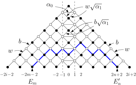
Figure 13. A graph designed so that the generating function for directed (from left to right) paths from $E_{m}$ (with coordinates $(-2m-2,0)$) to $E_{n}^{\prime}$ (with coordinates $(2n+2,0)$) precisely reproduces $F_{n+m+1}$ for quadrangulations.

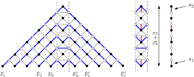
Figure 14. Mutually avoiding paths on the graph of Figure 13, from $E_{0},E_{1},\dots E_{i}$ to $E_{0}^{\prime},E_{1}^{\prime},\cdots E_{i}^{\prime}$. The only freedom comes from the central column (between abscissas $-1$ and $1$). The path configurations in this column are in one-to-one correspondence with hard dimers on a bicolored segment of length $2i+2$.

We may now play the same game to compute $h_{i}^{(1)}$ by interpreting the function $F_{m+n+1}$ as the generating function for configurations of a directed (from left to right) path starting from point $E_{m}$ (with coordinates $(-2m-2,0)$) and ending at point $E_{n}^{\prime}$ (with coordinates $(2n+2,0)$), traveling now on the graph of Figure 13, with the same weight prescription as before. From the LGV lemma, $h_{i}^{(1)}=\det_{0\leq m,n\leq i}F_{m+n+1}$ now enumerates configurations of $i+1$ mutually avoiding directed paths with starting points $E_{0},\cdots E_{i}$ and endpoints $E_{0}^{\prime},\cdots,E_{i}^{\prime}$, see Figure 14. The total weight of the (entirely fixed) portions of paths outside of the central column is now $W^{i+1}(BW)^{\frac{i(i+1)}{2}}$, while the contribution of the central column now reads $\alpha_{0}^{i+1}Z_{HD[0,2i+2]}^{\bullet\bullet}$, so that (see Appendix C for the formula for $Z_{HD[0,2i+2]}^{\bullet\bullet}$)

$$\begin{split}h_{i}^{(1)}&=W^{i+1}(BW)^{\frac{i(i+1)}{2}}\alpha_{0}^{i+1}Z_{HD[0,2i+2]}^{\bullet\bullet}\\ &=W^{i+1}(BW)^{\frac{i(i+1)}{2}}\left(\frac{\alpha_{0}c}{(c+x)(1+c\,x)}\right)^{i+1}\frac{1}{1-x^{2}}\left(1-x^{2i+4}\right)\end{split}$$

in agreement with the formula (24) of the general formalism. We leave as an exercise to the reader the care of computing $\tilde{h}_{i}^{(0)}$ and $\tilde{h}_{i}^{(1)}$ via the dimer formalism and checking that their expressions match the formulas of the general formalism.

6.2. The case of hexangulations

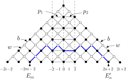
Figure 15. A graph designed so that the generating function for directed (from left to right) paths from $E_{m}$ (with coordinates $(-2m-2,0)$) to $E_{n}^{\prime}$ (with coordinates $(2n+2,0)$) precisely reproduces $F_{n+m}$ for hexangulations.

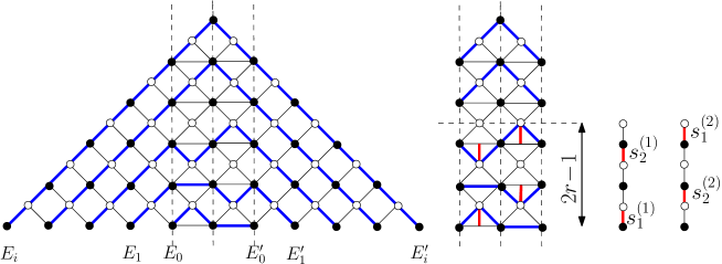
Figure 16. Mutually avoiding paths on the graph of Figure 15, from $E_{0},E_{1},\dots E_{i}$ to $E_{0}^{\prime},E_{1}^{\prime},\cdots E_{i}^{\prime}$. The only freedom comes from the two central columns (between abscissas $-2$ and $2$). The path configurations in these columns are in one-to-one correspondence with couples of two hard dimer configurations on bicolored segments of the same length $2r-1$, with $r$ ranging from $0$ to $i+1$ (by convention, the contribution of configurations with $r=0$ is taken to be $1$).

In the case of hexangulations, we have

$$\begin{split}F_{n}^{\bullet}=&\alpha_{0}\hat{\mathbb{Z}}_{0,0}^{\bullet\bullet+}(2n)+\alpha_{1}\hat{\mathbb{Z}}_{0,0}^{\bullet\bullet+}(2n+2)+\alpha_{2}\hat{\mathbb{Z}}_{0,0}^{\bullet\bullet+}(2n+4)\\ &\alpha_{0}=\frac{B}{t_{\bullet}}(1-L_{0}(4))=\frac{B}{t_{\bullet}}(1-B^{2}-W^{2}-4BW)\\ &\alpha_{1}=\frac{B}{t_{\bullet}}(-L_{0}(2))=-\frac{B}{t_{\bullet}}(B+W)\\ &\alpha_{2}=\frac{B}{t_{\bullet}}(-L_{0}(0))=-\frac{B}{t_{\bullet}}\ .\\ \end{split}$$

To compute $h_{i}^{(0)}$, we shall here use a slightly different strategy from that used for quadrangulations, i.e., look at the function $F_{m+n}/\alpha_{2}$. The function $F_{m+n}/\alpha_{2}$ is indeed the generating function for configurations of a directed (from left to right) path starting from point $E_{m}$ (with coordinates $(-2m-2,0)$) and ending at point $E_{n}^{\prime}$ (with coordinates $(2n+2,0)$), traveling on the graph of Figure 15, with the following appropriate edge weights: all diagonal edges used by the path receive a weight $b=\sqrt{B}$ or $w=\sqrt{W}$ respectively according to the white or black color of their lower vertex, including those diagonal edges lying in the two central vertical columns (i.e., whose abscissas are between $-2$ and $2$). As for any horizontal edge used by the path in the two central columns, they give rise instead to a weight $p_{1}$ for the first central column (with abscissas between $-2$ and $0$) and $p_{2}$ in the second central column (with abscissas between $0$ and $2$), with

$$p_{1}+p_{2}=\frac{\alpha_{1}}{\alpha_{2}}=B+W\qquad p_{1}p_{2}=\frac{\alpha_{0}}{\alpha_{2}}=B^{2}+W^{2}+4BW-1\ .$$

Indeed, with these weights, the set of those paths using no horizontal edge indeed contributes $\hat{\mathbb{Z}}_{0,0}^{\bullet\bullet+}(2m+2n+4)$, that of those paths using one horizontal edge contributes $(\alpha_{1}/\alpha_{2})\hat{\mathbb{Z}}_{0,0}^{\bullet\bullet+}(2m+2n+2)$ and that of those paths using two horizontal edges contributes $(\alpha_{0}/\alpha_{2})\hat{\mathbb{Z}}_{0,0}^{\bullet\bullet+}(2m+2n)$. As before, $h_{i}^{(0)}/\alpha_{2}^{i+1}$ enumerates mutually avoiding paths with starting points $E_{0},\cdots E_{i}$ and endpoints $E_{0}^{\prime},\cdots,E_{i}^{\prime}$, see Figure 16. Again the parts of the paths lying outside the two central columns is entirely fixed, made only of ascending steps on the left side leading to black vertices with abscissa $-2$ and heights $0,2,\cdots,2i$ and made only of descending steps on the right side starting from black vertices with abscissa $2$ and heights $0,2,\cdots,2i$. The total weight of these portions of paths is again $(BW)^{\frac{i(i+1)}{2}}$. The parts of the paths in the two central columns connect two black vertices of the same height (between $0$ and $2i$) and it is interesting to classify these paths according to the position of their passage at abscissa $0$ (i.e., at the contact of the two central columns). Due to the mutual avoidance constraint, the corresponding heights are $0,2,\cdots,2r-2$ for the lower $r$ paths and $2r+2,2r+4,\cdots 2i+2$ for the higher $i+1-r$ paths, with $r$ some integer ranging from $0$ to $i+1$, see Figure 16. The last higher $i+1-r$ paths contribute $(BW)^{i+1-r}$ while the $r$ first ones contribute $(p_{1})^{r}Z_{HD[0,2r-1]}^{\bullet\circ}(s_{1}^{(1)},s_{2}^{(1)})$ (from the first central column) and $(p_{2})^{r}Z_{HD[0,2r-1]}^{\bullet\circ}(s_{1}^{(2)},s_{2}^{(2)})$ (from the second central column) with

$$s_{1}^{(1)}=\frac{W}{p_{1}}\qquad s_{2}^{(1)}=\frac{B}{p_{1}}\qquad s_{1}^{(2)}=\frac{W}{p_{2}}\qquad s_{2}^{(2)}=\frac{B}{p_{2}}$$

and the convention $Z_{HD[0,-1]}^{\bullet\bullet}=1$. This leads to the formula

(36) $$\frac{h_{i}^{(0)}}{\alpha_{2}^{i+1}}=(BW)^{\frac{i(i+1)}{2}}\sum_{r=0}^{i+1}(BW)^{i+1-r}(p_{1}p_{2})^{r}Z_{HD[0,2r-1]}^{\bullet\circ}(s_{1}^{(1)},s_{2}^{(1)})Z_{HD[0,2r-1]}^{\bullet\circ}(s_{1}^{(2)},s_{2}^{(2)})\ .$$

Using the parametrization

$$\begin{split}&s_{1}^{(1)}=\frac{W}{p_{1}}=-\frac{x_{1}}{(c+x_{1})(1+c\,x_{1})}\qquad s_{2}^{(1)}=\frac{B}{p_{1}}=-\frac{c^{2}x_{1}}{(c+x_{1})(1+c\,x_{1})}\\ &s_{1}^{(2)}=\frac{W}{p_{2}}=-\frac{x_{2}}{(c+x_{2})(1+c\,x_{2})}\qquad s_{2}^{(2)}=\frac{B}{p_{2}}=-\frac{c^{2}x_{2}}{(c+x_{2})(1+c\,x_{1})}\\ \end{split}$$

by setting

$$\begin{split}&c=\sqrt{\frac{s_{2}^{(1)}}{s_{1}^{(1)}}}=\sqrt{\frac{s_{2}^{(2)}}{s_{1}^{(2)}}}=\sqrt{\frac{B}{W}}\\ &x_{1}+\frac{1}{x_{1}}=-\frac{1+s_{1}^{(1)}+s_{2}^{(1)}}{c\,s_{1}^{(1)}}=-\frac{p_{1}+B+W}{\sqrt{BW}}\\ &x_{2}+\frac{1}{x_{2}}=-\frac{1+s_{1}^{(2)}+s_{2}^{(2)}}{c\,s_{1}^{(2)}}=-\frac{p_{2}+B+W}{\sqrt{BW}}\ ,\\ \end{split}$$

we can use our general formula for $Z_{HD[0,2r-1]}^{\bullet\circ}$ and write for instance

$$\begin{split}(p_{1})^{r}Z_{HD[0,2r-1]}^{\bullet\circ}(s_{1}^{(1)},s_{2}^{(1)})&=(1+c\,x_{1})\left(\frac{p_{1}c}{(c+x_{1})(1+c\,x_{1})}\right)^{r}\frac{1-\frac{c+x_{1}}{1+c\,x_{1}}x_{1}^{2r+1}}{1-x_{1}^{2}}\\ &=(1+c\,x_{1})\left(\frac{\sqrt{BW}}{x_{1}}\right)^{r}\frac{1-\frac{c+x_{1}}{1+c\,x_{1}}x_{1}^{2r+1}}{1-x_{1}^{2}}\\ \end{split}$$

(note that the formula also holds for $r=0$ with our convention $Z_{HD[0,-1]}^{\bullet\bullet}=1$). Eq. (36) yields

$$h_{i}^{(0)}=\alpha_{2}^{i+1}(BW)^{\frac{(i+1)(i+2)}{2}}\frac{1+c\,x_{1}}{1-x_{1}^{2}}\frac{1+c\,x_{2}}{1-x_{2}^{2}}\sum_{r=0}^{i+1}(x_{1}^{-r}-\frac{c+x_{1}}{1+c\,x_{1}}x_{1}^{r+1})(x_{2}^{-r}-\frac{c+x_{2}}{1+c\,x_{2}}x_{2}^{r+1})\ .$$

The sum over $r$ is easily performed and we end up with the desired result

$$h_{i}^{(0)}=\alpha_{2}^{i+1}(BW)^{\frac{(i+1)(i+2)}{2}}\frac{1}{(x_{1}x_{2})^{i+1}}\frac{1+c\,x_{1}}{1-x_{1}^{2}}\frac{1+c\,x_{2}}{1-x_{2}^{2}}\frac{1}{1-x_{1}x_{2}}\,\bar{u}_{2i+3}$$

with $\bar{u}_{i}$ as in eq. (34). For a full check of consistency, we still need to verify that $x_{1}$ and $x_{2}$ are the solutions of the correct characteristic equation (27). From their definition, $p_{1}$ and $p_{2}$ are solutions of the equation

$$0=p^{2}-\frac{\alpha_{1}}{\alpha_{2}}p+\frac{\alpha_{0}}{\alpha_{2}}=p^{2}-(B+W)p-1+B^{2}+W^{2}+4BW$$

so that $x_{1}$ and $x_{2}$ are solutions of

$$\begin{split}0=&\left(-(B+W)-\sqrt{BW}\left(x+\frac{1}{x}\right)\right)^{2}-(B+W)\left(-(B+W)-\sqrt{BW}\left(x+\frac{1}{x}\right)\right)\\ &\hskip 227.62204pt-1+B^{2}+W^{2}+4BW\\ \end{split}$$

which after simplification precisely reproduces (27).

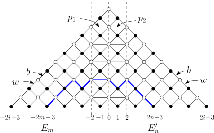
Figure 17. A graph designed so that the generating function for directed (from left to right) paths from $E_{m}$ (with coordinates $(-2m-3,0)$) to $E_{n}^{\prime}$ (with coordinates $(2n+3,0)$) precisely reproduces $F_{n+m+1}$ for hexangulations.

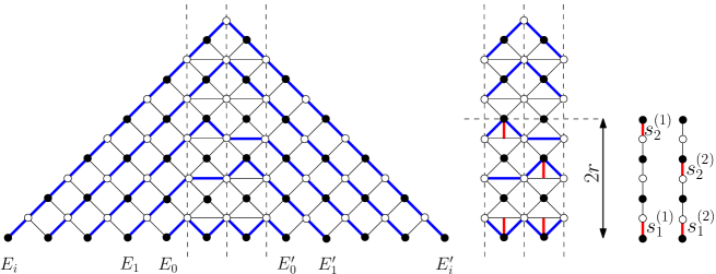
Figure 18. Mutually avoiding paths on the graph of Figure 17, from $E_{0},E_{1},\dots E_{i}$ to $E_{0}^{\prime},E_{1}^{\prime},\cdots E_{i}^{\prime}$. The only freedom comes from the two central columns (between abscissas $-2$ and $2$). The path configurations in these columns are in one-to-one correspondence with pairs of two hard dimer configurations on bicolored segments of the same length $2r$, with $r$ ranging from $0$ to $i+1$.

If we now wish to play the same game to compute $h_{i}^{(1)}$, we interprete $F_{m+n+1}$ as the generating function for configurations of a directed path starting from point $E_{m}$ (with coordinates $(-2m-3,0)$) and ending at point $E_{n}^{\prime}$ (with coordinates $(2n+3,0)$) traveling on the graph of Figure 17, with the same weight prescription as before. Then $h_{i}^{(1)}/\alpha_{2}^{i+1}$ enumerates mutually avoiding paths with starting points $E_{0},\cdots E_{i}$ and endpoints $E_{0}^{\prime},\cdots,E_{i}^{\prime}$, see Figure 18, and we now obtain

$$\frac{h_{i}^{(1)}}{\alpha_{2}^{i+1}}=W^{i+1}(BW)^{\frac{i(i+1)}{2}}\sum_{r=0}^{i+1}(BW)^{i+1-r}(p_{1}p_{2})^{r}Z_{HD[0,2r]}^{\bullet\bullet}(s_{1}^{(1)},s_{2}^{(1)})Z_{HD[0,2r]}^{\bullet\bullet}(s_{1}^{(2)},s_{2}^{(2)})$$

which yields

$$h_{i}^{(1)}=\alpha_{2}^{i+1}W^{i+1}(BW)^{\frac{(i+1)(i+2)}{2}}\frac{1}{1-x_{1}^{2}}\frac{1}{1-x_{2}^{2}}\sum_{r=0}^{i+1}(x_{1}^{-r}-x_{1}^{r+2})(x_{2}^{-r}-x_{2}^{r+2})$$

and, after summation over $r$

$$h_{i}^{(1)}=\alpha_{2}^{i+1}W^{i+1}(BW)^{\frac{(i+1)(i+2)}{2}}\frac{1}{(x_{1}x_{2})^{i+1}}\frac{1}{1-x_{1}^{2}}\frac{1}{1-x_{2}^{2}}\frac{1}{1-x_{1}x_{2}}\,u_{2i+4}$$

with $u_{i}$ as in eq. (26). We again leave as an exercise to the reader the care of computing $\tilde{h}_{i}^{(0)}$ and $\tilde{h}_{i}^{(1)}$ via the dimer formalism and checking that their expressions match the formulas of general formalism.

7. Conclusion

In this paper, we obtained expressions for the two-point function of bicolored maps, with a control on their (even) face degrees and on their numbers of black and white vertices (via the weights $t_{\bullet}$ and $t_{\circ}$), in the form of explicit formulas for the corresponding black or white $i$-slice generating functions. For maps with faces of degrees at most $2p+2$, these formulas take the form of ratios of $p\times p$ determinants, generalizing those found in [8] in the uncolored version of the problem. In the simplest case of bicolored quadrangulations ($p=1$) and hexangulations ($p=2$), the very same formulas may be recovered via an equivalence with appropriate hard dimer problems on segments, with parity dependent weights.

Let us now discuss a few extensions of our results. First, starting from generating functions for our families of maps, we can in some cases, by a simple substitution, get generating functions for other families of maps, incorporating additional restrictions (such as the absence of multiple edges, ….). Such substitutions are particularly useful in the context of irreducible maps (with a control on the length of their smallest cycles) and, as shown in [9], the required substitution may then be determined so as to give (after substitution) trivial values (such as $1$ or so) to the first conserved quantities (which are non-trivial in the original problem). This in turn provides a way to construct new equations which essentially have the same solution as the original ones, up to a redefinition of the weights, see [9]. We can play this game starting, say, from our solution of bicolored quadrangulations to derive new sets of integrable equations, with explicit solutions.

Another extension deals with the case of $p$-constellations for $p>2$. Recall that a $p$-constellation is a face-bicolored map (say with dark and light faces) such that all dark faces have degree $p$ and all light faces have a degree multiple of $p$. In the planar case, we may naturally color the vertices of these maps in $p$ colors in increasing (resp. decreasing) order clockwise around the black (resp. the white faces). Our bicolored maps are nothing but $2$-constellations (where the dark faces – of degree $2$ – have been squeezed into edges) and we may try to extend our results to $p$-constellations with $p>2$, giving different weights to the vertices, according to their color. We discuss below an example with $p=3$.

7.1. Other integrable equations from the solution of bicolored quadrangulations

Using the conserved quantities (15) for bicolored quadrangulations, the corresponding $B_{i}$’s and $W_{i}$’s may alternatively be viewed as the solutions of

$$\begin{split}&F_{1}^{\bullet}=W_{i}-\frac{1}{t_{\bullet}}B_{i-1}W_{i}B_{i+1}=W_{1}\\ &F_{1}^{\circ}=B_{i}-\frac{1}{t_{\circ}}W_{i-1}B_{i}W_{i+1}=B_{1}\\ \end{split}$$

for $i\geq 1$ with $B_{0}=W_{0}=0$. Note that these equations are however weaker than the original system as they do not determine in practice $B_{1}$ and $W_{1}$, nor $B$ and $W$ but only the relations $B_{1}=B(1-W^{2}/t_{\circ})$ and $W_{1}=W(1-B^{2}/t_{\bullet})$ (while the original equations fix $B$ and $W$ via $t_{\bullet}=B(1-2W-B)$ and $t_{\circ}=W(1-2B-W)$, and the values of $B_{1}$ and $W_{1}$ follow). We may in practice eliminate $B_{1}$ and $W_{1}$ upon defining

$$P_{i}=\frac{B_{i}}{B_{1}}\qquad Q_{i}=\frac{W_{i}}{W_{1}}$$

for $i\geq 0$. We indeed get for $P_{i}$ and $W_{i}$ the system of equations

(37) $$\begin{split}&P_{i}=1+z_{\circ}Q_{i-1}P_{i}Q_{i+1}\\ &Q_{i}=1+z_{\bullet}P_{i-1}Q_{i}P_{i+1}\\ \end{split}$$

valid for $i\geq 1$, with initial conditions $P_{0}=Q_{0}=0$, and with

$$z_{\circ}=\frac{W_{1}^{2}}{t_{\circ}}\qquad z_{\bullet}=\frac{B_{1}^{2}}{t_{\bullet}}\ .$$

We may in practice forget about these latter relations and consider $z_{\bullet}$ and $z_{\circ}$ as our new input. Note that $P_{1}=Q_{1}$ are now determined, with value $1$. We immediately deduce from (35) the solution of (37)

$$\begin{split}&P_{2i}=P\frac{u_{2i}\bar{u}_{2i+3}}{\bar{u}_{2i+1}u_{2i+2}}\qquad Q_{2i+1}=Q\frac{\bar{u}_{2i+1}u_{2i+4}}{u_{2i+2}\bar{u}_{2i+3}}\\ &P_{2i+1}=P\frac{\hat{u}_{2i+1}u_{2i+4}}{u_{2i+2}\hat{u}_{2i+3}}\qquad Q_{2i}=Q\frac{u_{2i}\hat{u}_{2i+3}}{\hat{u}_{2i+1}u_{2i+2}}\\ \end{split}$$

where $P\equiv B/B_{1}$ and $Q\equiv W/W_{1}$ are the solutions of

$$\begin{split}&P=1+z_{\circ}Q^{2}P\\ &Q=1+z_{\bullet}P^{2}Q\ ,\\ \end{split}$$

and $u_{i}$, $\bar{u}_{i}$ and $\hat{u}_{i}$ have the same definitions as before in terms of $x$ and $c$. As for $c$ and $x$ themselves, they can be related directly to $P$ and $Q$ via

$$c=\sqrt{\frac{Q-1}{P-1}}\ ,\qquad\left(x+\frac{1}{x}\right)\sqrt{(P-1)(Q-1)}=1\ .$$

These equations are easily obtained by rewriting $B$ and $W$ in terms of $P$ and $Q$. Using $(P-1)/(Q^{2}P)=z_{\circ}=W_{1}^{2}/t_{\circ}=(W/Q)^{2}/t_{\circ}$ and, from (LABEL:eq:recurBWquad), the relation $t_{\circ}=W(1-2B-W)$, we get $(P-1)=W/(1-2B-2W)$ and, similarly, $(Q-1)=B/(1-2B-2W)$ so that $B/W=(Q-1)/(P-1)$, while (25) immediately yields the above equation for $x$. Alternatively, both equations may be obtained directly without recourse to neither (LABEL:eq:recurBWquad) nor (25) upon simply writing $P_{1}=Q_{1}=1$ and, using their explicit expressions above $P_{1}=P(\hat{u}_{1}u_{4})/(u_{2}\hat{u}_{3})$ and $Q_{1}=Q(\bar{u}_{1}u_{4})/(u_{2}\bar{u}_{3})$, solving for $c$ and $x$.

From the form of (37), we can immediately interpret $P_{i}$ and $Q_{i}$ as generating functions for naturally embedded ternary trees in a semi-infinite line, i.e., ternary trees whose vertices occupy positive integer positions on a line and where each internal vertex at position $j$ has its three children at positions $j-1$, $j$ and $j+1$ respectively. Such trees start with a univalent (uncolored) root vertex and have their internal vertices bicolored in black and white according to the parity of their position, and weighted by $z_{\bullet}$ and $z_{\circ}$ accordingly. More precisely (up to a first trivial term $1$ corresponding to the tree without internal vertices), $P_{i}$ corresponds to trees with a first internal vertex (i.e., that attached to the univalent root vertex) being at position $i$ and where each internal vertex whose position has the same parity as $i$ (resp. a different parity) is white (resp. black), while $Q_{i}$ corresponds to a first internal vertex at position $i$ with each internal vertex whose position has the same parity as $i$ (resp. a different parity) being black (resp. white). Naturally embedded ternary trees in a semi-infinite line are known to appear in the context of quadrangulations without multiple edges (which also correspond to nonseparable planar maps) [7, 9, 15], and the above generating functions would naturally appear in the bicolored version of this problem.

We may go one step further by using the next conserved quantities for bicolored quadrangulations, given (according to (14) with $d=i-1$) by

$$\begin{split}&F_{2}^{\bullet}=W_{i}(W_{i}+B_{i+1})-\frac{1}{t_{\bullet}}(W_{i}+B_{i+1}+W_{i+2})B_{i-1}W_{i}B_{i+1}=W_{1}(W_{1}+B_{2})\\ &F_{2}^{\circ}=B_{i}(B_{i}+W_{i+1})-\frac{1}{t_{\circ}}(B_{i}+W_{i+1}+B_{i+2})W_{i-1}B_{i}W_{i+1}=B_{1}(B_{1}+W_{2})\\ \end{split}$$

for $i\geq 1$ with $B_{0}=W_{0}=0$. Dividing the first equation by $t_{\circ}$ and the second by $t_{\bullet}$, we get alternatively

$$\begin{split}&\frac{F_{2}^{\bullet}}{t_{\circ}}=Q_{i}(z_{\circ}Q_{i}+z_{\bullet}P_{i+1})-z_{\bullet}(z_{\circ}P_{i}+z_{\bullet}P_{i+1}+z_{\circ}Q_{i+2})P_{i-1}Q_{i}P_{i+1}=(z_{\circ}+z_{\bullet}P_{2})\\ &\frac{F_{2}^{\circ}}{t_{\bullet}}=P_{i}(z_{\bullet}P_{i}+z_{\circ}Q_{i+1})-z_{\circ}(z_{\bullet}P_{i}+z_{\circ}Q_{i+1}+z_{\bullet}P_{i+2})Q_{i-1}P_{i}Q_{i+1}=(z_{\bullet}+z_{\circ}Q_{2})\ ,\\ \end{split}$$

a system which however does not determine $P_{2}$ and $Q_{2}$. Let us recall that, from (1), $F_{2}^{\bullet}/t_{\circ}=F_{2}^{\circ}/t_{\bullet}$ so that both lines in the above system are in practice equal. In particular, $(z_{\circ}+z_{\bullet}P_{2})=(z_{\bullet}+z_{\circ}Q_{2})$, so we can define

$$\delta=\frac{Q_{2}-1}{z_{\bullet}}=\frac{P_{2}-1}{z_{\circ}}\ .$$

Using $z_{\circ}Q_{i-1}P_{i}Q_{i+1}=P_{i}-1$ and $z_{\bullet}P_{i-1}Q_{i}P_{i+1}=Q_{i}-1$, this system simplifies into

$$\begin{split}&z_{\bullet}P_{i+1}+z_{\circ}(Q_{i}+Q_{i+2}-Q_{i}Q_{i+2})=z_{\bullet}+z_{\circ}+z_{\bullet}z_{\circ}\delta\\ &z_{\circ}Q_{i+1}+z_{\bullet}(P_{i}+P_{i+2}-P_{i}P_{i+2})=z_{\circ}+z_{\bullet}+z_{\circ}z_{\bullet}\delta\ .\\ \end{split}$$

Upon setting

$$R_{i}=\frac{P_{i+1}-1}{z_{\circ}\delta}\ ,\qquad S_{i}=\frac{Q_{i+1}-1}{z_{\bullet}\delta}\ ,$$

the system becomes

(38) $$\begin{split}&R_{i}=1+y_{\bullet}S_{i-1}S_{i+1}\\ &S_{i}=1+y_{\circ}R_{i-1}R_{i+1}\\ \end{split}$$

valid for $i\geq 1$ with $R_{0}=S_{0}=0$ (so that $R_{1}=S_{1}=1$), where we have set:

$$y_{\bullet}=z_{\bullet}\delta\ ,\qquad y_{\circ}=z_{\circ}\delta\ .$$

Again we may forget about $z_{\bullet}$ and $z_{\circ}$ and consider $y_{\bullet}$ and $y_{\circ}$ as our new input (the above change of functions being a way to get rid of the undetermined $P_{2}$ and $Q_{2}$). Introducing $R=(P-1)/(z_{\circ}\delta)$ and $S=(Q-1)/(z_{\bullet}\delta)$, determined by the system:

$$R=1+y_{\bullet}S^{2}\ ,\qquad S=1+y_{\circ}R^{2}\ ,$$

and using the equations for $P_{i}$ and $Q_{i}$ to write $R_{i}=Q_{i}P_{i+1}Q_{i+2}/\delta$ and $S_{i}=P_{i}Q_{i+1}P_{i+2}/\delta$ (and, accordingly, $R=Q^{2}P/\delta$ and $S=P^{2}Q/\delta$), we eventually get

$$\begin{split}&R_{2i}=R\frac{u_{2i}\hat{u}_{2i+5}}{u_{2i+2}\hat{u}_{2i+3}}\qquad S_{2i+1}=S\frac{\hat{u}_{2i+1}u_{2i+6}}{\hat{u}_{2i+3}u_{2i+4}}\\ &R_{2i+1}=R\frac{\bar{u}_{2i+1}u_{2i+6}}{\bar{u}_{2i+3}u_{2i+4}}\qquad S_{2i}=S\frac{u_{2i}\bar{u}_{2i+5}}{u_{2i+2}\bar{u}_{2i+3}}\ .\\ \end{split}$$

As for $c$ and $x$, they are now related to $R$ and $S$ via

$$c=\sqrt{\frac{R(R-1)}{S(S-1)}}\ ,\qquad\left(x+\frac{1}{x}\right)\sqrt{\frac{(R-1)(S-1)}{RS}}=1\ .$$

These equations are obtained by writing $(P-1)=z_{\circ}\delta R=y_{\circ}R=(S-1)/R$ and, similarly, $(Q-1)=(R-1)/S$. As before, both equations may alternatively be obtained by simply writing $R_{1}=S_{1}=1$ with their general expressions above, and solving for $c$ and $x$.

From the form of (38), we can immediately interpret $R_{i}$ and $S_{i}$ as generating functions for bicolored naturally embedded binary trees in a semi-infinite line with black and white internal vertex weights $y_{\bullet}$ and $y_{\circ}$. Such (uncolored) trees appear in the context of irreducible quadrangulations [9], and the above generating functions would therefore appear naturally in the bicolored version of this problem.

7.2. An integrable system with $3$ colors

Another remarkable system of equations which may be solved is

$$\begin{split}&T_{i}=t_{\bullet}+T_{i}(U_{i-1}+V_{i+1})\\ &U_{i}=t_{\circ}+U_{i}(V_{i-1}+T_{i+1})\\ &V_{i}=t_{\o}+V_{i}(T_{i-1}+U_{i+1})\\ \end{split}$$

for $i\geq 1$, with $T_{0}=U_{0}=V_{0}=0$. For $t_{\bullet}=t_{\circ}=t_{\o}$, we have $T_{i}=U_{i}=V_{i}$ and the three equations are the same. This common equation appears in the context of Eulerian triangulations [4] which are the simplest example of $3$-constellations. These maps are naturally divided into $3$ sublattices and the above system corresponds to giving a different weight to the vertices according to which sublattice they belong to. Introducing the solutions $T,U,V$ of

$$T=t_{\bullet}+T(U+V)\,\qquad U=t_{\circ}+U(V+T)\,\qquad V=t_{\o}+V(T+U)\ ,$$

the solution now depends on the congruence modulo $3$ of $i$. We find, for $i\geq 0$:

$$\begin{split}&T_{3i}=T\frac{(1\!-\!x^{3i})(1\!-\!\alpha x^{3i+4})}{(1\!-\!\alpha x^{3i+1})(1\!-\!x^{3i+3})}\quad T_{3i+1}=T\frac{(1\!-\!\gamma x^{3i+1})(1\!-\!x^{3i+5}/\epsilon)}{(1\!-\!x^{3i+2}/\epsilon)(1\!-\!\gamma x^{3i+4})}\quad T_{3i+2}=T\frac{(1\!-\!x^{3i+2}/\alpha)(1\!-\!x^{3i+6})}{(1\!-\!x^{3i+3})(1\!-\!x^{3i+5}/\alpha)}\\ &U_{3i}=U\frac{(1\!-\!x^{3i})(1\!-\!\gamma x^{3i+4})}{(1\!-\!\gamma x^{3i+1})(1\!-\!x^{3i+3})}\quad U_{3i+1}=U\frac{(1\!-\!\epsilon x^{3i+1})(1\!-\!x^{3i+5}/\alpha)}{(1\!-\!x^{3i+2}/\alpha)(1\!-\!\epsilon x^{3i+4})}\quad U_{3i+2}=U\frac{(1\!-\!x^{3i+2}/\gamma)(1\!-\!x^{3i+6})}{(1\!-\!x^{3i+3})(1\!-\!x^{3i+5}/\gamma)}\\ &V_{3i}=V\frac{(1\!-\!x^{3i})(1\!-\!\epsilon x^{3i+4})}{(1\!-\!\epsilon x^{3i+1})(1\!-\!x^{3i+3})}\quad V_{3i+1}=V\frac{(1\!-\!\alpha x^{3i+1})(1\!-\!x^{3i+5}/\gamma)}{(1\!-\!x^{3i+2}/\gamma)(1\!-\!\alpha x^{3i+4})}\quad V_{3i+2}=V\frac{(1\!-\!x^{3i+2}/\epsilon)(1\!-\!x^{3i+6})}{(1\!-\!x^{3i+3})(1\!-\!x^{3i+5}/\epsilon)}\ .\\ \end{split}$$

Here $\alpha,\gamma$ and $\epsilon$ are expressed in terms of four quantities $t,u,v$ and $x$ only via

$$\alpha=\frac{v+u\,x+t\,x^{2}}{t+v\,x+u\,x^{2}}\qquad\gamma=\frac{t+v\,x+u\,x^{2}}{u+t\,x+v\,x^{2}}\qquad\epsilon=\frac{u+t\,x+v\,x^{2}}{v+u\,x+t\,x^{2}}$$

(note that $\alpha\gamma\epsilon=1$ and that these three quantities depend in practice only on the three quantities $x$, $u/t$ and $v/t$ so that we could therefore set $t=1$ without loss of generality). As for the quantities $t,u,v$ and $x$ themselves, they are obtained from $U,V$ and $T$ via

$$T=\frac{u\,v\,x}{(u+t\,x)(t+v\,x)}\qquad U=\frac{t\,v\,x}{(u+t\,x)(v+u\,x)}\qquad V=\frac{t\,u\,x}{(v+u\,x)(t+v\,x)}$$

(again these three equations determine only $x$ and the ratios $u/t$ and $v/t$, which is all what we need in practice). With these expressions, it is easy to check that $x$ satisfies the characteristic equation

$$TUV\left(x^{3}+\frac{1}{x^{3}}+2\right)-(1-T-U-V)^{2}=0$$

(note that if $x$ is a solution, $\omega x$ and $\omega^{2}x$, with $\omega=e^{2i\pi/3}$ are also solutions, as well as their inverses. The precise determination of $x$ is in practice irrelevant, for instance changing $x\to\omega x$ will result into $t\to t$, $u\to\omega u$, $v\to\omega^{2}v$, and then $\alpha\to\omega^{2}\alpha$, $\gamma\to\omega^{2}\gamma$ and $\epsilon\to\omega^{2}\epsilon$ so that the expressions for $T_{i}$, $U_{i}$ and $V_{i}$ remain the same). The solution above was obtained by simple guessing. It should in principle be possible to obtain it in a constructive way via the formalism of multicontinued fractions developed in [1].

Let us finally mention that one can extract trivariate series expansions from these expressions, similarly as was done in Section 5. Defining $u^{\prime}\equiv u/t$, $v^{\prime}\equiv v/t$, the parametrization of $T,U,V$ in terms of $t,u,v,x$ is equivalent to the system

$$1=U\left(1+\frac{u^{\prime}}{x}\right)+V(1+v^{\prime}x),\quad u^{\prime}=V\left(u^{\prime}+\frac{v^{\prime}}{x}\right)+T(u^{\prime}+x),\quad v^{\prime}=T\left(v^{\prime}+\frac{1}{x}\right)+U(v^{\prime}+u^{\prime}x)\ .$$

Defining $y\equiv x^{3}$, $d\equiv u^{\prime}x^{2}$, $e\equiv v^{\prime}x$, this rewrites as

$$y=U(y+d)+Vy(1+e),\quad d=V(d+e)+T(d+y),\quad e=T(e+1)+U(e+d)$$

so that $y,e,d$ have (positive) series expansions in $\{T,U,V\}$, and thus also (positive) series expansions in $\{t_{\bullet},t_{\circ},t_{\o}\}$. Then the expressions of $T_{i},U_{i},V_{i}$ above can in all cases be rewritten as rational expressions in terms of $d,e,y$, thereby well suited for series expansions. For instance

$$T_{3i}=T\frac{(1-y^{i})(1-\hat{\alpha}y^{i+1})}{(1-\hat{\alpha}y^{i})(1-y^{i+1})},\ \mathrm{where}\ \hat{\alpha}=x\alpha=\frac{e+d+y}{1+e+d}\ .$$

Appendix A Direct approaches for quadrangulations

A.1. Using conserved quantities

A direct expression for $B_{i}$ and $W_{i}$ can be obtained for quadrangulations by simply using the conserved quantities

(39) $$\begin{split}c_{i}&=B_{i+1}-\frac{1}{t_{\circ}}W_{i}B_{i+1}W_{i+2}\\ \tilde{c}_{i}&=W_{i+1}-\frac{1}{t_{\bullet}}B_{i}W_{i+i}B_{i+2}\\ \end{split}$$

which don’t depend on $i$ for all $i\geq 0$. If we look for $B_{i}$ and $W_{i}$ in the form

$$\begin{split}&B_{2i}=B\frac{u_{2i}\bar{u}_{2i+3}}{\bar{u}_{2i+1}u_{2i+2}}\qquad W_{2i+1}=W\frac{\bar{u}_{2i+1}u_{2i+4}}{u_{2i+2}\bar{u}_{2i+3}}\\ &B_{2i+1}=B\frac{\hat{u}_{2i+1}u_{2i+4}}{u_{2i+2}\hat{u}_{2i+3}}\qquad W_{2i}=W\frac{u_{2i}\hat{u}_{2i+3}}{\hat{u}_{2i+1}u_{2i+2}}\\ \end{split}$$

for some unknown functions $u_{i}$, $\bar{u}_{i}$ and $\hat{u}_{i}$, writing $c_{2i-1}=B-\frac{1}{t_{\circ}}W^{2}B$ and $\tilde{c}_{2i}=W-\frac{1}{t_{\bullet}}B^{2}W$ yields the two equations

$$\begin{split}&B(\bar{u}_{2i+3}u_{2i}-\bar{u}_{2i+1}u_{2i+2})-\frac{1}{t_{\circ}}W^{2}B(\bar{u}_{2i-1}u_{2i+4}-\bar{u}_{2i+1}u_{2i+2})=0\\ &W(\bar{u}_{2i+1}u_{2i+4}-\bar{u}_{2i+3}u_{2i+2})-\frac{1}{t_{\bullet}}B^{2}W(\bar{u}_{2i+5}u_{2i}-\bar{u}_{2i+3}u_{2i+2})=0\ .\\ \end{split}$$

Taking now

$$u_{2i}=1-\lambda\,x^{2i}\qquad\bar{u}_{2i+1}=1-\mu\,x^{2i+1}\ ,$$

we see that the constant term (i.e., the term independent of $\lambda$ and $\mu$) clearly vanishes in both equations as well as the term proportional to $\lambda\mu$ since, in both equations, the sum of the indices is the same (respectively $4i+3$ and $4i+5$) in all $\bar{u}\,u$ terms. As for the linear terms in $\lambda$ and $\mu$, their vanishing implies

$$\begin{split}&B(\mu x^{3}+\lambda-\mu x-\lambda x^{2})-\frac{1}{t_{\circ}}W^{2}B(\mu x^{-1}+\lambda x^{4}-\mu x-\lambda x^{2})=0\\ &W(\mu x+\lambda x^{4}-\mu x^{3}-\lambda x^{2})-\frac{1}{t_{\bullet}}B^{2}W(\mu x^{5}+\lambda-\mu x^{3}-\lambda x^{2})=0\ .\\ \end{split}$$

Now, imposing $B_{0}=W_{0}$ leads us to choose $\lambda=1$. Eliminating $\mu$ from the above system yields then the equation for $x$:

$$B^{2}W^{2}\left(x^{2}+\frac{1}{x^{2}}+1\right)+t_{\circ}B^{2}+t_{\bullet}W^{2}-t_{\bullet}t_{\circ}=0$$

while $\mu$ is obtained for instance via

$$\mu=x\,\frac{t_{\circ}+W^{2}x^{2}}{W^{2}+t_{\circ}x^{2}}\ .$$

After writing $t_{\bullet}=B(1-2W-B)$ and $t_{\circ}=W(1-2B-W)$, the equation for $x$ factors into

$$\left(1-2(B+W)-\sqrt{BW}\left(x+\frac{1}{x}\right)\right)\left(1-2(B+W)+\sqrt{BW}\left(x+\frac{1}{x}\right)\right)=0$$

Choosing for instance to cancel the first factor (note that choosing to cancel the second factor amounts to change $x$ into $-x$, which in turn changes $\mu$ into $-\mu$ and leaves $u_{2i}$ and $\bar{u}_{2i+1}$ invariant), we recover precisely the characteristic equation (25) while, after simplification

$$\mu=\frac{c+x}{1+c\,x}\quad c=\sqrt{\frac{B}{W}}\ .$$

We end up with

$$u_{2i}=1-x^{2i}\qquad\bar{u}_{2i+1}=1-\frac{c+x}{1+c\,x}x^{2i+1}\ ,$$

from which $B_{2i}$ and $W_{2i+1}$ follow. As for $B_{2i+1}$ and $W_{2i}$, they follow from a similar calculation (using now $c_{2i-1}$ and $\tilde{c}_{2i}$), leading to

$$\hat{u}_{2i+1}=1-\frac{1+c\,x}{c+x}x^{2i+1}$$

with the same $x$ and $c$.

A.2. Using a guessing technique

Let us now discuss another approach to guess the expressions of $B_{i}$ and $W_{i}$ for quadrangulations, whose starting point is the perturbative method used in [3]. Recall that $B_{i}$ and $W_{i}$ are specified by

(40) $$B_{i}=t_{\bullet}+B_{i}(W_{i-1}+B_{i}+W_{i+1}),\ \ \ W_{i}=t_{\circ}+W_{i}(B_{i-1}+W_{i}+B_{i+1}).$$

and that $B\equiv\lim_{i\to\infty}B_{i}$ and $W\equiv\lim_{i\to\infty}W_{i}$ are given by

(41) $$B=t_{\bullet}+B(2W+B),\ \ \ W=t_{\circ}+W(2B+W).$$

Write $B_{i}$ and $W_{i}$ as

$$B_{i}=B(1-\sigma x^{i}+O(x^{2i})),\ \ \ W_{i}=W(1-\tau x^{i}+O(x^{2i})),$$

where $\sigma,\tau,x$ are series in $t_{\bullet},t_{\circ}$. Injecting into (40) and extracting the terms of order $x^{i}$ (the terms of order $1$ cancel out because of (41)), we obtain the following system of two equations:

$$\left\{\begin{array}[]{l}B\sigma=BW(\sigma+\tau/x)+2B^{2}\sigma+BW(\sigma+\tau x),\\ W\tau=BW(\tau+\sigma/x)+2W^{2}\tau+BW(\tau+\sigma x).\end{array}\right.$$

Defining $c\equiv\tau/\sigma$, this simplifies (dividing the first line by $B\sigma$ and the second line by $W\sigma$) as

(42) $$\left\{\begin{array}[]{l}1=c\,W(x+1/x)+2(W+B),\\ c=B(x+1/x)+2c(W+B).\end{array}\right.$$

This system is linear in $B,W$, so that $B$ and $W$ are rational in terms of $c$ and $x$, we find

(43) $$B=\frac{xc^{2}}{2c^{2}x+cx^{2}+c+2x},\ \ W=\frac{x}{2c^{2}x+cx^{2}+c+2x}.$$

Note also that $x+1/x=\frac{1-2B-2W}{cW}=c\frac{1-2B-2W}{B}$, so that $c^{2}=B/W$, and $x$ fits with (25) .

We have $B_{0}=W_{0}=0$, and for $i\geq 2$, (40) gives

(44) $$W_{i}=1-t_{\bullet}/B_{i-1}-W_{i-2}-B_{i-1},\ \ B_{i}=1-t_{\circ}/W_{i-1}-B_{i-2}-W_{i-1}.$$

In addition it is known [16] that $B_{1}$ and $W_{1}$ have rational expressions in terms of $B,W$ (using the fact that $t_{\circ}B_{1}=t_{\bullet}W_{1}$ is the series of black-rooted quadrangulations where $t_{\bullet}$ marks black vertices and $t_{\circ}$ marks white vertices) :

$$B_{1}=\frac{B(1-2B-2W)}{1-2B-W},\ \ W_{1}=\frac{W(1-2B-2W)}{1-2W-B}.$$

Since $t_{\bullet}=B(1-2W-B)$ and $t_{\circ}=W(1-2B-W)$ are also rational in $\{B,W\}$, we can compute iteratively (using (44)) rational expressions of $B_{i}$ and $W_{i}$, in terms of $\{B,W\}$, for any $i\geq 2$. Hence we also obtain rational expressions of $\overline{B}_{i}\equiv B_{i}/B$ and $\overline{W}_{i}\equiv W_{i}/W$ in terms of $\{B,W\}$. Now in these expressions we can substitute $B$ and $W$ by their rational expressions in $\{x,c\}$ given by (43). Inspecting these rational expressions in $\{x,c\}$ (with the help of a computer algebra system) we easily recognize

$$\overline{B}_{2i}=\frac{(1-x^{2i})(1+c\,x-(c+x)x^{2i+3})}{(1-x^{2i+2})(1+c\,x-(c+x)x^{2i+1})},\ \overline{W}_{2i}=\frac{(1-x^{2i})(c+x-(1+c\,x)x^{2i+3})}{(1-x^{2i+2})(c+x-(1+c\,x)x^{2i+1})},$$

$$\overline{B}_{2i+1}=\frac{(1-x^{2i+4})(c+x-(1+c\,x)x^{2i+1})}{(1-x^{2i+2})(c+x-(1+c\,x)x^{2i+3})},\ \overline{W}_{2i+1}=\frac{(1-x^{2i+4})(1+c\,x-(c+x)x^{2i+1})}{(1-x^{2i+2})(1+c\,x-(c+x)x^{2i+3})},$$

so that we recover the now familiar expressions.

The guessing technique presented here is quite robust (it can also be applied to guess the bivariate expressions of Ambjørn and Budd [2] for well-labelled trees counted according to the numbers of edges and local maxima, and to guess the trivariate expressions of Section 7.2), but as we have seen, a crucial point is to have rational expressions in $\{B,W\}$ for $B_{1}$ and $W_{1}$, which in the present case are known in the literature or can be obtained from conserved quantities. It is actually possible to guess as well these rational expressions. The first step is to compute the series expansion of $B_{1}$ and $W_{1}$ to a large order $k$ in $\{t_{\bullet},t_{\circ}\}$ (i.e., compute all the terms $t_{\bullet}^{r}t_{\circ}^{s}$ of the series expansions such that $r+s\leq k$). To do that, we can observe that, for $q>k$, $B_{q}$ (resp. $W_{q}$) has the same series expansion to order $k$ as $B$ (resp. as $W$). So a possible algorithm is to compute the series expansions of $B$ and $W$ to order $k$, and then compute the series expansions to order $k$ of $B_{1},W_{1},\ldots,B_{k},W_{k}$ from the closed system of equations

$$\begin{array}[]{ll}B_{1}=t_{\bullet}+B_{1}(B_{1}+W_{2}),&W_{1}=t_{\circ}+W_{1}(W_{1}+B_{2}),\\ B_{2}=t_{\bullet}+B_{2}(W_{1}+B_{2}+W_{3}),&W_{2}=t_{\circ}+W_{2}(B_{1}+W_{2}+B_{3}),\\ \ \ \ \ \ \vdots&\ \ \ \ \ \ \ \vdots\\ B_{k-1}=t_{\bullet}+B_{k-1}(W_{k-2}+B_{k-1}+W_{k}),&W_{k-1}=t_{\circ}+W_{k-1}(B_{k-2}+W_{k-1}+B_{k}),\\ B_{k}=t_{\bullet}+B_{k}(W_{k-1}+B_{k}+W),&W_{k}=t_{\circ}+W_{k}(B_{k-1}+W_{k}+B),\end{array}$$

valid order by order in $t_{\bullet}$ and $t_{\circ}$ up to (total) order $k$. Having computed the expansions of the series $B_{1}$ and $W_{1}$ of order $k$ in the variables $\{t_{\bullet},t_{\circ}\}$, we can obtain, substituting $t_{\bullet}$ by $B(1-B-2W)$ and $t_{\circ}$ by $W(1-W-2B)$, expansions of $B_{1}$ and $W_{1}$ of order $k$ in the variables $\{B,W\}$. Out of these expansions the function gfun:seriestoratpoly of Maple correctly guesses (for $k$ large enough) the rational expressions $B_{1}=B(1-2B-2W)/(1-2B-W)$ and $W_{1}=W(1-2B-2W)/(1-2W-B)$.

Appendix B A derivation of eq. (31)

As we mentioned, eq. (21) is a standard result whose proof may be found in [12]. More precisely, it is a direct consequence of Proposition A.50.  in Appendix A of [12]. Here we will generalize this proposition so as to prove our desired formula (31), by following exactly the same sequence of arguments as in [12].

Our first ingredient is an extension of Lemma A.43. of [12], which we state as follows:

Lemma 1.

For $p$ and $i$ non negative integers, let $(H_{m,n})_{0\leq m,n\leq p+i}$ and $(E_{m,n})_{0\leq m,n\leq p+i}$ be two lower triangular matrices of size $(p+i+1)\times(p+i+1)$, with $1$’s along the diagonal and that are inverse of each other. Let $(c_{\ell})_{\ell\geq 0}$ be a sequence of indeterminates. Define

(45) $$\begin{split}&H^{+}_{m,n}=\left\{\begin{matrix}H_{m,n}+(c_{0}H_{m,2p-1-n}+c_{1}H_{m,2p-2-n}+\cdots+c_{p-n-1}H_{m,p})&\hbox{if}\ n<p\\ H_{m,n}&\hbox{if}\ n\geq p\\ \end{matrix}\right.\\ &E^{-}_{m,n}=\left\{\begin{matrix}E_{m,n}&\hbox{if}\ m<p\\ E_{m,n}-(c_{0}E_{2p-1-m,n}+c_{1}E_{2p-2-m,n}+\cdots+c_{2p-m-1}E_{0,n})&\hbox{if}\ m\geq p\\ \end{matrix}\right.\\ \end{split}$$

Then $(H^{+}_{m,n})_{0\leq m,n\leq p+i}$ and $(E^{-}_{m,n})_{0\leq m,n\leq p+i}$ are lower triangular, with $1$’s on the diagonal, and are inverse of each other.

Proof.

That $(H^{+}_{m,n})_{0\leq m,n\leq p+i}$ is lower triangular with $1$’s along the diagonal is clear since the indices $\ell$ of the sequence of terms $H_{m,\ell}$ added to $H_{m,n}$ when $n<p$ are all larger than or equal to $p$ hence strictly larger than $n$, so they are $0$ when $n\geq m$. That $(E^{-}_{m,n})_{0\leq m,n\leq p+i}$ is lower triangular with $1$’s along the diagonal is clear since the indices $\ell$ of the sequence of terms $E_{\ell,n}$ subtracted from $E_{m,n}$ when $m\geq p$ are all lower than or equal to $2p-1-m$ hence strictly lower than $p$, and thus strictly lower than $m$, so they are $0$ when $m\leq n$. Now

$$\begin{split}(H^{+}\cdot E^{-})_{m,n}&=\sum_{k=0}^{p+i}H^{+}_{m,k}E^{-}_{k,n}=\sum_{k=0}^{p-1}\left(H_{m,k}+\left(\cdots\right)\right)E_{k,n}+\sum_{k=p}^{p+i}H_{m,k}\left(E_{k,n}-\left(\cdots\right)\right)\\ &=\sum_{k=0}^{p+i}H_{m,k}E_{k,n}+\sum_{q}c_{q}\left(\sum_{k=0}^{p-1-q}H_{m,2p-1-q-k}E_{k,n}-\sum_{k=p}^{p+i}H_{m,k}E_{2p-1-q-k,n}\right)\\ &=\delta_{m,n}+\sum_{q}c_{q}\left(\sum_{r,s,\ r\geq p\atop r+s=2p-1-q}H_{m,r}E_{s,n}-\sum_{r^{\prime},s^{\prime},\ r^{\prime}\geq p\atop r^{\prime}+s^{\prime}=2p-1-q}H_{m,r^{\prime}}E_{s^{\prime},n}\right)\\ &=\delta_{m,n}\\ \end{split}$$

so that $(H^{+}_{m,n})_{0\leq m,n\leq p+i}$ and $(E^{-}_{m,n})_{0\leq m,n\leq p+i}$ are inverse of each other. ∎

We shall use the above lemma in the particular case:

(46) $$\begin{split}&H_{m,n}=h_{m-n}\left(x_{1},x_{2},\cdots,x_{p},\frac{1}{x_{1}},\frac{1}{x_{2}},\cdots,\frac{1}{x_{p}}\right)\\ &E_{m,n}=(-1)^{m-n}e_{m-n}\left(x_{1},x_{2},\cdots,x_{p},\frac{1}{x_{1}},\frac{1}{x_{2}},\cdots,\frac{1}{x_{p}}\right)\\ \end{split}$$

where the $x_{a}$’s are the solutions of the characteristic equation (19) and $h_{\ell}(\cdots)$ and $e_{\ell}(\cdots)$ denote respectively the homogeneous and elementary symmetric polynomials of degree $\ell$ in their $2p$ variables. The matrices $(H_{m,n})_{0\leq m,n\leq p+i}$ and $(E_{m,n})_{0\leq m,n\leq p+i}$ are clearly lower triangular, with $1$’s on the diagonal, and it is a standard property of symmetric polynomials that they are indeed inverse of each other (this is easily shown by looking for instance at the generating functions of the $h_{\ell}$’s and of the $e_{\ell}$’s). If we now choose

(47) $$c_{0}=c\ ,\qquad c_{q}=-(c^{2}-1)(-c)^{q-1}\ \hbox{for}\ q\geq 1$$

with $c=b/w=\sqrt{B/W}$, then, from eqs. (20) and (30), we deduce

$$h_{i}^{(0)}=(BW)^{\frac{i(i+1)}{2}}C_{p}^{i+1}\det_{0\leq m,n\leq i}E^{-}_{p+m,n}$$

where we have used $e_{\ell}\left(x_{1},x_{2},\cdots,x_{p},\frac{1}{x_{1}},\frac{1}{x_{2}},\cdots,\frac{1}{x_{p}}\right)=e_{2p-\ell}\left(x_{1},x_{2},\cdots,x_{p},\frac{1}{x_{1}},\frac{1}{x_{2}},\cdots,\frac{1}{x_{p}}\right)$ for $\ell=0,\cdots p$.

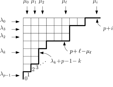
Figure 19. A pictorial explanation of why the choice (48) is a permutation of $(0,\cdots,p+i)$.

Let us now recall Lemma A.42. of [12] (see [12] for a proof).

Lemma 2.

Let $H^{+}$ and $E^{-}$ be $(p+i+1)\times(p+i+1)$ matrices which are inverse of each other. Let $(s_{0},s_{1},\cdots,s_{p-1},s_{0}^{\prime},s_{1}^{\prime},\cdots,s_{i}^{\prime})$ and $(t_{0},t_{1},\cdots,t_{p-1},t_{0}^{\prime},t_{1}^{\prime},\cdots,t_{i}^{\prime})$ be permutations of the sequence $(0,\cdots,p+i)$. Then

$$\det(H^{+}_{s_{m},t_{n}})_{0\leq m,n\leq p}=\epsilon\det(H^{+})\ \det(E^{-}_{t_{m}^{\prime},s_{n}^{\prime}})_{0\leq m,n\leq i}$$

where $\epsilon$ is the product of the signs of the two permutations.

We will use this lemma in the following particular case: let $\lambda_{0}\geq\lambda_{1}\geq\cdots\geq\lambda_{p-1}\geq 0$ be a partition of $\sum_{k=0}^{p-1}\lambda_{k}$ and $\mu_{0}\geq\mu_{1}\geq\cdots\geq\mu_{i}\geq 0$ the conjugate partition (with in particular $\sum_{k=0}^{p-1}\lambda_{k}=\sum_{k=0}^{i}\mu_{k}$). Then it is a classical result that $(s_{0},s_{1},\cdots,s_{p-1},s_{0}^{\prime},s_{1}^{\prime},\cdots,s_{i}^{\prime})$ with

(48) $$\begin{split}&s_{k}=\lambda_{k}+p-1-k,\quad k=0,\cdots,p-1\\ &s_{k}^{\prime}=p+k-\mu_{k},\quad k=0,\cdots,i\\ \end{split}$$

forms a permutation of the sequence $(0,\cdots,p+i)$. It simply corresponds to labelling each of the $p$ lines (resp. the $i+1$ columns) of the associated Young diagram by the index of its last vertical (resp. horizontal) segment, upon indexing this sequence of segments (which forms a broken line of length $p+i+1$) by $0,\cdots,p+i$ in the natural way (see Figure 19). For the other permutation $(t_{0},t_{1},\cdots,t_{p-1},t_{0}^{\prime},t_{1}^{\prime},\cdots,t_{i}^{\prime})$, we shall use

$$\begin{split}&t_{k}=p-1-k,\quad k=0,\cdots,p-1\\ &t_{k}^{\prime}=p+k,\quad k=0,\cdots,i\\ \end{split}$$

in which case $\epsilon=(-1)^{\sum_{k=0}^{p-1}\lambda_{k}}=(-1)^{\sum_{k=0}^{i}\mu_{k}}$ (the permutation $(t_{0},t_{1},\cdots,t_{p-1},t_{0}^{\prime},t_{1}^{\prime},\cdots,t_{i}^{\prime})$ corresponds indeed in Figure 19 to the case of a Young diagram without boxes, so that the broken line sticks to the left and upper sides. The permutation $(s_{0},s_{1},\cdots,s_{p-1},s_{0}^{\prime},s_{1}^{\prime},\cdots,s_{i}^{\prime})$ may be viewed as obtained from $(t_{0},t_{1},\cdots,t_{p-1},t_{0}^{\prime},t_{1}^{\prime},\cdots,t_{i}^{\prime})$ by successive additions of boxes to the Young diagram. Adding a box corresponds to performing a transposition so, each time a box is added, the sign of the permutation changes and $\epsilon$ is therefore nothing but $-1$ to the power the total number of boxes). In our case $\det(H^{+})=1$ and therefore

$$\det(E^{-}_{p+m,p+n-\mu_{n}})_{0\leq m,n\leq i}=(-1)^{\sum_{k=0}^{p-1}\lambda_{k}}\det(H^{+}_{\lambda_{m}+p-1-m,p-1-n})_{0\leq m,n\leq p}\ .$$

In other words, if we define, for $r\in\mathbb{Z}$, $L(r)$ as the line-vector of length $p$ whose $n$-th entry (for $n\in 0,\cdots,p-1$) is $h_{r+n+1}+c\,h_{r-n}-\sum_{q=1}^{n}(c^{2}-1)(-c)^{q-1}h_{r-n+q}$, and define, for any $(r_{0},\cdots,r_{p-1})\in\mathbb{Z}^{p}$, $M(r_{0},\cdots,r_{p-1})$ as the $p\times p$ matrix whose $m$-th row (for $m\in 0,\cdots,p-1$) is $L(r_{m})$, then the equality above rewrites as

$$\det(E^{-}_{p+m,p+n-\mu_{n}})_{0\leq m,n\leq i}=(-1)^{\sum_{k=0}^{p-1}\lambda_{k}}\det(M(r_{0},\cdots,r_{p-1})),$$

with $r_{m}=\lambda_{m}-m-1$. In particular, if we choose $\lambda_{k}=(i+1)$ for all $k=0,\cdots,p-1$, so that $\mu_{k}=p$ for all $k=0,\cdots,i$, we deduce

$$h_{i}^{(0)}=(BW)^{\frac{i(i+1)}{2}}(-1)^{p(i+1)}C_{p}^{i+1}\det(M(i,i-1,\cdots,i-p+1))$$

involving now the determinant of a matrix of fixed size $p\times p$, instead of a possibly arbitrarily large size $(i+1)\times(i+1)$.

To prove eq. (31), it remains to give an explicit form of this latter determinant in terms of the $x_{a}$’s and $c$. Let us define

$$\zeta_{a}(r)\equiv x_{a}^{r}-x_{a}^{-r}$$

for $a=1,\cdots p$ and any integer $r\geq 0$. Then, Lemma A.54. of [12] states that

Lemma 3.

$$\zeta_{a}(r)=\left(h_{r-p},h_{r-p+1}+h_{r-p-1},\cdots,h_{r-1}+h_{r-2p+1}\right)\cdot\bar{E}\cdot\left(\begin{matrix}\zeta_{a}(p)\\ \vdots\\ \zeta_{a}(1)\\ \end{matrix}\right)$$

with $h_{\ell}=h_{\ell}\left(x_{1},x_{2},\cdots,x_{p},\frac{1}{x_{1}},\frac{1}{x_{2}},\cdots,\frac{1}{x_{p}}\right)$ and $\bar{E}=(E_{m,n})_{0\leq m,n\leq p-1}$ the $p\times p$ matrix with matrix elements $E_{m,n}$ as in eq. (46).

A direct consequence of this lemma is that, if we now define, for $r\geq 0$

$$\xi_{a}(r)\equiv c\,\zeta_{a}(r)+\zeta_{a}(r+1)\ ,$$

we have

$$\begin{split}&\xi_{a}(r)=\left(\eta_{r-p},\eta_{r-p+1}+\eta_{r-p-1},\cdots,\eta_{r-1}+\eta_{r-2p+1}\right)\cdot\bar{E}\cdot\left(\begin{matrix}\zeta_{a}(p)\\ \vdots\\ \zeta_{a}(1)\\ \end{matrix}\right)\\ &\hbox{where}\ \eta_{r}=c\,h_{r}+h_{r+1}\ .\\ \end{split}$$

In other words, if we define for $r\in\mathbb{Z}$, $\widehat{L}(r)$ as the line-vector $(\eta_{r},\eta_{r+1}+\eta_{r-1},\cdots,\eta_{r+p-1}+\eta_{r-p+1})$, then for any $r\geq-p$,

$$\xi_{a}(p+r)=\widehat{L}(r)\cdot\overline{E}\cdot\left(\begin{matrix}\zeta_{a}(p)\\ \vdots\\ \zeta_{a}(1)\\ \end{matrix}\right)\ .$$

Hence, if we define, for any integers $r_{0},\cdots,r_{p-1}$, $\widehat{M}(r_{0},\cdots,r_{p-1})$ as the $p\times p$ matrix whose $m$-th row is $\widehat{L}(r_{m})$, then, since $\det(\bar{E})=1$, we have (for $r_{0},\cdots,r_{p-1}$ all at least $-p$)

$$\det(\widehat{M}(r_{0},\cdots,r_{p-1}))=\frac{\det\limits_{1\leq a^{\prime},a\leq p}\xi_{a}(p+r_{a^{\prime}-1})}{\det\limits_{1\leq a^{\prime},a\leq p}\zeta_{a}(p+1-a^{\prime})}$$

Figure 20. A pictorial representation of the successive (from left to right) actions of $\tau_{1},\tau_{2},\cdots$ on $L(r)$. The $(n+1)$-th column represents the set of indices $\ell$ of the various $h_{\ell}$ entering the linear combination of the $n$-th entry of $L(r),\tau_{1}L(r),\tau_{2}\circ\tau_{1}L(r),\cdots$ (from left to right). Each appearing index is represented by a dot at the corresponding height level beside which we indicate the corresponding coefficient. Here, we use the short hand notation $\kappa=1-c^{2}$. For instance, we indicated the entry of the $4$th column (corresponding to $n=3$) before and after subtractions (note that the $n$-th entry does not change after the $n$-th subtraction).

Now, looking at Figure 20, we have for any $r\in\mathbb{Z}$

$$L(r)=\tau_{p-1}\circ\tau_{p-2}\circ\cdots\circ\tau_{1}(\widehat{L}(r)),$$

where for $n\in 1,\cdots,p-1$, $\tau_{n}$ is the operator (on $p$-line-vectors) that subtracts $c$ times the $(n-1)$-th entry from the $n$-th entry. Hence,

$$M(r_{0},\cdots,r_{p-1})=\tau_{p-1}\circ\tau_{p-2}\circ\cdots\circ\tau_{1}(\widehat{M}(r_{0},\cdots,r_{p-1})),$$

where $\tau_{n}$ is now the operator on $p\times p$ matrices that subtracts $c$ times the $(n-1)$-th column from the $n$-th column. Since these column operations do not change the determinant, we have

$$\det(M(r_{0},\cdots,r_{p-1}))=\det(\widehat{M}(r_{0},\cdots,r_{p-1}))$$

and in particular,

$$\begin{split}\det(M(i,i-1,\cdots,i-p+1))&=\frac{\det\limits_{1\leq a^{\prime},a\leq p}\xi_{a}(i+(p+1-a^{\prime}))}{\det\limits_{1\leq a^{\prime},a\leq p}\zeta_{a}(p+1-a^{\prime})}\\ &=\frac{\det\limits_{1\leq a^{\prime},a\leq p}\xi_{a}(i+a^{\prime})}{\det\limits_{1\leq a^{\prime},a\leq p}\zeta_{a}(a^{\prime})}\\ &=\frac{\det\limits_{1\leq a^{\prime},a\leq p}((x_{a}+c)x_{a}^{i+a^{\prime}}-(1/x_{a}+c)x_{a}^{-(i+a^{\prime})})}{\det\limits_{1\leq a^{\prime},a\leq p}(x_{a}^{a^{\prime}}-x_{a}^{-a^{\prime}})})\\ &=\prod_{a=1}^{p}(1+c\,x_{a})\frac{\det\limits_{1\leq a^{\prime},a\leq p}(\gamma_{a}x_{a}^{i+a^{\prime}}-x_{a}^{-(i+1+a^{\prime})})}{\det\limits_{1\leq a^{\prime},a\leq p}(x_{a}^{a^{\prime}}-x_{a}^{-a^{\prime}})})\\ &\qquad\hbox{where}\ \gamma_{a}=\frac{c+x_{a}}{1+cx_{a}}\\ \end{split}$$

from which (up to simple transposition) eq. (31) follows.

Appendix C Generating functions for hard dimers

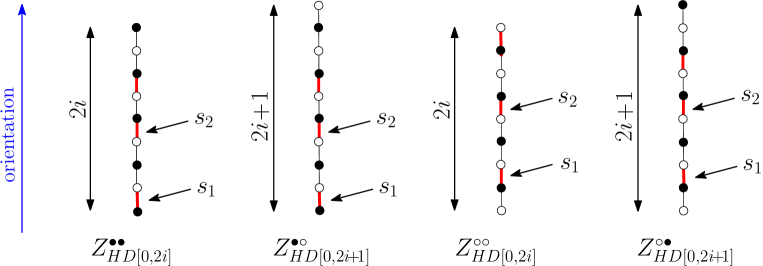
Figure 21. Example of configurations of hard dimers contributing to $Z_{HD[0,2i]}^{\bullet\bullet}$, $Z_{HD[0,2i+1]}^{\bullet\circ}$, $Z_{HD[0,2i]}^{\circ\circ}$ and $Z_{HD[0,2i+1]}^{\circ\bullet}$ respectively. The bicolored segments are viewed as oriented from bottom to top. A weight $s_{1}$ is assigned to each dimer (in red) lying on a link oriented (from bottom to top) from a black to a white node and a weight $s_{2}$ is assigned to each dimer lying on a link oriented from a white to a black node.

In this section, we shall derive a number of generating functions for hard dimers on bicolored segments. We denote by $Z_{HD[0,2i]}^{\bullet\bullet}\equiv Z_{HD[0,2i]}^{\bullet\bullet}(s_{1},s_{2})$ the generating function of hard dimers on an oriented segment (a finite oriented linear graph) made of $2i$ links whose nodes are bicolored alternatively in black and white and whose first and last node are black. Each link of the segment may be occupied by a dimer or not, with the constraint that a node is incident to at most one dimer. A weight $s_{1}$ is assigned to each dimer lying on a link oriented from a black to a white node and a weight $s_{2}$ is assigned to each dimer lying on a link oriented from a white to a black node, see Figure 21. We also introduce the generating functions $Z_{HD[0,2i]}^{\circ\circ}$, $Z_{HD[0,2i+1]}^{\bullet\circ}$ and $Z_{HD[0,2i+1]}^{\circ\bullet}$ with obvious definitions.

We introduce the parametrization

$$s_{1}=-\frac{x}{(c+x)(1+c\,x)}\qquad s_{2}=-\frac{c^{2}x}{(c+x)(1+c\,x)}\ .$$

It is achieved by taking for instance

$$c=\sqrt{\frac{s_{2}}{s_{1}}}\qquad x+\frac{1}{x}=-\frac{1+s_{1}+s_{2}}{c\,s_{1}}\ .$$

Note that exchanging $s_{1}$ and $s_{2}$ simply amounts to change $c$ into $1/c$, keeping $x$ unchanged. Note also that $x$ is only defined up to $x\leftrightarrow 1/x$ and that, for $(c,x)$ defined as above, our parametrization for $s_{1}$ and $s_{2}$ would have been realized as well by choosing $(-c,-x)$ instead. The reader is invited to verify that all the final formulas below for our hard dimer generating functions are in practice invariant under $x\leftrightarrow 1/x$ and under $(c,x)\leftrightarrow(-c,-x)$.

Upon decomposing the generating function according to the nature (i.e., occupied by a dimer or not) of the last link, we may write

$$\begin{split}&Z_{HD[0,2i]}^{\bullet\bullet}=Z_{HD[0,2i-1]}^{\bullet\circ}+s_{2}\,Z_{HD[0,2i-2]}^{\bullet\bullet}\\ &Z_{HD[0,2i+1]}^{\bullet\circ}=Z_{HD[0,2i]}^{\bullet\bullet}+s_{1}\,Z_{HD[0,2i-1]}^{\bullet\circ}\\ \end{split}$$

From the first equation for $i$ and $i+1$, we get

(49) $$\begin{split}&Z_{HD[0,2i-1]}^{\bullet\circ}=Z_{HD[0,2i]}^{\bullet\bullet}-s_{2}\,Z_{HD[0,2i-2]}^{\bullet\bullet}\\ &Z_{HD[0,2i+1]}^{\bullet\circ}=Z_{HD[0,2i+2]}^{\bullet\bullet}-s_{2}\,Z_{HD[0,2i]}^{\bullet\bullet}\\ \end{split}$$

and plugging these values in the second equation yields

$$Z_{HD[0,2i+2]}^{\bullet\bullet}=(1+s_{1}+s_{2})Z_{HD[0,2i]}^{\bullet\bullet}-s_{1}\,s_{2}\,Z_{HD[0,2i-2]}^{\bullet\bullet}$$

for all $i\geq 0$, with initial conditions $Z_{HD[0,0]}^{\bullet\bullet}=1$ and $Z_{HD[0,-2]}^{\bullet\bullet}=0$ (which implies $Z_{HD[0,2]}^{\bullet\bullet}=(1+s_{1}+s_{2})$ as wanted). Setting

$$\tau_{i}=(-c\,s_{1})^{-i}Z_{HD[0,2i]}^{\bullet\bullet}$$

and using the above parametrization of $s_{1}$ and $s_{2}$ (note in particular that $(-c\,s_{1})^{2}=s_{1}s_{2}$), the equation reads

$$\tau_{i+1}=\left(x+\frac{1}{x}\right)\tau_{i}-\tau_{i-1}$$

for $i\geq 0$ with $\tau_{0}=1$ and $\tau_{-1}=0$. Its solution is well known to be

$$\tau_{i}=\frac{x^{i+1}-x^{-(i+1)}}{x-x^{-1}}$$

which gives eventually

$$Z_{HD[0,2i]}^{\bullet\bullet}=\left(\frac{c}{(c+x)(1+c\,x)}\right)^{i}\frac{1-x^{2i+2}}{1-x^{2}}\ .$$

As for $Z_{HD[0,2i+1]}^{\bullet\circ}$, it is obtained from the second line of eq. (LABEL:eq:oddcase) which after simplification gives

$$Z_{HD[0,2i+1]}^{\bullet\circ}=(1+c\,x)\left(\frac{c}{(c+x)(1+c\,x)}\right)^{i+1}\frac{1-\frac{c+x}{1+c\,x}x^{2i+3}}{1-x^{2}}\ .$$

Finally, $Z_{HD[0,2i]}^{\circ\circ}$ and $Z_{HD[0,2i+1]}^{\circ\bullet}$ are obtained by changing $c$ into $1/c$, namely

$$\begin{split}&Z_{HD[0,2i]}^{\circ\circ}=\left(\frac{c}{(c+x)(1+c\,x)}\right)^{i}\frac{1-x^{2i+2}}{1-x^{2}}\\ &Z_{HD[0,2i+1]}^{\circ\bullet}=\left(1+\frac{x}{c}\right)\left(\frac{c}{(c+x)(1+c\,x)}\right)^{i+1}\frac{1-\frac{1+c\,x}{c+x}x^{2i+3}}{1-x^{2}}\ .\end{split}$$

Note that the fact that $Z_{HD[0,2i]}^{\bullet\bullet}=Z_{HD[0,2i]}^{\circ\circ}$ is obvious by reversing the orientation of the segment and exchanging the colors. For $c=1$ ($s_{1}=s_{2}$) all above formulas match well-known expressions for dimer generating functions on uncolored segments.

References

- [1] M. Albenque and J. Bouttier. Constellations and multicontinued fractions: application to eulerian triangulations. Discrete Math. Theor. Comput. Sci. Proc., pages 805–816, 2012. 24th International Conference on Formal Power Series and Algebraic Combinatorics (FPSAC 2012).
- [2] J. Ambjørn and T.G. Budd. Trees and spatial topology change in causal dynamical triangulations. J. Phys. A: Math. Theor., 46(31):315201, 2013.
- [3] J. Bouttier, P. Di Francesco, and E. Guitter. Geodesic distance in planar graphs. Nucl. Phys. B, 663(3):535–567, 2003.
- [4] J. Bouttier, P. Di Francesco, and E. Guitter. Statistics of planar graphs viewed from a vertex: a study via labeled trees. Nuclear Physics B, 675(3):631–660, 2003.
- [5] J. Bouttier, P. Di Francesco, and E. Guitter. Planar maps as labeled mobiles. Electron. J. Combin., 11(1):R69, 2004.
- [6] J. Bouttier, É. Fusy, and E. Guitter. On the two-point function of general planar maps and hypermaps, 2013. arXiv:1312.0502 [math.CO].
- [7] J. Bouttier and E. Guitter. Distance statistics in quadrangulations with no multiple edges and the geometry of minbus. Journal of Physics A: Mathematical and Theoretical, 43(20):205207, 2010.
- [8] J. Bouttier and E. Guitter. Planar maps and continued fractions. Comm. Math. Phys., 309(3):623–662, 2012.
- [9] J. Bouttier and E. Guitter. On irreducible maps and slices. Combinatorics, Probability and Computing, 23:914–972, 2014.
- [10] G. Chapuy, M. Marcus, and G. Schaeffer. A bijection for rooted maps on orientable surfaces. SIAM J. Discrete Math., 23(3):1587–1611, 2009.
- [11] R. Cori and B. Vauquelin. Planar maps are well labeled trees. Canad. J. Math., 33(5):1023–1042, 1981.
- [12] W. Fulton and J. Harris. Representation Theory: A First Course. Graduate Texts in Mathematics / Readings in Mathematics. Springer New York, 1991.
- [13] I.M. Gessel and X.G. Viennot. Binomial determinants, paths and hook length formulae. Adv. in Math., 58:300–321, 1985.
- [14] I.M. Gessel and X.G. Viennot. Determinants, paths, and plane partitions. preprint, 1989. available at http://people.brandeis.edu/ gessel/.
- [15] B. Jacquard and G. Schaeffer. A bijective census of nonseparable planar maps. J. Combin. Theory Ser. A, 83(1):1–20, 1998.
- [16] G. Schaeffer. Bijective census and random generation of Eulerian planar maps with prescribed vertex degrees. Electron. J. Combin., 4(1):R20, 1997.
- [17] G. Schaeffer. Conjugaison d’arbres et cartes combinatoires aléatoires. PhD thesis, Université Bordeaux I, 1998.