Influence Functions for Machine Learning: Nonparametric
Estimators for Entropies, Divergences and Mutual Informations

Abstract

We propose and analyze estimators for statistical functionals of one or more distributions under nonparametric assumptions. Our estimators are based on the theory of influence functions, which appear in the semiparametric statistics literature. We show that estimators based either on data-splitting or a leave-one-out technique enjoy fast rates of convergence and other favorable theoretical properties. We apply this framework to derive estimators for several popular information theoretic quantities, and via empirical evaluation, show the advantage of this approach over existing estimators.

1 Introduction

Entropies, divergences, and mutual informations are classical information-theoretic quantities that play fundamental roles in statistics, machine learning, and across the mathematical sciences. In addition to their use as analytical tools, they arise in a variety of applications including hypothesis testing, parameter estimation, feature selection, and optimal experimental design. In many of these applications, it is important to estimate these functionals from data so that they can be used in downstream algorithmic or scientific tasks. In this paper, we develop a recipe for estimating statistical functionals of one or more nonparametric distributions based on the notion of influence functions.

Entropy estimators are used in applications ranging from independent components analysis (Learned-Miller and John, 2003), intrinsic dimension estimation (Carter et al., 2010) and several signal processing applications (Hero et al., 2002). Divergence estimators are useful in statistical tasks such as two-sample testing. Recently they have also gained popularity as they are used to measure (dis)-similarity between objects that are modeled as distributions, in what is known as the “machine learning on distributions” framework (Dhillon et al., 2003; Póczos et al., 2011). Mutual information estimators have been used in in learning tree-structured Markov random fields (Liu et al., 2012), feature selection (Peng et al., 2005), clustering (Lewi et al., 2006) and neuron classification (Schneidman et al., 2002). In the parametric setting, conditional divergence and conditional mutual information estimators are used for conditional two sample testing or as building blocks for structure learning in graphical models. Nonparametric estimators for these quantities could potentially allow us to generalise several of these algorithms to the nonparametric domain. Our approach gives sample-efficient estimators for all these quantities (and many others), which often outperfom the existing estimators both theoretically and empirically.

Our approach to estimating these functionals is based on post-hoc correction of a preliminary estimator using the Von Mises Expansion van der Vaart (1998); Fernholz (1983). This idea has been used before in semiparametric statistics literature (Birgé and Massart, 1995; Robins et al., 2009). However, hitherto most studies are restricted to functionals of one distribution and have focused on a “data-split” approach which splits the samples for density estimation and functional estimation. While the data-split (DS) estimator is known to achieve the parametric convergence rate for sufficiently smooth densities Birgé and Massart (1995); Laurent (1996), in practical settings splitting the data results in poor empirical performance.

In this paper we introduce the calculus of influence functions to the machine learning community and considerably expand existing results by proposing a “leave-one-out” (LOO) estimator which makes efficient use of the data and has better empirical performance than the DS technique. We also extend the framework of influence functions to functionals of multiple distributions and develop both DS and LOO estimators. The main contributions of this paper are:

1. We propose a LOO technique to estimate functionals of a single distribution with the same convergence rates as the DS estimator. However, the LOO estimator performs better empirically.

2. We extend the framework to functionals of multiple distributions and analyse their convergence. Under sufficient smoothness both DS and LOO estimators achieve the parametric rate and the DS estimator has a limiting normal distribution.

3. We prove a lower bound for estimating functionals of multiple distributions. We use this to establish minimax optimality of the DS and LOO estimators under sufficient smoothness.

4. We use the approach to construct and implement estimators for various entropy, divergence, mutual information quantities and their conditional versions. A subset of these functionals are listed in Table 1. For several functionals, these are the only known estimators. Our software is publicly available at github.com/kirthevasank/if-estimators.

5. We compare our estimators against several other approaches in simulation. Despite the generality of our approach, our estimators are competitive with and in many cases superior to existing specialized approaches for specific functionals. We also demonstrate how our estimators can be used in machine learning applications via an image clustering task.

Our focus on information theoretic quantities is due to their relevance in machine learning applications, rather than a limitation of our approach. Indeed our techniques apply to any smooth functional.

History: We provide a brief history of the post-hoc correction technique and influence functions. We defer a detailed discussion of other approaches to estimating functionals to Section 5. To our knowledge, the first paper using a post-hoc correction estimator for was that of Bickel and Ritov (1988). The line of work following this paper analyzed integral functionals of a single one dimensional density of the form $\int\nu(p)$  (Bickel and Ritov, 1988; Birgé and Massart, 1995; Laurent, 1996; Kerkyacharian and Picard, 1996). A recent paper by Krishnamurthy et al. (2014) also extends this line to functionals of multiple densities, but only considers polynomial functionals of the form $\int p^{\alpha}q^{\beta}$ for densities $p$ and $q$. Moreover, all these works use data splitting. Our work builds on these by extending to a more general class of functionals and we propose the superior LOO estimator.

A fundamental quantity in the design of our estimators is the influence function, which appears both in robust and semiparametric statistics. Indeed, our work is inspired by that of Robins et al. (2009) and Emery et al. (1998) who propose a (data-split) influence-function based estimator for functionals of a single distribution. Their analysis for nonparametric problems rely on ideas from semiparametric statistics: they define influence functions for parametric models and then analyze estimators by looking at all parametric submodels through the true parameter.

2 Preliminaries

Let $\mathcal{X}$ be a compact metric space equipped with a measure $\mu$, e.g. the Lebesgue measure. Let $P$ and $Q$ be measures over $\mathcal{X}$ that are absolutely continuous w.r.t $\mu$. Let $p,q\in L_{2}(\mathcal{X})$ be the Radon-Nikodym derivatives with respect to $\mu$. We focus on estimating functionals of the form:

$$T(P) =T(p)=\phi\left(\int\nu(p)d\mu\right)\qquad\textrm{or}\qquad T(P,Q)=T(p,q)=\phi\left(\int\nu(p,q)d\mu\right),$$ (1)

where $\phi,\nu$ are real valued Lipschitz functions that twice differentiable. Our framework permits more general functionals – e.g. functionals based on the conditional densities – but we will focus on this form for ease of exposition. To facilitate presentation of the main definitions, it is easiest to work with functionals of one distribution $T(P)$. Define $\mathcal{M}$ to be the set of all measures that are absolutely continuous w.r.t $\mu$, whose Radon-Nikodym derivatives belong to $L_{2}(\mathcal{X})$.

Central to our development is the Von Mises expansion (VME), which is the distributional analog of the Taylor expansion. For this we introduce the Gâteaux derivative which imposes a notion of differentiability in topological spaces. We then introduce the influence function.

Definition 1.

The map $T^{\prime}:\mathcal{M}\rightarrow\mathbb{R}$ where $T^{\prime}(H;P)=\frac{\partial T(P+tH)}{\partial t}|_{t=0}$ is called the Gâteaux derivative at $P$ if the derivative exists and is linear and continuous in $H$. We say $T$ is Gâteaux differentiable at $P$ if $T^{\prime}$ exists at $P$.

Definition 2.

Let $T$ be Gâteaux differentiable at $P$. A function $\psi(\cdot;P):\mathcal{X}\rightarrow\mathbb{R}$ which satisfies $T^{\prime}(Q-P;P)=\int\psi(x;P)\mathrm{d}Q(x),$ is the influence function of $T$ w.r.t the distribution $P$.

The existence and uniqueness of the influence function is guaranteed by the Riesz representation theorem, since the domain of $T$ is a bijection of $L_{2}(\mathcal{X})$ and consequently a Hilbert space. The classical work of Fernholz (1983) defines the influence function in terms of the Gâteaux derivative by,

$$\psi(x,P)=T^{\prime}(\delta_{x}-P,P)=\frac{\partial T((1-t)P+t\delta_{x})}{\partial t}\Big{|}_{t=0},$$ (2)

where $\delta_{x}$ is the dirac delta function at $x$. While our functionals are defined only on non-atomic distributions, we can still use (2) to compute the influence function. The function computed this way can be shown to satisfy Definition 2.

Based on the above, the first order VME is,

$$T(Q)=T(P)+T^{\prime}(Q-P;P)+R_{2}(P,Q)=T(P)+\int\psi(x;P)\mathrm{d}Q(x)+R_{2}(P,Q),$$ (3)

where $R_{2}$ is the second order remainder. Gâteaux differentiability alone will not be sufficient for our purposes. In what follows, we will assign $Q\rightarrow F$ and $P\rightarrow\widehat{F}$, where $F$, $\widehat{F}$ are the true and estimated distributions. We would like to bound the remainder in terms of a distance between $F$ and $\widehat{F}$. By taking the domain of $T$ to be only measures with continuous densities, we can control $R_{2}$ using the $L_{2}$ metric of the densities. This essentially means that our functionals satisfy a stronger form of differentiability called Fréchet differentiability (van der Vaart, 1998; Fernholz, 1983) in the $L_{2}$ metric. Consequently, we can write all derivatives in terms of the densities, and the VME reduces to a functional Taylor expansion on the densities (Lemmas 9, 10 in Appendix A):

$$T(q) =T(p)+\phi^{\prime}\left(\int\nu(p)\right)\int(q-p)\nu^{\prime}(p)+R_{2}(p,q)$$

$$=T(p)+\int\psi(x;p)q(x)\mathrm{d}x+\mathcal{O}(\|p-q\|_{2}^{2}).$$ (4)

This expansion will be the basis for our estimators.

These ideas generalize to functionals of multiple distributions and to settings where the functional involves quantities other than the density. A functional $T(P,Q)$ of two distributions has two Gâteaux derivatives, $T^{\prime}_{i}(\cdot;P,Q)$ for $i=1,2$ formed by perturbing the $i$th argument with the other fixed. The influence functions $\psi_{1},\psi_{2}$ satisfy, $\forall P_{1},P_{2}\in\mathcal{M}$,

$$T_{1}^{\prime}(Q_{1}-P_{1};P_{1},P_{2})=\frac{\partial T(P_{1}+t(Q_{1}-P_{1}),P_{2})}{\partial t}\Big{|}_{t=0}=\int\psi_{1}(u;P_{1},P_{2})\mathrm{d}Q_{1}(u).$$ (5)

$$T_{2}^{\prime}(Q_{2}-P_{2};P_{1},P_{2})=\frac{\partial T(P_{1},P_{2}+t(Q_{2}-P_{2}))}{\partial t}\Big{|}_{t=0}=\int\psi_{2}(u;P_{1},P_{2})\mathrm{d}Q_{2}(u).$$

The VME can be written as,

$$T(q_{1},q_{2}) =T(p_{1},p_{2})+\int\psi_{1}(x;p_{1},p_{2})q_{1}(x)\mathrm{d}x+\int\psi_{2}(x;p_{1},p_{2})q_{2}(x)\mathrm{d}x$$

$$\hskip 14.45377pt+\mathcal{O}(\|p_{1}-q_{1}\|_{2}^{2})+\mathcal{O}(\|p_{2}-q_{2}\|_{2}^{2}).$$ (6)

3 Estimating Functionals

First consider estimating a functional of a single distribution, $T(f)=\phi(\int\nu(f)d\mu)$ from samples ${X_{1}^{n}}\sim f$. Using the VME (4), Emery et al. (1998) and Robins et al. (2009) suggested a natural estimator. If we use half of the data ${X_{1}^{n/2}}$ to construct a density estimate $\hat{f}^{(1)}=\hat{f}^{(1)}({X_{1}^{n/2}})$, then by (4):

$$T(f)-T(\hat{f}^{(1)})=\int\psi(x;\hat{f}^{(1)})f(x)d\mu+\mathcal{O}(\|f-\hat{f}^{(1)}\|_{2}^{2}).$$

Since the influence function does not depend on the unknown distribution $F$, the first term on the right hand side is simply an expectation of $\psi(X;\hat{f}^{(1)})$ at $F$. We use the second half of the data to estimate this expectation with its sample mean. This leads to the following preliminary estimator:

$${\widehat{T}^{(1)}_{\mathrm{\scriptscriptstyle DS}}}=T(\hat{f}^{(1)})+\frac{1}{n/2}\sum_{i=n/2+1}^{n}\psi(X_{i};\hat{f}^{(1)}).$$ (7)

We can similarly construct an estimator ${\widehat{T}^{(2)}_{\mathrm{\scriptscriptstyle DS}}}$ by using ${X_{n/2+1}^{n}}$ for density estimation and ${X_{1}^{n/2}}$ for averaging. Our final estimator is obtained via the average $\widehat{T}_{\mathrm{\scriptscriptstyle DS}}=({\widehat{T}^{(1)}_{\mathrm{\scriptscriptstyle DS}}}+{\widehat{T}^{(2)}_{\mathrm{\scriptscriptstyle DS}}})/2$. In what follows, we shall refer to this estimator as the Data-Split (DS) estimator.

The rate of convergence of this estimator is determined by the error in the VME $\mathcal{O}(\|f-\hat{f}^{(1)}\|_{2}^{2})$ and the $n^{-1/2}$ rate for estimating an expectation. Lower bounds from several literature (Laurent, 1996; Birgé and Massart, 1995) confirm minimax optimality of the DS estimator when $f$ is sufficiently smooth. The data splitting trick is commonly used in several other works Birgé and Massart (1995); Laurent (1996); Krishnamurthy et al. (2014). The analysis of DS estimators is straightforward as the rate directly follows from the Cauchy-Schwarz inequality. While in theory, DS estimators enjoy good rates of convergence, from a practical stand point, the data splitting is unsatisfying since using only half the data each for estimation and averaging invariably decreases the accuracy.

As an alternative, we propose a Leave-One-Out (LOO) version of the above estimator which makes more efficient use of the data,

$$\widehat{T}_{\mathrm{\scriptscriptstyle LOO}}=\frac{1}{n}\sum_{i=1}^{n}T(\hat{f}_{-i})+\psi(X_{i};\hat{f}_{-i}).$$ (8)

where $\hat{f}_{-i}$ is the kernel density estimate using all the samples ${X_{1}^{n}}$ except for $X_{i}$. Theoretically, we prove that the LOO Estimator achieves the same rate of convergence as the DS estimator but emprically it performs much better.

We can extend this method for functionals of two distributions. Akin to the one distribution case, we propose the following DS and LOO versions.

$${\widehat{T}^{(1)}_{\mathrm{\scriptscriptstyle DS}}} =T(\hat{f}^{(1)},\hat{g}^{(1)})+\frac{1}{n/2}\sum_{i=n/2+1}^{n}\psi_{f}(X_{i};\hat{f}^{(1)},\hat{g}^{(1)})+\frac{1}{m/2}\sum_{j=m/2+1}^{m}\psi_{g}(Y_{j};\hat{f}^{(1)},\hat{g}^{(1)}).$$ (9)

$$\widehat{T}_{\mathrm{\scriptscriptstyle LOO}} =\frac{1}{\max(n,m)}\sum_{i=1}^{\max(n,m)}T(\hat{f}_{-i},\hat{g}_{-i})+\psi_{f}(X_{i};\hat{f}_{-i},\hat{g}_{-i})+\psi_{g}(Y_{i};\hat{f}_{-i},\hat{g}_{-i}).$$ (10)

Here, $\hat{g}^{(1)},\hat{g}_{-i}$ are defined similar to $\hat{f}^{(1)},\hat{f}_{-i}$. For the DS estimator we swap the samples to compute ${\widehat{T}^{(2)}_{\mathrm{\scriptscriptstyle DS}}}$ and then average. For the LOO estimator, if $n>m$ we cycle through the points ${Y_{1}^{m}}$ until we have summed over all ${X_{1}^{n}}$ or vice versa. Note that $\widehat{T}_{\mathrm{\scriptscriptstyle LOO}}$ is asymmetric when $n\neq m$. A seemingly natural alternative would be to sum over all $nm$ pairings of $X_{i}$’s and $Y_{j}$’s. However, the latter approach is more computationally burdensome. Moreover, a straightforward modification of our analysis in Appendix D.2 shows that both estimators have the same rate of convergence if $n$ and $m$ are of the same order.

Examples: We demonstrate the generality of our framework by presenting estimators for several entropies, divergences and mutual informations and their conditional versions in Table 1. For several functionals in the table, these are the first estimators proposed. We hope that this table will serve as a good reference for practitioners. For several functionals (e.g. conditional and unconditional Rényi-$\alpha\;$divergence, conditional Tsallis-$\alpha\;$mutual information and more) the estimators are not listed only because the expressions are too long to fit into the table. Our software implements a total of $17$ functionals which include all the estimators in the table. In Appendix F we illustrate how to apply our framework to derive an estimator for any functional via an example.

As will be discussed in Section 5, when compared to other alternatives, our technique has several favourable properties. Computationally, the complexity of our method is $O(n^{2})$ when compared to $O(n^{3})$ for some other methods and for several functionals we do not require numeric integration. Additionally, unlike most other methods, we do not require any tuning of hyperparameters.

Functional	LOO Estimator
Tsallis-$\alpha\;$Entropy $\frac{1}{\alpha-1}\left(1-\int p^{\alpha}\right)$	$\frac{1}{1-\alpha}+\frac{1}{n}\sum_{i}\int\widehat{p}_{-i}^{\alpha}-\frac{\alpha}{\alpha-1}\widehat{p}_{-i}^{\alpha-1}(X_{i})$
Rényi-$\alpha\;$Entropy $\frac{-1}{\alpha-1}\log\int p^{\alpha}$	$\frac{\alpha}{\alpha-1}+\frac{1}{n}\sum_{i}\frac{-1}{\alpha-1}\log\int\widehat{p}_{-i}^{\alpha}-\widehat{p}_{-i}^{\alpha-1}(X_{i})+$
Shannon Entropy $-\int p\log p$	$-\frac{1}{n}\sum_{i}\log\widehat{p}_{-i}(X_{i})$
${L_{2}^{2}}$ Divergence $\int(p_{X}-p_{Y})^{2}$	$\frac{2}{n}\sum_{i}\widehat{p}_{X,-i}(X_{i})-\widehat{p}_{Y}(X_{i})-\int(\widehat{p}_{X,-i}-\widehat{p}_{Y})^{2}+\frac{2}{m}\sum_{j}\widehat{p}_{X}(Y_{j})-\widehat{p}_{Y,-j}(Y_{j})$
Hellinger Divergence $2-2\int{p_{X}}^{1/2}{p_{Y}}^{1/2}$	$2-\frac{1}{n}\sum_{i}\widehat{p}_{X,-i}^{-1/2}(X_{i})\widehat{p}_{Y}^{1/2}(X_{i})-\frac{1}{m}\sum_{j}\widehat{p}_{X}^{1/2}(Y_{j})\widehat{p}_{Y,-j}^{-1/2}(Y_{j})$
Chi-Squared Divergence $\int\frac{({p_{X}}-{p_{Y}})^{2}}{{p_{X}}}$	$-1+\frac{1}{n}\sum_{i}\frac{\widehat{p}_{Y}^{2}(X_{i})}{\widehat{p}_{X,-i}^{2}(X_{i})}+2\frac{1}{m}\sum_{j}\frac{\widehat{p}_{Y,-j}(Y_{j})}{\widehat{p}_{X}(Y_{j})}$
$f$-Divergence $\int\phi(\frac{{p_{X}}}{{p_{Y}}}){p_{Y}}$	$\frac{1}{n}\sum_{i}\phi^{\prime}\left(\frac{\widehat{p}_{X,-i}(X_{i})}{\widehat{p}_{Y}(X_{i})}\right)+\frac{1}{m}\sum_{j}\left(\phi\left(\frac{\widehat{p}_{Y,-j}(Y_{j})}{\widehat{p}_{X}(Y_{j})}\right)-\frac{\widehat{p}_{X}(Y_{j})}{\widehat{p}_{Y,-j}(Y_{j})}\phi\left(\frac{\widehat{p}_{X}(Y_{j})}{\widehat{p}_{Y,-j}(Y_{j})}\right)\right)$
Tsallis-$\alpha\;$Divergence $\frac{1}{\alpha-1}\left(\int{p_{X}}^{\alpha}{p_{Y}}^{1-\alpha}-1\right)$	$\frac{1}{1-\alpha}+\frac{\alpha}{\alpha-1}\frac{1}{n}\sum_{i}\left(\frac{\widehat{p}_{X,-i}(X_{i})}{\widehat{p}_{Y}(X_{i})}\right)^{\alpha-1}-\frac{1}{m}\sum_{j}\left(\frac{\widehat{p}_{X}(Y_{j})}{\widehat{p}_{Y,-j}(Y_{j})}\right)^{\alpha}$
KL divergence $\int p_{X}\log\frac{p_{X}}{p_{Y}}$	$1+\frac{1}{n}\sum_{i}\log\frac{\widehat{p}_{X,-i}(X_{i})}{\widehat{p}_{Y}(X_{i})}-\frac{1}{m}\sum_{j}\frac{\widehat{p}_{X}(Y_{j})}{\widehat{p}_{Y,-j}(Y_{j})}$
Conditional-Tsallis-$\alpha\;$divergence $\int p_{Z}\frac{1}{\alpha-1}\left(\int p_{X|Z}^{\alpha}p_{Y|Z}^{1-\alpha}-1\right)$	$\frac{1}{1-\alpha}+\frac{\alpha}{\alpha-1}\frac{1}{n}\sum_{i}\left(\frac{\widehat{p}_{XZ,-i}(V_{i})}{\widehat{p}_{YZ}(V_{i})}\right)^{\alpha-1}-\frac{1}{m}\sum_{j}\left(\frac{\widehat{p}_{XZ}(W_{j})}{\widehat{p}_{YZ,-j}(W_{j})}\right)^{\alpha}$
Conditional-KL divergence $\int p_{Z}\int p_{X|Z}\log\frac{p_{X|Z}}{p_{Y|Z}}$	$1+\frac{1}{n}\sum_{i}\log\frac{\widehat{p}_{XZ,-i}(V_{i})}{\widehat{p}_{YZ}(V_{i})}-\frac{1}{m}\sum_{j}\frac{\widehat{p}_{XZ}(W_{j})}{\widehat{p}_{YZ,-j}(W_{j})}$
Shannon Mutual Information $\int p_{XY}\log\frac{p_{XY}}{p_{X}p_{Y}}$	$\frac{1}{n}\sum_{i}\log\widehat{p}_{XY,-i}(X_{i},Y_{i})-\log\widehat{p}_{X,-i}(X_{i})-\log\widehat{p}_{Y,-i}(Y_{i})$
Conditional Tsallis-$\alpha\;$MI $\int p_{Z}\frac{1}{\alpha-1}\left(\int p_{X,Y|Z}^{\alpha}p_{X|Z}^{1-\alpha}p_{Y|Z}^{1-\alpha}-1\right)$	$\frac{1}{1-\alpha}+\frac{1}{\alpha-1}\frac{1}{n}\sum_{i}\alpha\left(\frac{\widehat{p}_{XYZ,-i}(X_{i},Y_{i},Z_{i})\widehat{p}_{Z}(Z_{i})}{\widehat{p}_{XZ,-i}(X_{i},Z_{i})\widehat{p}_{YZ,-i}(Y_{i},Z_{i})}\right)^{\alpha-1}$ $-(1-\alpha)\frac{1}{\alpha-1}\frac{1}{n}\sum_{i}\widehat{p}_{Z}^{\alpha-2}(Z_{i})\int\widehat{p}_{XYZ,-i}^{\alpha}(\cdot,\cdot,Z_{i})\widehat{p}_{XZ,-i}^{1-\alpha}(\cdot,Z_{i})$ $+\frac{1}{\alpha-1}\frac{1}{n}\sum_{i}(1-\alpha)\widehat{p}_{XZ,-i}^{-\alpha}(X_{i},Z_{i})\widehat{p}_{Z}^{1-\alpha}(Z_{i})\int\widehat{p}_{XYZ,-i}^{\alpha}(X_{i},\cdot,Z_{i})\widehat{p}_{YZ,-i}^{1-\alpha}(\cdot,Z_{i})$ $+\frac{1}{\alpha-1}\frac{1}{n}\sum_{i}(1-\alpha)\widehat{p}_{YZ,-i}^{-\alpha}(Y_{i},Z_{i})\widehat{p}_{Z}^{\alpha-1}(Z_{i})\int\widehat{p}_{XYZ,-i}^{\alpha}(\cdot,Y_{i},Z_{i})\widehat{p}_{XZ,-i}^{1-\alpha}(\cdot,\cdot)$

Table 1: Definitions of functionals and the corresponding estimators. Here $p_{X|Z},{p_{XZ}}$ etc. are conditional and joint distributions. For the conditional divergences we take $V_{i}=(X_{i},Z_{1i})$, $W_{j}=(Y_{j},Z_{2j})$ to be the samples from ${p_{XZ}},{p_{YZ}}$ respectively. For the mutual informations we have samples $(X_{i},Y_{i})\sim{p_{XY}}$ and for the conditional versions we have $(X_{i},Y_{i},Z_{i})\sim p_{XYZ}$.

4 Analysis

Some smoothness assumptions on the densities are warranted to make estimation tractable. We use the Hölder class, which is now standard in nonparametrics literature.

Definition 3 (Hölder Class).

Let $\mathcal{X}\subset\mathbb{R}^{d}$ be a compact space. For any $r=(r_{1},\dots,r_{d}),r_{i}\in\mathbb{N}$, define $|r|=\sum_{i}r_{i}$ and $D^{r}=\frac{\partial^{|r|}}{\partial x_{1}^{r_{1}}\dots\partial x_{d}^{r_{d}}}$. The Hölder class $\Sigma(s,L)$ is the set of functions on $L_{2}(\mathcal{X})$ satisfying,

$$|D^{r}f(x)-D^{r}f(y)|\leq L\|x-y\|^{s-r},\;\;$$

for all $r$ s.t. $|r|\leq\lfloor s\rfloor$ and for all $x,y\in\mathcal{X}$.

Moreover, define the Bounded Hölder Class $\Sigma(s,L,B^{\prime},B)$ to be $\left\{f\in\Sigma(s,L):B^{\prime}<f<B\right\}$. Note that large $s$ implies higher smoothness. Given $n$ samples ${X_{1}^{n}}$ from a $d$-dimensional density $f$, the kernel density estimator (KDE) with bandwidth $h$ is $\hat{f}(t)=1/(nh^{d})\sum_{i=1}^{n}K\left(\frac{t-X_{i}}{h}\right)$. Here $K:\mathbb{R}^{d}\rightarrow\mathbb{R}$ is a smoothing kernel Tsybakov (2008). When $f\in\Sigma(s,L)$, by selecting $h\in\Theta(n^{\frac{-1}{2s+d}})$ the KDE achieves the minimax rate of $\mathcal{O}_{P}(n^{\frac{-2s}{2s+d}})$ in mean squared error. Further, if $f$ is in the bounded Hölder class $\Sigma(s,L,B^{\prime},B)$ one can truncate the KDE from below at $B^{\prime}$ and from above at $B$ and achieve the same convergence rate (Birgé and Massart, 1995). In our analysis, the density estimators $\hat{f}^{(1)},\hat{f}_{-i},\hat{g}^{(1)},\hat{g}_{-i}$ are formed by either a KDE or a truncated KDE, and we will make use of these results.

We will also need the following regularity condition on the influence function. This is satisfied for smooth functionals including those in Table 1. We demonstrate this in our example in Appendix F.

Assumption 4.

For a functional $T(f)$, the influence function $\psi$ satisfies,

$$\mathbb{E}\big{[}(\psi(X;f^{\prime})-\psi(X;f))^{2}\big{]}\in\mathcal{O}(\|f-f^{\prime}\|^{2})\;\;\textrm{ as }\;\;\|f-f^{\prime}\|^{2}\rightarrow 0.$$

For a functional $T(f,g)$ of two distributions, the influence functions $\psi_{f},\psi_{g}$ satisfy,

$$\mathbb{E}_{f}\Big{[}(\psi_{f}(X;f^{\prime},g^{\prime})-\psi_{f}(X;f,g))^{2}\Big{]}\in\mathcal{O}(\|f-f^{\prime}\|^{2}+\|g-g^{\prime}\|^{2})\;\;\textrm{ as }\;\;\|f-f^{\prime}\|^{2},\|g-g^{\prime}\|^{2}\rightarrow 0.$$

$$\mathbb{E}_{g}\Big{[}(\psi_{g}(Y;f^{\prime},g^{\prime})-\psi_{g}(Y;f,g))^{2}\Big{]}\in\mathcal{O}(\|f-f^{\prime}\|^{2}+\|g-g^{\prime}\|^{2})\;\;\textrm{ as }\;\;\|f-f^{\prime}\|^{2},\|g-g^{\prime}\|^{2}\rightarrow 0.$$

Under the above assumptions, it is known Emery et al. (1998); Robins et al. (2009) that the DS estimator on a single distribution achieves the mean squared error (MSE) $\mathbb{E}[(\widehat{T}_{\mathrm{\scriptscriptstyle DS}}-T(f))^{2}]\in\mathcal{O}(n^{\frac{-4s}{2s+d}}+n^{-1})$ and further is asymptotically normal when $s>d/2$. We have reviewed them along with a proof in Appendix B. Note that Robins et al. (2009) analyse $\widehat{T}_{\mathrm{\scriptscriptstyle DS}}$ in the semiparametric setting. We present a simpler self contained analysis that directly uses the VME and has more interpretable assumptions. Bounding the bias and variance of the DS estimator to establish the convergence rate follows via a straightforward conditioning argument and Cauchy Schwarz. However, an attractive property is that the analysis is agnostic to the density estimator used provided it achieves the correct rates.

For the LOO estimator proposed in (8), we establish the following result.

Theorem 5 (Convergence of LOO Estimator for $T(f)$).

Let $f\in\Sigma(s,L,B,B^{\prime})$ and $\psi$ satisfy Assumption 4. Then, $\mathbb{E}[(\widehat{T}_{\mathrm{\scriptscriptstyle LOO}}-T(f))^{2}]$ is $\mathcal{O}(n^{\frac{-4s}{2s+d}})$ when $s<d/2$ and $\mathcal{O}(n^{-1})$ when $s\geq d/2$.

The key technical challenge in analysing the LOO estimator (when compared to the DS estimator) is in bounding the variance with several correlated terms in the summation. The bounded difference inequality is a popular trick used in such settings, but this requires a supremum on the influence functions which leads to significantly worse rates. Instead we use the Efron-Stein inequality which provides an integrated version of bounded differences that can recover the correct rate when coupled with Assumption 4. Our proof is contingent on the use of the KDE as the density estimator. While our empirical studies indicate that $\widehat{T}_{\mathrm{\scriptscriptstyle LOO}}$’s limiting distribution is normal (Fig 2), the proof seems challenging due to the correlation between terms in the summation. We conjecture that $\widehat{T}_{\mathrm{\scriptscriptstyle LOO}}$ is indeed asymptotically normal but for now leave it as an open problem.

We reiterate that while the convergence rates are the same for both DS and LOO estimators, the data splitting degrades empirical performance of $\widehat{T}_{\mathrm{\scriptscriptstyle DS}}$.

Now we turn our attention to functionals of two distributions. When analysing asymptotics we will assume that as $n,m\rightarrow\infty$, $n/(n+m)\rightarrow\zeta\in(0,1)$. Denote $N=n+m$. For the DS estimator (9) we generalise our analysis for one distribution to establish the theorem below.

Theorem 6 (Convergence/Asymptotic Normality of DS Estimator for $T(f,g)$).

Let $f,g\in\Sigma(s,L,B,B^{\prime})$ and $\psi_{f},\psi_{g}$ satisfy Assumption 4. Then, $\;\mathbb{E}[(\widehat{T}_{\mathrm{\scriptscriptstyle DS}}-T(f,g))^{2}]$ is $\mathcal{O}(n^{\frac{-4s}{2s+d}}+m^{\frac{-4s}{2s+d}})$ when $s<d/2$ and $\mathcal{O}(n^{-1}+m^{-1})$ when $s\geq d/2$. Further, when $s>d/2$ and when $\psi_{f},\psi_{g}\neq{\bf 0}$, $\widehat{T}_{\mathrm{\scriptscriptstyle DS}}$ is asymptotically normal,

$$\sqrt{N}(\widehat{T}_{\mathrm{\scriptscriptstyle DS}}-T(f,g))\xrightarrow[]{\mathcal{D}}\mathcal{N}\left(0,\frac{1}{\zeta}\mathbb{V}_{f}\left[\psi_{f}(X;f,g)\right]+\frac{1}{1-\zeta}\mathbb{V}_{g}\left[\psi_{g}(Y;f,g)\right]\right).$$ (11)

The asymptotic normality result is useful as it allows us to construct asymptotic confidence intervals for a functional. Even though the asymptotic variance of the influence function is not known, by Slutzky’s theorem any consistent estimate of the variance gives a valid asymptotic confidence interval. In fact, we can use an influence function based estimator for the asymptotic variance, since it is also a differentiable functional of the densities. We demonstrate this in our example in Appendix F.

The condition $\psi_{f},\psi_{g}\neq{\bf 0}$ is somewhat technical. When both $\psi_{f}$ and $\psi_{g}$ are zero, the first order terms vanishes and the estimator converges very fast (at rate $1/n^{2}$). However, the asymptotic behavior of the estimator is unclear. While this degeneracy occurs only on a meagre set, it does arise for important choices. One example is the null hypothesis $f=g$ in two-sample testing problems.

Finally, for the LOO estimator (10) on two distributions we have the following result.

Theorem 7 (Convergence of LOO Estimator for $T(f,g)$).

Let $f,g\in\Sigma(s,L,B,B^{\prime})$ and $\psi_{f},\psi_{g}$ satisfy Assumption 4. Then, $\;\mathbb{E}[(\widehat{T}_{\mathrm{\scriptscriptstyle LOO}}-T(f,g))^{2}]$ is $\mathcal{O}(n^{\frac{-4s}{2s+d}}+m^{\frac{-4s}{2s+d}})$ when $s<d/2$ and $\mathcal{O}(n^{-1}+m^{-1})$ when $s\geq d/2$.

For many functionals, a Hölderian assumption ($\Sigma(s,L)$) alone is sufficient to guarantee the rates in Theorems 5,6 and 7. However, for some functionals (such as the $\alpha$-divergences) we require $\hat{f},\hat{g},f,g$ to be bounded above and below. Existing results (Krishnamurthy et al., 2014; Birgé and Massart, 1995) demonstrate that estimating such quantities is difficult without this assumption.

Now we turn our attention to the question of statistical difficulty. Via lower bounds given by Birgé and Massart (1995) and Laurent (1996) we know that the DS and LOO estimators are minimax optimal when $s>d/2$ for functionals of one distribution. In the following theorem, we present a lower bound for estimating functionals of two distributions.

Theorem 8 (Lower Bound for $T(f,g)$).

Let $f,g\in\Sigma(s,L)$ and $\widehat{T}$ be any estimator for $T(f,g)$. Define $\tau=\min\{8s/(4s+d),1\}$. Then there exists a strictly positive constant $c$ such that,

$$\liminf_{n\rightarrow\infty}\;\inf_{\widehat{T}}\;\sup_{f,g\in\Sigma(s,L)}\mathbb{E}\big{[}(\widehat{T}-T(f,g))^{2}\big{]}\geq c\left(n^{-\tau}+m^{-\tau}\right).$$

Our proof, given in Appendix E, is based on LeCam’s method Tsybakov (2008) and generalises the analysis of Birgé and Massart (1995) for functionals of one distribution. This establishes minimax optimality of the DS/LOO estimators for functionals of two distributions when $s\geq d/2$. However, when $s<d/2$ there is a gap between our technique and the lower bound and it is natural to ask if it is possible to improve on our rates in this regime. A series of work (Birgé and Massart, 1995; Laurent, 1996; Kerkyacharian and Picard, 1996) shows that, for integral functionals of one distribution, one can achieve the $n^{-1}$ rate when $s>d/4$ by estimating the second order term in the functional Taylor expansion. This second order correction was also done for polynomial functionals of two distributions with similar statistical gains (Krishnamurthy et al., 2014). While we believe this is possible here, these estimators are conceptually complicated and computationally expensive – requiring $O(n^{3}+m^{3})$ effort when compared to the $O(n^{2}+m^{2})$ effort for our estimator. The first order estimator has a favorable balance between statistical and computational efficiency. Further, not much is known about the limiting distribution of second order estimators.

5 Comparison with Other Approaches

Estimation of statistical functionals under nonparametric assumptions has received considerable attention over the last few decades. A large body of work has focused on estimating the Shannon entropy– Beirlant et al. (1997) gives a nice review of results and techniques. More recent work in the single-distribution setting includes estimation of Rényi and Tsallis entropies (Leonenko and Seleznjev, 2010; Pál et al., 2010). There are also several papers extending some of these techniques to the divergence estimation (Krishnamurthy et al., 2014; Póczos and Schneider, 2011; Wang et al., 2009; Källberg and Seleznjev, 2012; Pérez-Cruz, 2008).

Many of the existing methods can be categorized as plug-in methods: they are based on estimating the densities either via a KDE or using $k$-Nearest Neighbors ($k$-NN) and evaluating the functional on these estimates. Plug-in methods are conceptually simple but unfortunately suffer several drawbacks. First, they typically have worse convergence rate than our approach, achieving the parametric rate only when $s\geq d$ as opposed to $s\geq d/2$ (Liu et al., 2012; Singh and Poczos, 2014). Secondly, using either the KDE or $k$-NN, obtaining the best rates for plug-in methods requires undersmoothing the density estimate and we are not aware for principled approaches for hyperparameter tuning here. In contrast, the bandwidth used in our estimators is the optimal bandwidth for density estimation, so a number of approaches such as cross validation are available. This is convenient for a practitioner as our method does not require tuning hyper parameters. Secondly, plugin methods based on the KDE always require computationally burdensome numeric integration. In our approach, numeric integration can be avoided for many functionals of interest (See Table 1).

There is also another line of work on estimating $f$-Divergences. Nguyen et al. (2010) estimate $f$-divergences by solving a convex program and analyse the technique when the likelihood ratio of the densities is in an RKHS. Comparing the theoretical results is not straightforward since it is not clear how to port their assumptions to our setting. Further, the size of the convex program increases with the sample size which is problematic for large samples. Moon and Hero (2014) use a weighted ensemble estimator for $f$-divergences. They establish asymptotically normality and the parametric convergence rates only when $s\geq d$, which is a stronger smoothness assumption than is required by our technique. Both these works only consider $f$-divergences. Our method has wider applicability and includes $f$-divergences as a special case.

6 Experiments

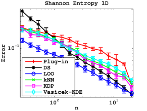
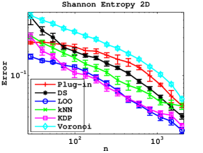
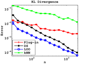
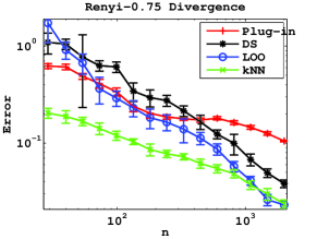
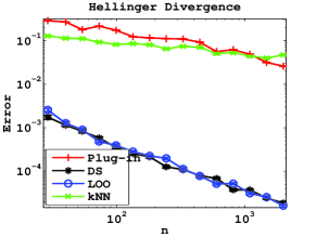
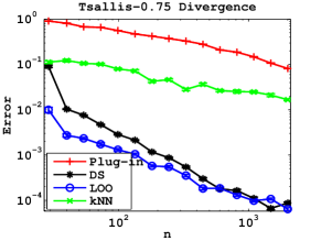
Figure 1: Comparison of DS/LOO estimators against alternatives on different functionals. The $y$-axis is the error $|\widehat{T}-T(f,g)|$ and the $x$-axis is the number of samples. All curves were produced by averaging over $50$ experiments. Some curves are slightly wiggly probably due to discretisation in hyperparameter selection.

6.1 Simulations

First, we compare the estimators derived using our methods on a series of synthetic examples in $1-4$ dimensions. For the DS/LOO estimators, we estimate the density via a KDE with the smoothing kernels constructed using Legendre polynomials (Tsybakov, 2008). In both cases and for the plug in estimator we choose the bandwidth by performing $5$-fold cross validation. The integration for the plug in estimator is approximated numerically.

We test the estimators on a series of synthetic datasets in $1-4$ dimension. The specifics of the data generating distributions and methods compared to are given below. The results are shown in Figures 1 and 2. We make the following observations. In most cases the LOO estimator performs best. The DS estimator approaches the LOO estimator when there are many samples but is generally inferior to the LOO estimator with few samples. This, as we have explained before is because data splitting does not make efficient use of the data. The $k$-NN estimator for divergences Póczos et al. (2011) requires choosing a $k$. For this estimator, we used the default setting for $k$ given in the software. As performance is sensitive to the choice of $k$, it performs well in some cases but poorly in other cases. We reiterate that our estimators do not require any setting of hyperparameters.

Next, we present some results on asymptotic normality. We test the DS and LOO estimators on a $4$-dimensional Hellinger divergence estimation problem. We use $4000$ samples for estimation. We repeat this experiment $200$ times and compare the empiritical asymptotic distribution (i.e. the $\sqrt{4000}(\widehat{T}-T(f,g))/\widehat{S}$ values where $\widehat{S}$ is the estimated asymptotic variance) to a $\mathcal{N}(0,1)$ distribution on a QQ plot. The results in Figure 2 suggest that both estimators are asymptotically normal.

Details: In our simulations, for the first figure comparing the Shannon Entropy in Fig 1 we generated data from the following one dimensional density,

$$f_{1}(t)=0.5+0.5t^{9}$$

For this, with probability $1/2$ we sample from the uniform distribution $U(0,1)$ on $(0,1)$ and otherwise sample $10$ points from $U(0,1)$ and pick the maximum. For the third figure in Fig 1 comparing the KL divergence, we generate data from the one dimensional density

$$f_{2}(t)=0.5+\frac{0.5t^{19}(1-t)^{19}}{B(20,20)}$$

where $B(\cdot,\cdot)$ is the Beta function. For this, with probability $1/2$ we sample from $U(0,1)$ and otherwise sample from a $\textrm{Beta}(20,20)$ distribution. The second and fourth figures of Fig 1 we sampled from a $2$ dimensional density where the first dimension was $f_{1}$ and the second was $U(0,1)$. The fifth and sixth were from a $2$ dimensional density where the first dimension was $f_{2}$ and the second was $U(0,1)$. In all figures of Fig. 2, the first distribution was a $4$-dimensional density where all dimensions are $f_{2}$. The latter was $U(0,1)^{4}$.

Methods compared to: In addition to the plug-in, DS and LOO estimators we perform comparisons with several other estimators. For the Shannon Entropy we compare our method to the $k$-NN estimator of Goria et al. (2005), the method of Stowell and Plumbley (2009) which uses $K-D$ partitioning, the method of Noughabi and Noughabi (2013) based on Vasicek’s spacing method and that of Learned-Miller and John (2003) based on Voronoi tessellation. For the KL divergence we compare against the $k$-NN method of Pérez-Cruz (2008) and that of Ramırez et al. (2009) based on the power spectral density representation using Szego’s theorem. For Rényi-$\alpha\;$, Tsallis-$\alpha\;$and Hellinger divergences we compared against the $k$-NN method of Póczos et al. (2011). Software for these estimators is obtained either directly from the papers or from Szabó (2014).

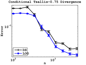
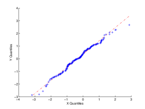
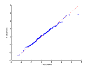
Figure 2: Fig 2: Comparison of the LOO vs DS estimator on estimating the Conditional Tsallis divergence in $4$ dimensions. Note that the plug-in estimator is intractable due to numerical integration. There are no other known estimators for the conditional tsallis divergence. Figs 2, 2: QQ plots obtained using $4000$ samples for Hellinger divergence estimation in $4$ dimensions using the DS and LOO estimators respectively.

6.2 Image Clustering Task

Here we demonstrate a simple image clustering task using a nonparametric divergence estimator. For this we use images from the ETH-80 dataset. The objective here is not to champion our approach for image clustering against all methods for image clustering out there. Rather, we just wish to demonstrate that our estimators can be easily and intuitively applied to many Machine Learning problems.

We use the three categories Apples, Cows and Cups and randomly select $50$ images from each category. Some sample images are shown in Fig 3. We convert the images to grey scale and extract the SIFT features from each image. The SIFT features are $128$-dimensional but we project it to $4$ dimensions via PCA. This is necessary because nonparametric methods work best in low dimensions. Now we can treat each image as a collection of features, and hence a sample from a $4$ dimensional distribution. We estimate the Hellinger divergence between these “distributions”. Then we construct an affinity matrix $A$ where the similarity metric between the $i$${}^{\textrm{th}}$ and $j$${}^{\textrm{th}}$ image is given by $A_{ij}=\exp(-\widehat{H}^{2}(X_{i},X_{j}))$. Here $X_{i}$ and $X_{j}$ denotes the projected SIFT samples from images $i$ and $j$ and $\widehat{H}(X_{i},X_{j})$ is the estimated Hellinger divergence between the distributions. Finally, we run a spectral clustering algorithm on the matrix $A$.

Figure 3 depicts the affinity matrix $A$ when the images were ordered according to their class label. The affinity matrix exhibits block-diagonal structure which indicates that our Hellinger divergence estimator can in fact identify patterns in the images. Our approach achieved a clustering accuracy of $92.47\%$. When we used the $k$-NN based estimator of Póczos et al. (2011) we achieved an accuracy of $90.04\%$. When we instead applied Spectral clustering naively, with $A_{ij}=\exp(-L_{2}(P_{i},P_{j})^{2})$ where $L_{2}(P_{i},P_{j})$ is the squared $L_{2}$ distance between the pixel intensities we achieved an accuracy of $70.18\%$. We also tried $A_{ij}=\exp(-\alpha\widehat{H}^{2}(X_{i},X_{j}))$ as the affinity for different choices of $\alpha$ and found that our estimator still performed best. We also experimented with the Rényi-$\alpha\;$and Tsallis-$\alpha\;$divergences and obtained similar results.

On the same note, one can imagine that these divergence estimators can also be used for a classification task. For instance we can treat $\exp(-\widehat{H}^{2}(X_{i},X_{j}))$ as a similarity metric between the images and use it in a classifier such as an SVM.

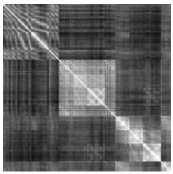
Figure 3: 3 Some sample images from the three categories apples, cows and cups. 3 The affinity matrix used in clustering.

7 Conclusion

We generalise existing results in Von Mises estimation by proposing an empirically superior LOO technique for estimating functionals and extending the framework to functionals of two distributions. We also prove a lower bound for the latter setting. We demonstrate the practical utility of our technique via comparisons against other alternatives and an image clustering application. An open problem arising out of our work is to derive the limiting distribution of the LOO estimator.

Appendix

Appendix A Auxiliary Results

Lemma 9 (VME and Functional Taylor Expansion).

Let $P,Q$ have densities $p,q$ and let $T(P)=\phi(\int\nu(p))$. Then the first order VME of $T(Q)$ around $P$ reduces to a functional Taylor expansion around $p$:

$$T(Q)=T(P)+T^{\prime}(Q-P;P)+R_{2}=T(p)+\phi^{\prime}\left(\int\nu(p)\right)\int\nu^{\prime}(p)(q-p)+R_{2}$$ (12)

Proof.

It is sufficient to show that the first order terms are equal.

$$T^{\prime}(Q-P;P) =\frac{\partial T((1-t)P+tQ)}{\partial t}\Big{|}_{t=0}=\frac{\partial}{\partial t}\phi\left(\int\nu((1-t)p+tq)\right)\big{|}_{t=0}$$

$$=\phi^{\prime}\left(\int\nu((1-t)p+tq)\right)\int\nu^{\prime}((1-t)p+tq)(q-p)\big{|}_{t=0}$$

$$=\phi^{\prime}\left(\int\nu(p)\right)\int\nu^{\prime}(p)(q-p)$$

∎

Lemma 10 (VME and Functional Taylor Expansion - Two Distributions).

Let $P_{1},P_{2},Q_{1},Q_{2}$ be distributions with densities $p_{1},p_{2},q_{1},q_{2}$. Let $T(P_{1},P_{2})=\int\nu(p_{1},p_{2})$. Then,

$$T(Q_{1},Q_{2}) =T(P_{1},P_{2})+T^{\prime}_{1}(Q_{1}-P_{1};P_{1},P_{2})+T_{2}^{\prime}(Q_{2}-P_{2};P_{1},P_{2})+R_{2}$$ (13)

$$=T(P_{1},P_{2})+\phi^{\prime}\left(\int\nu(p)\right)\Big{(}\int\frac{\partial\nu(p_{1}(x),p_{2}(x))}{\partial p_{1}(x)}(q_{1}-p_{1})\mathrm{d}x+$$

$$\hskip 43.36243pt\int\frac{\partial\nu(p_{1}(x),p_{2}(x))}{\partial p_{2}(x)}(q_{2}-p_{2})\mathrm{d}x\Big{)}+R_{2}$$

Proof.

Is similar to Lemma 9.
∎

Lemma 11.

Let $f,g$ be two densities bounded above and below on a compact space. Then for all $a,b$

$$\|f^{a}-g^{a}\|_{b}\in O(\|f-g\|_{b})$$

Proof.

Follows from the expansion,

$$\int|f^{a}-g^{a}|^{b}=\int|g^{a}(x)+a(f(x)-g(x))g_{*}^{a-1}(x)-g^{a}(x)|^{b}\leq a^{b}\sup|g_{*}^{b(a-1)}(x)|\int|f-g|^{b}.$$

Here $g_{*}(x)$ takes an intermediate value between $f(x)$ and $g(x)$. In the second step we have used the boundedness of $f$, $g$ to bound $f_{*}$. ∎

Finally, we will make use of the Efron Stein inequality stated below in our analysis.

Lemma 12 (Efron-Stein Inequality).

Let $X_{1},\dots,X_{n},X^{\prime}_{1},\dots,X^{\prime}_{n}$ be independent random variables where $X_{i},X^{\prime}_{i}\in\mathcal{X}_{i}$. Let $Z=f(X_{1},\dots,X_{n})$ and $Z^{(i)}=f(X_{1},\dots,X^{\prime}_{i},\dots,X_{n})$ where $f:\mathcal{X}_{1}\times\dots\times\mathcal{X}_{n}\rightarrow\mathbb{R}$. Then,

$$\mathbb{V}(Z)\;\leq\;\frac{1}{2}\;\mathbb{E}\left[\sum_{i=1}^{n}(Z-Z^{(i)})^{2}\right]$$

Appendix B Review: DS Estimator on a Single Distribution

This section is intended to be a review of the data split estimator used in Robins et al. (2009). The estimator was originally analysed in the semiparametric setting. However, in order to be self contained we provide an h analysis that directly uses the Von Mises Expansion. We state our main result below.

Theorem 13.

Suppose $f\in\Sigma(s,L,B,B^{\prime})$ and $\psi$ satisfies Assumption 4. Then, $\;\mathbb{E}[(\widehat{T}_{\mathrm{\scriptscriptstyle DS}}-T(f))^{2}]$ is $\mathcal{O}(n^{\frac{-4s}{2s+d}})$ when $s<d/2$ and $\mathcal{O}(n^{-1})$ when $s>d/2$. Further, when $s>d/2$ and when $\psi_{f},\psi_{g}\neq{\bf 0}$, $\widehat{T}_{\mathrm{\scriptscriptstyle DS}}$ is asymptotically normal.

$$\sqrt{n}(\widehat{T}_{\mathrm{\scriptscriptstyle DS}}-T(f,g))\xrightarrow[]{\mathcal{D}}\mathcal{N}\left(0,\frac{1}{\zeta}\mathbb{V}_{f}\left[\psi_{f}(X;f,g)\right]+\frac{1}{1-\zeta}\mathbb{V}_{g}\left[\psi_{g}(Y;f,g)\right]\right)$$ (14)

We begin the proof with a series of technical lemmas.

Lemma 14.

The Influence Function has zero mean. i.e. $\mathbb{E}_{P}[\psi(X;P)]=0$.

Proof.

$0=T^{\prime}(P-P;P)=\int\psi(x;P)\mathrm{d}P(x)$. ∎

Now we prove the following lemma on the preliminary estimator ${\widehat{T}^{(1)}_{\mathrm{\scriptscriptstyle DS}}}$.

Lemma 15 (Conditional Bias and Variance).

Let $\hat{f}^{(1)}$ be a consistent estimator for $f$ in the $L_{2}$ metric. Let $T$ have bounded second derivatives and let $\sup_{x}\psi(x;f)$ and $\mathbb{V}_{X\sim f}\psi(X;g)$ be bounded for all $g\in\mathcal{M}$. Then, the bias of the preliminary estimator ${\widehat{T}^{(1)}_{\mathrm{\scriptscriptstyle DS}}}$ (7) conditioned on ${X_{1}^{n/2}}$ is $\mathcal{O}(\|f-\hat{f}^{(1)}\|_{2}^{2})$. The conditional variance is $\mathcal{O}(1/n)$.

Proof.

First consider the conditional bias,

$$\mathbb{E}_{{X_{n/2+1}^{n}}}\left[{\widehat{T}^{(1)}_{\mathrm{\scriptscriptstyle DS}}}-T(f)|{X_{1}^{n/2}}\right] =\mathbb{E}_{{X_{n/2+1}^{n}}}\left[T(\hat{f}^{(1)})+\frac{2}{n}\sum_{i=n/2+1}^{n}\psi(X_{i};\hat{f}^{(1)})-T(f)|{X_{1}^{n/2}}\right]$$

$$=T(\hat{f}^{(1)})+\mathbb{E}_{f}\left[\psi(X;\hat{f}^{(1)})\right]-T(f)\in\mathcal{O}(\|\hat{f}^{(1)}-f\|_{2}^{2}).$$ (15)

The last step follows from the boundedness of the second derivative from which the first order functional Taylor expansion (4) holds. The conditional variance is,

$$\mathbb{V}_{X_{n/2+1}^{n}}\left[{\widehat{T}^{(1)}_{\mathrm{\scriptscriptstyle DS}}}|{X_{1}^{n/2}}\right]=\mathbb{V}_{X_{n/2+1}^{n}}\left[\frac{2}{n}\sum_{i=n/2+1}^{n}\psi(X;\hat{f}^{(1)})\Big{|}{X_{1}^{n/2}}\right]=\frac{2}{n}\mathbb{V}_{f}\left[\psi(X;\hat{f}^{(1)})\right]\in\mathcal{O}(n^{-1}).$$ (16)

∎

Lemma 16 (Asymptotic Normality).

Suppose in addition to the conditions in the lemma above we also have Assumption 4 and $\|\hat{f}^{(1)}-f\|_{2}\in o_{P}(n^{-1/4})$ and $\psi\neq{\bf 0}$. Then,

$$\sqrt{n}(\widehat{T}_{\mathrm{\scriptscriptstyle DS}}-T(f))\xrightarrow[]{\mathcal{D}}\mathcal{N}(0,\mathbb{V}_{f}\psi(X;f)).$$

Proof.

We begin with the following expansion around $\hat{f}^{(1)}$,

$$T(f) =T(\hat{f}^{(1)})+\int\psi(u;\hat{f}^{(1)})f(u)\mathrm{d}\mu(u)+O(\|\hat{f}^{(1)}-f\|^{2}).$$ (17)

First consider ${\widehat{T}^{(1)}_{\mathrm{\scriptscriptstyle DS}}}$. We can write

$$\sqrt{\frac{n}{2}}\left({\widehat{T}^{(1)}_{\mathrm{\scriptscriptstyle DS}}}-T(f)\right)=\sqrt{\frac{n}{2}}\left(T(\hat{f}^{(1)})+\frac{2}{n}\sum_{i=n/2+1}^{n}\psi(X_{i};\hat{f}^{(1)})-T(f)\right)$$ (18)

$$\hskip 21.68121pt=\sqrt{\frac{2}{n}}\sum_{i=n/2+1}^{n}\left[\psi(X_{i};\hat{f}^{(1)})-\psi(X_{i};f)-\left(\int\psi(u;\hat{f}^{(1)})f(u)\mathrm{d}u-\int\psi(u;f)f(u)\mathrm{d}u\right)\right]$$

$$\hskip 36.135pt+\sqrt{\frac{2}{n}}\sum_{i=n/2+1}^{n}\psi(X_{i};f)+\;\;\;\sqrt{n}\mathcal{O}\left(\|\hat{f}^{(1)}-f\|^{2}\right).$$

In the second step we used the VME in (17). In the third step, we added and subtracted $\sum_{i}\psi(X_{i};f)$ and also added $\mathbb{E}\psi(\cdot;f)=0$. Above, the third term is $o_{P}(1)$ as $\|\hat{f}^{(1)}-f\|_{2}\in o_{P}(n^{-1/4})$. The first term which we shall denote by $Q_{n}$ can also be shown to be $o_{P}(1)$ via Chebyshev’s inequality. It is sufficient to show $\mathbb{P}(|Q_{n}|>\epsilon|{X_{1}^{n/2}})\rightarrow 0$. First note that,

$$\mathbb{V}[Q_{n}|{X_{1}^{n/2}}] =\mathbb{V}\left[\sqrt{\frac{2}{n}}\sum_{i=n/2+1}^{n}\left(\psi(X_{i};\hat{f}^{(1)})-\psi(X_{i};f)-\left(\int\psi(u;\hat{f}^{(1)})f(u)\mathrm{d}u-\int\psi(u;f)f(u)\mathrm{d}u\right)\right)\Big{|}{X_{1}^{n/2}}\right]$$

$$=\mathbb{V}\left[\psi(X;\hat{f}^{(1)})-\psi(X;f)-\left(\int\psi(u;\hat{f}^{(1)})f(u)\mathrm{d}u-\int\psi(u;f)f(u)\mathrm{d}u\right)\Big{|}{X_{1}^{n/2}}\right]$$

$$\leq\mathbb{E}\left[\left(\psi(X;\hat{f}^{(1)})-\psi(X;f)\right)^{2}\right]\;\in\;\mathcal{O}(\|\hat{f}^{(1)}-f\|^{2})\rightarrow 0,$$ (19)

where the last step follows from Assumption 4. Now, $\mathbb{P}(|Q_{n}|>\epsilon|X_{1}^{n})\leq\mathbb{V}(Q_{n}|{X_{1}^{n/2}})/\epsilon\rightarrow 0$. Hence we have

$$\sqrt{\frac{n}{2}}({\widehat{T}^{(1)}_{\mathrm{\scriptscriptstyle DS}}}-T(f))=\sqrt{\frac{2}{n}}\sum_{i=n/2+1}^{n}\psi(X_{i};f)+o_{P}(1)$$

We can similarly show

$$\sqrt{\frac{n}{2}}({\widehat{T}^{(2)}_{\mathrm{\scriptscriptstyle DS}}}-T(f))=\sqrt{\frac{2}{n}}\sum_{i=n/2+1}^{n}\psi(X_{i};f)+o_{P}(1)$$

Therefore, by the CLT and Slutzky’s theorem,

$$\sqrt{n}(\widehat{T}_{\mathrm{\scriptscriptstyle DS}}-T(f)) =\frac{1}{\sqrt{2}}\left(\sqrt{\frac{n}{2}}({\widehat{T}^{(1)}_{\mathrm{\scriptscriptstyle DS}}}-T(f))+\sqrt{\frac{n}{2}}({\widehat{T}^{(2)}_{\mathrm{\scriptscriptstyle DS}}}-T(f))\right)$$

$$=n^{-1/2}\sum_{i=1}^{n}\psi(X_{i};f)+o_{P}(1)\;\;\xrightarrow[]{\mathcal{D}}\mathcal{N}(0,\mathbb{V}_{f}\psi(X;f)$$

∎

We are now ready to prove Theorem 13. Note that the brunt of the work for the DS estimator was in analysing the preliminary estimator $\widehat{T}_{\mathrm{\scriptscriptstyle DS}}$.

Proof of Theorem 13.

We first note that in a Hölder class, with $n$ samples the KDE achieves the rate $\mathbb{E}\|p-{\hat{p}}\|^{2}\in O(n^{\frac{-2s}{2s+d}})$. Then the bias of $\widehat{T}_{\mathrm{\scriptscriptstyle DS}}$ is,

$$\mathbb{E}_{{X_{1}^{n/2}}}\mathbb{E}_{{X_{n/2+1}^{n}}}\left[{\widehat{T}^{(1)}_{\mathrm{\scriptscriptstyle DS}}}-T(f)|{X_{1}^{n/2}}\right] =\mathbb{E}_{{X_{1}^{n/2}}}\left[O\left(\|f-\hat{f}^{(1)}\|^{2}\right)\right]\in O\left(n^{\frac{-2s}{2s+d}}\right)$$

It immediately follows that $\mathbb{E}\left[\widehat{T}_{\mathrm{\scriptscriptstyle DS}}-T(f)\right]\in O\left(n^{\frac{-2s}{2s+d}}\right)$. For the variance, we use Theorem 15 and the Law of total variance for ${\widehat{T}^{(1)}_{\mathrm{\scriptscriptstyle DS}}}$,

$$\mathbb{V}_{{X_{1}^{n}}}\left[{\widehat{T}^{(1)}_{\mathrm{\scriptscriptstyle DS}}}\right] =\frac{1}{n}\mathbb{E}_{{X_{1}^{n/2}}}\mathbb{V}_{f}\left[\psi(X;\hat{f}^{(1)},\hat{g})\right]++\mathbb{V}_{{X_{1}^{n/2}}}\left[\mathbb{E}_{{X_{n/2+1}^{n}}}\left[\widehat{T}_{\mathrm{\scriptscriptstyle DS}}-T(f)|{X_{1}^{n/2}}\right]\right]$$

$$\in O\left(\frac{1}{n}\right)+\mathbb{E}_{{X_{1}^{n/2}}}\left[O\left(\|f-\hat{f}^{(1)}\|^{4}\right)\right]$$

$$\in O\left(n^{-1}+n^{\frac{-4s}{2s+d}}\right)$$

In the second step we used the fact that $\mathbb{V}Z\leq\mathbb{E}Z^{2}$. Further, $\mathbb{E}_{{X_{1}^{n/2}}}\mathbb{V}_{f}\left[\psi(X;\hat{f}^{(1)})\right]$ is bounded since $\psi$ is bounded. The variance of $\widehat{T}_{\mathrm{\scriptscriptstyle DS}}$ can be bounded using the Cauchy Schwarz Inequality,

$$\mathbb{V}\left[\widehat{T}_{\mathrm{\scriptscriptstyle DS}}\right] =\mathbb{V}\left[\frac{{\widehat{T}^{(1)}_{\mathrm{\scriptscriptstyle DS}}}+{\widehat{T}^{(2)}_{\mathrm{\scriptscriptstyle DS}}}}{2}\right]=\frac{1}{4}\left(\mathbb{V}{\widehat{T}^{(1)}_{\mathrm{\scriptscriptstyle DS}}}+\mathbb{V}{\widehat{T}^{(2)}_{\mathrm{\scriptscriptstyle DS}}}+2\mathbb{C}\mathrm{ov}({\widehat{T}^{(1)}_{\mathrm{\scriptscriptstyle DS}}},{\widehat{T}^{(2)}_{\mathrm{\scriptscriptstyle DS}}})\right)$$

$$\leq\max\left(\mathbb{V}{\widehat{T}^{(1)}_{\mathrm{\scriptscriptstyle DS}}},\mathbb{V}{\widehat{T}^{(2)}_{\mathrm{\scriptscriptstyle DS}}}\right)\in O\left(n^{-1}+n^{\frac{-4s}{2s+d}}\right)$$

Finally for asymptotic normality, when $s>d/2$, $\mathbb{E}\|\hat{f}^{(1)}-f\|_{2}\in\mathcal{O}(n^{\frac{-s}{2s+d}})\in o\,(n^{-1/4})$. ∎

Appendix C Analysis of LOO Estimator

Proof of Theorem 5.

First note that we can bound the mean squared error via the bias and variance terms.

$$\mathbb{E}[(\widehat{T}_{\mathrm{\scriptscriptstyle LOO}}-T(f))^{2}]\leq|\mathbb{E}\widehat{T}_{\mathrm{\scriptscriptstyle LOO}}-T(f)|^{2}+\mathbb{E}[(\widehat{T}_{\mathrm{\scriptscriptstyle LOO}}-\mathbb{E}\widehat{T}_{\mathrm{\scriptscriptstyle LOO}})^{2}]$$

The bias is bounded via a straightforward conditioning argument.

$$\mathbb{E}|\widehat{T}_{\mathrm{\scriptscriptstyle LOO}}-T(f)| =\mathbb{E}[T(\hat{f}_{-i})+\psi(X_{i};\hat{f}_{-i})-T(f)]=\mathbb{E}_{X_{-i}}\left[\mathbb{E}_{X_{i}}[T(\hat{f}_{-i})+\psi(X_{i};\hat{f}_{-i})-T(f)]\right]$$

$$=\mathbb{E}_{X_{-i}}\left[\mathcal{O}(\|\hat{f}_{-i}-f\|^{2})\right]\;\leq C_{1}n^{\frac{-2s}{2s+d}}$$ (20)

for some constant $C_{1}$. The last step follows by observing that the KDE achieves the rate $n^{\frac{-2s}{2s+d}}$ in integrated squared error.

To bound the variance we use the Efron-Stein inequality. For this consider two sets of samples ${X_{1}^{n}}=\{X_{1},X_{2},\dots,X_{n}\}$ and ${X_{1}^{n}}^{\prime}=\{X^{\prime}_{1},X_{2},\dots,X_{n}\}$ which are the same except for the first point. Denote the estimators obtained using ${X_{1}^{n}}$ and ${X_{1}^{n}}^{\prime}$ by $\widehat{T}_{\mathrm{\scriptscriptstyle LOO}}$ and $\widehat{T}_{\mathrm{\scriptscriptstyle LOO}}^{\prime}$ respectively. To apply Efron-Stein we shall bound $\mathbb{E}[(\widehat{T}_{\mathrm{\scriptscriptstyle LOO}}-\widehat{T}_{\mathrm{\scriptscriptstyle LOO}}^{\prime})^{2}]$. Note that,

$$|\widehat{T}_{\mathrm{\scriptscriptstyle LOO}}-\widehat{T}_{\mathrm{\scriptscriptstyle LOO}}^{\prime}| \leq\frac{1}{n}|\psi(X_{1};\hat{f}_{-1})-\psi(X^{\prime}_{1};\hat{f}_{-1})|+\frac{1}{n}\sum_{i\neq 1}|T(\hat{f}_{-i})-T(\hat{f}_{-i}^{\prime})|$$

$$\hskip 43.36243pt+\frac{1}{n}\sum_{i\neq 1}|\psi(X_{i};\hat{f}_{-i})-\psi(X_{i};\hat{f}_{-i}^{\prime})|$$ (21)

The first term can be bounded by $2\|\psi\|_{\infty}/n$ using the boundedness of $\psi$. Each term inside the summation in the second term in (21) can be bounded via,

$$|T(\hat{f}_{-i})-T(\hat{f}_{-i}^{\prime})| \leq L_{\phi}\int|\nu(\hat{f}_{-i})-\nu(\hat{f}_{-i}^{\prime})|\leq L_{\nu}L_{\nu}\int|\hat{f}_{-i}-\hat{f}_{-i}^{\prime}|$$ (22)

$$\leq L_{\phi}L_{\nu}\int\frac{1}{nh^{d}}\Big{|}K\left(\frac{X_{1}-u}{h}\right)-K\left(\frac{X^{\prime}_{1}-u}{h}\right)\Big{|}\mathrm{d}u\leq\frac{\|K\|_{\infty}L_{\phi}L_{\nu}}{n}.$$

The substitution $(X_{1}-u)/h=z$ for integration eliminates the $1/h^{d}$. Here $L_{\phi},L_{\nu}$ are the Lipschitz constants of $\phi,\nu$. To apply Efron-Stein we need to bound the expectation of the LHS over $X_{1},X^{\prime}_{1},X_{2},\dots,X_{n}$. Since the first two terms in (21) are bounded pointwise by $\mathcal{O}(1/n^{2})$ they are also bounded in expectation. By Jensen’s inequality we can write,

$$|\widehat{T}_{\mathrm{\scriptscriptstyle LOO}}-\widehat{T}_{\mathrm{\scriptscriptstyle LOO}}^{\prime}|^{2} \leq\frac{12\|\psi\|^{2}_{\infty}}{n^{2}}+\frac{3\|K\|^{2}_{\infty}L^{2}_{\phi}L^{2}_{\nu}}{n^{2}}+\frac{3}{n^{2}}\left(\sum_{i\neq 1}|\psi(X_{i};\hat{f}_{-i})-\psi(X_{i};\hat{f}_{-i}^{\prime})|\right)^{2}$$ (23)

For the third, such a pointwise bound does not hold so we will directly bound the expectation.

$$\sum_{1\neq i,j}\mathbb{E}\Big{[}|\psi(X_{i};\hat{f}_{-i})-\psi(X_{i};\hat{f}_{-i}^{\prime})||\psi(X_{j};\hat{f}_{-j})-\psi(X_{j};\hat{f}_{-j}^{\prime})|\Big{]}$$ (24)

We then have,

$$\mathbb{E}\big{[}(\psi(X_{i};\hat{f}_{-i})-\psi(X_{i};\hat{f}_{-i}^{\prime}))^{2}\big{]} \leq\mathbb{E}_{X_{1},X^{\prime}_{1}}\left[C\int|\hat{f}_{-i}-\hat{f}_{-i}^{\prime}|^{2}\right]$$

$$\leq CB^{2}\int\frac{1}{n^{2}h^{2d}}\left(K\left(\frac{x_{1}-u}{h}\right)-K\left(\frac{x^{\prime}_{1}-u}{h}\right)\right)^{2}\mathrm{d}x_{1}\mathrm{d}x^{\prime}_{1}u$$

$$\leq\frac{2CB^{2}\|K\|^{2}_{\infty}}{n^{2}}$$

I the first step we have used Assumption 4 and in the last step the substitutions $(x_{1}-x_{i})/h=u$ and $(x_{1}-x_{j})/h=v$ removes the $1/h^{d}$ twice. Then, by applying Cauchy Schwarz each term inside the summation in (24) is $\mathcal{O}(1/n^{2})$.

Since each term inside equation (24) is $\mathcal{O}(1/n^{2})$ and there are $(n-1)^{2}$ terms it is $\mathcal{O}(1)$. Combining all these results with equation (23) we get,

$$\mathbb{E}[(\widehat{T}_{\mathrm{\scriptscriptstyle LOO}}-\widehat{T}_{\mathrm{\scriptscriptstyle LOO}}^{\prime})^{2}]\in\mathcal{O}\left(\frac{1}{n^{2}}\right)$$

Now, by applying the Efron-Stein inequality we get $\mathbb{V}(\widehat{T}_{\mathrm{\scriptscriptstyle LOO}})\leq\frac{C}{2n}$. Therefore the mean squared error $\mathbb{E}[(T-\widehat{T}_{\mathrm{\scriptscriptstyle LOO}})^{2}]\in\mathcal{O}(n^{-\frac{4s}{2s+d}}+n^{-1})$ which completes the proof. ∎

Appendix D Proofs of Results on Functionals of Two Distributions

D.1 DS Estimator

We generalise the results in Appendix B to analyse the DS estimator for two distributions. As before we begin with a series of lemmas.

Lemma 17.

The influence functions have zero mean. I.e.

$$\mathbb{E}_{P_{1}}[\psi_{1}(X;P_{1};P_{2})]=0\hskip 7.22743pt\forall P_{2}\in\mathcal{M}\hskip 36.135pt\mathbb{E}_{P_{2}}[\psi_{2}(Y;P_{1};P_{2})]=0\hskip 7.22743pt\forall P_{1}\in\mathcal{M}$$ (25)

Proof.

$0=T^{\prime}_{i}(P_{i}-P_{i};P_{1};P_{2})=\int\psi_{i}(u;P_{1},P_{2})\mathrm{d}P_{i}(u)$ for $i=1,2$. ∎

Lemma 18 (Bias & Variance of (9)).

Let $\hat{f}^{(1)},\hat{g}^{(1)}$ be consistent estimators for $f,g$ in the $L_{2}$ sense. Let $T$ have bounded second derivatives and let $\sup_{x}\psi_{f}(x;f,g)$, $\sup_{x}\psi_{g}(x;f,g)$, $\mathbb{V}_{f}\psi(X;f^{\prime},g^{\prime})$, $\mathbb{V}_{g}\psi_{g}(X;f^{\prime},g^{\prime})$ be bounded for all $f,f^{\prime},g,g^{\prime}\in\mathcal{M}$. Then the bias of ${\widehat{T}^{(1)}_{\mathrm{\scriptscriptstyle DS}}}$ conditioned on ${X_{1}^{n/2}},{Y_{1}^{m/2}}$ is $|T-\mathbb{E}[{\widehat{T}^{(1)}_{\mathrm{\scriptscriptstyle DS}}}|{X_{1}^{n/2}},{Y_{1}^{m/2}}]\in\mathcal{O}(\|f-\hat{f}^{(1)}\|^{2}+\|g-\hat{g}^{(1)}\|^{2})$. The conditional variance is $\mathbb{V}[{\widehat{T}^{(1)}_{\mathrm{\scriptscriptstyle DS}}}|{X_{1}^{n/2}},{Y_{1}^{m/2}}]\in\mathcal{O}(n^{-1}+m^{-1})$.

Proof.

First consider the bias conditioned on ${X_{1}^{n/2}},{Y_{1}^{m/2}}$,

$$\mathbb{E}\left[{\widehat{T}^{(1)}_{\mathrm{\scriptscriptstyle DS}}}-T(f,g)|{X_{1}^{n/2}},{Y_{1}^{m/2}}\right]$$

$$\hskip 14.45377pt=\mathbb{E}\left[T(\hat{f}^{(1)},\hat{g}^{(1)})+\frac{2}{n}\sum_{i=n/2+1}^{n}\psi_{f}(X_{i};\hat{f}^{(1)},\hat{g}^{(1)})+\frac{2}{m}\sum_{j=m/2+1}^{m}\psi_{g}(Y_{j};\hat{f}^{(1)},\hat{g}^{(1)})-T(f,g)\Bigg{|}{X_{1}^{n/2}},{Y_{1}^{m/2}}\right]$$

$$\hskip 14.45377pt=T(\hat{f}^{(1)},\hat{g}^{(1)})+\int\psi_{f}(x;\hat{f}^{(1)},\hat{g}^{(1)})f(x)\mathrm{d}\mu(x)+\int\psi_{g}(x;\hat{f}^{(1)},\hat{g}^{(1)})g(x)\mathrm{d}\mu(x)-T(f,g)$$

$$\hskip 14.45377pt=\mathcal{O}\left(\|f-\hat{f}^{(1)}\|^{2}+\|g-\hat{g}^{(1)}\|^{2}\right)$$

The last step follows from the boundedness of the second derivatives from which the first order functional Taylor expansion (6) holds. The conditional variance is,

$$\mathbb{V}\left[{\widehat{T}^{(1)}_{\mathrm{\scriptscriptstyle DS}}}|{X_{1}^{n/2}},{Y_{1}^{m/2}}\right] =\mathbb{V}\left[\frac{1}{n}\sum_{i=n+1}^{2n}\psi_{f}(X_{i};\hat{f}^{(1)},\hat{g}^{(1)})\Big{|}{X_{1}^{n/2}}\right]+\mathbb{V}\left[\frac{1}{m}\sum_{j=m+1}^{2m}\psi_{g}(Y_{j};\hat{f}^{(1)},\hat{g}^{(1)})\Big{|}{Y_{1}^{m/2}}\right]$$

$$=\frac{1}{n}\mathbb{V}_{f}\left[\psi_{f}(X;\hat{f}^{(1)},\hat{g}^{(1)})\right]+\frac{1}{m}\mathbb{V}_{g}\left[\psi_{g}(Y;\hat{f}^{(1)},\hat{g}^{(1)})\right]\in\mathcal{O}\left(\frac{1}{n}+\frac{1}{m}\right)$$

The last step follows from the boundedness of the variance of the influence functions. ∎

The following lemma characterises conditions for asymptotic normality.

Lemma 19 (Asymptotic Normality).

Suppose, in addition to the conditions in Theorem 18 above and the regularity assumption 4 we also have $\|\hat{f}-f\|\in o_{P}(n^{-1/4}),\|\hat{g}-g\|\in o_{P}(m^{-1/4})$ and $\psi_{f},\psi_{g}\neq{\bf 0}$. Then we have asymptotic Normality for $\widehat{T}_{\mathrm{\scriptscriptstyle DS}}$,

$$\sqrt{N}(\widehat{T}_{\mathrm{\scriptscriptstyle DS}}-T(f,g))\xrightarrow[]{\mathcal{D}}\mathcal{N}\left(0,\frac{1}{\zeta}\mathbb{V}_{f}\left[\psi_{f}(X;f,g)\right]+\frac{1}{1-\zeta}\mathbb{V}_{g}\left[\psi_{g}(Y;f,g)\right]\right)$$ (26)

Proof.

We begin with the following expansions around $(\hat{f}^{(1)},\hat{g}^{(1)})$,

$$T(f,g)=T(\hat{f}^{(1)},\hat{g}^{(1)})+\int\psi_{f}(u;\hat{f}^{(1)},\hat{g}^{(1)})f(u)\mathrm{d}u+\int\psi_{g}(u;\hat{f}^{(1)},\hat{g}^{(1)})g(u)\mathrm{d}u\;+$$

$$\hskip 72.26999pt\mathcal{O}\left(\|f-\hat{f}^{(1)}\|^{2}+\|g-\hat{g}^{(1)}\|^{2}\right)$$

Consider ${\widehat{T}^{(1)}_{\mathrm{\scriptscriptstyle DS}}}$. We can write

$$\sqrt{\frac{N}{2}}({\widehat{T}^{(1)}_{\mathrm{\scriptscriptstyle DS}}}-T(f))$$ (27)

$$\hskip 21.68121pt=\sqrt{\frac{N}{2}}\left(T(\hat{f}^{(1)},\hat{g}^{(1)})+\frac{2}{n}\sum_{i=n/2+1}^{n}\psi_{f}(X_{i};f,g)+\frac{2}{m}\sum_{j=m/2+1}^{m}\psi_{g}(Y_{j};f,g)-T(f,g)\right)$$

$$\hskip 21.68121pt=\sqrt{\frac{N}{2}}\Bigg{(}\frac{2}{n}\sum_{i=n/2+1}^{n}\psi(X_{i};\hat{f}^{(1)},\hat{g}^{(1)})+\frac{2}{m}\sum_{j=m/2+1}^{m}\psi(X_{j};\hat{f}^{(1)},\hat{g}^{(1)})-\mathbb{E}_{f}\left[\psi(X;\hat{f}^{(1)},\hat{g}^{(1)})\right]$$

$$\hskip 43.36243pt-\mathbb{E}_{g}\left[\psi(X;\hat{f}^{(1)},\hat{g}^{(1)})\right]\Bigg{)}+\sqrt{N}O\left(\|f-\hat{f}^{(1)}\|^{2}+\|g-\hat{g}^{(1)}\|^{2}\right)$$

$$\hskip 21.68121pt=\sqrt{\frac{2N}{n}}n^{-1/2}\sum_{i=n/2+1}^{n}\left(\psi_{f}(X_{i};\hat{f}^{(1)},\hat{g}^{(1)})-\psi_{f}(X_{i};f,g)-(\mathbb{E}_{f}\psi_{f}(X;\hat{f}^{(1)},\hat{g}^{(1)})+\mathbb{E}_{f}\psi_{f}(X;f,g))\right)+$$

$$\hskip 28.90755pt\sqrt{\frac{2N}{m}}m^{-1/2}\sum_{j=m/2+1}^{m}\left(\psi_{g}(Y_{j};\hat{f}^{(1)},\hat{g}^{(1)})-\psi_{g}(Y_{j};f,g)-(\mathbb{E}_{g}\psi_{g}(Y;\hat{f}^{(1)},\hat{g}^{(1)})+\mathbb{E}_{g}\psi_{g}(Y;f,g))\right)+$$

$$\hskip 28.90755pt\sqrt{\frac{2N}{n}}n^{-1/2}\sum_{i=n/2+1}^{n}\psi_{f}(X_{i};f,g)\,+\,\sqrt{\frac{2N}{m}}m^{-1/2}\sum_{j=m/2+1}^{m}\psi_{g}(Y_{j};f,g)\,+\,$$

$$\hskip 43.36243pt\sqrt{N}\mathcal{O}\left(\|f-\hat{f}^{(1)}\|^{2}+\|g-\hat{g}^{(1)}\|^{2}\right)$$

The fifth term is $o_{P}(1)$ by the assumptions. The first and second terms are also $o_{P}(1)$ . To see this, denote the first term by $Q_{n}$.

$$\mathbb{V}\left[Q_{n}|{X_{1}^{n/2}},{Y_{1}^{m/2}}\right] =\frac{N}{n}\mathbb{V}_{f}\left[\sum_{i=n/2+1}^{n}\left(\psi_{f}(X;\hat{f}^{(1)},\hat{g}^{(1)})-\psi_{f}(X;f,g)-(\mathbb{E}_{f}\psi_{f}(X;\hat{f}^{(1)},\hat{g}^{(1)})+\mathbb{E}_{f}\psi_{f}(X;f,g))\right)\right]$$

$$\leq\frac{N}{n}\mathbb{E}_{f}\left[\left(\psi_{f}(X_{i};\hat{f}^{(1)},\hat{g}^{(1)})-\psi_{f}(X_{i};f,g)\right)^{2}\right]\rightarrow 0$$

where we have used the regularity assumption 4. Further, $\mathbb{P}(|Q_{n}|>\epsilon|{X_{1}^{n/2}},{Y_{1}^{m/2}})\leq\mathbb{V}[Q_{n}|{X_{1}^{n/2}},{Y_{1}^{m/2}}]\ \epsilon\rightarrow 0$, hence the first term is $o_{P}(1)$. The proof for the second term is similar. Therefore we have,

$$\sqrt{\frac{N}{2}}({\widehat{T}^{(1)}_{\mathrm{\scriptscriptstyle DS}}}-T(f))=\sqrt{\frac{2N}{n}}n^{-1/2}\sum_{i=n/2+1}^{n}\psi_{f}(X_{i};f,g)\,+\,\sqrt{\frac{2N}{m}}m^{-1/2}\sum_{j=m/2+1}^{m}\psi_{g}(Y_{j};f,g)\,+\,o_{P}(1)$$

Using a similar argument on ${\widehat{T}^{(2)}_{\mathrm{\scriptscriptstyle DS}}}$ we get,

$$\sqrt{\frac{N}{2}}({\widehat{T}^{(2)}_{\mathrm{\scriptscriptstyle DS}}}-T(f))=\sqrt{\frac{2N}{n}}n^{-1/2}\sum_{i=1}^{n/2}\psi_{f}(X_{i};f,g)\,+\,\sqrt{\frac{2N}{m}}m^{-1/2}\sum_{j=1}^{m/2}\psi_{g}(Y_{j};f,g)\,+\,o_{P}(1)$$

Therefore,

$$\sqrt{N}({\widehat{T}^{(2)}_{\mathrm{\scriptscriptstyle DS}}}-T(f)) =\sqrt{2}\left(\sqrt{\frac{2N}{n}}n^{-1/2}\sum_{i=1}^{n}\psi_{f}(X_{i};f,g)\,+\,\sqrt{\frac{2N}{m}}m^{-1/2}\sum_{j=1}^{m}\psi_{g}(Y_{j};f,g)\,\right)\,+\,o_{P}(1)$$

$$=\sqrt{\frac{N}{n}}n^{-1/2}\sum_{i=1}^{2n}\psi_{f}(X_{i};f,g)\,+\,\sqrt{\frac{N}{m}}m^{-1/2}\sum_{j=1}^{2m}\psi_{g}(Y_{j};f,g)\,+\,o_{P}(1)$$

By the CLT and Slutzky’s theorem this converges weakly to the RHS of (26). ∎

We are now ready to prove the rates of convergence for the DS estimator in the Hölder class.

Proof of Theorem 13.

. We first note that in a Hölder class, with $n$ samples the KDE achieves the rate $\mathbb{E}\|p-{\hat{p}}\|^{2}\in O(n^{\frac{-2s}{2s+d}})$. Then the bias for the preliminary estimator ${\widehat{T}^{(1)}_{\mathrm{\scriptscriptstyle DS}}}$ is,

$$\mathbb{E}\left[{\widehat{T}^{(1)}_{\mathrm{\scriptscriptstyle DS}}}-T(f,g)|{X_{1}^{n/2}},{Y_{1}^{m/2}}\right] =\mathbb{E}_{{X_{1}^{n/2}},{Y_{1}^{m/2}}}\left[O\left(\|f-\hat{f}^{(1)}\|^{2}+\|g-\hat{g}^{(1)}\|^{2}\right)\right]$$

$$\in O\left(n^{\frac{-2s}{2s+d}}+m^{\frac{-2s}{2s+d}}\right)$$

The same could be said about ${\widehat{T}^{(2)}_{\mathrm{\scriptscriptstyle DS}}}$. It therefore follows that

$$\mathbb{E}\left[\widehat{T}_{\mathrm{\scriptscriptstyle DS}}-T\right]=\mathbb{E}\left[\frac{1}{2}\left({\widehat{T}^{(1)}_{\mathrm{\scriptscriptstyle DS}}}-T(f)\right)+\frac{1}{2}\left({\widehat{T}^{(2)}_{\mathrm{\scriptscriptstyle DS}}}-T(f)\right)\right]\in O\left(n^{\frac{-2s}{2s+d}}+m^{\frac{-2s}{2s+d}}\right)$$

For the variance, we use Theorem 18 and the Law of total variance to first control $\mathbb{V}{\widehat{T}^{(1)}_{\mathrm{\scriptscriptstyle DS}}}$,

$$\mathbb{V}\left[{\widehat{T}^{(1)}_{\mathrm{\scriptscriptstyle DS}}}\right] =\frac{1}{n}\mathbb{E}\left[\mathbb{V}_{f}\left[\psi_{f}(X;\hat{f}^{(1)},\hat{g}^{(1)})|{X_{1}^{n/2}}\right]\right]+\frac{1}{m}\mathbb{E}\left[\mathbb{V}_{g}\left[\psi_{g}(Y;\hat{f}^{(1)},\hat{g}^{(1)})|{Y_{1}^{m/2}}\right]\right]$$

$$\hskip 21.68121pt+\mathbb{V}\ \left[\mathbb{E}\left[\widehat{T}_{\mathrm{\scriptscriptstyle LOO}}-T(f,g)|{X_{1}^{n/2}}{Y_{1}^{m/2}}\right]\right]$$

$$\in O\left(\frac{1}{n}+\frac{1}{m}\right)+\mathbb{E}\left[O\left(\|f-\hat{f}^{(1)}\|^{4}+\|g-\hat{g}^{(1)}\|^{4}\right)\right]$$

$$\in O\left(n^{-1}+m^{-1}+n^{\frac{-4s}{2s+d}}+m^{\frac{-4s}{2s+d}}\right)$$

In the second step we used the fact that $\mathbb{V}Z\leq\mathbb{E}Z^{2}$. Further, $\mathbb{E}_{{X_{1}^{n/2}}}\mathbb{V}_{f}\left[\psi_{f}(X;\hat{f}^{(1)},\hat{g}^{(1)})\right]$, $\mathbb{E}_{{Y_{1}^{m/2}}}\mathbb{V}_{g}\left[\psi_{g}(Y;\hat{f}^{(1)},\hat{g}^{(1)})\right]$ are bounded since $\psi_{f}$, $\psi_{g}$ are bounded. Then by applying the Cauchy Schwarz inequality as before we get $\mathbb{V}\widehat{T}_{\mathrm{\scriptscriptstyle DS}}\in O\left(n^{-1}+m^{-1}+n^{\frac{-4s}{2s+d}}+m^{\frac{-4s}{2s+d}}\right)$.

Finally when $s>d/2$, we have the required $o_{P}(n^{-1/4}),o_{P}(m^{-1/4})$ rates on $\|\hat{f}-f\|$ and $\|\hat{g}-g\|$ which gives us asymptotic normality. ∎

D.2 LOO Estimator

Proof of Theorem 7.

Assume w.l.o.g that $n>m$. As before, the bias follows via conditioning.

$$\mathbb{E}|\widehat{T}_{\mathrm{\scriptscriptstyle LOO}}-T(f,g)| =\mathbb{E}[T(\hat{f}_{-i},\hat{g}_{-i})+\psi_{f}(X_{i};\hat{f}_{-i},\hat{g}_{-i})+\psi_{g}(Y_{i};\hat{f}_{-i},\hat{g}_{-i})-T(f,g)]$$

$$=\mathbb{E}\left[\mathcal{O}(\|\hat{f}_{-i}-f\|^{2}+\|\hat{g}-g\|^{2})\right]\leq C_{1}(n^{\frac{-2s}{2s+d}}+m^{\frac{-2s}{2s+d}})$$

for some constant $C_{1}$.

To bound the variance we use the Efron-Stein inequality. Consider the samples $\{X_{1},\dots,X_{n},Y_{1},\dots,Y_{m}\}$ and $\{X^{\prime}_{1},\dots,X_{n},Y_{1},\dots,Y_{m}\}$ and denote the estimates obtained by $\widehat{T}_{\mathrm{\scriptscriptstyle LOO}}$ and $\widehat{T}_{\mathrm{\scriptscriptstyle LOO}}^{\prime}$ respectively. Recall that we need to bound $\mathbb{E}[(\widehat{T}_{\mathrm{\scriptscriptstyle LOO}}-\widehat{T}_{\mathrm{\scriptscriptstyle LOO}})^{2}]$. Note that,

$$|\widehat{T}_{\mathrm{\scriptscriptstyle LOO}}-\widehat{T}_{\mathrm{\scriptscriptstyle LOO}}^{\prime}|\leq\frac{1}{n}|\psi_{f}(X_{1};\hat{f}_{-1},\hat{g}_{-1})-\psi_{f}(X^{\prime}_{1};\hat{f}_{-1},\hat{g}_{-1})|+$$

$$\hskip 14.45377pt\frac{1}{n}\sum_{i\neq 1}|T(\hat{f}_{-i},\hat{g}_{-i})-T(\hat{f}_{-i}^{\prime},\hat{g}_{-i})|+|\psi_{f}(X_{i};\hat{f}_{-i},\hat{g}_{-i})-\psi_{f}(X_{i};\hat{f}_{-i}^{\prime},\hat{g}_{-i})|+|\psi_{g}(Y_{i};\hat{f}_{-i},\hat{g}_{-i})-\psi_{g}(Y_{i};\hat{f}_{-i}^{\prime},\hat{g}_{-i})|$$

The first term can be bounded by $2\|\psi_{f}\|_{\infty}/n$ using the boundedness of the influence function on bounded densities. By using an argument similar to Equation (22) in the one distribution case, we can also bound each term inside the summation of the second term via,

$$|T(\hat{f}_{-i},\hat{g}_{-i})-T(\hat{f}_{-i}^{\prime},\hat{g}_{-i})|\leq\frac{\|K\|_{\infty}L_{\phi}L_{\nu}}{n}$$

Then, by Jensen’s inequality we have,

$$|\widehat{T}_{\mathrm{\scriptscriptstyle LOO}}-\widehat{T}_{\mathrm{\scriptscriptstyle LOO}}^{\prime}|^{2} \leq\frac{8\|\psi_{f}\|^{2}_{\infty}}{n^{2}}+\frac{4\|K\|^{2}_{\infty}L^{2}_{\phi}L^{2}_{\nu}}{n^{2}}+\frac{4}{n^{2}}\left(\sum_{i\neq 1}|\psi_{f}(X_{i};\hat{f}_{-i},\hat{g}_{-i})-\psi_{f}(X_{i};\hat{f}_{-i}^{\prime},\hat{g}_{-i})|\right)^{2}$$

$$\hskip 28.90755pt+\frac{4}{n^{2}}\left(\sum_{i\neq 1}|\psi_{g}(Y_{i};\hat{f}_{-i},\hat{g}_{-i})-\psi_{g}(Y_{i};\hat{f}_{-i}^{\prime},\hat{g}_{-i})|\right)^{2}$$

The third and fourth terms can be bound in expectation using a similar technique to bound the third term in equation 22. Precisely, by using Assumption (4) and Cauchy Schwarz we get,

$$\mathbb{E}\big{[}|\psi_{f}(X_{i};\hat{f}_{-i},\hat{g}_{-i})-\psi_{f}(X_{i};\hat{f}_{-i}^{\prime},\hat{g}_{-i})||\psi_{f}(X_{j};\hat{f}_{-j},\hat{g}_{-j})-\psi_{f}(X_{j};\hat{f}_{-j}^{\prime},\hat{g}_{-j})|\big{]} \leq\frac{2CB^{2}\|K\|^{2}_{\infty}}{n^{2}}$$

$$\mathbb{E}\big{[}|\psi_{g}(Y_{i};\hat{f}_{-i},\hat{g}_{-i})-\psi_{g}(Y_{i};\hat{f}_{-i}^{\prime},\hat{g}_{-i})||\psi_{g}(Y_{j};\hat{f}_{-j},\hat{g}_{-j})-\psi_{g}(Y_{j};\hat{f}_{-j}^{\prime},\hat{g}_{-j})|\big{]} \leq\frac{2CB^{2}\|K\|^{2}_{\infty}}{n^{2}}$$

This leads us to a $\mathcal{O}(1/n^{2})$ bound for $\mathbb{E}[(\widehat{T}_{\mathrm{\scriptscriptstyle LOO}}-\widehat{T}_{\mathrm{\scriptscriptstyle LOO}}^{\prime})^{2}]$,

$$\mathbb{E}[(\widehat{T}_{\mathrm{\scriptscriptstyle LOO}}-\widehat{T}_{\mathrm{\scriptscriptstyle LOO}}^{\prime})^{2}]\leq\frac{8\|\psi_{f}\|^{2}_{\infty}+4\|K\|^{2}_{\infty}L^{2}_{\phi}L^{2}_{\nu}+16CB^{2}\|K\|^{2}_{\infty}}{n^{2}}$$

Now consider, the set of samples $\{X_{1},\dots,X_{n},Y_{1},\dots,Y_{m}\}$ and $\{X_{1},\dots,X_{n},Y^{\prime}_{1},\dots,Y_{m}\}$ and denote the estimates obtained by $\widehat{T}_{\mathrm{\scriptscriptstyle LOO}}$ and $\widehat{T}_{\mathrm{\scriptscriptstyle LOO}}^{\prime}$ respectively. Note that some of the $Y$ instances are repeated but each point occurs at most $n/m$ times. The remaining argument is exactly the same except that we need to account for this repetition. We have,

$$|\widehat{T}_{\mathrm{\scriptscriptstyle LOO}}-\widehat{T}_{\mathrm{\scriptscriptstyle LOO}}^{\prime}|\leq\frac{n}{m}\frac{1}{n}|\psi_{f}(X_{1};\hat{f}_{-1},\hat{g}_{-1})-\psi_{f}(X^{\prime}_{1};\hat{f}_{-1},\hat{g}_{-1})|\,+\,\frac{n}{m}\frac{1}{n}\sum_{i\neq 1}\Big{(}|T(\hat{f}_{-i},\hat{g}_{-i})-T(\hat{f}_{-i}^{\prime},\hat{g}_{-i})|+$$

$$\hskip 28.90755pt|\psi_{f}(X_{i};\hat{f}_{-i},\hat{g}_{-i})-\psi_{f}(X_{i};\hat{f}_{-i}^{\prime},\hat{g}_{-i})|\,+|\psi_{g}(Y_{i};\hat{f}_{-i},\hat{g}_{-i})-\psi_{g}(Y_{i};\hat{f}_{-i}^{\prime},\hat{g}_{-i})|\Big{)}$$ (28)

And hence,

$$\mathbb{E}[(\widehat{T}_{\mathrm{\scriptscriptstyle LOO}}-\widehat{T}_{\mathrm{\scriptscriptstyle LOO}}^{\prime})^{2}] \leq\frac{\|\psi_{g}\|^{2}_{\infty}}{m^{2}}+\frac{n^{2}}{m^{4}}4\|K\|^{2}_{\infty}L^{2}_{\phi}L^{2}_{\nu}+\mathcal{O}\left(\frac{n^{4}}{m^{6}}\right)$$

where the last two terms of (28) are bounded by $\mathcal{O}(n^{4}/m^{6})$ after squaring and then taking the expectation. We have been a bit sloppy by bounding the difference by $n/m$ and not $\lceil n/m\rceil$ but it is clear that this doesn’t affect the rate.

Finally by the Efron Stein inequality we have

$$\mathbb{V}(\widehat{T}_{\mathrm{\scriptscriptstyle LOO}})\in\mathcal{O}\left(\frac{1}{n}+\frac{n^{4}}{m^{5}}\right)$$

which is $\mathcal{O}(1/n+1/m)$ if $n$ and $m$ are of the same order. This is the case if for instance there exists $\zeta_{l},\zeta_{u}\in(0,1)$ such that $\zeta_{l}\leq n/m\leq\zeta_{u}$.

Therefore the mean squared error is $\mathbb{E}[(T-\widehat{T}_{\mathrm{\scriptscriptstyle LOO}})^{2}]\in\mathcal{O}(n^{-\frac{4s}{2s+d}}+m^{-\frac{4s}{2s+d}}+n^{-1}+m^{-1})$ which completes the proof. ∎

Appendix E Proof of Lower Bound (Theorem 8)

We will prove the lower bound in the bounded Hölder class $\Sigma(s,L,B,B^{\prime})$ noting that the lower bound also applies to $\Sigma(s,L)$. Our main tool will be LeCam’s method where we reduce the estimation problem to a testing problem. In the testing problem we construct a set of alternatives satisfying certain separation properties from the null. For this we will use some technical results from Birgé and Massart (1995) and Krishnamurthy et al. (2014). First we state LeCam’s method below adapted to our setting. We define the squared Hellinger Divergence between two distributions $P,Q$ with densities $p,q$ to be

$$H^{2}(P,Q)=\int\big{(}\sqrt{p(x)}-\sqrt{q(x)}\big{)}^{2}\mathrm{d}x=2-2\int p(x)q(x)\mathrm{d}x$$

Theorem 20.

Let $T:\mathcal{M}\times\mathcal{M}\rightarrow\mathbb{R}$. Consider a parameter space $\Theta\subset\mathcal{M}\times\mathcal{M}$ such that $(f,g)\in\Theta$ and $(p_{\lambda},q_{\lambda})\in\Theta$ for all $\lambda$ in some index set $\Lambda$. Denote the distributions of $f,g,p_{\lambda},q_{\lambda}$ by $F,G,P_{\lambda},Q_{\lambda}$ respectively. Define $\overline{P\times Q}=\frac{1}{|\Lambda|}\sum_{\lambda\in\Lambda}P_{\lambda}^{n}\times Q_{\lambda}^{m}$. If, there exists $(f,g)\in\Theta$, $\gamma<2$ and $\beta>0$ such that the following two conditions are satisfied

$$H^{2}(F^{n}\times G^{m},\overline{P\times Q})\leq\gamma$$

$$T(p_{\lambda},q_{\lambda})\geq T(f,g)+2\beta\;\;\;\forall\;\lambda\in\Lambda$$

then,

$$\inf_{\widehat{T}}\sup_{(f,g)\in\Theta}\mathbb{P}\left(|\widehat{T}-T(f,g)|>\beta\right)\frac{1}{2}\left(1-\sqrt{\gamma(1-\gamma/4)}\right)>0.$$

Proof.

The proof is a straightforward modification of Theorem 2.2 of Tsybakov (2008) which we provide here for completeness.

Let $\Theta_{0}=\{(p,q)\in\Theta|T(p,q)\leq T(f,g)\}$ and $\Theta_{1}=\{(p,q)\in\Theta|T(p,q)\geq T(f,g)+2\beta\}$. Hence $(f,g)\in\Theta_{0}$ and $(p_{\lambda},q_{\lambda})\in\Theta_{1}$ for all $\lambda\in\Lambda$. Given $n$ samples from $p^{\prime}$ and $m$ samples from $q^{\prime}$ consider the simple vs simple hypothesis testing problem of $H_{0}:(p^{\prime},q^{\prime})\in\Theta_{0}$ vs $H_{1}:(p^{\prime},q^{\prime})\in\Theta_{1}$. The probability of error $p_{e}$ of any test $\Psi$ test is lower bounded by

$$p_{e}\geq\frac{1}{2}\left(1-\sqrt{H^{2}(F^{n}\times G^{m},\overline{P\times Q})(1-H^{2}(F^{n}\times G^{m},\overline{P\times Q}))/4}\right).$$

See Lemma 2.1, Lemma 2.3 and Theorem 2.2 of Tsybakov (2008). Therefore,

$$\inf_{\psi}\sup_{(p^{\prime},q^{\prime})\in\Theta_{0},(p^{\prime\prime},q^{\prime\prime})\in\Theta_{0}}p_{e}\geq\frac{1}{2}\left(1-\sqrt{\gamma(1-\gamma/4)}\right)$$

If we make an error in the testing problem the error in estimation is least $\beta$ in the estimation problem which completes the proof of the theorem. ∎

Consider the set $\Gamma=\{-1,1\}^{\ell}$ and a set of densities $p_{\gamma}=f(1+\sum_{j=1}^{\ell}\gamma_{j}v_{j})$ indexed by each $\gamma\in\Gamma$. Here $f$ is itself a density and the $v_{j}$’s are perturbations on $f$. We will also use the following result from Birgé and Massart (1995) which bounds the Hellinger divergence between the product distribution $F^{n}$ and the mixture product distribution $\overline{P^{n}}=\frac{1}{|\Gamma|}\sum_{\gamma\in\Gamma}P^{n}_{\gamma}$.

Proposition 21.

Let $\{R_{1},\dots,R_{\ell}\}$ be a partition of $[0,1]^{d}$. Let $\rho_{j}$ is zero except on $R_{j}$ and satisfies $\|\rho_{j}\|_{\infty}\leq 1$, $\int\rho_{j}f=0$ and $\int\rho_{j}^{2}f=\alpha_{j}$. Further, denote $\alpha=\sum_{j}\|\rho_{j}\|_{\infty}$, $s=n\alpha^{2}\sup_{j}P(R_{j})$ and $c=n\sup_{j}\alpha_{j}$. Then,

$$H^{2}(F^{n},\overline{P^{n}})\leq\frac{n^{2}}{3}\sum_{j=1}^{\ell}\alpha_{j}^{2}.$$

We also use the following technical result from Krishnamurthy et al. (2014) and adapt it to our setting.

Proposition 22 (Taken from Krishnamurthy et al. (2014)).

Let $R_{1},\dots,R_{\ell}$ be a partition of $[0,1]^{d}$ each having size $\ell^{-1/d}$. There exists functions $u_{1},\dots,u_{\ell}$ such that,

$${\bf{\rm supp}}\;(u_{j})\subset\{x|B(x,\epsilon)\subset R_{j}\},\;\;\;\;\;\;\;\;\int u_{j}^{2}\in\Theta(\ell^{-1}),\;\;\;\;\;\;\;\;\int u_{j}=0,$$

$$\int\psi_{f}(x;f,g)u_{j}(x)=\int\psi_{g}(x;f,g)u_{j}(x)=0,\;\;\;\;\;\;\;\;\|D^{r}u_{j}\|_{\infty}\leq\ell^{r/d}\;\;\forall r\textrm{ s.t }\sum_{j}r_{j}\leq s+1$$

where $B(x,\epsilon)$ denotes an $L_{2}$ ball around $x$ with radius $\epsilon$. Here $\epsilon$ is any number between $0$ and $1$.

Proof.

For this we use an orthonormal system of $q\;(>4)$ functions on $(0,1)^{d}$ satisfying $\phi_{1}=1$, ${\bf{\rm supp}}\;(\phi_{j})\subset[\epsilon,1-\epsilon]^{d}$ for any $\epsilon>0$ and $\|D^{r}\phi_{j}\|_{\infty}\leq J$ for some $J<\infty$. Now for any given functions $\eta_{1},\eta_{2}$ we can find a function $\upsilon$ such that $\upsilon\in{\bf{\rm span}}(\{\phi_{j}\})$, $\int\upsilon\phi_{1}=\int\upsilon\eta_{1}=\int\upsilon\eta_{2}=0$. Write $\upsilon=\sum_{i}c_{j}\phi_{j}$. Then $D^{r}\upsilon=\sum_{j}c_{j}D^{r}\phi_{j}$ which implies $\|D^{r}\upsilon\|_{\infty}\leq K\sqrt{q}$. Let $\nu(\cdot)=\frac{1}{J\sqrt{q}}\upsilon(\cdot)$. Clearly, $\int\nu^{2}$ is upper and lower bounded and $\|D^{r}\nu\|_{\infty}\leq 1$.

To construct the functions $u_{j}$, we map $(0,1)^{d}$ to $R_{j}$ by appropriately scaling it. Then, $u_{j}(x)=\nu(m^{1/d}(x-\mathbf{j}))$ where $\mathbf{j}$ is the point corresponding to ${\bf 0}$ after mapping. Moreover let $\eta_{1}$ be $\psi_{f}(\cdot;f,g)$ constrained to $R_{j}$ (and scaled back to fit $(0,1)^{d}$). Let $\eta_{2}$ be the same with $\psi_{g}$. Now, $\int_{R_{j}}u_{j}^{2}=\frac{1}{\ell}\int\nu^{2}\in\Theta(\ell^{-1})$. Also, clearly $\|D^{r}u_{j}\|\leq m^{r/d}$. All $5$ conditions above are satisfied. ∎

We now have all necessary ingredients to prove the lower bound.

Proof of Theorem 8.

To apply Theorem 20 we will need to construct the set of alternatives $\Lambda$ which contains tuples $(p_{\lambda},q_{\lambda})$ that satisfy the conditions of Theorem 20. First apply Proposition 22 with $\ell=\ell_{1}$ to obtain the index set $\tilde{\Gamma}=\{-1,1\}^{\ell_{1}}$ and the functions $u_{1},\dots,u_{\ell_{1}}$. Apply it again with $\ell=\ell_{2}$ to obtain the index set $\Delta=\{-1,1\}^{\ell_{2}}$ and the functions $v_{1},\dots,v_{\ell_{2}}$. Define $\Gamma,\Delta$ be the following set of functions which are perturbed around $f$ and $g$ respectively,

$$\Gamma =\Big{\{}p_{\gamma}=f+K_{1}\sum_{j=1}^{\ell_{1}}\gamma_{j}u_{j}|\gamma\in\tilde{\Gamma}\Big{\}}$$

$$\Delta =\Big{\{}q_{\delta}=g+K_{2}\sum_{j=1}^{\ell_{2}}\delta_{j}v_{j}|\delta\in\tilde{\Delta}\Big{\}}$$

Since the perturbations in Proposition 22 are condensed into the small $R_{j}$’s it invariably violates the Hölder assumption. The scaling $K_{1}$ and $K_{2}$ are necessary to shrink the perturbation and ensure that $p_{\gamma},q_{\delta}\in\Sigma(s,L)$. By following essentially an identical argument to Krishnamurthy et al. (2014) (Section E.2) we have that $p_{\gamma}\in\Sigma(s,L)$ if $K\asymp\ell_{1}^{-s/d}$ and $q_{\delta}\in\Sigma(s,L)$ if $K_{2}\asymp\ell_{2}^{-s/d}$. We will set $\ell_{1}$ and $\ell_{2}$ later on to obtain the required rates. For future reference denote $\overline{P^{n}}=\frac{1}{|\Gamma|}\sum_{\gamma\in\Gamma}P_{\gamma}^{n}$ and $\overline{Q^{m}}=\left(\frac{1}{|\Delta|}\sum_{\delta\in\Delta}Q_{\delta}^{m}\right)$.

Now our set of alternatives are formed by the product of $\Gamma$ and $\Delta$

$$\Lambda=\Gamma\times\Delta=\left\{(p_{\gamma},q_{\delta})|p_{\gamma}\in\Gamma,q_{\delta}\in\Delta\right\}$$

First note that for any $(p_{\lambda},q_{\lambda})=(p_{\gamma},q_{\delta})\in\Lambda$, by the second order functional Taylor expansion we have,

$$T(p_{\lambda},q_{\lambda}) =T(f,g)+\int\psi_{f}(x;f,g)p_{\lambda}+\int\psi_{g}(x;f,g)q_{\lambda}+R_{2}$$

By Lemma 17 and the construction the first order terms vanish since,

$$\int\psi_{f}(x;f,g)\left(f+K_{1}\sum_{j}\gamma_{j}u_{j}\right)=K_{1}\sum_{j}\gamma_{j}\int\psi_{f}(x;f,g)u_{j}=0.$$

The same is true for $\int\psi_{g}(x;f,g)$. The second order term can be upper bounded by

$$R_{2} =\phi^{\prime\prime}\left(\int\nu(f^{*},g^{*})\right)\bigg{(}\int\frac{\partial^{2}\nu(f^{*}(x),g^{*}(x))}{\partial f^{2}(x)}(p_{\lambda}-f)^{2}+\int\frac{\partial^{2}\nu(f^{*}(x),g^{*}(x))}{\partial g^{2}(x)}(q_{\lambda}-g)^{2}+$$

$$\hskip 28.90755pt2\int\frac{\partial^{2}\nu(f^{*}(x),g^{*}(x))}{\partial g(x)\partial g(x)}(p_{\lambda}-f)(q_{\lambda}-g)\bigg{)}$$

$$\geq\sigma_{\min}\left(\|p_{\lambda}-f\|^{2}+\|q_{\lambda}-g\|^{2}\right)\;\geq\sigma_{\min}\left(K_{1}^{2}+K_{2}^{2}\right)$$

For the second step note that $(f^{*},g^{*})$ lies in line segment between $(p_{\lambda},q_{\lambda})$ and $(f,g)$ and is therefore both upper and lower bounded. Therefore, the Hessian evaluated at $(f^{*},g^{*})$ is strictly positive definite with some minimum eigenvalue $\sigma_{min}$. For the third step we have used that $(p_{\lambda}-f,q_{\lambda}-g)=(K_{1}\sum_{j=1}^{\ell_{1}}\gamma_{j}u_{j},K_{2}\sum_{j=1}^{\ell_{2}}\delta_{j}v_{j})$ and that the $u_{j}$’s are orthonormal and $\|u_{j}\|_{2}=1$. This establishes the $2\beta$ separation between the null and the alternative as required by Theorem 20 with $\beta=\sigma_{\min}(K_{1}^{2}+K_{2}^{2})/2$. Precisely,

$$T(p_{\lambda},q_{\lambda})\geq T(f,g)+\mathcal{O}(\ell_{1}^{-2s/d}+\ell_{2}^{-2s/d})$$

Now we need to bound the Hellinger separation, between $F^{n}\times G^{m}$ and $\overline{P\times Q}$. First note that by our construction,

$$\overline{P\times Q}=\frac{1}{|\Lambda|}\sum_{\lambda\in\Lambda}P_{\lambda}^{n}\times Q_{\lambda}^{m}=\left(\frac{1}{|\Gamma|}\sum_{\gamma\in\Gamma}P_{\gamma}^{n}\right)\times\left(\frac{1}{|\Delta|}\sum_{\delta\in\Delta}Q_{\delta}^{m}\right)=\overline{P^{n}}\times\overline{Q^{m}}$$

By the tensorization property of the Hellinger affinity we have,

$$H^{2}(F^{n}\times G^{m},\overline{P\times Q}) =2\left(1-\left(1-\frac{H^{2}(F^{n},\overline{P^{n}})}{2}\right)\left(1-\frac{H^{2}(G^{m},\overline{Q^{m}})}{2}\right)\right)$$

$$\leq H^{2}(F^{n},\overline{P^{n}})+H^{2}(G^{m},\overline{Q^{m}})$$

We now apply Proposition 21 to bound each Hellinger divergence. If we denote $\rho_{j}(\cdot)=K_{1}u_{j}(\cdot)/f(\cdot)$ then we see that the $\rho_{j}$’s satisfy the conditions of the proposition and further $p_{\gamma}=f(1+\sum_{j}\gamma_{j}\rho_{j})$ allowing us to use the bound. Accordingly $\alpha_{j}=\int\rho_{j}^{2}f\leq CK_{1}^{2}/\ell_{1}$ for some $C$. Hence,

$$H^{2}(F^{n},\overline{P^{n}})\leq\frac{n^{2}}{3}\sum_{j=1}^{m}\alpha_{j}^{2}\leq\frac{Cn^{2}K_{1}^{4}}{\ell_{1}}\in\mathcal{O}(n^{2}\ell_{1}^{-\frac{4s+d}{d}}).$$

A similar argument yields $H^{2}(G^{m},\overline{Q^{m}})\in\mathcal{O}(m^{2}\ell_{2}^{-\frac{4s+d}{d}})$. If we pick $\ell_{1}=n^{\frac{2d}{4s+d}}$ and $\ell_{2}=m^{\frac{2d}{4s+d}}$ and hence $K_{1}=n^{\frac{-2s}{2s+d}}$ and $K_{2}=m^{-\frac{-2s}{2s+d}}$, then we have that the Hellinger separation is bounded by a constant.

$$H^{2}(F^{n}\times G^{m},\overline{P\times Q})\leq H^{2}(F^{n},\overline{P^{n}})+H^{2}(G^{m},\overline{Q^{m}})\in\mathcal{O}(1)$$

Further, the error is larger than $\beta\asymp K_{1}^{s}+K_{2}^{2}\asymp n^{\frac{-4s}{2s+d}}+m^{\frac{-4s}{2s+d}}$.

The first part of the lower bound for $\tau=8s/(4s+d)$ is concluded by Markov’s inequality,

$$\frac{\mathbb{E}\big{[}(\widehat{T}-T(f,g))^{2}]}{(n^{-\tau/2}+m^{-\tau/2})^{2}}\leq\mathbb{P}\left(|\widehat{T}-T(f,g)|>(n^{-\tau/2}+m^{-\tau/2})\right)>c$$

where we note that $(n^{-\tau/2}+m^{-\tau/2})^{2}\asymp n^{-\tau}+m^{-\tau}$. The $n^{-1}+m^{-1}$ lower bound is straightforward as as we cannot do better than the the parametric rate Bickel and Ritov (1988). See Krishnamurthy et al. (2014) for an proof that uses a contradiction argument in the setting $n=m$. ∎

Appendix F An Illustrative Example - The Conditional Tsallis Divergence

In this section we present a step by step guide on applying our framework to estimating any desired functional. We choose the Conditional Tsallis divergence because pedagogically it is a good example in Table 1 to illustrate the technique. By following a similar procedure, one may derive an estimator for any desired functional. The estimators are derived in Section F.1 and in Section F.2 we discuss conditions for the theoretical guarantees and asymptotic normality.

The Conditional Tsallis-$\alpha\;$divergence ($\alpha\neq 0,1$) between $X$ and $Y$ conditioned on $Z$ can be written in terms of joint densities ${p_{XZ}},{p_{YZ}}$.

$${C^{T}_{\alpha}}(p_{X|Z}\|p_{Y|Z};p_{Z})={C^{T}_{\alpha}}({p_{XZ}},{p_{YZ}}) =\int p_{Z}(z)\frac{1}{\alpha-1}\left(\int p_{X|Z}^{\alpha}(u,z)p_{Y|Z}^{1-\alpha}(u,z)\mathrm{d}u-1\right)\mathrm{d}z$$

$$=\frac{1}{1-\alpha}+\frac{1}{\alpha-1}\int p^{\alpha}_{XZ}(u,z)p^{\beta}_{YZ}(u,z)\mathrm{d}u\mathrm{d}z$$

where we have taken $\beta=1-\alpha$. We have samples $V_{i}=(X_{i},Z_{1i})\sim{p_{XZ}},i=1,\dots,n$ and $W_{j}=(Y_{j},Z_{1j})\sim{p_{YZ}},j=1,\dots,m$ We will assume ${p_{XZ}},{p_{YZ}}\in\Sigma(s,L,B^{\prime},B)$. For brevity, we will write $p=({p_{XZ}},{p_{YZ}})$ and ${\hat{p}}=(\widehat{p}_{XZ},\widehat{p}_{YZ})$.

F.1 The Estimators

We first compute the influence functions of ${C^{T}_{\alpha}}$ and the use it to derive the DS/LOO estimators.

Proposition 23 (Influence Functions of ${C^{T}_{\alpha}}$).

The influence functions of ${C^{T}_{\alpha}}$ w.r.t ${p_{XZ}}$, ${p_{YZ}}$ are

$${\psi_{XZ}}(X,Z_{1};{p_{XZ}},{p_{YZ}}) =\frac{\alpha}{\alpha-1}\left({p_{XZ}}^{\alpha-1}(X,Z_{1}){p_{YZ}}^{\beta}(X,Z_{1})-\int{p_{XZ}}^{\alpha}{p_{YZ}}^{\beta}\right)$$ (29)

$${\psi_{YZ}}(Y,Z_{2};{p_{XZ}},{p_{YZ}}) =-\left({p_{XZ}}^{\alpha}(Y,Z_{2}){p_{YZ}}^{\beta-1}(Y,Z_{2})-\int{p_{XZ}}^{\alpha}{p_{YZ}}^{\beta}\right)$$

Proof.

Recall that we can derive the influence functions via ${\psi_{XZ}}(X,Z_{1};p)={C^{T}_{\alpha}}^{\prime}_{XZ}(\delta_{X,Z_{1}}-{p_{XZ}};p)$, ${\psi_{YZ}}(Y,Z_{2};p)={C^{T}_{\alpha}}^{\prime}_{YZ}(\delta_{X,Z_{2}}-{p_{YZ}};p)$ where ${C^{T}_{\alpha}}^{\prime}_{XZ},{C^{T}_{\alpha}}^{\prime}_{YZ}$ are the Gâteaux derivatives of ${C^{T}_{\alpha}}$ w.r.t ${p_{XZ}},{p_{YZ}}$ respectively. Hence,

$${\psi_{XZ}}(X,Z_{1}) =\frac{1}{\alpha-1}\frac{\partial}{\partial t}\int((1-t){p_{XZ}}+t\delta_{XZ_{1}})^{\alpha}{p_{YZ}}^{\beta}\Big{|}_{t=0}$$

$$=\frac{\alpha}{\alpha-1}\int{p_{XZ}}^{\alpha-1}{p_{YZ}}^{\beta}(\delta_{XZ_{1}}-{p_{XZ}})$$

from which the result follows. Deriving ${\psi_{YZ}}$ is similar. Alternatively, we can directly show that ${\psi_{XZ}},{\psi_{YZ}}$ in Equation (29) satisfy Definition 2. ∎

DS estimator: Use ${V_{1}^{n/2}},{W_{1}^{m/2}}$ to construct density estimates $\widehat{p}^{(1)}_{XZ},\widehat{p}^{(1)}_{YZ}$ for ${p_{XZ}},{p_{YZ}}$. Then, use ${V_{n/2+1}^{2n}},{W_{m/2+1}^{m}}$ to add the sample means of the influence functions given in Theorem 23. This results in our preliminary estimator,

$${\widehat{C}^{T(1)}_{\alpha}} =\frac{1}{1-\alpha}+\frac{\alpha}{\alpha-1}\frac{2}{n}\sum_{i=n/2+1}^{n}\left(\frac{\widehat{p}^{(1)}_{XZ}(X_{i},Z_{1i})}{\widehat{p}^{(1)}_{YZ}(X_{i},Z_{1i})}\right)^{\alpha-1}-\frac{2}{m}\sum_{j=m/2+1}^{m}\left(\frac{\widehat{p}^{(1)}_{XZ}(Y_{j},Z_{2j})}{\widehat{p}^{(1)}_{YZ}(Y_{j},Z_{2j})}\right)^{\alpha}$$ (30)

The final estimate is ${\widehat{C}^{T}_{\alpha,\mathrm{\scriptscriptstyle DS}}}=({\widehat{C}^{T(1)}_{\alpha}}+{\widehat{C}^{T(2)}_{\alpha}})/2$ where ${\widehat{C}^{T(2)}_{\alpha}}$ is obtained by swapping the two samples.

LOO Estimator: Denote the density estimates of ${p_{XZ}},{p_{YZ}}$ without the $i$${}^{\textrm{th}}$ sample by $\widehat{p}_{XZ,-i}$ and $\widehat{p}_{YZ,-i}$. Then the LOO estimator is,

$${\widehat{C}^{T}_{\alpha,\mathrm{\scriptscriptstyle LOO}}}=\frac{1}{1-\alpha}+\frac{\alpha}{\alpha-1}\frac{1}{n}\sum_{i=1}^{n}\left(\frac{\widehat{p}_{XZ,-i}(X_{i},Z_{1i})}{\widehat{p}_{YZ}(X_{i},Z_{1i})}\right)^{\alpha-1}-\left(\frac{\widehat{p}_{XZ}(Y_{i},Z_{2i})}{\widehat{p}_{YZ,-i}(Y_{i},Z_{2i})}\right)^{\alpha}$$ (31)

F.2 Analysis and Asymptotic Confidence Intervals

We begin with a functional Taylor expansion of ${C^{T}_{\alpha}}(f,g)$ around $(f_{0},g_{0})$. Since $\alpha,\beta\neq 0,1$, we can bound the second order terms by $O\left(\|f-f_{0}\|^{2}+\|g-g_{0}\|^{2}\right)$.

$${C^{T}_{\alpha}}(f,g) ={C^{T}_{\alpha}}(f_{0},g_{0})+\frac{\alpha}{\alpha-1}\int f_{0}^{\alpha-1}g_{0}^{\beta}-\int f_{0}^{\alpha}g_{0}^{\beta-1}+O\left(\|f-f_{0}\|^{2}+\|g-g_{0}\|^{2}\right)$$ (32)

Precisely, the second order remainder is,

$$\frac{\alpha^{2}}{\alpha-1}\int f_{*}^{\alpha-2}g_{*}^{\beta}(f-f_{0})^{2}-\beta\int f_{*}^{\alpha}g_{*}^{\beta-2}(g-g_{0})^{2}+\frac{\alpha\beta}{\alpha-1}\int f_{*}^{\alpha-1}g_{*}^{\beta}(f-f_{0})(g-g_{0})$$

where $(f_{*},g_{*})$ is in the line segment between $(f,g)$ and $(f_{0},g_{0})$. If $f,g,f_{0},g_{0}$ are bounded above and below so are $f_{*},g_{*}$ and $f_{*}^{a}g_{*}^{b}$ where $a,b$ are coefficients depending on $\alpha$. The first two terms are respectively $O\left(\|f-f_{0}\|^{2}\right)$, $O\left(\|g-g_{0}\|^{2}\right)$. The cross term can be bounded via, $\left|\int(f-f_{0})(g-g_{0})\right|\leq\int\max\{|f-f_{0}|^{2},|g-g_{0}|^{2}\}\in O(\|f-f_{0}\|^{2}+\|g-g_{0}\|^{2})$.

As mentioned earlier, the boundedness of the densities give us the required rates given in Theorems 7 for both estimators.

For the DS estimator, to show asymptotic normality, we need to verify the conditions in Theorem 19. We state it formally below, but prove it at the end of this section.

Corollary 24.

Let ${p_{XY}},{p_{XZ}}\in\Sigma(s,L,B,B^{\prime})$. Then ${\widehat{C}^{T}_{\alpha,\mathrm{\scriptscriptstyle DS}}}$ is asymptotically normal when ${p_{XZ}}\neq{p_{YZ}}$ and $s>d/2$.

Finally, to construct a confidence interval we need a consistent estimate of the asymptotic variance : $\frac{1}{\zeta}\mathbb{V}_{XZ}\left[{\psi_{XZ}}(V;p)\right]+\frac{1}{1-\zeta}\mathbb{V}_{YZ}\left[{\psi_{YZ}}(W;p)\right]$ where,

$$\mathbb{V}_{XZ}\left[{\psi_{XZ}}(X,Z_{1};{p_{XZ}},{p_{YZ}})\right] =\left(\frac{\alpha}{\alpha-1}\right)^{2}\left(\int{p_{XZ}}^{2\alpha-1}{p_{YZ}}^{2\beta}-\left(\int{p_{XZ}}^{\alpha}{p_{YZ}}^{\beta}\right)^{2}\right)$$

$$\mathbb{V}_{YZ}\left[{\psi_{YZ}}(Y,Z_{2};{p_{XZ}},{p_{YZ}})\right] =\left(\int{p_{XZ}}^{2\alpha}{p_{YZ}}^{2\beta-1}-\left(\int{p_{XZ}}^{\alpha}{p_{YZ}}^{\beta}\right)^{2}\right)$$

From our analysis above, we know that any functional of the form $S(a,b)=\int{p_{XZ}}^{a}{p_{YZ}}^{b}$, $a+b=1,a,b\neq 0,1$ can be estimated via a LOO estimate

$$\widehat{S}(a,b)=\frac{1}{n}\sum_{i=1}^{n}a\frac{\widehat{p}^{b}_{YZ,-i}(V_{i})}{\widehat{p}^{b}_{XZ,-i}(V_{i})}+b\frac{\widehat{p}^{a}_{XZ,-i}(W_{i})}{\widehat{p}^{a}_{YZ,-i}(W_{i})}$$

where $\widehat{p}_{XZ,-i},\widehat{p}_{YZ,-i}$ are the density estimates from $V_{-i},W_{-i}$ respectively. $n/N$ is a consistent estimator for $\zeta$. This gives the following estimator for the asymptotic variance,

$$\frac{N}{n}\frac{\alpha^{2}}{(\alpha-1)^{2}}\widehat{S}(2\alpha-1,2\beta)+\frac{N}{m}\widehat{S}(2\alpha,2\beta-1)-\frac{N(m\alpha^{2}+n(\alpha-1)^{2})}{nm(\alpha-1)^{2}}\widehat{S}^{2}(\alpha,\beta).$$

The consistency of this estimator follows from the consistency of $\widehat{S}(a,b)$ for $S(a,b)$, Slutzky’s theorem and the continuous mapping theorem.

Proof of Corollary 24.

We now prove that the DS estimator satisfies the necessary conditions for asymptotic normality. We begin by showing that ${C^{T}_{\alpha}}$’s influence functions satisfy the regularity condition 4. We will show this for ${\psi_{YZ}}$. The proof for ${\psi_{XZ}}$ is similar. Consider two pairs of densities $(f,g)$ $(f^{\prime},g^{\prime})$ on the $(XZ,YZ)$ spaces.

$$\int\left({\psi_{XZ}}(u;f,g)-{\psi_{XZ}}(u;f^{\prime},g^{\prime})\right)^{2}f$$

$$\hskip 14.45377pt=\frac{\alpha^{2}}{(1-\alpha)^{2}}\int\left(f^{\alpha-1}g^{\beta}-\int f^{\alpha}g^{\beta}-\left[f^{\prime\alpha-1}g^{\prime\beta}-\int f^{\prime\alpha}g^{\prime\beta}\right]\right)^{2}f$$

$$\hskip 14.45377pt\leq 2\frac{\alpha^{2}}{(1-\alpha)^{2}}\left[\int\left(f^{\alpha-1}g^{\beta}-f^{\prime\alpha-1}g^{\prime\beta}\right)^{2}f+\left(\int f^{\alpha}g^{\beta}-\int f^{\prime\alpha}g^{\prime\beta}\right)^{2}\right]$$

$$\hskip 14.45377pt\leq 2\frac{\alpha^{2}}{(1-\alpha)^{2}}\left[\int\left(f^{\alpha-1}g^{\beta}-f^{\prime\alpha-1}g^{\prime\beta}\right)^{2}f+\int\left(f^{\alpha}g^{\beta}-f^{\prime\alpha}g^{\prime\beta}\right)^{2}\right]$$

$$\hskip 14.45377pt\leq 4\frac{\alpha^{2}}{(1-\alpha)^{2}}\bigg{[}\|g^{\beta}\|_{\infty}^{2}\int(f^{\alpha-1}-f^{\prime\alpha-1})^{2}+\|f^{\prime\alpha-1}\|_{\infty}^{2}\int(g^{\beta}-g^{\prime\beta})^{2}+$$

$$\hskip 43.36243pt\|g^{\beta}\|_{\infty}^{2}\int(f^{\alpha}-f^{\prime\alpha})^{2}+\|f^{\prime\alpha}\|_{\infty}^{2}\int(g^{\beta}-g^{\prime\beta})^{2}\bigg{]}$$

$$\hskip 14.45377pt\in O\left(\|f-f^{\prime}\|^{2}\right)+O\left(\|g-g^{\prime}\|^{2}\right)$$

where, in the second and fourth steps we have used Jensen’s inequality. The last step follows from the boundedness of all our densities and estimates and by lemma 11.

The bounded variance condition of the influence functions also follows from the boundedness of the densities.

$$\mathbb{V}_{{p_{XZ}}}{\psi_{XZ}}(V;{p_{XZ}},{p_{YZ}}) \leq\frac{\alpha^{2}}{(\alpha-1)^{2}}\mathbb{E}_{{p_{XZ}}}\left[{p_{XZ}}^{2\alpha-2}(X,Z_{1}){p_{YZ}}^{2\beta}(X,Z_{1})\right]$$

$$=\frac{\alpha^{2}}{(\alpha-1)^{2}}\int{p_{XZ}}^{2\alpha-1}{p_{YZ}}^{2\beta}<\infty$$

We can bound $\mathbb{V}_{{p_{YZ}}}{\psi_{YZ}}$ similarly. For the fourth condition, note that when ${p_{XZ}}={p_{YZ}}$,

$$\psi_{XZ}(X,Z_{1};{p_{XZ}},{p_{XZ}}) =\frac{\alpha}{\alpha-1}\left({p_{XZ}}^{\alpha+\beta-1}(X,Z_{1})-\int{p_{XZ}}\right)=0,$$

and similarly $\psi_{YZ}={\bf 0}$. Otherwise, ${\psi_{XZ}}$ depends explicitly on $X,Z$ and is nonzero. Therefore we have asymptotic normality away from ${p_{XZ}}={p_{YZ}}$. ∎

References

- Beirlant et al. (1997) Jan Beirlant, Edward J. Dudewicz, László Györfi, and Edward C. Van der Meulen. Nonparametric entropy estimation: An overview. International Journal of Mathematical and Statistical Sciences, 1997.
- Bickel and Ritov (1988) Peter J. Bickel and Ya’acov Ritov. Estimating integrated squared density derivatives: sharp best order of convergence estimates. Sankhyā: The Indian Journal of Statistics, 1988.
- Birgé and Massart (1995) Lucien Birgé and Pascal Massart. Estimation of integral functionals of a density. Ann. of Stat., 1995.
- Carter et al. (2010) Kevin M. Carter, Raviv Raich, and Alfred O. Hero. On local intrinsic dimension estimation and its applications. IEEE Transactions on Signal Processing, 2010.
- Dhillon et al. (2003) Inderjit S. Dhillon, Subramanyam Mallela, and Rahul Kumar. A Divisive Information Theoretic Feature Clustering Algorithm for Text Classification. J. Mach. Learn. Res., 2003.
- Emery et al. (1998) M Emery, A Nemirovski, and D Voiculescu. Lectures on Prob. Theory and Stat. Springer, 1998.
- Fernholz (1983) Luisa Fernholz. Von Mises calculus for statistical functionals. Lecture notes in statistics. Springer, 1983.
- Goria et al. (2005) Mohammed Nawaz Goria, Nikolai N Leonenko, Victor V Mergel, and Pier Luigi Novi Inverardi. A new class of random vector entropy estimators and its applications. Nonparametric Statistics, 2005.
- Hero et al. (2002) Hero, Bing Ma, O. J. J. Michel, and J. Gorman. Applications of entropic spanning graphs. IEEE Signal Processing Magazine, 19, 2002.
- Källberg and Seleznjev (2012) David Källberg and Oleg Seleznjev. Estimation of entropy-type integral functionals. arXiv, 2012.
- Kerkyacharian and Picard (1996) Gérard Kerkyacharian and Dominique Picard. Estimating nonquadratic functionals of a density using haar wavelets. Annals of Stat., 1996.
- Krishnamurthy et al. (2014) Akshay Krishnamurthy, Kirthevasan Kandasamy, Barnabas Poczos, and Larry Wasserman. Nonparametric Estimation of Rényi Divergence and Friends. In ICML, 2014.
- Laurent (1996) Béatrice Laurent. Efficient estimation of integral functionals of a density. Ann. of Stat., 1996.
- Learned-Miller and John (2003) Erik Learned-Miller and Fisher John. ICA using spacings estimates of entropy. Mach. Learn. Res., 2003.
- Leonenko and Seleznjev (2010) Nikolai Leonenko and Oleg Seleznjev. Statistical inference for the epsilon-entropy and the quadratic Rényi entropy. Journal of Multivariate Analysis, 2010.
- Lewi et al. (2006) Jeremy Lewi, Robert Butera, and Liam Paninski. Real-time adaptive information-theoretic optimization of neurophysiology experiments. In NIPS, 2006.
- Liu et al. (2012) Han Liu, Larry Wasserman, and John D Lafferty. Exponential concentration for mutual information estimation with application to forests. In NIPS, 2012.
- Miller (2003) Erik G Miller. A new class of Entropy Estimators for Multi-dimensional Densities. In ICASSP, 2003.
- Moon and Hero (2014) Kevin Moon and Alfred Hero. Multivariate f-divergence Estimation With Confidence. In NIPS, 2014.
- Nguyen et al. (2010) XuanLong Nguyen, Martin J. Wainwright, and Michael I. Jordan. Estimating divergence functionals and the likelihood ratio by convex risk minimization. IEEE Transactions on Information Theory, 2010.
- Noughabi and Noughabi (2013) Havva Alizadeh Noughabi and Reza Alizadeh Noughabi. On the Entropy Estimators. Journal of Statistical Computation and Simulation, 2013.
- Pál et al. (2010) Dávid Pál, Barnabás Póczos, and Csaba Szepesvári. Estimation of Rényi Entropy and Mutual Information Based on Generalized Nearest-Neighbor Graphs. In NIPS, 2010.
- Peng et al. (2005) Hanchuan Peng, Fulmi Long, and Chris Ding. Feature selection based on mutual information criteria of max-dependency, max-relevance, and min-redundancy. IEEE PAMI, 2005.
- Pérez-Cruz (2008) Fernando Pérez-Cruz. KL divergence estimation of continuous distributions. In IEEE ISIT, 2008.
- Póczos and Schneider (2011) Barnabás Póczos and Jeff Schneider. On the estimation of alpha-divergences. In AISTATS, 2011.
- Póczos et al. (2011) Barnabás Póczos, Liang Xiong, and Jeff G. Schneider. Nonparametric Divergence Estimation with Applications to Machine Learning on Distributions. In UAI, 2011.
- Ramırez et al. (2009) David Ramırez, Javier Vıa, Ignacio Santamarıa, and Pedro Crespo. Entropy and Kullback-Leibler Divergence Estimation based on Szego’s Theorem. In EUSIPCO, 2009.
- Robins et al. (2009) James Robins, Lingling Li, Eric Tchetgen, and Aad W. van der Vaart. Quadratic semiparametric Von Mises Calculus. Metrika, 2009.
- Schneidman et al. (2002) Elad Schneidman, William Bialek, and Michael J. Berry II. An Information Theoretic Approach to the Functional Classification of Neurons. In NIPS, 2002.
- Singh and Poczos (2014) Shashank Singh and Barnabas Poczos. Exponential Concentration of a Density Functional Estimator. In NIPS, 2014.
- Stowell and Plumbley (2009) Dan Stowell and Mark D Plumbley. Fast Multidimensional Entropy Estimation by k-d Partitioning. IEEE Signal Process. Lett., 2009.
- Szabó (2014) Zoltán Szabó. Information Theoretical Estimators Toolbox. J. Mach. Learn. Res., 2014.
- Tsybakov (2008) Alexandre B. Tsybakov. Introduction to Nonparametric Estimation. Springer, 2008.
- van der Vaart (1998) Aad W. van der Vaart. Asymptotic Statistics. Cambridge University Press, 1998.
- Wang et al. (2009) Qing Wang, Sanjeev R. Kulkarni, and Sergio Verdú. Divergence estimation for multidimensional densities via k-nearest-neighbor distances. IEEE Transactions on Information Theory, 2009.