J.Y. Bello-Cruz, R. Díaz Millán and Hung M. Phan

Abstract: In this paper, we generalize the classical extragradient algorithm for solving variational inequality problems by utilizing nonzero normal vectors of the feasible set. In particular, conceptual algorithms are proposed with two different linesearchs. We then establish convergence results for these algorithms under mild assumptions. Our study suggests that nonzero normal vectors may significantly improve convergence if chosen appropriately.

Keywords: Armijo-type linesearch, extragradient algorithm, projection algorithms.
Mathematics Subject Classification: Primary: 58E35, Secondary: 49J40, 65K15.

1 Introduction

In this work, we present conditional extragradient algorithms for solving generally constrained variational inequality problems by using nonzero normal vectors of the feasible set. Let $T:\operatorname{dom}(T)\subseteq{\mathbb{R}}^{n}\to{\mathbb{R}}^{n}$ be an operator and let $C\subset\operatorname{dom}(T)$ be a nonempty closed and convex set, the classical variational inequality problem is formulated as

$$\mbox{find}\ \ x_{*}\in C\ \ \mbox{such that}\ \ \langle T(x_{*}),x-x_{*}\rangle\geq 0,\ \ \forall\,x\in C.$$ (1.1)

This problem unifies a broad range of optimization problems and serves as a useful computational framework in very diverse applications. Indeed, (1.1) has been well studied and has numerous important applications in physics, engineering, economics and optimization theory, see, e.g., [22, 27, 20] and the references therein.

It is well-known that (1.1) is closely related with the so-called dual problem of the variational inequalities, written as

$$\mbox{find}\ \ x_{*}\in C\ \ \mbox{such that}\ \ \langle T(x),x-x_{*}\rangle\geq 0,\ \ \ \ \forall\,x\in C.$$ (1.2)

We denote the solution set of (1.1) and (1.2) by $S_{*}$ and ${S_{\rm dual}}$, respectively. Throughout, our standing assumptions are the following:

1. $T$ is continuous on $C$.

2. Problem (1.1) has at-least one solution and all solutions of (1.1) solve the dual problem (1.2).

Note that assumption (A1) implies ${S_{\rm dual}}\subseteq S_{*}$ (see Fact 2.12 below). So, the existence of solutions of (1.2) implies that of (1.1). However, the reverse assertion needs generalized monotonicity assumptions. For example, if $T$ is pseudomonotone then $S_{*}\subseteq{S_{\rm dual}}$ (see [30, Lemma 1]). With this results, we note that (A2) is strictly weaker than pseudomonotonicity of $T$ (see [29, Example 1.1.3] and Example 5.1 below). Moreover, the assumptions $S_{*}\neq\varnothing$ and the continuity of $T$ are natural and classical for most of methods that solve (1.1) in the literature. Assumption (A2) has also been used in various algorithms for solving (1.1) (see, e.g., [31, 30]).

1.1 Extragradient Algorithm

Using projection-type algorithms is a popular approach for solving variational inequalities. Excellent surveys on this topic can be found in [19, 29, 21]. One of the most studied algorithms is the so-called extragradient algorithm, which was first appeared in [32]. For solving (1.1), projection methods have to perform at least two projections onto the feasible region at each iteration, because the natural extension of the projected gradient method (just one projection when $T=\nabla f$) fails in general for monotone operators (see, e.g., [8]). Thus, an extra projection is necessary in order to establish the convergence. A general extragradient scheme can be formulated as follows.

Algorithm 1.1 (Extragradient Algorithm)

Given $\alpha_{k},\beta_{k},\gamma_{k}>0$. Step 0 (Initialization): Take $x^{0}\in C$. Step 1 (Iterative Step): Compute $\displaystyle z^{k}$ $\displaystyle=x^{k}-\beta_{k}T(x^{k}),$ (1.3a) $\displaystyle y^{k}$ $\displaystyle=\alpha_{k}P_{C}(z^{k})+(1-\alpha_{k})x^{k},$ (1.3b) $\displaystyle\text{and}\quad x^{k+1}$ $\displaystyle=P_{C}\big{(}x^{k}-\gamma_{k}T(y^{k})\big{)}.$ (1.3c) Step 2 (Stopping Test): If $x^{k+1}=x^{k}$, then stop. Otherwise, set $k\leftarrow k+1$ and go to Step 1.

Next, we describe some strategies to choose the parameters $\alpha_{k}$, $\beta_{k}$ and $\gamma_{k}$ in (1.3) (see, e.g., [19, 29]).

(a) Constant stepsizes: For each $k$, take $\beta_{k}=\gamma_{k}$ where $0<\check{\beta}\leq\beta_{k}\leq\hat{\beta}<+\infty$ and $\alpha_{k}=1$.

(b) Armijo-type linesearch on the boundary of the feasible set: Set $\sigma>0$, and $\delta\in(0,1)$. For each $k$, take $\alpha_{k}=1$ and $\beta_{k}=\sigma 2^{-j(k)}$ where

$$\left\{\begin{aligned} &j(k):=\min\left\{\,\,j\in{\mathbb{N}}:\|T(x^{k})-T(P_{C}(z^{k,j}))\|\leq\frac{\delta}{\sigma 2^{-j}}\,\|x^{k}-P_{C}(z^{k,j})\|^{2}\,\,\right\},\\ &\text{and}\quad z^{k,j}=x^{k}-\sigma 2^{-j}T(x^{k}).\end{aligned}\right.$$ (1.4)

In this approach, we take $\gamma_{k}=\beta_{k}$.

(c) Armijo-type linesearch along the feasible direction: Set $\delta\in(0,1)$. For each $k$, take $0<\check{\beta}\leq\beta_{k}\leq\hat{\beta}<+\infty$, and $\alpha_{k}=2^{-\ell(k)}$ where

$$\left\{\begin{aligned} &\ell(k):=\min\left\{\ell\in{\mathbb{N}}:\langle T(z^{k,\ell}),x^{k}-P_{C}(z^{k})\rangle\geq\frac{\delta}{\beta_{k}}\|x^{k}-P_{C}(z^{k})\|^{2}\right\},\\ &\text{and}\quad z^{k,\ell}=2^{-\ell}P_{C}(z^{k})+(1-2^{-\ell})x^{k}.\end{aligned}\right.$$ (1.5)

Then, define $\gamma_{k}=\displaystyle\frac{\langle T(y^{k}),x^{k}-y^{k}\rangle}{\|T(y^{k})\|^{2}}$.

We provide several comments to explain the differences between these strategies.

Strategy (a) was added to the extragradient algorithm in [32] and it is effective if $T$ is monotone and globally Lipschitz continuous. The main difficulty of this strategy is the necessity of choosing $\beta_{k}$ in (1.3a) satisfying $0<\beta_{k}\leq\beta<1/L$ where the possibly unknown $L$ is the Lipschitz constant of $T$; therefore, the stepsizes should be sufficiently small to ensures the convergence.

Strategy (b) was first studied in [28] under monotonicity and Lipschitz continuity of $T$. The Lipschitz continuity assumption was removed later in [24] by using feasible lineasearch. Note that this strategy requires computing the projection onto $C$ inside the inner loop of the Armijo-type linesearch (1.4). Thus, the need to compute possible many projections at each iteration $k$ makes Strategy (b) inefficient when an explicit formula for $P_{C}$ is not available.

Strategy (c) was presented in [25] which demands only one projection for each outer step $k$. This approach guarantees convergence by assuming only the monotonicity of $T$ and the existence of solutions of (1.1), but not the Lipschitz continuity of $T$.

In Strategies (b) and (c), the operator $T$ and the projection $P_{C}$ are evaluated at least twice per iteration. The resulting algorithm is applicable to the whole class of monotone variational inequalities. It has the advantage of not requiring exogenous parameters. Furthermore, both strategies occasionally allow long stepsizes by exploiting the information available at each iteration.

Extragradient-type algorithms is currently a subject of intense research (see, e.g., [1, 36, 38, 15, 8, 7, 4]). Another variant of Strategy (c) was presented in [31] where the monotonicity was replaced by (A2). The main difference is that, instead of (1.5), the scheme presented in [31] performs

$$\left\{\begin{aligned} &\ell(k):=\min\left\{\ell\in{\mathbb{N}}:\langle T(z^{k,\ell}),x^{k}-P_{C}(z^{k})\rangle\geq\delta\langle T(x^{k}),x^{k}-P_{C}(z^{k})\rangle\right\},\\ &\text{and}\quad z^{k,\ell}=2^{-\ell}P_{C}(z^{k})+(1-2^{-\ell})x^{k},\end{aligned}\right.$$ (1.6)

where $\delta\in(0,1)$.

1.2 Proposed Schemes

The paper studies two conceptual algorithms, each of which has three variants. Convergence analysis for both algorithms is established assuming weaker assumptions than previous work [33, 5]. Our scheme was inspired by Algorithm 1.1 and the conditional subgradient method which was studied in [17] and further developed in [33, 18].

Basically, each conceptual algorithm contains a linesearch step and a projection step. First, the linesearch step allows to find a suitable halfspace separating the current iteration and the solution set. We will consider two different linesearches: one on the boundary of the feasible set and one along a feasible direction. Second, the projection step has three variants with different and interesting features on the generated sequence. We also note that some of the proposed variants are related to [7, 25, 36]. An essential characteristic of the conceptual algorithms is the convergence under very mild assumptions, like the continuity of the operator $T$ (see (A1)), the existence of solutions of (1.1), which also solve the dual variational inequality (1.2) (see (A2)). We would like to emphasize that (A2) is less restrictive than pseudomonotonicity of $T$ and plays a central role in our convergence analysis.

The remaining of the paper is organized as follows. Section 2 provides notations and preliminary results, in which we also prove the convergence of a natural extension of Algorithm 1.1 with nonzero normal vectors. The convergence analysis of our conceptual algorithms together with two linesearches is given in Sections 3 and 4. In Section 5, we present an example showing that our suggested approach may perform better than previous classical variants. Finally, some concluding remarks are given in Section 6.

2 Preliminaries

We begin with some basic notation and definitions, which are standard and follow [3]. Throughout, we write $p:=q$ to indicate that $p$ is defined by $q$. The inner product and the induced norm in ${\mathbb{R}}^{n}$ are denoted respectively by $\langle\cdot,\cdot\rangle$ and $\|\cdot\|$. We denote the nonnegative integers by ${\mathbb{N}}:=\{0,1,2,\ldots\}$ and the extended-real line by $\overline{{\mathbb{R}}}:={\mathbb{R}}\cup\{+\infty\}$. The closed ball centered at $x\in{\mathbb{R}}^{n}$ with radius $\rho>0$ will be denoted by $\mathbb{B}[x,\rho]:=\{y\in{\mathbb{R}}^{n}\colon\|y-x\|\leq\rho\}$. The domain of a function $f:{\mathbb{R}}^{n}\rightarrow\overline{{\mathbb{R}}}$ is defined by $\operatorname{dom}(f):=\{x\in{\mathbb{R}}^{n}:f(x)<+\infty\}$ and we say that $f$ is proper if $\operatorname{dom}(f)\neq\varnothing$. For any set $G$, cl(G) and ${\rm cone}(G)$ respectively denote the topological closure and the conic hull of $G$. Finally, let $T:{\mathbb{R}}^{n}\rightrightarrows{\mathbb{R}}^{n}$ be an operator. Then, the domain and the graph of $T$ are given by $\operatorname{dom}(T):=\{x\in{\mathbb{R}}^{n}:T(x)\neq\varnothing\}$ and ${\rm Gph}(T):=\{(x,u)\in{\mathbb{R}}^{n}\times{\mathbb{R}}^{n}:u\in T(x)\}$.

Definition 2.1 (normal cone)

Let $C$ be a subset of ${\mathbb{R}}^{n}$ and let $x\in C$. A vector $u\in{\mathbb{R}}^{n}$ is called a normal to $C$ at $x$ if for all $y\in C$, $\left\langle{u},{y-x}\right\rangle\leq 0$. The collection of all such normal $u$ is called the normal cone of $C$ at $x$ and is denoted by ${\mathcal{N}}_{C}(x)$. If $x\notin C$, we define ${\mathcal{N}}_{C}(x)=\varnothing$.

In some special cases, formulas for normal cone can be obtained explicitly, for example, polyhedral sets [33], closed convex cones [11, Example 2.62], sets defined by smooth functional constraints [35, Theorem 6.14] (see also [34, Theorem 23.7] and [11, Proposition 2.61]).

The normal cone can be seen as an operator, i.e., ${\mathcal{N}}_{C}:C\subset{\mathbb{R}}^{n}\rightrightarrows{\mathbb{R}}^{n}:x\mapsto{\mathcal{N}}_{C}(x)$. Recall that the indicator function of $C$ is defined by $\delta_{C}(y):=0$, if $y\in C$ and $+\infty$, otherwise, and the classical convex subdifferential operator for a proper function $f:{\mathbb{R}}^{n}\rightarrow\overline{{\mathbb{R}}}$ is defined by $\partial f:{\mathbb{R}}^{n}\rightrightarrows{\mathbb{R}}^{n}:x\mapsto\partial f(x):=\left\{u\in{\mathbb{R}}^{n}:f(y)\geq f(x)+\langle u,y-x\rangle,\;\forall\,y\in{\mathbb{R}}^{n}\right\}$. Then, it is well-known that the normal cone operator can be expressed as ${\mathcal{N}}_{C}=\partial\delta_{C}$.

Fact 2.2

(See [13, Proposition 4.2.1(ii)]) The normal cone operator for $C$, ${\mathcal{N}}_{C}$, is a maximal monotone operator and its graph, ${\rm Gph}({\mathcal{N}}_{C})$, is closed, i.e., for every sequence $(x^{k},u^{k})_{k\in{\mathbb{N}}}\subset{\rm Gph}({\mathcal{N}}_{C})$ that converges to some $(x,u)$, we have $(x,u)\in{\rm Gph}({\mathcal{N}}_{C})$.

Next, recall that the orthogonal projection of $x$ onto $C$, $P_{C}(x)$, is the unique point in $C$ such that $\|P_{C}(x)-x\|\leq\|x-y\|$ for all $y\in C$. Some well-known facts about orthogonal projections are presented below.

Fact 2.3

For all $x,y\in{\mathbb{R}}^{n}$ and all $z\in C$, the following hold:

1. $\|P_{C}(x)-P_{C}(y)\|^{2}\leq\|x-y\|^{2}-\|(x-P_{C}(x))-\big{(}y-P_{C}(y)\big{)}\|^{2}$ (a.k.a. firm nonexpansiveness).

2. $\langle x-P_{C}(x),z-P_{C}(x)\rangle\leq 0.$

3. Let $x\in C$, $y\in{\mathbb{R}}^{n}$ and $z=P_{C}(y)$, then $\langle x-y,x-z\rangle\geq\|x-z\|^{2}$.

Proof. (i) & (ii): See [40, Lemmas 1.1 and 1.2].

(iii): Using (ii), we have $\left\langle{x-y},{x-z}\right\rangle=\left\langle{x-z},{x-z}\right\rangle+\left\langle{x-z},{z-y}\right\rangle\geq\|x-z\|^{2}$. $\hfill\quad\blacksquare$

Corollary 2.4

For all $x,p\in{\mathbb{R}}^{n}$ and $\alpha>0$, we have

$$\frac{x-P_{C}(x-\alpha p)}{\alpha}\in p+{\mathcal{N}}_{C}(P_{C}(x-\alpha p)).$$

Proof. Let $z=x-\alpha p$, then the conclusion follows from $z-P_{C}(z)\in{\mathcal{N}}_{C}(P_{C}(z))$. $\hfill\quad\blacksquare$

Next, we present some lemmas that are useful in the sequel.

Lemma 2.5

Let $H\subseteq{\mathbb{R}}^{n}$ be a closed halfspace and $C\subseteq{\mathbb{R}}^{n}$ such that $H\cap C\neq\varnothing$. Then, for every $x\in C$, we have $P_{H\cap C}(x)=P_{H\cap C}(P_{H}(x))$.

Proof. If $x\in H$, then $x=P_{H\cap C}(x)=P_{H\cap C}(P_{H}(x))$. Suppose that $x\notin H$. Fix any $y\in C\cap H$. Since $x\in C$ but $x\notin H$, there exists $\gamma\in[0,1)$, such that $\tilde{x}=\gamma x+(1-\gamma)y\in C\cap\operatorname{bd}H$, where $\operatorname{bd}H$ is the hyperplane boundary of $H$. Hence, $(\tilde{x}-P_{H}(x))\bot(x-P_{H}(x))$ and $(P_{H\cap C}(x)-P_{H}(x))\bot(x-P_{H}(x))$, then

$$\|\tilde{x}-x\|^{2}=\|\tilde{x}-P_{H}(x)\|^{2}+\|x-P_{H}(x)\|^{2},$$ (2.1)

and

$$\|P_{H\cap C}(x)-x\|^{2}=\|P_{H\cap C}(x)-P_{H}(x)\|^{2}+\|x-P_{H}(x)\|^{2},$$ (2.2)

respectively. Using (2.1) and (2.2), we get

$$\|y-P_{H}(x)\|^{2}\geq\|\tilde{x}-x\|^{2}=\|\tilde{x}-P_{H}(x)\|^{2}+\|P_{H}(x)-x\|^{2}\geq\|\tilde{x}-P_{H}(x)\|^{2}.$$

$$=\|\tilde{x}-x\|^{2}-\|x-P_{H}(x)\|^{2}\geq\,\|P_{H\cap C}(x)-x\|^{2}-\|x-P_{H}(x)\|^{2}=\,\|P_{H\cap C}(x)-P_{H}(x)\|^{2}.$$

So, $\|y-P_{H}(x)\|\geq\|P_{H\cap C}(x)-P_{H}(x)\|$ for all $y\in C\cap H$. Thus, $P_{H\cap C}(x)=P_{C\cap H}(P_{H}(x))$. $\hfill\quad\blacksquare$

Lemma 2.6

Let $S$ be a nonempty, closed and convex set. Let $x^{0},x\in{\mathbb{R}}^{n}$. Assume that $x^{0}\notin S$ and that $S\subseteq W(x)=\{y\in{\mathbb{R}}^{n}:\langle y-x,x^{0}-x\rangle\leq 0\}$. Then, $x\in B[\tfrac{1}{2}(x^{0}+\overline{x}),\tfrac{1}{2}\rho]$, where $\overline{x}=P_{S}(x^{0})$ and $\rho={\rm dist}(x^{0},S):=\|x_{0}-P_{S}(x_{0})\|$.

Proof. Since $S$ is convex and closed, $\overline{x}=P_{S}(x^{0})$ and $\rho={\rm dist}(x^{0},S)$ are well-defined. $S\subseteq W(x)$ implies that $\overline{x}=P_{S}(x^{0})\in W(x)$. Define $v:=\tfrac{1}{2}(x_{0}+\overline{x})$ and $r:=x^{0}-v=\tfrac{1}{2}(x^{0}-\overline{x})$, then $\overline{x}-v=-r$ and $\|r\|=\tfrac{1}{2}\|x^{0}-\overline{x}\|=\tfrac{1}{2}\rho$. It follows that

$$0 \geq\langle\overline{x}-x,x^{0}-x\rangle=\left\langle{\overline{x}-v+v-x},{x^{0}-v+v-x}\right\rangle$$

$$=\left\langle{-r+(v-x)},{r+(v-x)}\right\rangle=\|v-x\|^{2}-\|r\|^{2}.$$

So, $x\in B[v,r]$ and the proof is complete. $\hfill\quad\blacksquare$

Definition 2.7 (Fejér convergence)

Let $S$ be a nonempty subset of ${\mathbb{R}}^{n}$. A sequence $(x^{k})_{k\in{\mathbb{N}}}\subset{\mathbb{R}}^{n}$ is said to be Fejér convergent to $S$ if and only if for all $x\in S$ there exists $k_{0}\in{\mathbb{N}}$ such that $\|x^{k+1}-x\|\leq\|x^{k}-x\|$ for all $k\geq k_{0}$.

Fejér convergence was introduced in [12] and has been elaborated further in [26, 2]. The following are useful properties of Fejér sequences.

Fact 2.8

If $(x^{k})_{k\in{\mathbb{N}}}$ is Fejér convergent to $S$, then the following hold

1. The sequence $(x^{k})_{k\in{\mathbb{N}}}$ is bounded.

2. The sequence $\big{(}\|x^{k}-x\|\big{)}_{k\in{\mathbb{N}}}$ converges for all $x\in S$.

3. If an accumulation point $x_{*}$ belongs to $S$, then the sequence $(x^{k})_{k\in{\mathbb{N}}}$ converges to $x_{*}$.

Proof. (i) and (ii): See [3, Proposition 5.4]. (iii): See [3, Theorem 5.5]. $\hfill\quad\blacksquare$

We recall the following well-known characterization of $S_{*}$ which will be used repeatedly.

Fact 2.9

(See [19, Proposition 1.5.8]) The following are equivalent:

1. $x\in S_{*}$.

2. $-T(x)\in{\mathcal{N}}_{C}(x)$.

3. For all $\beta>0$, we have $x=P_{C}(x-\beta T(x))$.

Proposition 2.10

Given $T:\operatorname{dom}(T)\subseteq{\mathbb{R}}^{n}\to{\mathbb{R}}^{n}$ and $\alpha>0$. If $x=P_{C}(x-\alpha(T(x)+u))$ for some $u\in{\mathcal{N}}_{C}(x)$, then $x\in S_{*}$, or equivalently, $x=P_{C}(x-\beta T(x))$ for all $\beta>0$.

Proof. It follows from Corollary 2.4 that $0\in T(x)+u+{\mathcal{N}}_{C}(x),$ which implies that $-T(x)\in{\mathcal{N}}_{C}(x)$. The conclusion is now immediate from Fact 2.9. $\hfill\quad\blacksquare$

Remark 2.11

It is quite easy to see that the reverse of Proposition 2.10 is not true in general.

The next result will be used to prove that all accumulation points of the sequences generated by the proposed algorithms belong to the solution set of problem (1.1).

Fact 2.12

(See [10, Lemma 3]) If $T:\operatorname{dom}(T)\subseteq{\mathbb{R}}^{n}\rightarrow{\mathbb{R}}^{n}$ is continuous, then ${S_{\rm dual}}\subseteq S_{*}$.

Lemma 2.13

For any $(z,v)\in{\rm Gph}({\mathcal{N}}_{C})$ define $H(z,v):=\big{\{}y\in{\mathbb{R}}^{n}:\langle T(z)+v,y-z\rangle\leq 0\big{\}}$. Then, $S_{*}={S_{\rm dual}}\subseteq H(z,v)$.

Proof. $S_{*}={S_{\rm dual}}$ by Assumption (A2) and Fact 2.12. Take $x_{*}\in{S_{\rm dual}}$, then $\langle T(z),x_{*}-z\rangle\leq 0$ for all $z\in C$. Since $(z,v)\in{\rm Gph}({\mathcal{N}}_{C})$, we have $\langle v,x_{*}-z\rangle\leq 0$. Summing up these inequalities, we get $\langle T(z)+v,x_{*}-z\rangle\leq 0$. Then, $x_{*}\in H(z,v)$. $\hfill\quad\blacksquare$

In view of Lemma 2.13, Assumptions (A1) and (A2) imply that ${S_{\rm dual}}=S_{*}$. Hence, the next result is immediate.

Lemma 2.14

If $T:\operatorname{dom}(T)\subseteq{\mathbb{R}}^{n}\rightarrow{\mathbb{R}}^{n}$ is continuous and Assumption (A2) holds, then $S_{*}$ is a closed and convex set.

2.1 Extragradient Algorithm with Normal Vectors

We now show that it is possible to incorporate normal vectors of the feasible sets into the extragradient algorithm. As we will see below, this approach generalizes Algorithm 1.1 with Strategy (a). To proceed, we assume that $T$ is Lipschitz with constant $L$ and (A2) holds.

Algorithm 2.15 (Extragradient Algorithm with Normal Vectors)

Take $(\beta_{k})_{k\in{\mathbb{N}}}\subset[\check{\beta},\hat{\beta}]$ such that $0<\check{\beta}\leq\hat{\beta}<1/(L+1)$ and $\delta\in(0,1)$. Step 0 (Initialization): Take $x^{0}\in C$ and set $k\leftarrow 0$. Step 1 (Stopping Test): If $x^{k}=P_{C}(x^{k}-\beta_{k}T(x^{k}))$, then stop. Otherwise: Step 2 (First Projection): Take $u^{k}\in{\mathcal{N}}_{C}(x^{k})$ such that $\displaystyle\|u^{k}\|$ $\displaystyle\leq\delta\|x^{k}-P_{C}(x^{k}-\beta_{k}(T(x^{k})+u^{k}))\|,$ (2.3) $\displaystyle z^{k}$ $\displaystyle=P_{C}(x^{k}-\beta_{k}(T(x^{k})+u^{k})).$ (2.4) Step 3 (Second Projection): Take $v^{k}\in{\mathcal{N}}_{C}(z^{k})$ such that $$\|v^{k}-u^{k}\|\leq\|x^{k}-z^{k}\|.$$ (2.5) Set $$x^{k+1}=P_{C}(x^{k}-\beta_{k}(T(z^{k})+v^{k})).$$ (2.6) Set $k\leftarrow k+1$ and go to Step 1.

Proposition 2.16

Algorithm 2.15 is well-defined.

Proof. It is sufficient to prove that if Step 1 is not satisfied, i.e.,

$$\|x^{k}-P_{C}(x^{k}-\beta_{k}T(x^{k}))\|>0.$$ (2.7)

then Steps 2 and 3 are attainable.

Step 2 is attainable: Suppose that (2.3) does not hold for every $\alpha u^{k}\in{\mathcal{N}}_{C}(x^{k})$ with $\alpha>0$, i.e., $\|\alpha u^{k}\|>\delta\|x^{k}-P_{C}(x^{k}-\beta_{k}(T(x^{k})+\alpha u^{k}))\|\geq 0.$ Taking limit when $\alpha$ goes to $0$, we get $\|x^{k}-P_{C}(x^{k}-\beta_{k}T(x^{k}))\|=0$, which contradicts (2.7).

Step 3 is attainable: Suppose that (2.5) does not hold for every $\alpha v^{k}\in{\mathcal{N}}_{C}(z^{k})$ with $\alpha>0$, i.e., $\|\alpha v^{k}-u^{k}\|>\|x^{k}-z^{k}\|,$ where $z^{k}=P_{C}(x^{k}-\beta_{k}(T(x^{k})+u^{k}))$ as (2.4) and $u^{k}\in{\mathcal{N}}_{C}(x^{k})$ satisfying (2.3). Letting $\alpha$ goes to $0$ and using (2.3), we get $\|x^{k}-z^{k}\|\leq\|u^{k}\|\leq\delta\|x^{k}-z^{k}\|.$ So, $x^{k}=z^{k}$. Then, Proposition 2.10 implies a contradiction to (2.7). $\hfill\quad\blacksquare$

It is immediate from Proposition 2.10 that if the Stopping Test is satisfied for $x_{k}$, then $x^{k}\in S_{*}$. So we investigate the remaining case that the Stopping Test is not satisfied for all $x^{k}$. In this case, we will prove that the algorithm generates an infinite sequence $(x^{k})_{k\in{\mathbb{N}}}$ that converges to $S_{*}$.

Lemma 2.17

Suppose that $T$ is Lipschitz continuous with constant $L$. Let $x_{*}\in S_{*}$. Suppose also that Stopping Test is not satisfied for $x^{k}$. Then Step 4 generates $x^{k+1}$ and that

$$\|x^{k+1}-x_{*}\|^{2}\leq\|x^{k}-x_{*}\|^{2}-(1-\beta_{k}^{2}(L+1)^{2})\|z^{k}-x^{k}\|^{2}.$$

Proof. Define $w^{k}=x^{k}-\beta_{k}(T(z^{k})+v^{k})$ with $v^{k}\in{\mathcal{N}}_{C}(z^{k})$ taken from Step 3. Then, using (2.6) and applying Proposition 2.3(i), with $x=w^{k}$ and $y=x_{*}$, we get

$$\|x^{k+1}-x_{*}\|^{2} \leq\|w^{k}-x_{*}\|^{2}-\|w^{k}-P_{C}(w^{k})\|^{2}$$

$$\leq\|x^{k}-x_{*}-\beta_{k}(T(z^{k})+v^{k})\|^{2}-\|x^{k}-x^{k+1}-\beta_{k}(T(z^{k})+v^{k})\|^{2}$$

$$=\|x^{k}-x_{*}\|^{2}-\|x^{k}-x^{k+1}\|^{2}+2\beta_{k}\langle T(z^{k})+v^{k},x_{*}-x^{k+1}\rangle.$$ (2.8)

Since $v^{k}\in{\mathcal{N}}_{C}(z^{k})$ and (A2), we have

$$\langle T(z^{k})+v^{k},x_{*}-x^{k+1}\rangle= \langle T(z^{k})+v^{k},z^{k}-x^{k+1}\rangle+\langle T(z^{k})+v^{k},x_{*}-z^{k}\rangle$$

$$\leq \langle T(z^{k})+v^{k},z^{k}-x^{k+1}\rangle+\langle T(z^{k}),x_{*}-z^{k}\rangle$$

$$\leq \langle T(z^{k})+v^{k},z^{k}-x^{k+1}\rangle.$$

Substituting into (2.1) yields

$$\|x^{k+1}-x_{*}\|^{2}\leq \|x^{k}-x_{*}\|^{2}-\|x^{k}-x^{k+1}\|^{2}-2\beta_{k}\langle T(z^{k})+v^{k},x^{k+1}-z^{k}\rangle$$

$$= \|x^{k}-x_{*}\|^{2}-\|x^{k}-z^{k}\|^{2}-\|z^{k}-x^{k+1}\|^{2}$$

$$+ 2\langle x^{k}-\beta_{k}(T(z^{k})+v^{k})-z^{k},x^{k+1}-z^{k}\rangle.$$ (2.9)

Define $\overline{x}^{k}=x^{k}-\beta_{k}(T(x^{k})+u^{k})$ with $u^{k}\in{\mathcal{N}}_{C}(x^{k})$ taken from Step 2 and recall that $z^{k}=P_{C}(\bar{x}^{k})$ and that $x^{k+1}=P_{C}(w^{k})=P_{C}(x^{k}-\beta_{k}(T(z^{k})+v^{k}))$, we have

$$2\langle x^{k}- \beta_{k}(T(z^{k})+v^{k})-z^{k},x^{k+1}-z^{k}\rangle$$

$$=2\langle w^{k}-P_{C}(\overline{x}^{k}),P_{C}(w^{k})-P_{C}(\overline{x}^{k})\rangle$$

$$=2\langle\overline{x}^{k}-P_{C}(\overline{x}^{k}),P_{C}(w^{k})-P_{C}(\overline{x}^{k})\rangle+2\langle w^{k}-\overline{x}^{k},P_{C}(w^{k})-P_{C}(\overline{x}^{k})\rangle$$

$$\leq 2\langle w^{k}-\overline{x}^{k},P_{C}(w^{k})-P_{C}(\overline{x}^{k})\rangle$$

$$=2\langle w^{k}-\overline{x}^{k},x^{k+1}-z^{k}\rangle=2\beta_{k}\langle(T(x^{k})+u^{k})-(T(z^{k})+v^{k}),x^{k+1}-z^{k}\rangle$$

$$\leq 2\beta_{k}\left(\|T(z^{k})-T(x^{k})\|+\|v^{k}-u^{k}\|\right)\|x^{k+1}-z^{k}\|$$

$$\leq 2\beta_{k}(L+1)\|z^{k}-x^{k}\|\|x^{k+1}-z^{k}\|\leq\beta_{k}^{2}(L+1)^{2}\|z^{k}-x^{k}\|^{2}+\|x^{k+1}-z^{k}\|^{2},$$ (2.10)

using Proposition 2.3(ii), with $x=x^{k}-\beta_{k}(T(x^{k})+u^{k})$ and $z=x^{k+1}$, in the first inequality, the Cauchy-Schwarz inequality in the second one and the Lipschitz continuity of $T$ and (2.5) in the third one. Finally, the conclusion follows from (2.1) and (2.1). $\hfill\quad\blacksquare$

Corollary 2.18

The sequence $(x^{k})_{k\in{\mathbb{N}}}$ is Fejér convergent to $S_{*}$ and $\displaystyle\lim_{k\rightarrow\infty}\|z^{k}-x^{k}\|=0$.

Proof. It follows from Lemma 2.17 and $\beta_{k}\leq\hat{\beta}<1/(L+1)$ that

$$\|x^{k+1}-x_{*}\|^{2}\leq\|x^{k}-x_{*}\|^{2}-(1-\hat{\beta}^{2}L^{2})\|z^{k}-x^{k}\|^{2}\leq\|x^{k}-x_{*}\|^{2}.$$

So, $(x^{k})_{k\in{\mathbb{N}}}$ is Fejér convergent to $S_{*}$. Now Fact 2.8(ii) together with the above inequality imply $\displaystyle\lim_{k\rightarrow\infty}\|z^{k}-x^{k}\|=0$. $\hfill\quad\blacksquare$

Proposition 2.19

The sequence $(x^{k})_{k\in{\mathbb{N}}}$ converges to a point in $S_{*}$.

Proof. The sequence $(x^{k})_{k\in{\mathbb{N}}}$ is bounded by Lemma 2.17 and Fact 2.8(i). Let $\tilde{x}$ be an accumulation point of some subsequence $(x^{i_{k}})_{k\in{\mathbb{N}}}$. By Corollary 2.18, $\tilde{x}$ is also an accumulation point of $(z^{i_{k}})_{k\in{\mathbb{N}}}$. Without loss of generality, we suppose that the corresponding parameters $(\beta_{i_{k}})_{k\in{\mathbb{N}}}$ and $(u^{i_{k}})_{k\in{\mathbb{N}}}$ converge to $\tilde{\beta}$ and $\tilde{u}$, respectively. Since $z^{k}=P_{C}(x^{k}-\beta_{k}(T(x^{k})+u^{k}))$, taking the limit along the subsequence $(i_{k})_{k\in{\mathbb{N}}}$, we obtain $\tilde{x}=P_{C}(\tilde{x}-\tilde{\beta}(T(\tilde{x})+\tilde{u})).$ Therefore, Fact 2.2 and Proposition 2.10 imply $\tilde{x}\in S_{*}$. Finally, we apply Fact 2.8(iii). $\hfill\quad\blacksquare$

3 Conceptual Algorithm with Linesearch B

In this section, we study a conceptual algorithm, in which we use a linesearch along the boundary of the feasible set to obtain the stepsizes. Indeed, Linesearch B given below generalizes Strategies (b) by involving normal vectors to feasible sets.

Linesearch B

(Linesearch on the boundary) Input: $(x,u,\sigma,\delta,M)$. Where $x\in C$, $u\in{\mathcal{N}}_{C}(x)$, $\sigma>0$, $\delta\in(0,1)$, and $M>0$. Set $\alpha=\sigma$ and $\theta\in(0,1)$ and choose $u\in{\mathcal{N}}_{C}(x)$. Denote $z_{\alpha}=P_{C}(x-\alpha(T(x)+\alpha u))$ and choose $v_{\alpha}\in{\mathcal{N}}_{C}(z_{\alpha})$ with $\|v_{\alpha}\|\leq M$. While $\alpha\|T(z_{\alpha})-T(x)+\alpha v_{\alpha}-\alpha u\|>\delta\|z_{\alpha}-x\|$ do $\alpha\leftarrow\theta\alpha$ and choose any $v_{\alpha}\in{\mathcal{N}}_{C}(z_{\alpha})$ with $\|v_{\alpha}\|\leq M$. End While Output: $(\alpha,z_{\alpha},v_{\alpha})$.

We now show that Linesearch B is well-defined assuming only (A1), i.e., continuity of $T$.

Lemma 3.1

If $x\in C$ and $x\notin S_{*}$, then Linesearch B stops after finitely many steps.

Proof. Suppose on the contrary that Linesearch B does not stop for all $\alpha\in{\mathcal{P}}:=\{\sigma,\sigma\theta,\sigma\theta^{2},\ldots\}$ and the chosen vectors

$$v_{\alpha}\in{\mathcal{N}}_{C}(z_{\alpha}),\quad\|v_{\alpha}\|\leq M,\quad z_{\alpha}=P_{C}(x-\alpha(T(x)+\alpha u)).$$ (3.1)

We have

$$\alpha\|T(z_{\alpha})-T(x)+\alpha v_{\alpha}-\alpha u\|>\delta\|z_{\alpha}-x\|.$$ (3.2)

Next, divide both sides of (3.2) by $\alpha>0$ and let $\alpha$ goes to $0$. Due to the boundedness of $(v_{\alpha})_{\alpha\in{\mathcal{P}}}$ and the continuity of $T$, we obtain

$$0=\liminf_{\alpha\to 0}\|T(z_{\alpha})-T(x)+\alpha v_{\alpha}-\alpha u\|\geq\liminf_{\alpha\to 0}\frac{\|x-z_{\alpha}\|}{\alpha}\geq 0.$$

Using $z_{\alpha}$ in (3.1), we have

$$\liminf_{\alpha\to 0}\frac{\|x-P_{C}(x-\alpha(T(x)+\alpha u))\|}{\alpha}=0.$$ (3.3)

On the other hand, Corollary 2.4 implies

$$\frac{x-P_{C}(x-\alpha(T(x)+\alpha u))}{\alpha}\in T(x)+\alpha u+{\mathcal{N}}_{C}(P_{C}(x-\alpha(T(x)+\alpha u))).$$

From (3.3), the continuity of the projection and the closedness of ${\rm Gph}({\mathcal{N}}_{C})$ imply $0\in T(x)+{\mathcal{N}}_{C}(x)$, which is a contradiction since $x\notin S_{*}$. $\hfill\quad\blacksquare$

Next, we present the conceptual algorithm, which is related to Algorithm 1.1 with Strategy (b) when nonzero normal vectors are used. Here, we assume that (A1) and (A2) hold.

Conceptual Algorithm B

Given $\sigma>0$, $\delta\in(0,1)$, and $M>0$. Step 0 (Initialization): Take $x^{0}\in C$ and set $k\leftarrow 0$. Step 1 (Stopping Test): If $x^{k}=P_{C}(x^{k}-T(x^{k}))$, then stop. Otherwise, Step 2 (Linesearch B): Take $u^{k}\in{\mathcal{N}}_{C}(x^{k})$ with $\|u^{k}\|\leq M$ and set $$(\alpha_{k},z^{k},v^{k})={\bf Linesearch\;\ref{boundary}}\;(x^{k},u^{k},\sigma,\delta,M),$$ i.e., $(\alpha_{k},z^{k},v^{k})$ satisfies $\displaystyle v^{k}\in{\mathcal{N}}_{C}(z^{k})\ \mbox{with}\ \|v^{k}\|\leq M,\quad\alpha_{k}\leq\sigma,$ (3.4a) $\displaystyle z^{k}=P_{C}(x^{k}-\alpha_{k}(T(x^{k})+\alpha_{k}u^{k})),$ (3.4b) $\displaystyle\alpha_{k}\|T(z^{k})-T(x^{k})+\alpha_{k}(v^{k}-u^{k})\|\leq\delta\|z^{k}-x^{k}\|.$ (3.4c) Step 3 (Projection): Set  ${\overline{v}}^{k}:=\alpha_{k}v^{k}$  and  $x^{k+1}:={\mathcal{F}}_{B}(x^{k})$. Step 4: Set $k\leftarrow k+1$ and go to Step 1.

We consider three variants of ${\mathcal{F}}_{B}$ in Step 3:

$${\mathcal{F}}_{\rm B.1}(x^{k})= P_{C}\big{(}P_{H(z^{k},\overline{v}^{k})}(x^{k})\big{)},\quad {(\bf Variant\;B.1)}$$ (3.5)

$${\mathcal{F}}_{\rm B.2}(x^{k})= P_{C\cap H(z^{k},{\overline{v}}^{k})}(x^{k}),\quad {(\bf Variant\;B.2)}$$ (3.6)

$${\mathcal{F}}_{\rm B.3}(x^{k})= P_{C\cap H(z^{k},{\overline{v}}^{k})\cap W(x^{k})}(x^{0}),\quad {(\bf Variant\;B.3)}$$ (3.7)

where

$$H(z^{k},\overline{v}^{k}) :=\big{\{}y\in{\mathbb{R}}^{n}:\langle T(z^{k})+\overline{v}^{k},y-z^{k}\rangle\leq 0\big{\}},$$ (3.8a)

$$\text{and}\qquad W(x^{k}) :=\big{\{}y\in{\mathbb{R}}^{n}:\langle y-x^{k},x^{0}-x^{k}\rangle\leq 0\big{\}}.$$ (3.8b)

These halfspaces have been widely used in the literature, see, e.g., [9, 37, 5] and the references therein. Our goal is to analyze the convergence of these variants. First, we start by showing that the algorithm is well-defined.

Proposition 3.2

Assume that ${\mathcal{F}}_{B}(x^{k})$ is well-defined whenever $x^{k}$ is available. Then, Conceptual Algorithm B is also well-defined.

Proof. If the Stopping Test is not satisfied, then Step 2 is attainable by Lemma 3.1. So the algorithm is well-defined. $\hfill\quad\blacksquare$

Proposition 3.3

$x^{k}\in S_{*}$ if and only if $x^{k}\in H(z^{k},{\overline{v}}^{k})$, where $z^{k}$ and ${\overline{v}}^{k}$ are obtained in Steps 2 and 3, respectively.

Proof. If $x^{k}\in S_{*}$, then $x^{k}\in H(z^{k},{\overline{v}}^{k})$ by Lemma 2.13. Now suppose that $x^{k}\notin S_{*}$. Define $\bar{u}^{k}=\alpha_{k}u^{k}\in{\mathcal{N}}_{C}(x^{k})$ and $w^{k}=x^{k}-\alpha_{k}(T(x^{k})+\bar{u}^{k})$. Then,

$$\alpha_{k}\langle T(z^{k})+{\overline{v}}^{k},x^{k}-z^{k}\rangle =\alpha_{k}\langle T(z^{k})-T(x^{k})+{\overline{v}}^{k}-\bar{u}^{k},x^{k}-z^{k}\rangle+\alpha_{k}\langle T(x^{k})+\bar{u}^{k},x^{k}-z^{k}\rangle$$

$$=\alpha_{k}\langle T(z^{k})-T(x^{k})+{\overline{v}}^{k}-\bar{u}^{k},x^{k}-z^{k}\rangle+\langle x^{k}-w^{k},x^{k}-z^{k}\rangle$$

$$\geq-\alpha_{k}\|T(z^{k})-T(x^{k})+{\overline{v}}^{k}-\bar{u}^{k}\|\cdot\|x^{k}-z^{k}\|+\|x^{k}-z^{k}\|^{2}$$

$$\geq-\delta\|x^{k}-z^{k}\|^{2}+\|x^{k}-z^{k}\|^{2}=(1-\delta)\|x^{k}-z^{k}\|^{2}>0,$$ (3.9)

where we have used Linesearch B and Fact 2.3(iii) in the second inequality. It follows that $x^{k}\notin H(z^{k},{\overline{v}}^{k})$ by the definition of $H(z^{k},{\overline{v}}^{k})$. $\hfill\quad\blacksquare$

Let $(x^{k})_{k\in{\mathbb{N}}}$, $(z^{k})_{k\in{\mathbb{N}}}$ and $(\alpha_{k})_{k\in{\mathbb{N}}}$ be sequences generated by Conceptual Algorithm B and suppose that $x^{k}\notin S_{*}$. Using (3), we obtain a useful algebraic property

$$\forall k\in{\mathbb{N}}:\quad\langle T(z^{k})+{\overline{v}}^{k},x^{k}-z^{k}\rangle\geq\frac{(1-\delta)}{\alpha_{k}}\|x^{k}-z^{k}\|^{2}.$$ (3.10)

Proposition 3.4

If Stopping Test is not satisfied at $x^{k}$, then Conceptual Algorithm B generates $x^{k+1}\neq x^{k}$.

Proof. Suppose on the contrary that $x^{k+1}=x^{k}$. Consider three cases.

If Variant B.1 is used, then $x^{k+1}=P_{C}\big{(}P_{H(z^{k},{\overline{v}}^{k})}(x^{k})\big{)}=x^{k}$. Then Fact 2.3(ii) implies

$$\langle P_{H(z^{k},{\overline{v}}^{k})}(x^{k})-x^{k},z-x^{k}\rangle=\langle P_{H(z^{k},{\overline{v}}^{k})}(x^{k})-x^{k+1},z-x^{k+1}\rangle\leq 0,$$ (3.11)

for all $z\in C$. Using again Fact 2.3(ii),

$$\forall z\in H(z^{k},{\overline{v}}^{k}):\quad\langle P_{H(z^{k},{\overline{v}}^{k})}(x^{k})-x^{k},P_{H(z^{k},{\overline{v}}^{k})}(x^{k})-z\rangle\leq 0.$$ (3.12)

Note that $z^{k}\in C\cap H(z^{k},{\overline{v}}^{k})\neq\varnothing$. So, setting $z=z^{k}$ and summing up (3.11) and (3.12), we obtain $\|x^{k}-P_{H(z^{k},{\overline{v}}^{k})}(x^{k})\|^{2}=0$. Hence, $x^{k}=P_{H(z^{k},{\overline{v}}^{k})}(x^{k})$, i.e., $x^{k}\in H(z^{k},{\overline{v}}^{k})$.

If Variant B.2 is used, then $x^{k+1}=P_{C\cap H(z^{k},{\overline{v}}^{k})}(x^{k})=x^{k}$. So $x^{k}\in H(z^{k},{\overline{v}}^{k})$.

If Variant B.3 is used, then $x^{k+1}=P_{C\cap H(z^{k},{\overline{v}}^{k})\cap W(x^{k})}(x^{0})=x^{k}$. So $x^{k}\in H(z^{k},{\overline{v}}^{k})$.

Hence, in all cases, we have showed that $x^{k}\in H(z^{k},{\overline{v}}^{k})$, which implies $x^{k}\in S_{*}$ by Proposition 3.3. By Fact 2.9, we get $x^{k}=P_{C}(x^{k}-T(x^{k}))$, i.e., Stopping Test is satisfied at $x^{k}$, a contradiction. $\hfill\quad\blacksquare$

In view of Proposition 3.4, we will only examine the case that Stopping Test is not satisfied for all $x^{k}$. In this case, Conceptual Algorithm B generates an infinite sequence $(x^{k})_{k\in{\mathbb{N}}}$ such that $x^{k}\notin S_{*}$ for all ${k\in{\mathbb{N}}}$.

3.1 Convergence Analysis of Variant B.1

We consider the case Variant B.1 is used and the algorithm generates an infinite sequence $(x^{k})_{k\in{\mathbb{N}}}$ such that $x^{k}\notin S_{*}$ for all ${k\in{\mathbb{N}}}$. Note that by Lemma 2.13, $H(z^{k},{\overline{v}}^{k})$ is nonempty for all $k$. Thus, the projection step (3.5) is well-defined, so is the whole algorithm.

Proposition 3.5

The following hold:

1. The sequence $(x^{k})_{k\in{\mathbb{N}}}$ is Fejér convergent to $S_{*}$.

2. The sequence $(x^{k})_{k\in{\mathbb{N}}}$ is bounded.

3. $\displaystyle\lim_{k\to\infty}\langle T(z^{k})+{\overline{v}}^{k},x^{k}-z^{k}\rangle=0$.

Proof. (i): Take $x_{*}\in S_{*}$. Note that, by definition $(z^{k},{\overline{v}}^{k})\in{\rm Gph}({\mathcal{N}}_{C})$. Using (3.5), Fact 2.3(i) and Lemma 2.13, we have

$$\|x^{k+1}-x_{*}\|^{2} =\|P_{C}(P_{H(z^{k},{\overline{v}}^{k})}(x^{k}))-P_{C}(P_{H(z^{k},{\overline{v}}^{k})}(x_{*}))\|^{2}$$ (3.13)

$$\leq\|P_{H(z^{k},{\overline{v}}^{k})}(x^{k})-P_{H(z^{k},{\overline{v}}^{k})}(x_{*})\|^{2}$$

$$\leq\,\|x^{k}-x_{*}\|^{2}-\|P_{H(z^{k},{\overline{v}}^{k})}(x^{k})-x^{k}\|^{2}\leq\|x^{k}-x_{*}\|^{2}.$$

(ii): Follows from (i) and Fact 2.8(i).

(iii): Take $x_{*}\in S_{*}$ and notice that $P_{H(z^{k},{\overline{v}}^{k})}(x^{k})=x^{k}-\displaystyle\frac{\big{\langle}T(z^{k})+{\overline{v}}^{k},x^{k}-z^{k}\big{\rangle}}{\|T(z^{k})+{\overline{v}}^{k}\|^{2}}\big{(}T(z^{k})+{\overline{v}}^{k}\big{)}$. Then (3.13) yields

$$\|x^{k+1}-x_{*}\|^{2}\leq \,\|x^{k}-x_{*}\|^{2}-\left\|x^{k}-\frac{\big{\langle}T(z^{k})+{\overline{v}}^{k},x^{k}-z^{k}\big{\rangle}}{\|T(z^{k})+{\overline{v}}^{k}\|^{2}}\big{(}T(z^{k})+{\overline{v}}^{k}\big{)}-x^{k}\right\|^{2}$$

$$= \,\|x^{k}-x_{*}\|^{2}-\frac{(\langle T(z^{k})+{\overline{v}}^{k},x^{k}-z^{k}\rangle)^{2}}{\|T(z^{k})+{\overline{v}}^{k}\|^{2}}.$$

It follows that

$$\frac{\langle T(z^{k})+{\overline{v}}^{k},x^{k}-z^{k}\rangle^{2}}{\|T(z^{k})+{\overline{v}}^{k}\|^{2}}\leq\|x^{k}-x_{*}\|^{2}-\|x^{k+1}-x_{*}\|^{2}.$$ (3.14)

Since $T$ and the projection are continuous and $(x^{k})_{k\in{\mathbb{N}}}$ is bounded, $(z^{k})_{k\in{\mathbb{N}}}$ is bounded. The boundedness of $\big{(}\|T(z^{k})+{\overline{v}}^{k}\|\big{)}_{k\in{\mathbb{N}}}$ follows from (3.4). Using Fact 2.8(ii), the right hand side of (3.14) goes to $0$, when $k$ goes to $\infty$. Then, the result follows. $\hfill\quad\blacksquare$

Next we establish the main convergence result for Variant B.1.

Theorem 3.6

The sequence $(x^{k})_{k\in{\mathbb{N}}}$ converges to a point in $S_{*}$.

Proof. By Fact 2.8(iii), we show that there exists an accumulation point of $(x^{k})_{k\in{\mathbb{N}}}$ belonging to $S_{*}$. First, $(x^{k})_{k\in{\mathbb{N}}}$ is bounded due to Proposition 3.5(ii). Let $(x^{i_{k}})_{k\in{\mathbb{N}}}$ be a convergent subsequence such that $(u^{i_{k}})_{k\in{\mathbb{N}}}$, $(v^{i_{k}})_{k\in{\mathbb{N}}}$, and $(\alpha_{i_{k}})_{k\in{\mathbb{N}}}$ also converge. Set $\displaystyle\lim_{k\to\infty}x^{i_{k}}=\tilde{x}$, $\displaystyle\lim_{k\to\infty}u^{i_{k}}=\tilde{u}$, $\displaystyle\lim_{k\to\infty}v^{i_{k}}=\tilde{v}$ and $\displaystyle\lim_{k\to\infty}\alpha^{i_{k}}=\tilde{\alpha}$. Using Proposition 3.5(iii), (3.10), and taking the limit as $k\to\infty$, we have

$$0=\displaystyle\lim_{k\to\infty}\langle T(z^{i_{k}})+{\overline{v}}^{i_{k}},x^{i_{k}}-z^{i_{k}}\rangle\geq\frac{(1-\delta)}{\tilde{\alpha}}\lim_{k\to\infty}\|z^{i_{k}}-x^{i_{k}}\|^{2}\geq 0.$$

This implies

$$\lim_{k\to\infty}\|x^{i_{k}}-z^{i_{k}}\|=0.$$ (3.15)

Now we consider two cases:

Case 1: $\displaystyle\lim_{k\to\infty}\alpha_{i_{k}}=\tilde{\alpha}>0$. From (3.4), the continuity of $T$ and the projection, and (3.15), we have $\tilde{x}=\displaystyle\lim_{k\to\infty}x^{i_{k}}=\lim_{k\to\infty}z^{i_{k}}=P_{C}\big{(}\tilde{x}-\tilde{\alpha}(T(\tilde{x})+\tilde{\alpha}\tilde{u})\big{)}$. So $\tilde{x}\in S_{*}$ due to Proposition 2.10.

Case 2: $\displaystyle\lim_{k\to\infty}\alpha_{i_{k}}=\tilde{\alpha}=0$. Define $\tilde{\alpha}_{k}:=\frac{\alpha_{k}}{\theta}$, then $\displaystyle\lim_{k\to\infty}\tilde{\alpha}_{i_{k}}=0$. So we can assume $\tilde{\alpha}_{i_{k}}$ does not satisfy Armijo-type condition in Linesearch B, i.e.,

$$\|T\big{(}\tilde{z}^{i_{k}}\big{)}-T(x^{i_{k}})+\tilde{\alpha}_{i_{k}}\tilde{v}^{i_{k}}-\tilde{\alpha}_{i_{k}}u^{i_{k}}\|>\frac{\delta\|\tilde{z}^{i_{k}}-x^{i_{k}}\|}{\tilde{\alpha}_{i_{k}}},$$ (3.16)

where $\tilde{v}^{i_{k}}\in{\mathcal{N}}_{C}(\tilde{z}^{i_{k}})$ and $\tilde{z}^{i_{k}}=P_{C}(x^{i_{k}}-\tilde{\alpha}_{i_{k}}(T(x^{i_{k}})+\tilde{\alpha}_{i_{k}}u^{i_{k}}))$. The left hand side of (3.16) goes to $0$ by the continuity of $T$ and $P_{C}$. So,

$$\lim_{k\to\infty}\frac{\|\tilde{z}^{i_{k}}-x^{i_{k}}\|}{\tilde{\alpha}_{i_{k}}}=0.$$ (3.17)

By Corollary 2.4, with $x=x^{i_{k}}$, $\alpha=\tilde{\alpha}_{i_{k}}$ and $p=T(x^{i_{k}})+\tilde{\alpha}_{i_{k}}u^{i_{k}}$, we have

$$\frac{x^{i_{k}}-\tilde{z}^{i_{k}}}{\tilde{\alpha}_{i_{k}}}\in T(x^{i_{k}})+\tilde{\alpha}_{i_{k}}u^{i_{k}}+{\mathcal{N}}_{C}(\tilde{z}^{i_{k}}).$$

Taking the limits as $k\to\infty$ and using (3.17), the continuity of $T$ and the closedness of ${\rm Gph}({\mathcal{N}}_{C})$, we obtain $0\in T(\tilde{x})+{\mathcal{N}}_{C}(\tilde{x})$, thus, $\tilde{x}\in S_{*}$. $\hfill\quad\blacksquare$

3.2 Convergence Analysis of Variant B.2

We consider the case Variant B.2 is used and the algorithm generates an infinite sequence $(x^{k})_{k\in{\mathbb{N}}}$ such that $x^{k}\notin S_{*}$ for all ${k\in{\mathbb{N}}}$.

Proposition 3.7

The sequence $(x^{k})_{k\in{\mathbb{N}}}$ is Féjer convergent to $S_{*}$. Moreover, it is bounded and $\displaystyle\lim_{k\to\infty}\|x^{k+1}-x^{k}\|=0$.

Proof. Take $x_{*}\in S_{*}$. By Lemma 2.13, $x_{*}\in H(z^{k},{\overline{v}}^{k})$, for all $k\in{\mathbb{N}}$. Moreover $x_{*}\in C$ implies that the projection step (3.6) is well-defined. Next, using Fact 2.3(i) for two points $x^{k}$, $x_{*}$ and the set $C\cap H(z^{k},\overline{v}^{k})$, we have

$$\|x^{k+1}-x_{*}\|^{2}\leq\|x^{k}-x_{*}\|^{2}-\|x^{k+1}-x^{k}\|^{2}.$$ (3.18)

So, $(x^{k})_{k\in{\mathbb{N}}}$ is Féjer convergent to $S_{*}$. Hence, $(x^{k})_{k\in{\mathbb{N}}}$ is bounded by Fact 2.8(i). Taking the limit in (3.18) and using Fact 2.8(ii), we obtain the conclusion. $\hfill\quad\blacksquare$

The next proposition shows a connection between the projection steps in Variant B.1 and Variant B.2. This fact has a geometry interpretation: in Variant B.2, $x^{k}$ is projected onto a smaller set, thus, it may improve the convergence.

Proposition 3.8

The following hold

1. $x^{k+1}=P_{C\cap H(z^{k},{\overline{v}}^{k})}(P_{H(z^{k},{\overline{v}}^{k})}(x^{k}))$.

2. $\displaystyle\lim_{k\to\infty}\langle T(z^{k})+{\overline{v}}^{k},x^{k}-z^{k}\rangle=0$.

Proof. (i): Since $x^{k}\in C$ but $x^{k}\notin H(z^{k},{\overline{v}}^{k})$ and $C\cap H_{k}\neq\varnothing$, the result follows from Lemma 2.5.

(ii): Take $x_{*}\in S_{*}$. Notice that $x^{k+1}=P_{C\cap H(z^{k},{\overline{v}}^{k})}(x^{k})$ and that projections onto convex sets are firmly-nonexpansive (see Fact 2.3(i)), we have

$$\|x^{k+1}-x_{*}\|^{2}=\|x^{k}-x_{*}\|^{2}-\|x^{k+1}-x^{k}\|^{2}\leq\|x^{k}-x_{*}\|^{2}-\|P_{H(z^{k},{\overline{v}}^{k})}(x^{k})-x^{k}\|^{2}.$$

The remainder of the proof is analogous to Proposition 3.5(iii). $\hfill\quad\blacksquare$

Finally we present the convergence result for Variant B.2.

Proposition 3.9

The sequence $(x^{k})_{k\in{\mathbb{N}}}$ converges to a point in $S_{*}$.

Proof. Similar to the proof of Theorem 3.6. $\hfill\quad\blacksquare$

3.3 Convergence Analysis of Variant B.3

We consider the case Variant B.3 is used and the algorithm generates an infinite sequence $(x^{k})_{k\in{\mathbb{N}}}$ such that $x^{k}\notin S_{*}$ for all ${k\in{\mathbb{N}}}$. Observe that $C\cap H(z^{k},{\overline{v}}^{k})\cap W(x^{k})$ is a closed convex set. So, the algorithm is well-defined if this set $C\cap H(z^{k},{\overline{v}}^{k})\cap W(x^{k})$. The following lemma guarantees its non-emptiness.

Lemma 3.10

For all ${k\in{\mathbb{N}}}$, we have  $S_{*}\subseteq C\cap H(z^{k},{\overline{v}}^{k})\cap W(x^{k})$.

Proof. We proceed by induction. By definition, $\varnothing\neq S_{*}\subseteq C$. By Lemma 2.13, $S_{*}\subseteq H(z^{k},{\overline{v}}^{k})$ for all $k$. Since $W(x^{0})={\mathbb{R}}^{n}$, we have $S_{*}\subseteq H(z^{0},{\overline{v}}^{0})\cap W(x^{0})$. Assume that $S_{*}\subseteq H(z^{k},{\overline{v}}^{k})\cap W(x^{k})$. Then, $x^{k+1}=P_{C\cap H(z^{k},{\overline{v}}^{k})\cap W(x^{k})}(x^{0})$ is well-defined. By Fact 2.3(ii), we obtain $\langle x_{*}-x^{k+1}\,,\,x^{0}-x^{k+1}\rangle\leq 0$ for all $x_{*}\in S_{*}$. This implies $x_{*}\in W(x^{k+1})$. Hence, $S_{*}\subseteq H(z^{k+1},{\overline{v}}^{k+1})\cap W(x^{k+1})$. Then, the conclusion follows by induction principle. $\hfill\quad\blacksquare$

Before proving the convergence of the sequence $(x^{k})_{k\in{\mathbb{N}}}$, we study its boundedness. The next lemma shows that the sequence remains in a ball determined by the initial point.

Lemma 3.11

Let $\overline{x}=P_{S_{*}}(x^{0})$ and $\rho={\rm dist}(x^{0},S_{*})$. Then $(x^{k})_{k\in{\mathbb{N}}}\subset B\left[\frac{1}{2}(x^{0}+\overline{x}),\frac{1}{2}\rho\right]\cap C$, in particular, $(x^{k})_{k\in{\mathbb{N}}}$ is bounded.

Proof. By Lemma 3.10, we have $S_{*}\subseteq H(z^{k},{\overline{v}}^{k})\cap W(x^{k})$ for all $k$. Using Lemma 2.6, with $S=S_{*}$ and $x=x^{k}$, we obtain $x^{k}\in B\left[\frac{1}{2}(x^{0}+\overline{x}),\frac{1}{2}\rho\right]$ for all ${k\in{\mathbb{N}}}$. Finally, notice that $(x^{k})_{k\in{\mathbb{N}}}\subset C$. $\hfill\quad\blacksquare$

Now, we focus on the properties of the accumulation points.

Proposition 3.12

All accumulation points of $(x^{k})_{k\in{\mathbb{N}}}$ belong to $S_{*}$.

Proof. Since $W(x^{k})$ is a halfspace with normal $x^{0}-x^{k}$, we have $x^{k}=P_{W(x^{k})}(x^{0})$. So by the firm non-expansiveness of $P_{W(x^{k})}$ (see Fact 2.3(i)) and $x^{k+1}\in W(x^{k})$, we have

$$\|x^{k+1}-x^{k}\|^{2}\leq\|x^{k+1}-x^{0}\|^{2}-\|x^{k}-x^{0}\|^{2}.$$

Thus, $(\|x^{k}-x^{0}\|)_{k\in{\mathbb{N}}}$ is monotone and nondecreasing. Moreover, by Lemma 3.11, $(\|x^{k}-x^{0}\|)_{k\in{\mathbb{N}}}$ is bounded, thus, converges. It follows that

$$\lim_{k\rightarrow\infty}\|x^{k+1}-x^{k}\|=0.$$ (3.19)

Since $x^{k+1}\in H(z^{k},{\overline{v}}^{k})$, we get $\langle T(z^{k})+{\overline{v}}^{k},x^{k+1}-z^{k}\rangle\leq 0$, where $z^{k}$ and ${\overline{v}}^{k}$ are obtained in Steps 2 and 3, respectively. Combining with (3.10), we obtain

$$0 \geq\langle T(z^{k})+{\overline{v}}^{k},x^{k+1}-x^{k}\rangle+\big{\langle}T(z^{k})+{\overline{v}}^{k},x^{k}-z^{k}\big{\rangle}$$

$$\geq-\|T(z^{k})+{\overline{v}}^{k}\|\cdot\|x^{k+1}-x^{k}\|+\frac{1-\delta}{\alpha_{k}}\|x^{k}-z^{k}\|^{2}.$$

Using (3.4) and some simple algebra,

$$\|x^{k}-z^{k}\|^{2}\leq\frac{\sigma}{1-\delta}\|T(z^{k})+{\overline{v}}^{k}\|\cdot\|x^{k+1}-x^{k}\|.$$ (3.20)

By the boundedness of $({\overline{v}}^{k})_{k\in{\mathbb{N}}}$ and $(x^{k})_{k\in{\mathbb{N}}}$, we can choose a subsequence $(i_{k})_{k\in{\mathbb{N}}}$ such that $(\alpha_{i_{k}})_{k\in{\mathbb{N}}}$, $(x^{i_{k}})_{k\in{\mathbb{N}}}$, and $({\overline{v}}^{i_{k}})_{k\in{\mathbb{N}}}$ converge to $\tilde{\alpha}$, $\tilde{x}$, and $\tilde{v}$, respectively. Taking the limits in (3.20) and using (3.19), we get $\displaystyle\lim_{k\to\infty}\|x^{i_{k}}-z^{i_{k}}\|^{2}=0$. Consequently, $\displaystyle\tilde{x}=\lim_{k\to\infty}z^{i_{k}}$. Now we consider two cases:

Case 1: $\displaystyle\lim_{k\to\infty}\alpha_{i_{k}}=\tilde{\alpha}>0$. By (3.4) and the continuity of the projection, $\displaystyle\tilde{x}=\lim_{k\to\infty}z^{i_{k}}=P_{C}\big{(}\tilde{x}-\tilde{\alpha}(T(\tilde{x})+\tilde{\alpha}\tilde{u})\big{)}$ and hence by Proposition 2.10, $\tilde{x}\in S_{*}$.

Case 2: $\displaystyle\lim_{k\to\infty}\alpha_{i_{k}}=\tilde{\alpha}=0$. This case is similar to the proof of Theorem 3.6. $\hfill\quad\blacksquare$

Finally, we prove that $(x^{k})_{k\in{\mathbb{N}}}$ converges to the solution closest to $x^{0}$.

Theorem 3.13

The sequence $(x^{k})_{k\in{\mathbb{N}}}$ converges to $\overline{x}=P_{S_{*}}(x^{0})$.

Proof. First, $\bar{x}$ is well-defined due to Lemma 2.14. It follows from Lemma 3.11 that $(x^{k})_{k\in{\mathbb{N}}}\subset B\left[\frac{1}{2}(x^{0}+\overline{x}),\frac{1}{2}\rho\right]\cap C$ where $\rho={\rm dist}(x^{0},S_{*})$, so it is bounded. Let $(x^{i_{k}})_{k\in{\mathbb{N}}}$ be a subsequence of $(x^{k})_{k\in{\mathbb{N}}}$ that converges to $\hat{x}$. Then, $\hat{x}\in B\left[\frac{1}{2}(x^{0}+\overline{x}),\frac{1}{2}\rho\right]\cap C$. Furthermore, $\hat{x}\in S_{*}$ due to Proposition 3.12. So, $\hat{x}\in S_{*}\cap B\left[\frac{1}{2}(x^{0}+\overline{x}),\frac{1}{2}\rho\right]=\{\overline{x}\}$. Thus, $\overline{x}$ is the unique accumulation point of $(x^{k})_{k\in{\mathbb{N}}}$. Hence, $(x^{k})_{k\in{\mathbb{N}}}$ converges to $\overline{x}\in S_{*}$. $\hfill\quad\blacksquare$

4 Conceptual Algorithm with Linesearch F

As mentioned before, the disadvantage of Linesearch B is the necessity to compute the projection onto the feasible set within the inner loop to find the stepsize $\alpha$. To overcome this, we propose the second conceptual algorithm that uses a linesearch along feasible directions.

We further note that in Linesearch F below, if we set $u=0\in{\mathcal{N}}_{C}(x)$, then the projection step is done outside the While loop.

Linesearch F

(Linesearch along the feasible direction) Input: $(x,u,\beta,\delta,M)$. Where $x\in C$, $u\in{\mathcal{N}}_{C}(x)$, $\beta>0$, $\delta\in(0,1)$, and $M>0$. Set $\alpha\leftarrow 1$ and $\theta\in(0,1)$. Define $z_{\alpha}=P_{C}(x-\beta(T(x)+\alpha u))$ and choose $u\in{\mathcal{N}}_{C}(x)$, $v_{1}\in{\mathcal{N}}_{C}(z_{1})$ with $\|v_{1}\|\leq M$. While $\langle T\big{(}\alpha z_{\alpha}+(1-\alpha)x\big{)}+v_{\alpha},x-z_{\alpha}\rangle<\delta\langle T(x)+\alpha u,x-z_{\alpha}\rangle$ do $\alpha\leftarrow\theta\alpha$  and  choose any $v_{\alpha}\in{\mathcal{N}}_{C}(\alpha z_{\alpha}+(1-\alpha)x)$ with $\|v_{\alpha}\|\leq M$. End While Output: $(\alpha,z_{\alpha},v_{\alpha})$.

Again, Linesearch F is also well-defined assuming only (A1), i.e., continuity of $T$.

Lemma 4.1

If $x\in C$ and $x\notin S_{*}$, then Linesearch F stops after finitely many steps.

Proof. Suppose on the contrary that Linesearch F does not stop for all $\alpha\in{\mathcal{P}}:=\{1,\theta,\theta^{2},\ldots\}$ and that

$$v_{\alpha}\in{\mathcal{N}}_{C}\big{(}\alpha z_{\alpha}+(1-\alpha)x\big{)},\quad\|v_{\alpha}\|\leq M,\quad z_{\alpha}=P_{C}\big{(}x-\beta(T(x)+\alpha u)\big{)}.$$ (4.1)

We have

$$\langle T(\alpha z_{\alpha}+(1-\alpha)x)+v_{\alpha},x-z_{\alpha}\rangle<\delta\langle T(x)+\alpha u,x-z_{\alpha}\rangle.$$ (4.2)

By (4.1), the sequence $(v_{\alpha})_{\alpha\in{\mathcal{P}}}$ is bounded. Thus, without loss of generality, we can assume that it converges to some $v_{0}\in{\mathcal{N}}_{C}(x)$ (by Fact 2.2). The continuity of the projection operator and the formula of $z_{\alpha}$ in (4.1) imply that $(z_{\alpha})_{\alpha\in{\mathcal{P}}}$ converges to $z_{0}=P_{C}(x-\beta T(x))$. Taking the limit in (4.2) as $\alpha\to 0$, we get $\langle T(x)+v_{0},x-z_{0}\rangle\leq\delta\langle T(x),x-z_{0}\rangle$. It follows that

$$0\geq(1-\delta)\langle T(x),x-z_{0}\rangle+\langle v_{0},x-z_{0}\rangle\geq(1-\delta)\langle T(x),x-z_{0}\rangle\geq\frac{(1-\delta)}{\beta}\|x-z_{0}\|^{2}.$$

So, $x=z_{0}=P_{C}(x-\beta T(x))$, i.e., $x\in S_{*}$, a contradiction. $\hfill\quad\blacksquare$

Next, we present the conceptual algorithm, which is related to Algorithm 1.1 with Strategy (c) when nonzero normal vectors are used. Here, we assume that (A1) and (A2) hold.

Conceptual Algorithm F

Given $(\beta_{k})_{k\in{\mathbb{N}}}\subset[\check{\beta},\hat{\beta}]$ $0<\check{\beta}\leq\hat{\beta}<+\infty$, $\delta\in(0,1)$, and $M>0$. Step 0 (Initialization): Take $x^{0}\in C$ and set $k\leftarrow 0$. Step 1 (Stopping Test): If $x^{k}=P_{C}(x^{k}-T(x^{k}))$, then stop. Otherwise, Step 2 (Linesearch F): Take $u^{k}\in{\mathcal{N}}_{C}(x^{k})$ with $\|u^{k}\|\leq M$ and set $$(\alpha_{k},z^{k},{\overline{v}}^{k})={\bf Linesearch\;\ref{feasible}}\;(x^{k},u^{k},\beta_{k},\delta,M),$$ (4.3) i.e., $(\alpha_{k},z^{k},\bar{v}^{k})$ satisfies $\displaystyle\bar{v}^{k}\in{\mathcal{N}}_{C}(\alpha_{k}z^{k}+(1-\alpha_{k})x^{k})\ \mbox{with}\ \|\bar{v}^{k}\|\leq M,\quad\alpha_{k}\leq 1,$ (4.4a) $\displaystyle z^{k}=P_{C}(x^{k}-\beta_{k}(T(x^{k})+\alpha_{k}u^{k})),$ (4.4b) $\displaystyle\langle T(\alpha_{k}z^{k}+(1-\alpha_{k})x^{k})+\bar{v}^{k},x^{k}-z^{k}\rangle\geq\delta\langle T(x^{k})+\alpha_{k}u^{k},x^{k}-z^{k}\rangle.$ (4.4c) Step 3 (Projection): Set  $\overline{x}^{k}:=\alpha_{k}z^{k}+(1-\alpha_{k})x^{k}$  and  $x^{k+1}:={\mathcal{F}}_{F}(x^{k})$. Step 4: Set $k\leftarrow k+1$ and go to Step 1.

We also consider three variants of ${\mathcal{F}}_{F}$ in Step 3:

$${\mathcal{F}}_{\rm F.1}(x^{k})= P_{C}\big{(}P_{H(\overline{x}^{k},{\overline{v}}^{k})}(x^{k})\big{)},\quad {(\bf Variant\;F.1)}$$ (4.5)

$${\mathcal{F}}_{\rm F.2}(x^{k})= P_{C\cap H(\overline{x}^{k},{\overline{v}}^{k})}(x^{k}),\quad {(\bf Variant\;F.2)}$$ (4.6)

$${\mathcal{F}}_{\rm F.3}(x^{k})= P_{C\cap H(\overline{x}^{k},{\overline{v}}^{k})\cap W(x^{k})}(x^{0}),\quad {(\bf Variant\;F.3)}$$ (4.7)

where, similar to (3.8),

$$H(\overline{x}^{k},\overline{v}^{k}) :=\big{\{}y\in{\mathbb{R}}^{n}:\langle T(\overline{x}^{k})+\overline{v}^{k},y-\overline{x}^{k}\rangle\leq 0\big{\}},$$ (4.8a)

$$\text{and}\qquad W(x^{k}) :=\big{\{}y\in{\mathbb{R}}^{n}:\langle y-x^{k},x^{0}-x^{k}\rangle\leq 0\big{\}}.$$ (4.8b)

Now, we analyze some general properties of Conceptual Algorithm F.

Proposition 4.2

Assuming that ${\mathcal{F}}_{F}(x^{k})$ is well-defined whenever $x^{k}$ is available. Then, Conceptual Algorithm F is well-defined.

Proof. If Step 1 is not satisfied, then Step 2 is guaranteed by Lemma 4.1. Thus, the entire algorithm is well-defined. $\hfill\quad\blacksquare$

Proposition 4.3

$x^{k}\in S_{*}$ if and only if $x^{k}\in H(\overline{x}^{k},{\overline{v}}^{k})$ where ${\overline{v}}^{k}$ and $\overline{x}^{k}$ are given in Steps 2 and 3, respectively,

Proof. If $x^{k}\in S_{*}$, then $x^{k}\in H(\overline{x}^{k},{\overline{v}}^{k})$ by Lemma 2.13. Conversely, suppose $x^{k}\in H(\overline{x}^{k},{\overline{v}}^{k})$, $\langle T(\overline{x}^{k})+{\overline{v}}^{k},x^{k}-\overline{x}^{k}\rangle\leq 0$. Using the definitions of $\alpha_{k}$ and $\overline{x}^{k}$ in Steps 2 and 3, we have

$$0\geq\,\langle T(\overline{x}^{k})+{\overline{v}}^{k},x^{k}-\overline{x}^{k}\rangle=\alpha_{k}\langle T(\overline{x}^{k})+{\overline{v}}^{k},x^{k}-z^{k}\rangle\geq\alpha_{k}\delta\big{\langle}T(x^{k})+\alpha_{k}u^{k},x^{k}-z^{k}\big{\rangle}.$$

From the definition of $z^{k}$ in Step 2, we derive

$$\alpha_{k}\delta\big{\langle}T(x^{k})+\alpha_{k}u^{k},x^{k}-z^{k}\big{\rangle}\geq\frac{\alpha_{k}\delta}{\hat{\beta_{k}}}\|x^{k}-z^{k}\|^{2}\geq\,\frac{\alpha_{k}\delta}{\hat{\beta}}\|x^{k}-z^{k}\|^{2}.$$

It follows that $0\geq\|x^{k}-z^{k}\|^{2}$, i.e., $x^{k}=z^{k}$. Now from Proposition 2.10, we conclude $x^{k}\in S_{*}$. $\hfill\quad\blacksquare$

Let $(x^{k})_{k\in{\mathbb{N}}}$ and $(\alpha_{k})_{k\in{\mathbb{N}}}$ be sequences generated by Conceptual Algorithm F and suppose that $x^{k}\notin S_{*}$. From the proof of Proposition 4.3, we obtaina useful algebraic property

$$\forall k\in{\mathbb{N}}:\quad\langle T(\overline{x}^{k})+{\overline{v}}^{k},x^{k}-\overline{x}^{k}\rangle\geq\frac{\alpha_{k}\delta}{\hat{\beta}}\|x^{k}-z^{k}\|^{2}.$$ (4.9)

Proposition 4.4

If Stopping Test is not satisfied at $x^{k}$, then Conceptual Algorithm F generates $x^{k+1}\neq x^{k}$.

Proof. Suppose on the contrary that $x^{k+1}=x^{k}$. Consider three cases.

If Variant F.1 is used, then $x^{k+1}=P_{C}\big{(}P_{H(\overline{x}^{k},{\overline{v}}^{k})}(x^{k})\big{)}=x^{k}$. So Fact 2.3(ii) implies

$$\forall z\in C:\quad\langle P_{H(\overline{x}^{k},{\overline{v}}^{k})}(x^{k})-x^{k},z-x^{k}\rangle\leq 0.$$ (4.10)

Again, using Fact 2.3(ii),

$$\forall z\in H(\overline{x}^{k},{\overline{v}}^{k}):\quad\langle P_{H(\overline{x}^{k},{\overline{v}}^{k})}(x^{k})-x^{k},P_{H(\overline{x}^{k},{\overline{v}}^{k})}(x^{k})-z\rangle\leq 0.$$ (4.11)

Note that $\varnothing\neq S_{*}\subseteq C\cap H(\overline{x}^{k},{\overline{v}}^{k})$ by Proposition 4.3. So, taking any $z\in C\cap H(\overline{x}^{k},{\overline{v}}^{k})$, then adding up (4.10) and (4.11), we derive $\|x^{k}-P_{H(\overline{x}^{k},{\overline{v}}^{k})}(x^{k})\|^{2}=0$. Hence, $x^{k}=P_{H(\overline{x}^{k},{\overline{v}}^{k})}(x^{k})$, i.e., $x^{k}\in H(\overline{x}^{k},{\overline{v}}^{k})$.

If Variant F.2 is used, then $x^{k+1}=P_{C\cap H(\overline{x}^{k},{\overline{v}}^{k})}(x^{k})=x^{k}$. So $x^{k}\in H(\overline{x}^{k},{\overline{v}}^{k})$.

If Variant F.3 is used, then $x^{k+1}=P_{C\cap H(\overline{x}^{k},{\overline{v}}^{k})\cap W(x^{k})}(x^{0})=x^{k}$. So $x^{k}\in H(\overline{x}^{k},{\overline{v}}^{k})$.

Hence, in all cases, we have showed that $x^{k}\in H(\overline{x}^{k},\overline{v}^{k})$, which means $x^{k}\in S_{*}$ by Proposition 4.3. By Fact 2.9, we get $x^{k}=P_{C}(x^{k}-T(x^{k}))$, i.e., Stopping Test is satisfied at $x^{k}$, a contradiction. $\hfill\quad\blacksquare$

In view of Proposition 4.4, we will again examine only the case that Stopping Test is not satisfied for all $x^{k}$. In this case, Conceptual Algorithm F generates an infinite sequence $(x^{k})_{k\in{\mathbb{N}}}$ such that $x^{k}\notin S_{*}$ for all ${k\in{\mathbb{N}}}$.

4.1 Convergence Analysis of Variant F.1

We consider the case Variant F.1 is used and the algorithm generates an infinite sequence $(x^{k})_{k\in{\mathbb{N}}}$ such that $x^{k}\not\in S_{*}$ for all $k\in{\mathbb{N}}$. Note that by Lemma 2.13, $H(\overline{x}^{k},{\overline{v}}^{k})$ is nonempty for all $k$. Then, the projection step (4.5) is well-defined and so is the entire algorithm.

Proposition 4.5

The following hold:

1. The sequence $(x^{k})_{k\in{\mathbb{N}}}$ is Fejér convergent to $S_{*}$.

2. The sequence $(x^{k})_{k\in{\mathbb{N}}}$ is bounded.

3. $\displaystyle\lim_{k\to\infty}\langle T(\overline{x}^{k})+{\overline{v}}^{k},x^{k}-\overline{x}^{k}\rangle=0$.

Proof. (i): Take $x_{*}\in S_{*}$. Note that, by definition $(\overline{x}^{k},{\overline{v}}^{k})\in{\rm Gph}({\mathcal{N}}_{C})$. Using (4.5), Fact 2.3(i) and Lemma 2.13, we have

$$\|x^{k+1}-x_{*}\|^{2} =\|P_{C}(P_{H(\overline{x}^{k},{\overline{v}}^{k})}(x^{k}))-P_{C}(P_{H(\overline{x}^{k},{\overline{v}}^{k})}(x_{*}))\|^{2}$$

$$\leq\|P_{H(\overline{x}^{k},{\overline{v}}^{k})}(x^{k})-P_{H(\overline{x}^{k},{\overline{v}}^{k})}(x_{*})\|^{2}$$ (4.12)

$$\leq\|x^{k}-x_{*}\|^{2}-\|P_{H(\overline{x}^{k},{\overline{v}}^{k})}(x^{k})-x^{k}\|^{2}\leq\|x^{k}-x_{*}\|^{2}.$$ (4.13)

(ii): Follows immediately from ((i)) and Fact 2.8(i).

(iii): Take $x_{*}\in S_{*}$. Using $\displaystyle P_{H(\overline{x}^{k},{\overline{v}}^{k})}(x^{k})=x^{k}-\frac{\big{\langle}T(\overline{x}^{k})+{\overline{v}}^{k},x^{k}-\overline{x}^{k}\big{\rangle}}{\|T(\overline{x}^{k})+{\overline{v}}^{k}\|^{2}}\big{(}T(\overline{x}^{k})+{\overline{v}}^{k}\big{)}$, (4.1), and the definition of $\overline{x}^{k}$ in Step 3, we derive

$$\|x^{k+1}-x_{*}\|^{2} \leq\|x^{k}-x_{*}\|^{2}-\left\|x^{k}-\frac{\big{\langle}T(\overline{x}^{k})+{\overline{v}}^{k},x^{k}-\overline{x}^{k}\big{\rangle}}{\|T(\overline{x}^{k})+{\overline{v}}^{k}\|^{2}}\big{(}T(\overline{x}^{k})+{\overline{v}}^{k}\big{)}-x^{k}\right\|^{2}$$

$$=\|x^{k}-x_{*}\|^{2}-\frac{\langle T(\overline{x}^{k})+{\overline{v}}^{k},x^{k}-\overline{x}^{k}\rangle^{2}}{\|T(\overline{x}^{k})+{\overline{v}}^{k}\|^{2}}.$$

It follows that $\displaystyle\frac{\langle T(\overline{x}^{k})+{\overline{v}}^{k},x^{k}-\overline{x}^{k}\rangle^{2}}{\|T(\overline{x}^{k})+{\overline{v}}^{k}\|^{2}}\leq\|x^{k}-x_{*}\|^{2}-\|x^{k+1}-x_{*}\|^{2}\to 0$. By Fact 2.8(ii), the right hand side goes to zero as $k\to\infty$. Since $T$ is continuous and $(x^{k})_{k\in{\mathbb{N}}}$, $(z^{k})_{k\in{\mathbb{N}}}$ and $(\overline{x}^{k})_{k\in{\mathbb{N}}}$ are bounded, $\big{(}\|T(\overline{x}^{k})+{\overline{v}}^{k}\|\big{)}_{k\in{\mathbb{N}}}$ is also bounded. So the conclusion follows. $\hfill\quad\blacksquare$

Next, we establish our main convergence result for Variant F.1.

Theorem 4.6

The sequence $(x^{k})_{k\in{\mathbb{N}}}$ converges to a point in $S_{*}$.

Proof. By Fact 2.8(iii), we show that there exists an accumulation point of $(x^{k})_{k\in{\mathbb{N}}}$ belonging to $S_{*}$. First, $(x^{k})_{{k\in{\mathbb{N}}}}$ is bounded due to Proposition 4.5(ii). Let $(x^{i_{k}})_{k\in{\mathbb{N}}}$ be a convergent subsequence of $(x^{k})_{k\in{\mathbb{N}}}$ such that, $(\overline{x}^{i_{k}}),({\overline{v}}^{i_{k}}),(u^{i_{k}}),(\alpha_{i_{k}})_{k\in{\mathbb{N}}}$, and $(\beta_{i_{k}})_{k\in{\mathbb{N}}}$ also converge. Set $\displaystyle\lim_{k\to\infty}x^{i_{k}}=\tilde{x}$, $\displaystyle\lim_{k\to\infty}u^{i_{k}}=\tilde{u}$, $\displaystyle\lim_{k\to\infty}\alpha_{i_{k}}=\tilde{\alpha}$, and $\displaystyle\lim_{k\to\infty}\beta_{i_{k}}=\tilde{\beta}$. Using Proposition 4.5(iii), (4.9), and taking the limit as $k\to\infty$, we derive $\displaystyle 0=\lim_{k\to\infty}\langle T(\overline{x}^{i_{k}})+\bar{u}^{i_{k}},x^{i_{k}}-\overline{x}^{i_{k}}\rangle\geq\lim_{k\to\infty}\frac{\alpha_{i_{k}}}{\hat{\beta}}\delta\|x^{i_{k}}-z^{i_{k}}\|^{2}\geq 0.$ Therefore,

$$\lim_{k\to\infty}\alpha_{i_{k}}\|x^{i_{k}}-z^{i_{k}}\|=0.$$ (4.14)

Now we consider two cases.

Case 1: $\displaystyle\lim_{k\to\infty}\alpha_{i_{k}}=\tilde{\alpha}>0$. From (4.14), the continuity of $T$ and the projection, we obtain $\displaystyle\tilde{x}=\lim_{k\to\infty}x^{i_{k}}=\lim_{k\to\infty}z^{i_{k}}=P_{C}\big{(}\tilde{x}-\tilde{\beta}(T(\tilde{x})+\tilde{\alpha}\tilde{u})\big{)}$. So, $\tilde{x}\in S_{*}$ by Proposition 2.10.

Case 2: $\displaystyle\lim_{k\to\infty}\alpha_{i_{k}}=\tilde{\alpha}=0$. Define $\tilde{\alpha}_{i_{k}}=\frac{\alpha_{i_{k}}}{\theta}$. Then, $\displaystyle\lim_{k\to\infty}\tilde{\alpha}_{i_{k}}=0$. So we can assume $\tilde{\alpha}_{i_{k}}$ does not satisfy Armijo-type condition in Linesearch F, i.e.,

$$\Big{\langle}T(\tilde{y}^{i_{k}})+\tilde{v}^{i_{k}},x^{i_{k}}-\tilde{z}^{i_{k}}\Big{\rangle}<\delta\langle T(x^{i_{k}})+\tilde{\alpha}_{i_{k}}u^{i_{k}},x^{i_{k}}-\tilde{z}^{i_{k}}\rangle,$$ (4.15)

where $\tilde{y}^{i_{k}}:=\tilde{\alpha}_{i_{k}}\tilde{z}^{i_{k}}+(1-\tilde{\alpha}_{i_{k}})x^{i_{k}}$, $\tilde{z}^{i_{k}}=P_{C}(x^{i_{k}}-\beta_{i_{k}}(T(x^{i_{k}})+\tilde{\alpha}_{i_{k}}u^{i_{k}}))$, and $\tilde{v}^{i_{k}}\in{\mathcal{N}}_{C}(\tilde{y}^{i_{k}})$ with $\|\tilde{v}^{i_{k}}\|\leq M$. Hence, $\tilde{y}^{i_{k}}\to\tilde{x}$. Next, taking a subsequence without relabeling, we assume that $\displaystyle\lim_{k\to\infty}\tilde{v}^{i_{k}}=\tilde{v}$. So $\tilde{v}\in{\mathcal{N}}_{C}(\tilde{x})$ by Fact 2.2. Moreover, $\displaystyle\lim_{k\rightarrow\infty}\tilde{z}^{i_{k}}=\tilde{z}=P_{C}\big{(}\tilde{x}-\tilde{\beta}T(\tilde{x})\big{)}$ by the continuity of $T$ and $P_{C}$. Thus, passing to the limit in (4.15), we get $\langle T(\tilde{x})+\tilde{v},\tilde{x}-\tilde{z}\rangle\leq\delta\langle T(\tilde{x}),\tilde{x}-\tilde{z}\rangle$. It follows that

$$0 \geq\langle T(\tilde{x})+\tilde{v},\tilde{x}-\tilde{z}\rangle-\delta\langle T(\tilde{x}),\tilde{x}-\tilde{z}\rangle$$

$$=(1-\delta)\big{\langle}T(\tilde{x}),\tilde{x}-\tilde{z}\big{\rangle}+\big{\langle}\tilde{v},\tilde{x}-\tilde{z}\big{\rangle}\geq(1-\delta)\big{\langle}T(\tilde{x}),\tilde{x}-\tilde{z}\big{\rangle}$$

$$=\frac{(1-\delta)}{\tilde{\beta}}\big{\langle}\tilde{x}-(\tilde{x}-\tilde{\beta}T(\tilde{x})),\tilde{x}-\tilde{z}\rangle\geq\frac{(1-\delta)}{\tilde{\beta}}\|\tilde{x}-\tilde{z}\|^{2}\geq\,\frac{(1-\delta)}{\hat{\beta}}\|\tilde{x}-\tilde{z}\|^{2}\geq 0.$$

This means $\tilde{x}=\tilde{z}$, which implies $\tilde{x}\in S_{*}$. $\hfill\quad\blacksquare$

4.2 Convergence Analysis of Variant F.2

We consider the case Variant F.2 is used and the algorithm generates an infinite sequence $(x^{k})_{k\in{\mathbb{N}}}$ such that $x^{k}\not\in S_{*}$ for all $k\in{\mathbb{N}}$.

Proposition 4.7

The sequence $(x^{k})_{k\in{\mathbb{N}}}$ is Féjer convergent to $S_{*}$. Moreover, it is bounded and $\displaystyle\lim_{k\to\infty}\|x^{k+1}-x^{k}\|=0$.

Proof. Take $x_{*}\in S_{*}\subseteq C$. By Lemma 2.13, $x_{*}\in H(\overline{x}^{k},{\overline{v}}^{k})$ for all $k$. So, the projection step (4.6) is well-defined. Then, using Fact 2.3(i) for the projection operator $P_{H(\overline{x}^{k},{\overline{v}}^{k})}$, we obtain

$$\|x^{k+1}-x_{*}\|^{2}\leq\|x^{k}-x_{*}\|^{2}-\|x^{k+1}-x^{k}\|^{2}\leq\|x^{k}-x_{*}\|^{2}.$$ (4.16)

So $(x^{k})_{k\in{\mathbb{N}}}$ is Féjer convergent to $S_{*}$. Thus, by Fact 2.8(i)&(ii), $(x^{k})_{k\in{\mathbb{N}}}$ is bounded and thus $(\|x^{k}-x_{*}\|)_{k\in{\mathbb{N}}}$ is a convergent sequence. By passing to the limit in (4.16) and using Fact 2.8(ii), we get $\displaystyle\lim_{k\to\infty}\|x^{k+1}-x^{k}\|=0$. $\hfill\quad\blacksquare$

Again, in Variant F.2, $x^{k}$ is projected onto a smaller set than in Variant F.1, the former variant may improve the convergence.

Proposition 4.8

Let $(x^{k})_{k\in{\mathbb{N}}}$ be the sequence generated by Variant F.2. Then,

1. $x^{k+1}=P_{C\cap H(\overline{x}^{k},{\overline{v}}^{k})}(P_{H(\overline{x}^{k},{\overline{v}}^{k})}(x^{k}))$.

2. $\displaystyle\lim_{k\to\infty}\langle T(\overline{x}^{k})+{\overline{v}}^{k},x^{k}-\overline{x}^{k}\rangle=0$.

Proof. (i): Since $x^{k}\in C$ but $x^{k}\notin H(\overline{x}^{k},{\overline{v}}^{k})$ and $C\cap H_{k}\neq\varnothing$, by Lemma 2.5, we have the result.

(ii): Take $x_{*}\in S_{*}$. Notice that $x^{k+1}=P_{C\cap H(z^{k},\overline{v}^{k})}(x^{k})$ and that projections onto convex sets are firmly-nonexpansive (see Fact 2.3(i)), we have

$$\|x^{k+1}-x_{*}\|^{2}\leq\|x^{k}-x_{*}\|^{2}-\|x^{k+1}-x^{k}\|^{2}\leq\|x^{k}-x_{*}\|^{2}-\|P_{H(\overline{x}^{k},{\overline{v}}^{k})}(x^{k})-x^{k}\|^{2}.$$

The rest of the proof is analogous to Proposition 4.5(iii). $\hfill\quad\blacksquare$

Proposition 4.9

The sequence $(x^{k})_{k\in{\mathbb{N}}}$ converges to a point in $S_{*}$.

Proof. Similar to the proof of Theorem 4.6. $\hfill\quad\blacksquare$

4.3 Convergence Analysis of Variant F.3

It is easy to check that $C\cap H(\overline{x}^{k},{\overline{v}}^{k})\cap W(x^{k})$ is a closed convex set for each $k$. So, if $C\cap H(\overline{x}^{k},{\overline{v}}^{k})\cap W(x^{k})$ is nonempty, then the next iterate $x^{k+1}$ is well-defined. The following lemma, whose proof is similar to Lemma 3.10, guarantees the non-emptiness.

Lemma 4.10

For all $k\in{\mathbb{N}}$, we have  $S_{*}\subset C\cap H(\overline{x}^{k},{\overline{v}}^{k})\cap W(x^{k})$.

Proof. We proceed by induction. By definition, $\varnothing\neq S_{*}\subseteq C$. By Lemma 2.13, $S_{*}\subseteq H(\overline{x}^{k},{\overline{v}}^{k})$, for all $k$. Since $W(x^{0})={\mathbb{R}}^{n}$, we have $S_{*}\subseteq H(\overline{x}^{0},{\overline{v}}^{0})\cap W(x^{0})$. Assume that $S_{*}\subseteq H(\overline{x}^{k},{\overline{v}}^{k})\cap W(x^{k})$. So $x^{k+1}=P_{C\cap H(\overline{x}^{k},{\overline{v}}^{k})\cap W(x^{k})}(x^{0})$ is well-defined. Then, by Fact 2.3(ii), we have $\langle x_{*}-x^{k+1},x^{0}-x^{k+1}\rangle\leq 0$ for all $x_{*}\in S_{*}$. This implies $x_{*}\in W(x^{k+1})$, and hence, $S_{*}\subseteq H(\overline{x}^{k+1},{\overline{v}}^{k+1})\cap W(x^{k+1})$. Thus, the conclusion follows by induction principle. $\hfill\quad\blacksquare$

The next lemma shows that the sequence $(x^{k})_{k\in{\mathbb{N}}}$ remains in a ball determined by the initial point.

Lemma 4.11

Let $\overline{x}=P_{S_{*}}(x^{0})$ and $\rho={\rm dist}(x^{0},S_{*})$. Then $(x^{k})_{k\in{\mathbb{N}}}\subset B\left[\frac{1}{2}(x^{0}+\overline{x}),\frac{1}{2}\rho\right]\cap C$, in particular, $(x^{k})_{k\in{\mathbb{N}}}$ is bounded.

Proof. It follows from Lemma 4.10 that $S_{*}\subseteq H(\overline{x}^{k},{\overline{v}}^{k})\cap W(x^{k})$, for all $k\in{\mathbb{N}}$. The remaining argument is similar to the proof of Lemma 3.11. $\hfill\quad\blacksquare$

Theorem 4.12

All accumulation points of $(x^{k})_{k\in{\mathbb{N}}}$ belong to $S_{*}$.

Proof. Since $W(x^{k})$ is a halfspace with normal $x^{0}-x^{k}$, we have $x^{k}=P_{W(x^{k})}(x^{0})$. So, by the firm nonexpansiveness of $P_{W(x^{k})}$ and $x^{k+1}\in W(x^{k})$, we have $\|x^{k+1}-x^{k}\|^{2}\leq\|x^{k+1}-x^{0}\|^{2}-\|x^{k}-x^{0}\|^{2}$. Thus, $(\|x^{k}-x^{0}\|)_{k\in{\mathbb{N}}}$ is monotone and nondecreasing. Moreover, by Lemma 4.11, $(\|x^{k}-x^{0}\|)_{k\in{\mathbb{N}}}$ is bounded, thus, converges. It follows that

$$\lim_{k\rightarrow\infty}\|x^{k+1}-x^{k}\|=0.$$ (4.17)

Since $x^{k+1}\in H(\overline{x}^{k},{\overline{v}}^{k})$, we get $0\geq\langle T(\overline{x}^{k})+{\overline{v}}^{k},x^{k+1}-\overline{x}^{k}\rangle$, where ${\overline{v}}^{k}$ and $\overline{x}^{k}$ are obtained in Steps 2 and 3, respectively. By the formulas of $\overline{x}^{k}$ in Step 3 and (4.4c), we derive

$$0 \geq\langle T(\overline{x}^{k})+{\overline{v}}^{k},x^{k+1}-x^{k}\rangle+\alpha_{k}\big{\langle}T(\overline{x}^{k})+{\overline{v}}^{k},x^{k}-z^{k}\big{\rangle}$$ (4.18)

$$\geq\langle T(\overline{x}^{k})+{\overline{v}}^{k},x^{k+1}-x^{k}\rangle+\alpha_{k}\delta\langle T(x^{k})+\alpha_{k}u^{k},x^{k}-z^{k}\rangle.$$

Next, Fact 2.3(iii) implies $\|x^{k}-z^{k}\|^{2}\leq\beta_{k}\langle T(x^{k})+\alpha_{k}u^{k},x^{k}-z^{k}\rangle$. Thus, combining with (4.18) yields

$$\frac{\alpha_{k}\delta}{\beta_{k}}\|x^{k}-z^{k}\|^{2} \leq\alpha_{k}\delta\langle T(x^{k})+\alpha_{k}u^{k},x^{k}-z^{k}\rangle$$ (4.19)

$$\leq-\langle T(\overline{x}^{k})+{\overline{v}}^{k},x^{k+1}-x^{k}\rangle\leq\|T(\overline{x}^{k})+{\overline{v}}^{k}\|\cdot\|x^{k+1}-x^{k}\|.$$

Choosing a subsequence $(i_{k})$ such that the subsequences $(\alpha_{i_{k}})_{k\in{\mathbb{N}}}$, $(u^{i_{k}})_{k\in{\mathbb{N}}}$, $(\beta_{i_{k}})_{k\in{\mathbb{N}}}$, $(x^{i_{k}})_{k\in{\mathbb{N}}}$ and $({\overline{v}}^{i_{k}})_{k\in{\mathbb{N}}}$ converge to $\tilde{\alpha}$, $\tilde{u}$, $\tilde{\beta}$, $\tilde{x}$, and $\tilde{v}$, respectively (this is possible by the boundedness of these sequences). Using (4.17) and taking the limit in (4.19) along $(i_{k})_{k\in{\mathbb{N}}}$, we get

$$\lim_{k\to\infty}\alpha_{i_{k}}\|x^{i_{k}}-z^{i_{k}}\|^{2}=0.$$ (4.20)

Now we consider two cases,

Case 1: $\displaystyle\lim_{k\to\infty}\alpha_{i_{k}}=\tilde{\alpha}>0$. By (4.20), $\displaystyle\lim_{k\to\infty}\|x^{i_{k}}-z^{i_{k}}\|^{2}=0$. By continuity of the projection, we have $\tilde{x}=P_{C}\big{(}\tilde{x}-\tilde{\beta}(T(\tilde{x})+\tilde{\alpha}\tilde{u})\big{)}$. So, $\tilde{x}\in S_{*}$ by Proposition 2.10.

Case 2: $\displaystyle\lim_{k\to\infty}\alpha_{i_{k}}=0$. Similar to the proof of Theorem 4.6, we also obtain $\tilde{x}\in S_{*}$.

Thus, all accumulation points of $(x^{k})_{k\in{\mathbb{N}}}$ are in $S_{*}$. $\hfill\quad\blacksquare$

Finally, by reasoning analogously to the proof of Theorem 3.13, we derive the convergence result.

Theorem 4.13

The sequence $(x^{k})_{k\in{\mathbb{N}}}$ converges to $\overline{x}=P_{S_{*}}(x^{0})$.

5 An Example

In this section, we apply the proposed algorithms (with and without normal vectors) to an instance of problem (1.1). We will see that the use of normal vectors to the feasible set might be beneficial.

Example 5.1

Let $B:=(b_{1},b_{2})\in{\mathbb{R}}^{2}$ recall that the (clockwise) rotation with angle $\gamma\in[-\pi/2,\pi/2]$ around $B$ is given by

$$\mathcal{R}_{\gamma,B}:{\mathbb{R}}^{2}\to{\mathbb{R}}^{2}:x\mapsto\bigg{[}\,\begin{aligned} \cos\gamma&\ \ \ \sin\gamma\\ -\sin\gamma&\ \ \ \cos\gamma\end{aligned}\,\bigg{]}(x-B)+B,$$

We consider problem (1.1) in ${\mathbb{R}}^{2}$ with the operator $T:=\mathcal{R}_{-\tfrac{\pi}{2},B}-\operatorname{Id}$ where $B:=(\tfrac{1}{2},1)$, and the feasible set is given as

$$C:=\left\{(x_{1},x_{2})\in{\mathbb{R}}^{2}:\ \ x_{1}^{2}+x_{2}^{2}\leq 1,\ x_{1}\leq 0,\ x_{2}\geq 0\right\}.$$

Note that operator $T$ is Lipschitz continuous with constant $L=2$, but not monotone. Now we prove that $T$ satisfies (A2), i.e., ${S_{\rm dual}}=S_{*}$. Let us split our analysis into two parts.

Part 1: (The primal problem has a unique solution). For $x:=(x_{1},x_{2})\in{\mathbb{R}}^{2}$, consider the operator

$$T(x):=\left[\begin{matrix}0&-1\\ 1&0\end{matrix}\right](x-B)+B-x=\left[\begin{matrix}-1&-1\\ 1&-1\end{matrix}\right]x+\left[\begin{matrix}3/2\\ 1/2\end{matrix}\right].$$ (5.1)

We will show that the primal variational inequality problem (1.1), has a unique solution. Indeed, notice that the solution (if exists); cannot lie in the interior of $C$ (because $T(x)\neq 0$ for all $x\in C$); and also cannot lie on the two segment $\{0\}\times[0,1]$ and $[-1,0]\times\{0\}$ (by direct computations). Thus, the solution must lie on the arc $\Gamma:=\{(x_{1},x_{2})\in{\mathbb{R}}^{2}\,|\,x_{1}^{2}+x_{2}^{2}=1,x_{1}\leq 0,x_{2}\geq 0\}.$ Using polar coordinates, set $x=(\cos t,\sin t)\in\Gamma$, $t\in(\pi/2,\pi)$. Then,

$$T(x)=\left[\begin{matrix}-\cos t-\sin t+\tfrac{3}{2}\\ \cos t-\sin t+\tfrac{1}{2}\end{matrix}\right].$$

Since $x_{*}\in S_{*}$ , the vectors $x_{*}$ and $T(x_{*})$ must be parallel. Hence,

$$\frac{-\cos t_{*}-\sin t_{*}+\tfrac{3}{2}}{\cos t_{*}} =\frac{\cos t_{*}-\sin t_{*}+\tfrac{1}{2}}{\sin t_{*}}$$

$$-\sin t_{*}\cos t_{*}-\sin^{2}t_{*}+\tfrac{3}{2}\sin t_{*} =\cos^{2}t_{*}-\cos t_{*}\sin t_{*}+\tfrac{1}{2}\cos t_{*}$$

$$\tfrac{3}{2}\sin t_{*}-\tfrac{1}{2}\cos t_{*} =1$$

$$\tfrac{3}{\sqrt{10}}\sin t_{*}-\tfrac{1}{\sqrt{10}}\cos t_{*} =\tfrac{2}{\sqrt{10}}$$

$$\sin\left(t_{*}-\arcsin(\tfrac{1}{\sqrt{10}})\right) =\tfrac{2}{\sqrt{10}}.$$

Since $t\in(\pi/2,\pi)$ for all $x\in C$, we have $t_{*}=\pi-\arcsin(\tfrac{2}{\sqrt{10}})+\arcsin(\tfrac{1}{\sqrt{10}})\approx 2.7786.$ Then, the unique solution is $x_{*}=(\cos t_{*},\sin t_{*})\approx(-0.935,0.355).$

Part 2: (The primal solution is also a solution of the dual problem). Now, we will show that $x_{*}$ is a solution to the dual problem and as consequence of the continuity of $T$ and Fact 2.12 the result follows. If $x_{*}\in{S_{\rm dual}}$, $\langle T(y),y-x_{*}\rangle\geq 0$ for all $y\in C$. First, notice that $\|x_{*}\|=1$ and

$$T(x_{*})\approx\left[\begin{matrix}-1&-1\\ 1&-1\end{matrix}\right]\left[\begin{matrix}-0.935\\ 0.355\end{matrix}\right]+\left[\begin{matrix}3/2\\ 1/2\end{matrix}\right]\approx\left[\begin{matrix}2.08\\ -0.79\end{matrix}\right]\approx-2.22\,x_{*}.$$

So, we can write

$$T(x_{*})=\gamma(-x_{*})\quad\text{where}\quad 2<\gamma\approx 2.22.$$ (5.3)

On the other hand, from (5.1), we can check that $\langle T(y)-T(x_{*}),y-x_{*}\rangle=-\|y-x_{*}\|^{2},\quad\forall y\in{\mathbb{R}}^{2}$. (This is why $T$ is never monotone!). It follows that $\langle T(y),y-x_{*}\rangle=\langle T(x_{*}),y-x_{*}\rangle-\|y-x_{*}\|^{2}$. Thus, it suffices to prove

$$\langle T(x_{*}),y-x_{*}\rangle\geq\|y-x_{*}\|^{2}\quad\text{for all}\quad y\in C.$$ (5.4)

Take $y\in C$, so $\|y\|\leq 1$. we define $z=\displaystyle\frac{x_{*}+y}{2}$. Then,

$$\langle z,z-x_{*}\rangle=\tfrac{1}{2}\langle y+x_{*},z-x_{*}\rangle=\tfrac{1}{4}\langle y+x_{*},y-x_{*}\rangle=\tfrac{1}{4}(\|y\|^{2}-\|x_{*}\|^{2})\leq 0,$$

implying that $\langle z-x_{*},z-x_{*}\rangle=\langle z,z-x_{*}\rangle+\langle-x_{*},z-x_{*}\rangle\leq\langle-x_{*},z-x_{*}\rangle$. Combining the last inequality with the definition of $z$, we get

$$0 \leq\|y-x_{*}\|^{2}=4\|z-x_{*}\|^{2}=4\langle z-x^{*},z-x_{*}\rangle\leq 4\langle-x_{*},z-x_{*}\rangle$$

$$=2\langle-x^{*},y-x_{*}\rangle<\gamma\langle-x_{*},y-x_{*}\rangle=\langle\gamma(-x_{*}),y-x_{*}\rangle=\langle T(x_{*}),y-x_{*}\rangle,$$

where we use (5.3) in the last inequality. This proves (5.4) and thus complete the proof. Consequently, $T$ satisfies (A2) and the unique solution of the problem is $x_{*}\approx(-0.935,0.355)$.

We now apply the proposed algorithms (with and without normal vectors) to the above problem. In Figures 2–6 below, we show the first five iterations of sequences $(y^{k})_{k\in{\mathbb{N}}}$ (generated without normal vectors) and $(x^{k})_{k\in{\mathbb{N}}}$ (generated with nonzero normal vectors).

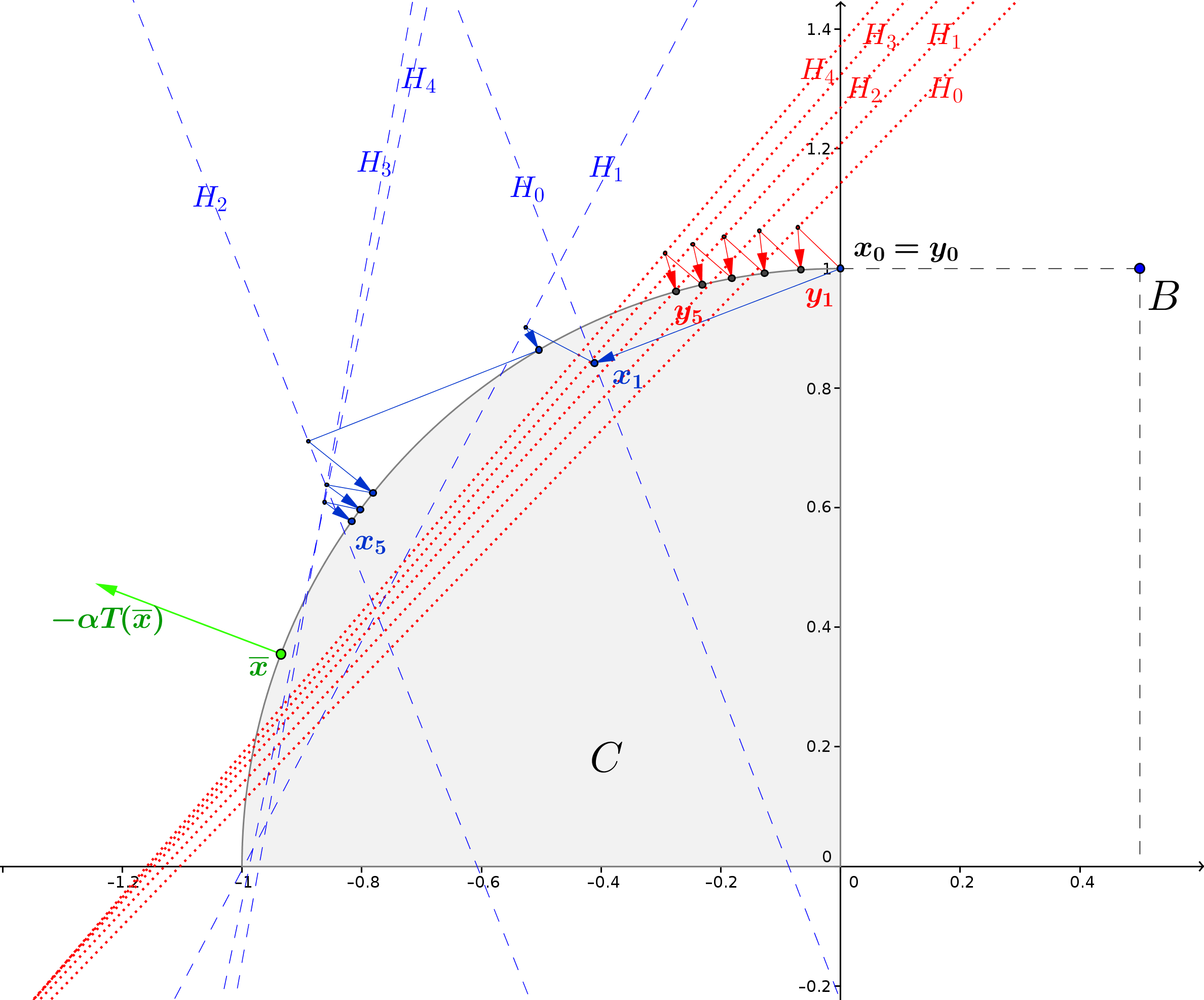
Figure 1: Variant B.1.

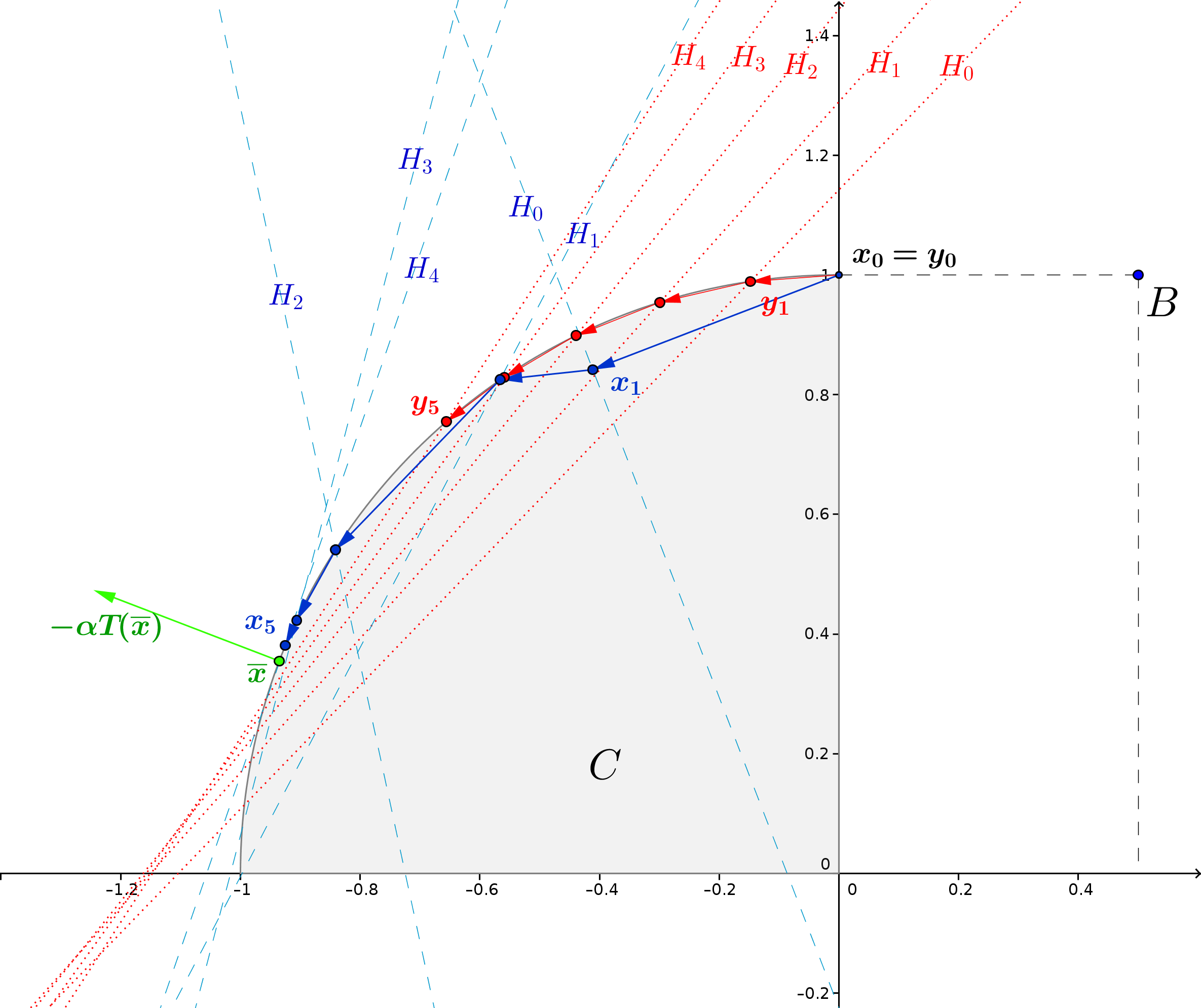
Figure 2: Variant B.2.

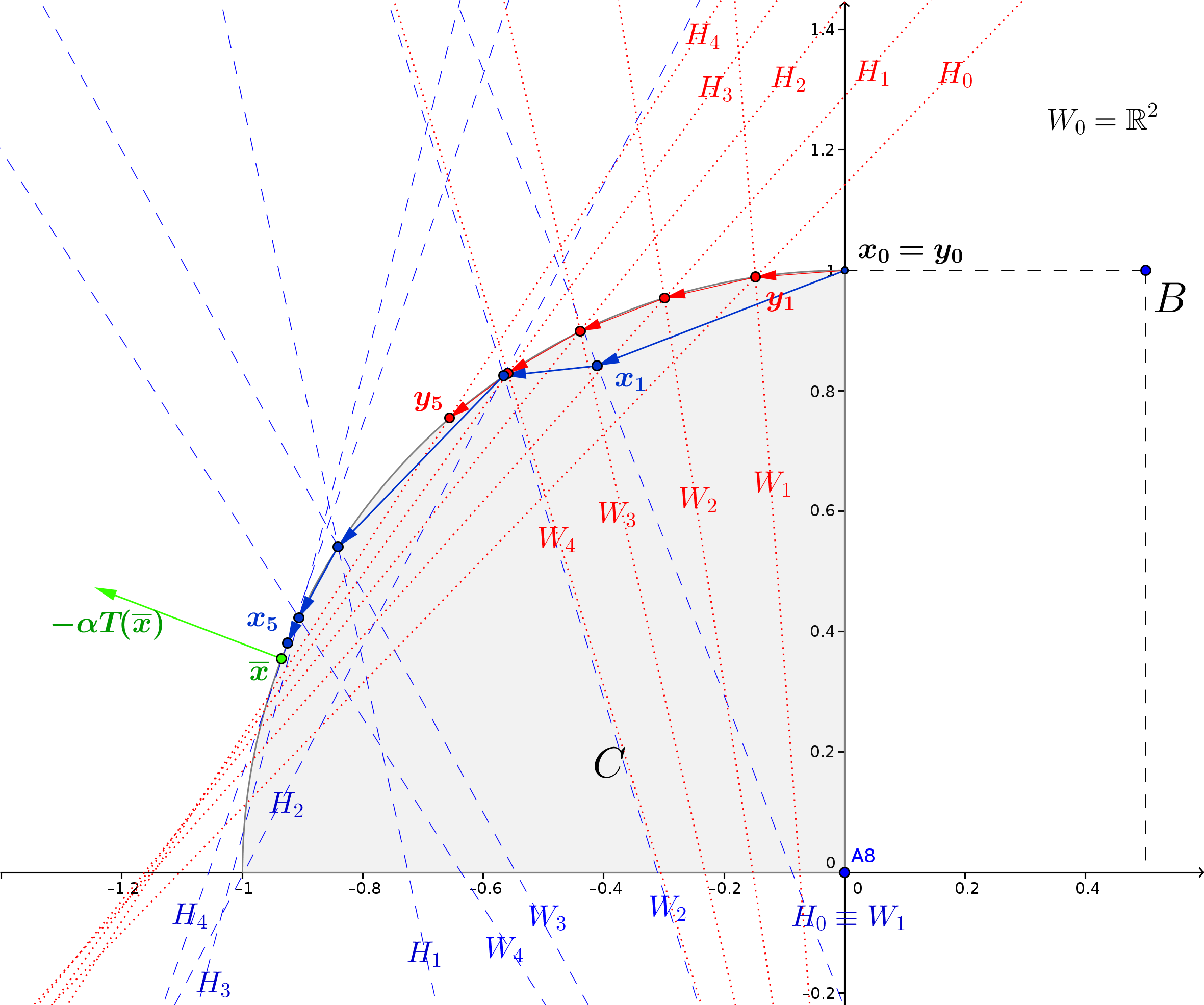
Figure 3: Variant B.3.

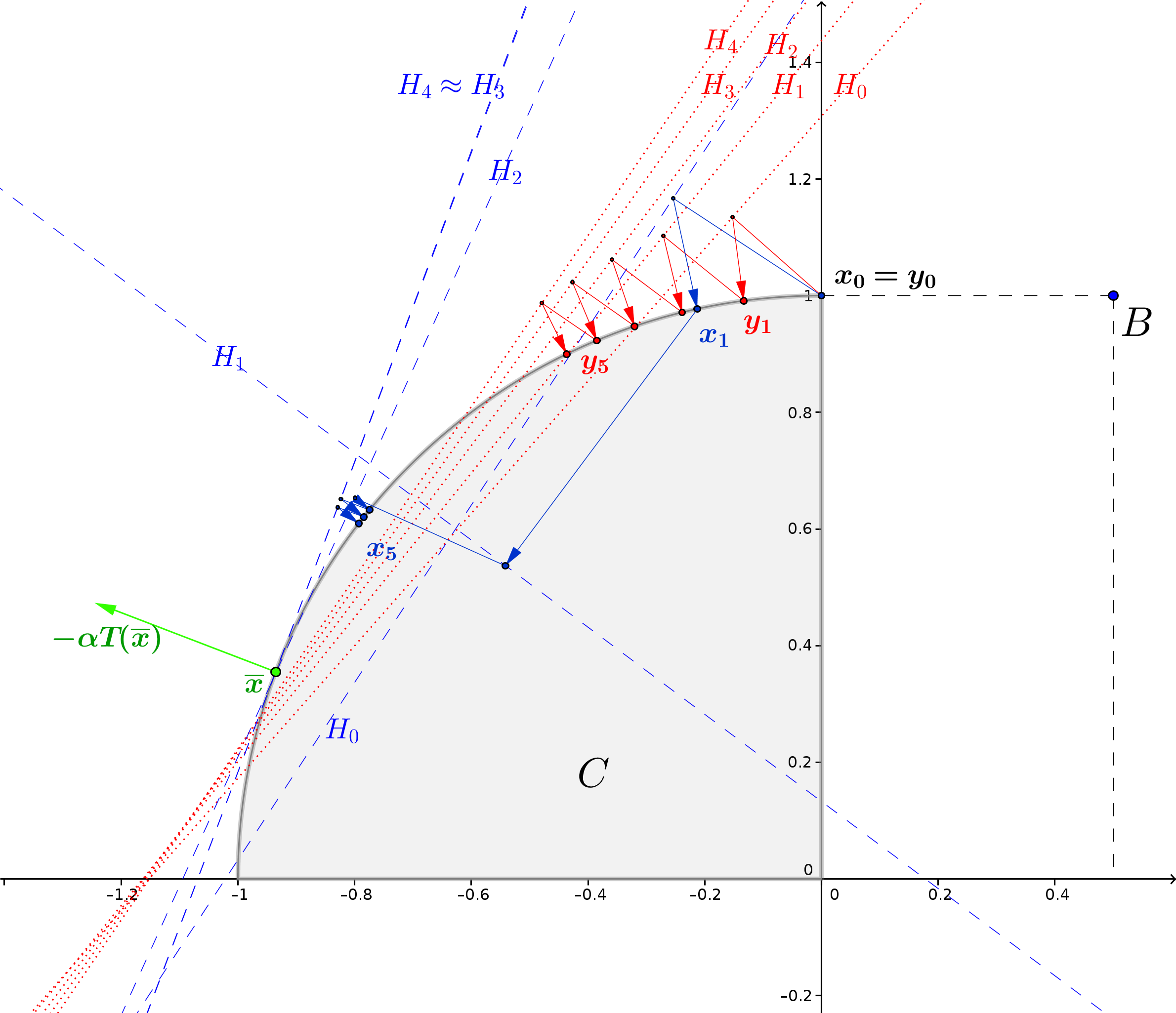
Figure 4: Variant F.1.

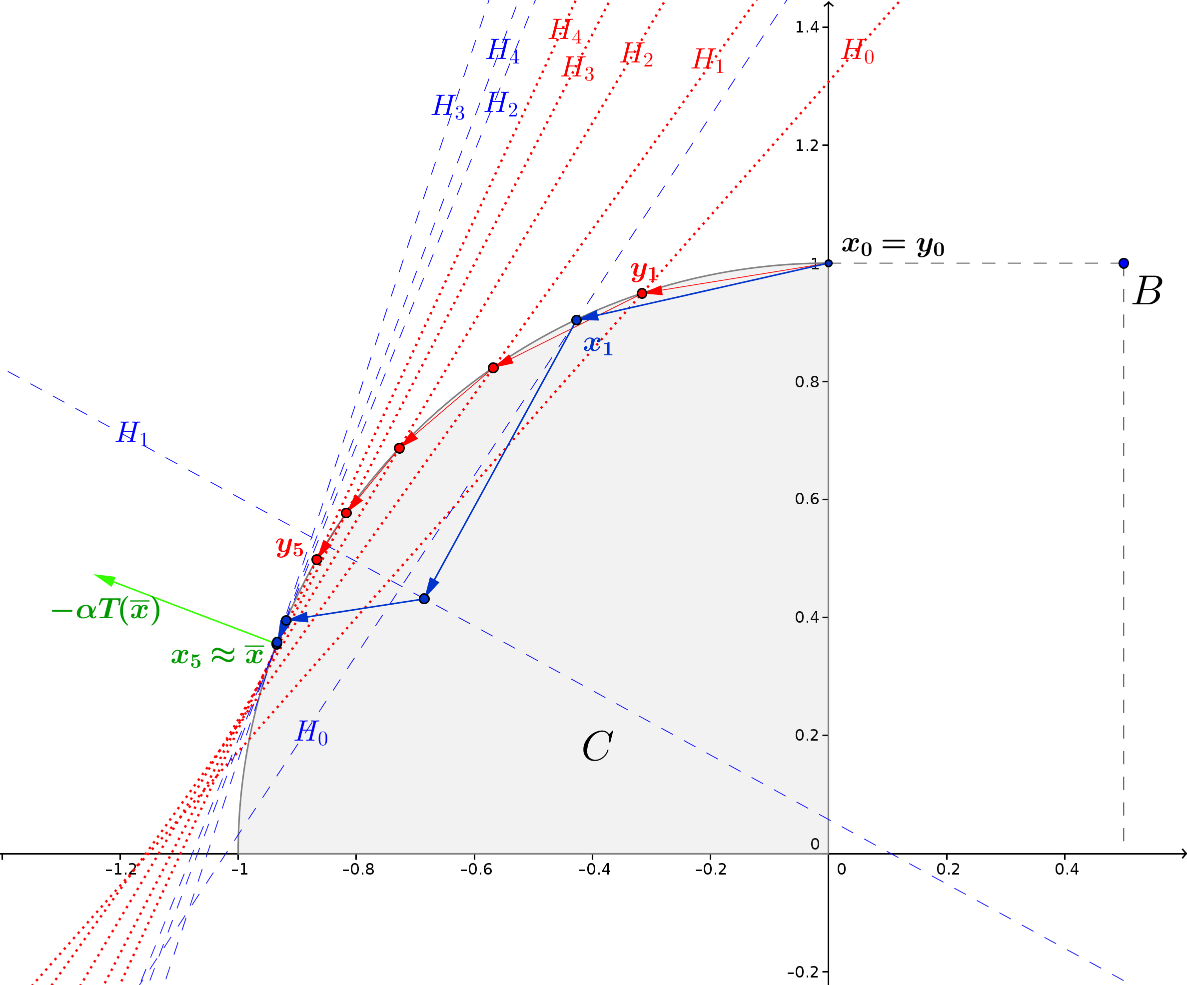
Figure 5: Variant F.2.

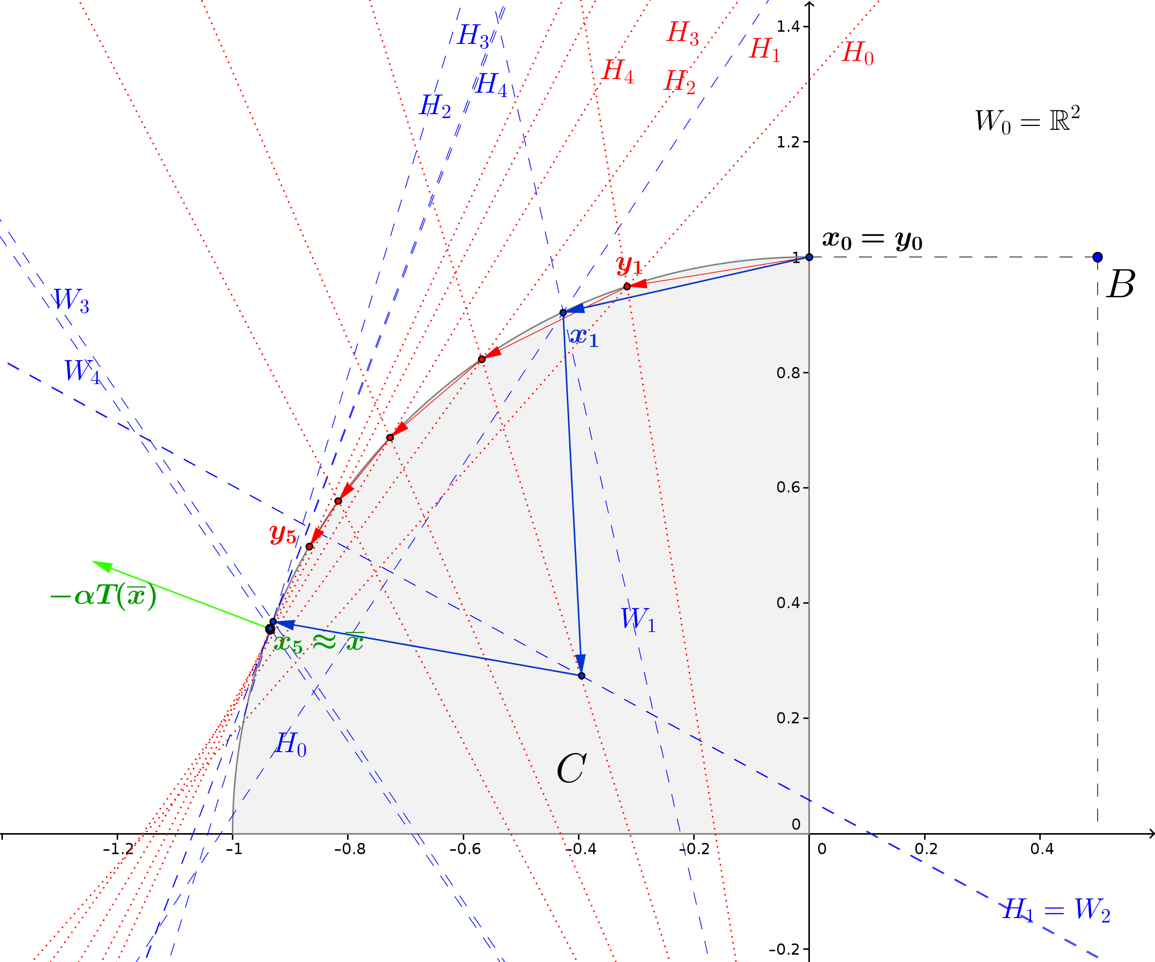
Figure 6: Variant F.3.

The performance suggests that our approach can be used in a hybrid scheme that takes advantage of normal vectors in early iterations.

6 Conclusion

In this paper, we have proposed two conceptual conditional extragradient algorithms that generalize classical extragradient algorithms for solving constrained variational inequality problems (VIP). The main idea is to use nonzero normal vectors to the feasible set to improve the convergence. This approach uses two different linesearches extending several known projection algorithms for VIP. These linesearches allow us to find suitable halfspaces containing the solution set of the problem by using nonzero normal vectors of the feasible set. It is well-known in the literature that such procedures are very effective in absence of Lipschitz continuity exploiting most of the information available at each iteration to produce possibly long steplengths. Convergence results are also established assuming existence of solutions, continuity and a weaker condition than pseudomonotonicity on the operator enlarging the class of VIP that we can solve. This is a humble attempt in targeting more efficient variants which may permit to find the optimal choice of normals on the feasible set.

Several of the ideas of this paper merit further investigation, some of which would be presented in future work. In particular, we are working on variants of the projection algorithms proposed in [6] for solving nonsmooth variational inequalities. The difficulties of extending this previous result to point-to-set operators are non-trivial, the main obstacle lies in the impossibility to use linesearches or separating techniques. To the best of our knowledge, variants of the linesearches for variational inequalities require smoothness of $T$: even for nonsmooth convex optimization problems ($T=\partial f$), it is not possible make linesearch because the negative subgradients are not always descent directions. Actually, a few explicit methods have been proposed in the literature for solving nonsmooth monotone variational inequality problems (see, e.g., [14, 23]). Moreover, future work will address further investigation on the modified Forward-Backward splitting iteration for inclusion problems [4, 5, 39], exploiting the additive structure of the main operator and adding dynamic choices of the stepsizes with conditional and deflected techniques [33, 16].

References

[1] Auslender, A., Teboulle, M.: Interior projection-like methods for monotone variational
inequalities. Math. Program.104 (2005)
39–68.
[2] Bauschke, H.H., Borwein, J.M.: On projection algorithms for solving convex feasibility problems. SIAM Rev.38 (1996) 367–426.
[3] Bauschke, H.H., Combettes, Patrick L.: Convex Analysis and Monotone Operator Theory in Hilbert Spaces. Springer, New York (2011).
[4] Bello Cruz, J.Y., Díaz Millán, R.: A direct splitting method for nonsmooth variational inequalities. J. Optim. Theory Appl.161 (2014) 728–737.
[5] Bello Cruz, J.Y., Díaz Millán, R.:
A variant of Forward-Backward splitting method for the sum of two
monotone operators with a new search strategy. Optimization64 (2015) 1471–1486.
[6] Bello Cruz, J.Y., Díaz Millán, R.:
A relaxed-projection splitting algorithm for variational inequalities in Hilbert spaces. J. Global Optim.65 (2016) 597–614.
[7] Bello Cruz, J.Y., Iusem, A.N.: A strongly convergent direct method for monotone variational inequalities in Hilbert spaces. Numer. Funct. Anal. Optim.30 (2009) 23–36.
[8] Bello Cruz, J.Y., Iusem, A.N.: Convergence of direct methods for paramonotone variational inequalities.
Comput. Optim. Appl.46 (2010)
247–263.
[9] Bello Cruz, J.Y., Iusem, A.N.: A strongly convergent method for nonsmooth convex minimization in Hilbert spaces.
Numer. Funct. Anal. Optim.32 (2011)
1009–1018.
[10] Bello Cruz, J.Y., Iusem, A.N.: An explicit algorithm for monotone variational inequalities. Optimization61 (2012) 855–871.
[11] Bonnans, J.F., Shapiro, A.: Perturbation Analysis
of Optimization Problems. Springer, New York (2000).
[12] Browder, F.E.: Convergence theorems for sequences of nonlinear operators in Banach spaces.
Math. Z.100 (1967) 201–225.
[13] Burachik, R.S., Iusem, A.N.: Set-Valued Mappings and
Enlargements of Monotone Operators. Springer, Berlin (2008).
[14] Burachik, R.S., Lopes, J.O., Svaiter, B.F.: An
outer approximation method for the variational inequality problem.
SIAM J. Control Optim.43 (2005)
2071–2088.
[15] Censor, Y., Gibali, A., Reich, S.: The subgradient extragradient method for solving variational inequalities in Hilbert space.
J. Optim. Theory Appl.148
(2011) 318–335.
[16] d’Antonio, G., Frangioni, A.: Convergence analysis of deflected conditional approximate subgradient methods. SIAM J. Optim.20 (2009) 357–386.
[18] Demyanov, V.F., Vasilyev, L.V.: Nondifferentiable Optimization (Nauka, Moscow, (1981); Engl. transl. in Optimization Software, New York, (1985)).
[19] Facchinei, F., Pang, J.S.: Finite-dimensional Variational Inequalities and Complementarity Problems. Springer, Berlin (2003).
[20] Ferris, M.C., Pang, J.S.: Engineering and economic applications of
complementarity problems. SIAM Rev.39 (1997)
669–713.
[21] Harker, P.T., Pang, J.S.: Finite dimensional variational
inequalities and nonlinear complementarity problems: a survey of
theory, algorithms and applications. Math. Program.48 (1990) 161–220.
[22] Hartman, P., Stampacchia, G.: On some non-linear elliptic differential-functional equations.
Acta Math.115 (1966) 271–310.
[23] He, B.S.: A new method for a class of variational inequalities.
Math. Program.66 (1994) 137–144.
[24] Iusem, A.N.: An iterative algorithm for the variational
inequality problem. Comp. Appl. Math.13 (1994) 103–114.
[25] Iusem, A.N., Svaiter, B.F.: A variant of Korpelevich’s method for variational inequalities with a new search strategy.
Optimization42 (1997) 309–321.
[27] Kinderlehrer, D., Stampacchia, G.: An Introduction to
Variational Inequalities and Their Applications. Academic
Press, New York (1980).
[28] Khobotov, E.N.: Modifications of the extragradient method
for solving variational inequalities and certain optimization
problems. USSR Comput. Math. and Math. Phys.27 (1987) 120–127.
[29] Konnov, I.V.: Combine Relaxation Methods for Variational Inequalities.
Lecture Notes in Economics and Mathematical Systems 495
Springer-Velarg, Berlin (2001).
[30] Konnov, I.V.: A combined relaxation method for variational inequalities with nonlinear constraints. Math. Program.80 (1998) 239–252.
[31] Konnov, I. V.: A class of combined iterative methods for solving variational inequalities.
J. Optim. Theory Appl.94 (1997) 677–693.
[32] Korpelevich, G.M.: The extragradient method for finding saddle
points and other problems. Ekonomika i Matematicheskie Metody12 (1976) 747–756.
[33] Larson, T., Patriksson, M., Stromberg, A-B.:
Conditional subgradient optimization - Theory and application. Eur. J. Oper. Res.88 (1996) 382–403.
[34] Rockafellar, R.T.: Convex Analysis.
Princeton, New York (1970).
[35] Rockafellar, R.T., Wets, R.J-B.: Variational Analysis.
Springer, Berlin (1998).
[36] Solodov, M.V., Svaiter, B.F.: A new projection method
for monotone variational inequality problems. SIAM J. Control Optim.37 (1999) 765–776.
[37] Solodov, M.V., Svaiter, B.F.: Forcing strong convergence of proximal point iterations in a Hilbert space. Math. Program.87 (2000) 189–202.
[38] Solodov, M.V., Tseng, P.: Modified projection-type
methods for monotone variational inequalities. SIAM J. Control Optim.34 (1996) 1814–1830.
[39] Tseng, P.: A modified forward-backward splitting method for maximal monotone mappings. SIAM J. Control Optim.38 (2000) 431–446.
[40] Zaraytonelo, E.H.: Projections on Convex Sets in Hilbert Space and Spectral Theory. in Contributions to
Nonlinear Functional Analysis, E. Zarantonello,
Academic Press, New York (1971) 237–424.