Fast algorithms for Higher-order Singular Value Decomposition
from incomplete data

Abstract

Higher-order singular value decomposition (HOSVD) is an efficient way for data reduction and also eliciting intrinsic structure of multi-dimensional array data. It has been used in many applications, and some of them involve incomplete data. To obtain HOSVD of the data with missing values, one can first impute the missing entries through a certain tensor completion method and then perform HOSVD to the reconstructed data. However, the two-step procedure can be inefficient and does not make reliable decomposition.

In this paper, we formulate an incomplete HOSVD problem and combine the two steps into solving a single optimization problem, which simultaneously achieves imputation of missing values and also tensor decomposition. We also present one algorithm for solving the problem based on block coordinate update (BCU). Global convergence of the algorithm is shown under mild assumptions and implies that of the popular higher-order orthogonality iteration (HOOI) method, and thus we, for the first time, give global convergence of HOOI.

In addition, we compare the proposed method to state-of-the-art ones for solving incomplete HOSVD and also low-rank tensor completion problems and demonstrate the superior performance of our method over other compared ones. Furthermore, we apply it to face recognition and MRI image reconstruction to show its practical performance.

5F99, 9008, 90C06, 90C26.

1 Introduction

Multi-dimensional arrays (or called tensors) appear in many applications that collect data along multiple dimensions, including space, time, and spectrum, from different subjects (e.g., patients), and under different conditions (e.g., view points, illuminations, expressions). Higher-order singular value decomposition (HOSVD) [6] is an efficient way for dimensionality reduction and eliciting the intrinsic structure of the multi-dimensional data. It generalizes the matrix SVD and decomposes a multi-dimensional array into the product of a core tensor and a few orthogonal matrices, each of which captures the subspace information corresponding to one dimension (also called mode or way). The decomposition can be used for classification tasks including face recognition [41], handwritten digit classification [34], human motion analysis and recognition [40], and so on. HOSVD can also be applied to predicting unknown values while the acquired data is incomplete such as seismic data reconstruction [18] and personalized web search [37]. On imputing missing values, data fitting is the main goal instead of decomposition itself. However, there are applications that involve missing values and also require the decomposition such as face recognition [12], facial age estimation [11], and DNA microarray data analysis [28].

In this paper, we aim at finding an approximate HOSVD of a given multi-dimensional array with missing values. More precisely, given partial entries of a tensor $\boldsymbol{{\mathcal{M}}}\in\mathbb{R}^{m_{1}\times\ldots\times m_{N}}$, we estimate its HOSVD as $\boldsymbol{{\mathcal{C}}}\times_{1}{\mathbf{A}}_{1}\ldots\times_{N}{\mathbf{A}}_{N}$ such that the product is close to the underlying tensor $\boldsymbol{{\mathcal{M}}}$ and ${\mathbf{A}}_{n}$ can capture dominant subspace of the $n$-th mode of $\boldsymbol{{\mathcal{M}}}$ for all $n$, where $\boldsymbol{{\mathcal{C}}}\in\mathbb{R}^{r_{1}\times\ldots\times r_{N}}$ is a core tensor, ${\mathbf{A}}_{n}\in\mathbb{R}^{m_{n}\times r_{n}}$ has orthonormal columns for all $n$, and $\times_{n}$ denotes the mode-$n$ tensor-matrix multiplication (see (2) below). To achieve the goal, we propose to solve the following incomplete HOSVD problem:

$$\begin{array}[]{ll}\underset{\boldsymbol{\mathcal{C}},\mathbf{A}}{\min}\,\frac{1}{2}\|\mathcal{P}_{\Omega}(\boldsymbol{\mathcal{C}}\times_{1}\mathbf{A}_{1}\ldots\times_{N}\mathbf{A}_{N}-\boldsymbol{\mathcal{M}})\|_{F}^{2},\\[2.84544pt] \mbox{ s.t. }{\mathbf{A}}_{n}^{\top}{\mathbf{A}}_{n}={\mathbf{I}},\,{\mathbf{A}}_{n}\in\mathbb{R}^{m_{n}\times r_{n}},\,n=1,\ldots,N,\end{array}$$ (1)

where $\mathbf{A}=(\mathbf{A}_{1},\ldots,\mathbf{A}_{N})$, $(r_{1},\ldots,r_{N})$ is a given multilinear rank, ${\mathbf{I}}$ is the identity matrix of appropriate size, $\Omega$ indexes the observed entries, and ${\mathcal{P}}_{\Omega}$ is a projection that keeps the entries in $\Omega$ and zeros out others. Since only partial entries of $\boldsymbol{{\mathcal{M}}}$ are assumed known in (1), we cannot have $r_{n}=m_{n},\,n=1,\ldots,N$, because otherwise, it will cause overfitting problem. Hence, in general, instead of a full HOSVD, we can only get a truncated HOSVD of $\boldsymbol{{\mathcal{M}}}$ from its partial entries.

To get an approximate HOSVD of $\boldsymbol{{\mathcal{M}}}$ from its partial entries, one can also first fill in the unobserved entries through a certain tensor completion method and then perform some iterative method to have a (truncated) HOSVD of the estimated tensor. The advantage of our method is that it combines the two steps into solving just one problem and is usually more efficient and accurate. In addition, upon solving (1), we can also estimate the unobserved entries of $\boldsymbol{{\mathcal{M}}}$ from $\boldsymbol{\mathcal{C}}\times_{1}\mathbf{A}_{1}\ldots\times_{N}\mathbf{A}_{N}$ and thus achieve the tensor completion as a byproduct.

We will write (1) into one equivalent problem and solve it by the block coordinate descent (BCD) method. Although the problem is non-convex, we will demonstrate that (1) solved by the simple BCD can perform better than state-of-the-art tensor completion methods on reconstructing (approximate) low-multilinear-rank tensors. In addition, it can produce more reliable factors and as a result give higher prediction accuracies on certain classification problems such as the face recognition problem.

1.1 Related work

We first review methods for matrix and tensor factorization with missing values and then existing works on low-rank tensor completion (LRTC).

Matrix and tensor factorization with missing values

The matrix SVD from incomplete data has been studied for decades; see [33, 20] for example. It can be regarded as a special case of (1) by setting $N=2$ and restricting $\boldsymbol{{\mathcal{C}}}$ to be a nonnegative diagonal matrix. Further removing the orthogonality constraint on ${\mathbf{A}}_{n}$’s and setting $\boldsymbol{{\mathcal{C}}}$ as the identity matrix, (1) reduces to the matrix factorization from incomplete data (e.g., see [9]). Existing methods for achieving matrix SVD or factorization with missing values are mainly BCD-type ones such as the expectation maximization (EM) in [36] that alternates between imputation of the missing values and SVD computation of the most recently estimated matrix, and the successive over-relaxation (SOR) in [43] that iteratively updates the missing values and the basis and coefficient factors by alternating least squares with extrapolation. There are also approaches that updates all variables simultaneously at each iteration. For example, [4] employs the damped Newton method for matrix factorization with missing values. Usually, the damped Newton method converges faster than BCD-type ones but has much higher per-iteration complexity.

Tensor factorization from incomplete data has also been studied for many years such as the CANDECOMP / PARAFAC (CP) tensor factorization with missing values in [1], the weighted nonnegative CP tensor factorization in [29], the weighted Tucker decomposition in [35, 8], the nonnegative Tucker decomposition with missing data in [26], and the recently proposed Bayesian CP factorization of incomplete tensors in [50]. BCD-type method has also been employed for solving tensor factorization with missing values. For example, [42] use the EM method for Tucker decomposition from incomplete data, [8] uses block coordinate minimization for the weighted Tucker decomposition, and [26] and [44] solve the nonnegative Tucker decomposition with missing data by the multiplicative updating and alternating prox-linearization method, respectively. There are also non-BCD-type methods such as the Gauss-Newton method in [38] and nonlinear conjugate gradient method for CP factorization with missing values, and the damped Newton method in [31] for nonnegative Tucker decomposition.

With all entries observed, (1) becomes the best rank-$(r_{1},\ldots,r_{N})$ approximation problem in [7], where a higher-order orthogonality iteration (HOOI) method is given. Although HOOI often works well, no convergence result has been shown in the literature except that it makes the objective value nonincreasing at the iterates. As a special case of our algorithm (see Algorithm 1 below), we will give its global convergence in terms of a first-order optimality condition.

Although not explicitly formulated, (1) has been used in [12] for face recognition with incomplete training data and in [11] for facial age estimation. Both works achieve the incomplete HOSVD by the EM method which alternates between the imputation of missing values and performing HOOI to the most recently estimated tensor. Our algorithm (see Algorithm 1 below) is similar to the EM method. However, our method performs just one HOOI iteration within each cycle of updating factor matrices instead of running HOOI for many iterations as done in [11, 12], and thus our method has much cheaper per-cycle complexity and faster overall convergence. Another closely related work is [5], which proposes the simultaneous tensor decomposition and completion (STDC) without orthogonality on factor matrices. It makes the core tensor of the same size as the original tensor and square factor matrices. In addition, it models STDC by nuclear norm regularized minimization, which can be much more expensive than (1) to solve.

Low-rank tensor completion

Like (1), all other tensor factorization with missing values can also be used to estimate the unobserved entries of the underlying tensor. When the tensor has some low-rankness property, the estimation can be highly accurate. For example, [8] applies the Tucker factorization with missing data to LRTC and can have fitting error low to the order of $10^{-5}$ for randomly generated low-multilinear-rank tensors. The work [24] employs CP factorization with missing data and also demonstrates that low-multilinear-rank tensors can be reconstructed into high accuracy.

Many other methods for LRTC directly impute the missing entries such that the reconstructed tensor has low-rankness property. The pioneering work [23] proposes to minimize the weighted nuclear norm of all mode matricization (see the definition in section 1.3) of the estimated tensor. Various methods are applied in [23] to the weighted nuclear norm minimization including BCD, the proximal gradient, and the alternating direction method of multiplier (ADMM). The same idea is employed in [10] to general low-multilinear-rank tensor recovery. Recently, [32] uses, as a regularization term, a tight convex relaxation of the average of the ranks of all mode matricization and applies ADMM to solve the proposed model. The work [27] proposes to reshape the underlying tensor into a more “squared” matrix and then minimize the nuclear norm of the reshaped matrix. It is theoretically shown and also numerically demonstrated in [27] that if the underlying tensor has at least four modes, the “squared” method can perform better than the weighted nuclear norm minimization in [23]. Besides convex optimization methods, nonconvex heuristics have also been proposed for LRTC. For example, [19] explicitly constrains the solution in a low-multilinear-rank manifold and employs the Riemannian conjugate gradient to solve the problem, and [45] applies low-rank matrix factorization to each mode matricization of the underlying tensor and proposes a parallel matrix factorization model, which is then solved by alternating least squares method.

1.2 Contributions

We summarize our contributions as follows.

• We give an explicit formulation of the incomplete HOSVD problem. Although the problem has appeared in many applications, it has never been explicitly formulated as an optimization problem, and thus it is not clear that which objective existing methods are pursuing and whether they have convergence results. An explicit formulation uncovers the objective and enables analyzing the existing methods and also designing more efficient and reliable algorithms.

• We also present a novel algorithm for solving the incomplete HOSVD problem based on BCU method. Under some mild assumptions, global convergence of the algorithm is shown in terms of a first-order optimality condition. The convergence result implies, as a special case, that of the popular HOOI heuristic method [7] for finding the best rank-$(r_{1},\ldots,r_{N})$ approximation of a given tensor, and hence we, for the first time, give the global convergence of the HOOI method.

• Numerical experiments are performed to test the ability of the proposed algorithm on recovering the factors of underlying tensors. Compared to the method in [8] for solving Tucker factorization from incomplete data, our algorithm not only is more efficient but also can give more reliable factors. We also test the proposed method on the LRTC problem and demonstrate that our algorithm can outperform state-of-the-art methods in both running time and solution quality.

• In addition, we apply our method to face recognition and MRI image reconstruction problems and demonstrate that it can perform well on both applications.

1.3 Notation and preliminaries

We use bold capital letters ${\mathbf{X}},{\mathbf{Y}},\ldots$ for matrices and bold caligraphical letter $\boldsymbol{{\mathcal{X}}},\boldsymbol{{\mathcal{Y}}},\ldots$ for tensors. ${\mathbf{I}}$ is reserved for the identity matrix and $\mathbf{0}$ for zero matrix, and their dimensions are known from the context. For $n=1,\ldots,N$, we denote ${\mathcal{O}}_{n}=\{{\mathbf{A}}_{n}:\,{\mathbf{A}}_{n}^{\top}{\mathbf{A}}_{n}={\mathbf{I}}\}$ as the manifold of the $n$-th factor matrix. We use $\sigma_{i}({\mathbf{X}})$ to denote the $i$-th largest singular value of ${\mathbf{X}}$. By compact SVD of ${\mathbf{X}}$, we always mean ${\mathbf{X}}={\mathbf{U}}_{x}\boldsymbol{\Sigma}_{x}{\mathbf{V}}_{x}^{\top}$ with $\boldsymbol{\Sigma}_{x}$ having all positive singular values of ${\mathbf{X}}$ on its diagonal and ${\mathbf{U}}_{x}$ and ${\mathbf{V}}_{x}$ containing the corresponding left and right singular vectors. The $(i_{1},\ldots,i_{N})$-th component of an $N$-way tensor $\boldsymbol{\mathcal{X}}$ is denoted as $x_{i_{1}\ldots i_{N}}$. For $\boldsymbol{\mathcal{X}},\boldsymbol{\mathcal{Y}}\in\mathbb{R}^{m_{1}\times\ldots\times m_{N}}$, their inner product is defined in the same way as that for matrices, i.e.,

$$\langle\boldsymbol{\mathcal{X}},\boldsymbol{\mathcal{Y}}\rangle=\sum_{i_{1}=1}^{m_{1}}\cdots\sum_{i_{N}=1}^{m_{N}}x_{i_{1}\ldots i_{N}}\cdot y_{i_{1}\ldots i_{N}}.$$

The Frobenius norm of $\boldsymbol{\mathcal{X}}$ is defined as $\|\boldsymbol{\mathcal{X}}\|_{F}=\sqrt{\langle\boldsymbol{\mathcal{X}},\boldsymbol{\mathcal{X}}\rangle}.$

We review some basic concepts about tensor below. For more details, the readers are referred to [17].

A fiber of $\boldsymbol{\mathcal{X}}$ is a vector obtained by fixing all indices of $\boldsymbol{\mathcal{X}}$ except one, and a slice of $\boldsymbol{\mathcal{X}}$ is a matrix by fixing all indices of $\boldsymbol{\mathcal{X}}$ except two. The vectorization of $\boldsymbol{{\mathcal{X}}}$ gives a vector, which is obtained by stacking all mode-1 fibers of $\boldsymbol{{\mathcal{X}}}$ and denoted by ${\mathrm{vec}}(\boldsymbol{{\mathcal{X}}})$. The mode-$n$ matricization (also called unfolding) of $\boldsymbol{\mathcal{X}}$ is denoted as $\mathbf{X}_{(n)}$ or ${\mathbf{unfold}}_{n}(\boldsymbol{{\mathcal{X}}})$, which is a matrix with columns being the mode-$n$ fibers of $\boldsymbol{\mathcal{X}}$ in the lexicographical order, and we define ${\mathbf{fold}}_{n}$ to reverse the process, i.e., ${\mathbf{fold}}_{n}({\mathbf{unfold}}_{n}(\boldsymbol{\mathcal{X}}))=\boldsymbol{\mathcal{X}}$. The mode-$n$ product of $\boldsymbol{\mathcal{X}}\in\mathbb{R}^{m_{1}\times\cdots\times m_{N}}$ with $\mathbf{B}\in\mathbb{R}^{p\times m_{n}}$ is written as $\boldsymbol{\mathcal{X}}\times_{n}\mathbf{B}$ which gives a tensor in $\mathbb{R}^{n_{1}\times\cdots\times m_{n-1}\times p\times m_{n+1}\times\cdots\times m_{N}}$ and is defined component-wisely by

$$(\boldsymbol{\mathcal{X}}\times_{n}\mathbf{B})_{i_{1}\cdots i_{n-1}ji_{n+1}\cdots i_{N}}=\sum_{i_{n}=1}^{m_{n}}x_{i_{1}i_{2}\cdots i_{N}}\cdot b_{ji_{n}}.$$ (2)

For any tensor $\boldsymbol{{\mathcal{G}}}$ and matrices ${\mathbf{X}}$ and ${\mathbf{Y}}$ of appropriate size, it holds

$$\boldsymbol{{\mathcal{G}}}\times_{n}({\mathbf{X}}{\mathbf{Y}})=(\boldsymbol{{\mathcal{G}}}\times_{n}{\mathbf{Y}})\times_{n}{\mathbf{X}},\,\forall n.$$ (3)

If $\boldsymbol{\mathcal{X}}=\boldsymbol{\mathcal{C}}\times_{i=1}^{N}\mathbf{A}_{i}:=\boldsymbol{\mathcal{C}}\times_{1}\mathbf{A}_{1}\cdots\times_{N}\mathbf{A}_{N}$, then

$$\mathbf{X}_{(n)}=\mathbf{A}_{n}\mathbf{C}_{(n)}\left(\otimes_{\begin{subarray}{c}i=N\\ i\neq n\end{subarray}}^{1}\mathbf{A}_{i}\right)^{\top},\,\forall n.$$ (4)

and

$${\mathrm{vec}}(\boldsymbol{\mathcal{X}})=\left(\otimes_{n=N}^{1}\mathbf{A}_{n}\right){\mathrm{vec}}(\boldsymbol{\mathcal{C}}),$$ (5)

where

$$\otimes_{n=N}^{1}\mathbf{A}_{n}:=\mathbf{A}_{N}\otimes\cdots\otimes\mathbf{A}_{1},$$ (6)

and $\mathbf{A}\otimes\mathbf{B}$ denotes Kronecker product of $\mathbf{A}$ and $\mathbf{B}$.

For any matrices ${\mathbf{A}}$, ${\mathbf{B}}$, ${\mathbf{C}}$ and ${\mathbf{D}}$ of appropriate size, we have (c.f. [15, Chapter 4])

$$\mathbf{A}\otimes\mathbf{B}\otimes\mathbf{C}=(\mathbf{A}\otimes\mathbf{B})\otimes\mathbf{C}=\mathbf{A}\otimes(\mathbf{B}\otimes\mathbf{C}),$$ (7a)

$$(\mathbf{A}\otimes\mathbf{B})(\mathbf{C}\otimes\mathbf{D})=(\mathbf{A}\mathbf{C})\otimes(\mathbf{B}\mathbf{D}),$$ (7b)

$$(\mathbf{A}\otimes\mathbf{B})^{\top}=\mathbf{A}^{\top}\otimes\mathbf{B}^{\top},$$ (7c)

$$(\mathbf{A}\otimes\mathbf{B})^{\dagger}=\mathbf{A}^{\dagger}\otimes\mathbf{B}^{\dagger},$$ (7d)

where ^† denotes the Moore-Penrose pseudo-inverse.

1.4 Outline

The rest of the paper is organized as follows. In section 2, we write (1) into one equivalent problem and present an algorithm based on BCU. Convergence analysis of the algorithm is given in section 3, and numerical results are presented in section 4. Finally, section 5 concludes the paper.

2 Algorithm

In this section, we write (1) into one equivalent problem and apply the BCU method to it. We choose BCU because of the problem’s nice structure, which enables BCU to be more efficient than full coordinate update method; see [30]. Convergence analysis of the algorithm will be given in next section.

2.1 Alternative formulation

Introducing auxiliary variable $\boldsymbol{\mathcal{X}}$, we write (1) into the following equivalent problem

$$\begin{array}[]{ll}\underset{\boldsymbol{\mathcal{C}},\mathbf{A},\boldsymbol{\mathcal{X}}}{\min}\,f(\boldsymbol{\mathcal{C}},\mathbf{A},\boldsymbol{\mathcal{X}})\equiv\frac{1}{2}\|\boldsymbol{\mathcal{C}}\times_{1}\mathbf{A}_{1}\ldots\times_{N}\mathbf{A}_{N}-\boldsymbol{\mathcal{X}}\|_{F}^{2},\\[2.84544pt] \mbox{ s.t. }{\mathbf{A}}_{n}^{\top}{\mathbf{A}}_{n}={\mathbf{I}},\,{\mathbf{A}}_{n}\in\mathbb{R}^{m_{n}\times r_{n}},\,n=1,\ldots,N,\,\mathcal{P}_{\Omega}(\boldsymbol{\mathcal{X}})=\mathcal{P}_{\Omega}(\boldsymbol{\mathcal{M}}).\end{array}$$ (8)

The equivalence between (1) and (8) can be easily seen by setting ${\mathcal{P}}_{\Omega^{c}}(\boldsymbol{{\mathcal{X}}})={\mathcal{P}}_{\Omega^{c}}(\boldsymbol{\mathcal{C}}\times_{1}\mathbf{A}_{1}\ldots\times_{N}\mathbf{A}_{N})$ in (8). This transformation is similar to those in [43, 22, 47] for low-rank matrix factorization with missing values and also to the EM method in [42] for CP factorization from incomplete data. The objective of (8) is block multi-convex, and one can apply the alternating least squares (ALS) method to it. The ALS method is also new for finding a solution to (1). However, we will focus on another algorithm and present the ALS method in Appendix A.

Note that with ${\mathbf{A}}$ and $\boldsymbol{{\mathcal{X}}}$ fixed in (8), the optimal $\boldsymbol{{\mathcal{C}}}$ is given by

$$\boldsymbol{{\mathcal{C}}}=\boldsymbol{{\mathcal{X}}}\times_{1}{\mathbf{A}}_{1}^{\top}\ldots\times_{N}{\mathbf{A}}_{N}^{\top},$$

and thus one can eliminate $\boldsymbol{{\mathcal{C}}}$ by plugging in the above formula to (8) and have the following equivalent problem

$$\begin{array}[]{ll}\underset{\mathbf{A},\boldsymbol{\mathcal{X}}}{\min}\,g(\mathbf{A},\boldsymbol{\mathcal{X}})\equiv\frac{1}{2}\|\boldsymbol{{\mathcal{X}}}\times_{1}\mathbf{A}_{1}{\mathbf{A}}_{1}^{\top}\ldots\times_{N}\mathbf{A}_{N}{\mathbf{A}}_{N}^{\top}-\boldsymbol{\mathcal{X}}\|_{F}^{2},\\[2.84544pt] \mbox{ s.t. }{\mathbf{A}}_{n}^{\top}{\mathbf{A}}_{n}={\mathbf{I}},\,{\mathbf{A}}_{n}\in\mathbb{R}^{m_{n}\times r_{n}},\,n=1,\ldots,N,\,\mathcal{P}_{\Omega}(\boldsymbol{\mathcal{X}})=\mathcal{P}_{\Omega}(\boldsymbol{\mathcal{M}}).\end{array}$$ (9)

The transformation from (8) to (9) is similar to that employed by the HOOI method in [7] for finding the best rank-$(r_{1},\ldots,r_{N})$ of a given tensor.

2.2 Incomplete HOOI

As what is done in the HOOI method, we propose to alternatingly update ${\mathbf{A}}_{1},\ldots,{\mathbf{A}}_{N}$ and $\boldsymbol{{\mathcal{X}}}$ by minimizing $g$ with respect to one of them while the remaining variables are fixed, one at a time. Specifically, let $(\hat{{\mathbf{A}}}_{1},\ldots,\hat{{\mathbf{A}}}_{N},\hat{\boldsymbol{{\mathcal{X}}}})$ be the current values of the variables and satisfy the feasibility constraints. We renew them to $(\tilde{{\mathbf{A}}}_{1},\ldots,\tilde{{\mathbf{A}}}_{N},\tilde{\boldsymbol{{\mathcal{X}}}})$ through the following updates

$$\tilde{{\mathbf{A}}}_{n}=\operatorname*{arg\,min}_{{\mathbf{A}}_{n}^{\top}{\mathbf{A}}_{n}={\mathbf{I}}}g(\tilde{{\mathbf{A}}}_{<n},{\mathbf{A}}_{n},\hat{{\mathbf{A}}}_{>n},\hat{\boldsymbol{{\mathcal{X}}}}),\,n=1,\ldots,N,$$ (10a)

$$\tilde{\boldsymbol{{\mathcal{X}}}}=\operatorname*{arg\,min}_{{\mathcal{P}}_{\Omega}(\boldsymbol{{\mathcal{X}}})={\mathcal{P}}_{\Omega}(\boldsymbol{{\mathcal{M}}})}g(\tilde{{\mathbf{A}}},\boldsymbol{{\mathcal{X}}}).$$ (10b)

${\mathbf{A}}$-subproblems

Note that if ${\mathbf{A}}_{n}^{\top}{\mathbf{A}}_{n}={\mathbf{I}},\forall n$, then

$$\|\boldsymbol{{\mathcal{X}}}\times_{1}\mathbf{A}_{1}{\mathbf{A}}_{1}^{\top}\ldots\times_{N}\mathbf{A}_{N}{\mathbf{A}}_{N}^{\top}-\boldsymbol{\mathcal{X}}\|_{F}^{2}=\|\boldsymbol{{\mathcal{X}}}\|_{F}^{2}-\|\boldsymbol{{\mathcal{X}}}\times_{1}{\mathbf{A}}_{1}^{\top}\ldots\times_{N}{\mathbf{A}}_{N}^{\top}\|_{F}^{2}.$$ (11)

Hence, from (4), the update of ${\mathbf{A}}_{n}$ in (10a) can be written as

$$\tilde{{\mathbf{A}}}_{n}=\operatorname*{arg\,max}_{{\mathbf{A}}_{n}^{\top}{\mathbf{A}}_{n}={\mathbf{I}}}\|{\mathbf{A}}_{n}^{\top}\hat{{\mathbf{G}}}_{n}\|_{F}^{2},$$ (12)

where $\hat{{\mathbf{G}}}_{n}={\mathbf{unfold}}_{n}(\hat{\boldsymbol{{\mathcal{X}}}}\times_{i=1}^{n-1}\tilde{{\mathbf{A}}}_{i}^{\top}\times_{i=n+1}^{N}\hat{{\mathbf{A}}}_{i}^{\top})$ . Let ${\mathbf{U}}_{n}$ be the matrix containing the left $r_{n}$ leading singular vectors of $\hat{{\mathbf{G}}}_{n}$. Then $\tilde{{\mathbf{A}}}_{n}={\mathbf{U}}_{n}$ solves (12). Note that for any orthogonal matrix ${\mathbf{Q}}_{n}$, ${\mathbf{U}}_{n}{\mathbf{Q}}_{n}$ is also a solution of (12), and the observation will play an important role in the convergence analysis of the proposed algorithm in section 3.

$\boldsymbol{{\mathcal{X}}}$-subproblem

The problem in (10b) can be reduced to solving a normal equation. However, the equation can be extremely large and expensive to solve by a direct method or even an iterative solver for linear system. We propose to approximately solve (10b) by the gradient descent method. Splitting $\boldsymbol{{\mathcal{X}}}={\mathcal{P}}_{\Omega^{c}}(\boldsymbol{{\mathcal{X}}})+{\mathcal{P}}_{\Omega}(\boldsymbol{{\mathcal{M}}})$ and using (11), we write (10b) equivalently into

$$\min_{\boldsymbol{{\mathcal{X}}}}h(\boldsymbol{{\mathcal{X}}};\tilde{{\mathbf{A}}})\equiv\frac{1}{2}\|{\mathcal{P}}_{\Omega^{c}}(\boldsymbol{{\mathcal{X}}})\|_{F}^{2}-\frac{1}{2}\|{\mathcal{P}}_{\Omega^{c}}(\boldsymbol{{\mathcal{X}}})\times_{i=1}^{N}\tilde{{\mathbf{A}}}_{i}^{\top}+{\mathcal{P}}_{\Omega}(\boldsymbol{{\mathcal{M}}})\times_{i=1}^{N}\tilde{{\mathbf{A}}}_{i}^{\top}\|_{F}^{2}.$$ (13)

Since ${\mathcal{P}}_{\Omega}(\hat{\boldsymbol{{\mathcal{X}}}})={\mathcal{P}}_{\Omega}(\boldsymbol{{\mathcal{M}}})$, it is not difficult to show (see Appendix B)

$$\nabla_{\boldsymbol{{\mathcal{X}}}}h(\hat{\boldsymbol{{\mathcal{X}}}};\tilde{{\mathbf{A}}})={\mathcal{P}}_{\Omega^{c}}(\hat{\boldsymbol{{\mathcal{X}}}})-{\mathcal{P}}_{\Omega^{c}}(\hat{\boldsymbol{{\mathcal{X}}}}\times_{i=1}^{N}\tilde{{\mathbf{A}}}_{i}\tilde{{\mathbf{A}}}_{i}^{\top}).$$ (14)

According to the next lemma and [2, Theorem 3.1], one can solve (13) or equivalently (10b) by iteratively updating $\boldsymbol{{\mathcal{X}}}$ through (starting from $\tilde{\boldsymbol{{\mathcal{X}}}}=\hat{\boldsymbol{{\mathcal{X}}}}$)

$$\tilde{\boldsymbol{{\mathcal{X}}}}\leftarrow{\mathcal{P}}_{\Omega^{c}}(\tilde{\boldsymbol{{\mathcal{X}}}}\times_{i=1}^{N}\tilde{{\mathbf{A}}}_{i}\tilde{{\mathbf{A}}}_{i}^{\top})+{\mathcal{P}}_{\Omega}(\boldsymbol{{\mathcal{M}}}).$$ (15)

Lemma 2.1.

If ${\mathbf{A}}_{n}^{\top}{\mathbf{A}}_{n}={\mathbf{I}},\,\forall n$, then $h(\boldsymbol{{\mathcal{X}}};{\mathbf{A}})$ defined in (13) is convex with respect to $\boldsymbol{{\mathcal{X}}}$, and $\nabla_{\boldsymbol{{\mathcal{X}}}}h(\boldsymbol{{\mathcal{X}}};{\mathbf{A}})$ is Lipschitz continuous with constant one, i.e.,

$$\|\nabla_{\boldsymbol{{\mathcal{X}}}}h(\hat{\boldsymbol{{\mathcal{X}}}};{\mathbf{A}})-\nabla_{\boldsymbol{{\mathcal{X}}}}h(\hat{\boldsymbol{{\mathcal{Y}}}};{\mathbf{A}})\|_{F}\leq\|\hat{\boldsymbol{{\mathcal{X}}}}-\hat{\boldsymbol{{\mathcal{Y}}}}\|_{F},\,\forall\hat{\boldsymbol{{\mathcal{X}}}},\hat{\boldsymbol{{\mathcal{Y}}}}.$$

Numerically, we observe that performing just one update in (15) is enough to make sufficient decrease of the objective and the algorithm can converge surprisingly fast. Therefore, we perform only one update in (15) to $\boldsymbol{{\mathcal{X}}}$, and that is exactly letting

$$\tilde{\boldsymbol{{\mathcal{X}}}}=\operatorname*{arg\,min}_{{\mathcal{P}}_{\Omega}(\boldsymbol{{\mathcal{X}}})={\mathcal{P}}_{\Omega}(\boldsymbol{{\mathcal{M}}})}\|\boldsymbol{{\mathcal{X}}}-\hat{\boldsymbol{{\mathcal{X}}}}\times_{i=1}^{N}\tilde{{\mathbf{A}}}_{i}\tilde{{\mathbf{A}}}_{i}^{\top}\|_{F}^{2}.$$ (16)

The pseudocode of the resulting method for solving (9) is shown in Algorithm 1.

Algorithm 1 Incomplete higher-order orthogonality iteration (iHOOI)

1:  Input: index set $\Omega$, observed entries $\mathcal{P}_{\Omega}(\boldsymbol{\mathcal{M}})$, and initial point $(\mathbf{A}^{0},\boldsymbol{\mathcal{X}}^{0})$ with $({\mathbf{A}}_{i}^{0})^{\top}{\mathbf{A}}_{i}^{0}={\mathbf{I}},\forall i$ and $\mathcal{P}_{\Omega}(\boldsymbol{\mathcal{X}}^{0})=\mathcal{P}_{\Omega}(\boldsymbol{\mathcal{M}})$.

2:  for $k=0,1,\ldots$ do

3:     for $n=1,\ldots,N$ do

4:        Let ${\mathbf{A}}_{n}^{k+1}$ be the matrix containing the left $r_{n}$ leading singular vectors of ${\mathbf{G}}_{n}^{k}$ where

$${\mathbf{G}}_{n}^{k}={\mathbf{unfold}}_{n}(\boldsymbol{{\mathcal{X}}}^{k}\times_{i=1}^{n-1}({\mathbf{A}}_{i}^{k+1})^{\top}\times_{i=n+1}^{N}({\mathbf{A}}_{i}^{k})^{\top}).$$ (17)

5:     end for

6:     Update the entries of $\boldsymbol{{\mathcal{X}}}$ not in $\Omega$ by

$${\mathcal{P}}_{\Omega^{c}}(\boldsymbol{\mathcal{X}}^{k+1})={\mathcal{P}}_{\Omega^{c}}\left(\boldsymbol{\mathcal{X}}^{k}\times_{i=1}^{N}\big{(}{\mathbf{A}}_{i}^{k+1}({\mathbf{A}}_{i}^{k+1})^{\top}\big{)}\right).$$ (18)

7:     if stopping criterion is satisfied then

8:        Let $\boldsymbol{{\mathcal{C}}}=\boldsymbol{{\mathcal{X}}}^{k+1}\times_{i=1}^{N}({\mathbf{A}}_{i}^{k+1})^{\top}$ and return $(\boldsymbol{\mathcal{C}},\mathbf{A}^{k+1},\boldsymbol{\mathcal{X}}^{k+1})$.

9:     end if

10:  end for

Remark 2.2 (Comparison between Algorithms 1 and 2).

Since $\boldsymbol{{\mathcal{C}}}$ is absorbed into the update of ${\mathbf{A}}$ and $\boldsymbol{{\mathcal{X}}}$ in Algorithm 1, we expect that it would perform no worse than Algorithm 2 for solving (1) in terms of convergence speed and solution quality and will demonstrate it in section 4 (e.g., see Tables 1 and 2). However, notice that the update of ${\mathbf{A}}_{n}$ in Algorithm 1 typically requires SVD of ${\mathbf{G}}_{n}^{k}$ and can be expensive if $m_{n}$ and $\Pi_{i\neq n}r_{i}$ are both large (e.g., see the test in secion 4.4).

Remark 2.3 (Differences between Algorithm 1 and EM methods in the literature).

Algorithm 1 is very similar to some existing EM methods such as those in [42, 11, 12]. The EM method in [42] is somehow a mixture of Algorithm 1 and Algorithm 2 in Appendix A. Its ${\mathbf{A}}$-updates are the same as those in Algorithm 1 while its $\boldsymbol{{\mathcal{X}}}$-update is the same as that in Algorithm 2. The difference between Algorithm 1 and the methods in [11, 12] is that within each “for” loop, the latter methods perform ${\mathbf{A}}$-updates iteratively to get a rank-$(r_{1},\ldots,r_{N})$ approximation of the estimated $\boldsymbol{{\mathcal{X}}}$.

2.3 Extension

One generalization to the incomplete HOSVD is to find the HOSVD of an underlying tensor $\boldsymbol{{\mathcal{M}}}$ from its underdetermined measurements ${\mathcal{L}}(\boldsymbol{{\mathcal{M}}})$, where ${\mathcal{L}}$ is a linear operator with adjoint ${\mathcal{L}}^{*}$. For this scenario, one can consider to solve the problem

$$\begin{array}[]{ll}\underset{\boldsymbol{\mathcal{X}},\mathbf{A}}{\min}\,\|\boldsymbol{\mathcal{X}}\times_{1}\mathbf{A}_{1}{\mathbf{A}}_{1}^{\top}\ldots\times_{N}\mathbf{A}_{N}{\mathbf{A}}_{N}^{\top}-\boldsymbol{\mathcal{X}}\|_{F}^{2},\\[2.84544pt] \mbox{ s.t. }{\mathbf{A}}_{n}^{\top}{\mathbf{A}}_{n}={\mathbf{I}},\,{\mathbf{A}}_{n}\in\mathbb{R}^{m_{n}\times r_{n}},\,n=1,\ldots,N,\ {\mathcal{L}}(\boldsymbol{{\mathcal{X}}})={\mathcal{L}}(\boldsymbol{{\mathcal{M}}}).\end{array}$$ (19)

A simple modification of Algorithm 1 suffices to handle (19) by using the same ${\mathbf{A}}$-updates in (12) and changing the $\boldsymbol{{\mathcal{X}}}$-update in (16) to

$$\tilde{\boldsymbol{{\mathcal{X}}}}=\operatorname*{arg\,min}_{{\mathcal{L}}(\boldsymbol{{\mathcal{X}}})={\mathcal{L}}(\boldsymbol{{\mathcal{M}}})}\|\boldsymbol{{\mathcal{X}}}-\hat{\boldsymbol{{\mathcal{X}}}}\times_{i=1}^{N}\tilde{{\mathbf{A}}}_{i}\tilde{{\mathbf{A}}}_{i}^{\top}\|_{F}^{2},$$

which is equivalent to letting

$$\tilde{\boldsymbol{{\mathcal{X}}}}=\hat{\boldsymbol{{\mathcal{X}}}}\times_{i=1}^{N}\tilde{{\mathbf{A}}}_{i}\tilde{{\mathbf{A}}}_{i}^{\top}+{\mathcal{L}}^{*}({\mathcal{L}}{\mathcal{L}}^{*})^{-1}({\mathcal{L}}(\boldsymbol{{\mathcal{M}}})-{\mathcal{L}}(\hat{\boldsymbol{{\mathcal{X}}}}\times_{i=1}^{N}\tilde{{\mathbf{A}}}_{i}\tilde{{\mathbf{A}}}_{i}^{\top})).$$

From the above update, we see that to make the modified algorithm efficient, the evaluation of ${\mathcal{L}},{\mathcal{L}}^{*}$ and $({\mathcal{L}}{\mathcal{L}}^{*})^{-1}$ needs be cheap such as ${\mathcal{L}}={\mathcal{P}}_{\Omega}$ in the incomplete HOSVD and ${\mathcal{L}}$ being a partial Fourier transformation considered in [10] for low-rank tensor recovery.

3 Convergence Analysis

In this section, we analyze the convergence of Algorithm 1. We show its global convergence in terms of the first-order optimality condition of (8). The main assumption we make is a condition (see (27)) similar to that made by the orthogonal iteration method (c.f. [14, section 7.3.2]) for computing $r$-dimensional dominant invariant subspace of a matrix.

3.1 First-order optimality conditions

The Lagrangian function of (9) is

$${\mathcal{L}}_{g}({\mathbf{A}},\boldsymbol{{\mathcal{X}}},\boldsymbol{\Lambda},\boldsymbol{{\mathcal{Y}}})=g({\mathbf{A}},\boldsymbol{{\mathcal{X}}})+\frac{1}{2}\sum_{n=1}^{N}\langle\boldsymbol{\Lambda}_{n},{\mathbf{A}}_{n}^{\top}{\mathbf{A}}_{n}-{\mathbf{I}}\rangle+\langle\boldsymbol{{\mathcal{Y}}},{\mathcal{P}}_{\Omega}(\boldsymbol{{\mathcal{X}}})-{\mathcal{P}}_{\Omega}(\boldsymbol{{\mathcal{M}}})\rangle,$$

where $\boldsymbol{\Lambda}=(\boldsymbol{\Lambda}_{1},\ldots,\boldsymbol{\Lambda}_{N})$ and $\boldsymbol{{\mathcal{Y}}}$ are Lagrangian multipliers, and $\boldsymbol{\Lambda}_{n}$’s are symmetric matrices. Letting $\nabla{\mathcal{L}}_{g}=\mathbf{0}$, we derive the KKT conditions of (9) to be

$${\mathbf{G}}_{n}{\mathbf{G}}_{n}^{\top}{\mathbf{A}}_{n}-{\mathbf{A}}_{n}\boldsymbol{\Lambda}_{n}= \,\mathbf{0},\,n=1,\ldots,N,$$ (20a)

$$\boldsymbol{{\mathcal{X}}}-\boldsymbol{{\mathcal{X}}}\times_{i=1}^{N}{\mathbf{A}}_{i}{\mathbf{A}}_{i}^{\top}+{\mathcal{P}}_{\Omega}(\boldsymbol{{\mathcal{Y}}})= \,\mathbf{0},$$ (20b)

$${\mathbf{A}}_{n}^{\top}{\mathbf{A}}_{n}-{\mathbf{I}}= \,\mathbf{0},\,n=1,\ldots,N,$$ (20c)

$${\mathcal{P}}_{\Omega}(\boldsymbol{{\mathcal{X}}})-{\mathcal{P}}_{\Omega}(\boldsymbol{{\mathcal{M}}})= \,\mathbf{0},$$ (20d)

where

$${\mathbf{G}}_{n}={\mathbf{unfold}}_{n}\big{(}\boldsymbol{{\mathcal{X}}}\times_{i=1}^{n-1}{\mathbf{A}}_{i}^{\top}\times_{i=n+1}^{N}{\mathbf{A}}_{i}^{\top}\big{)}.$$

From [3, Proposition 3.1.1], we have that any local minimizer of (9) satisfies the conditions in (20). Due to nonconvexity of (9), we cannot in general guarantee global optimality, so instead we aim at showing the first-order optimality conditions in (20) holds in the limit.

3.2 Convergence result

Assuming complete observations, Algorithm 1 includes the HOOI algorithm in [7] as a special case. To the best of our knowledge, in general, no convergence result has been established for HOOI, except that it makes the objective value nonincreasing at the iterates and thus converging to some real number [17, pp. 478]. The special case of HOOI with $r_{n}=1,\forall n$ has been analyzed in the literature (e.g., [49, 39]). In this subsection, we make an assumption similar to that assumed by the orthogonal iteration (e.g., [14, Theorem 7.31]) and show global convergence of Algorithm 1 in terms of a first-order optimality condition. Our result implies the convergence of HOOI as a special case.

We first establish a few lemmas.

Lemma 3.1.

Let $\{({\mathbf{A}}^{k},\boldsymbol{{\mathcal{X}}}^{k})\}_{k=1}^{\infty}$ be the sequence generated by Algorithm 1. Then

$$\lim_{k\to\infty}\|({\mathbf{A}}_{n}^{k+1})^{\top}{\mathbf{G}}_{n}^{k}\|_{F}^{2}-\|({\mathbf{A}}_{n}^{k})^{\top}{\mathbf{G}}_{n}^{k}\|_{F}^{2}=0,\,n=1,\ldots,N,$$ (21a)

$$\lim_{k\to\infty}\boldsymbol{{\mathcal{X}}}^{k}-\boldsymbol{{\mathcal{X}}}^{k+1}=\mathbf{0},$$ (21b)

where ${\mathbf{G}}_{n}^{k}$ is defined in (17).

Proof 3.2.

Note that for all $n$,

$$g({\mathbf{A}}_{<n}^{k+1},{\mathbf{A}}_{\geq n}^{k},\boldsymbol{{\mathcal{X}}}^{k})-g({\mathbf{A}}_{\leq n}^{k+1},{\mathbf{A}}_{>n}^{k},\boldsymbol{{\mathcal{X}}}^{k})=\frac{1}{2}\big{(}\|({\mathbf{A}}_{n}^{k+1})^{\top}{\mathbf{G}}_{n}^{k}\|_{F}^{2}-\|({\mathbf{A}}_{n}^{k})^{\top}{\mathbf{G}}_{n}^{k}\|_{F}^{2}\big{)}.$$

Summing up the above inequality over $n$ gives

$$g({\mathbf{A}}^{k},\boldsymbol{{\mathcal{X}}}^{k})-g({\mathbf{A}}^{k+1},\boldsymbol{{\mathcal{X}}}^{k})=\frac{1}{2}\sum_{n=1}^{N}\big{(}\|({\mathbf{A}}_{n}^{k+1})^{\top}{\mathbf{G}}_{n}^{k}\|_{F}^{2}-\|({\mathbf{A}}_{n}^{k})^{\top}{\mathbf{G}}_{n}^{k}\|_{F}^{2}\big{)}.$$ (22)

In addition, from Lemma 2.1 and [46, Lemma 2.1], it follows that

$$g({\mathbf{A}}^{k+1},\boldsymbol{{\mathcal{X}}}^{k})-g({\mathbf{A}}^{k+1},\boldsymbol{{\mathcal{X}}}^{k+1})\geq\frac{1}{2}\|\boldsymbol{{\mathcal{X}}}^{k}-\boldsymbol{{\mathcal{X}}}^{k+1}\|_{F}^{2},$$

which together with (22) and the nonnegativity of $g$ indicates

$$\sum_{k=0}^{\infty}\left(\sum_{n=1}^{N}\big{(}\|({\mathbf{A}}_{n}^{k+1})^{\top}{\mathbf{G}}_{n}^{k}\|_{F}^{2}-\|({\mathbf{A}}_{n}^{k})^{\top}{\mathbf{G}}_{n}^{k}\|_{F}^{2}\big{)}+\|\boldsymbol{{\mathcal{X}}}^{k}-\boldsymbol{{\mathcal{X}}}^{k+1}\|_{F}^{2}\right)\leq 2g({\mathbf{A}}^{0},\boldsymbol{{\mathcal{X}}}^{0})<\infty,$$

and thus (21) immediately follows. $\blacksquare$

In general (21a) does not imply $({\mathbf{A}}_{n}^{k+1})^{\top}{\mathbf{G}}_{n}^{k}-({\mathbf{A}}_{n}^{k})^{\top}{\mathbf{G}}_{n}^{k}\to\mathbf{0}$ as $k\to\infty$. However, note that ${\mathbf{A}}_{n}^{k+1}\tilde{{\mathbf{D}}}_{n}$ maximizes $\|{\mathbf{A}}_{n}^{\top}{\mathbf{G}}_{n}^{k}\|_{F}^{2}$ over ${\mathcal{O}}_{n}$ for any orthogonal matrix $\tilde{{\mathbf{D}}}_{n}$. We can choose a certain orthogonal $\tilde{{\mathbf{D}}}_{n}^{k+1}$ such that $({\mathbf{A}}_{n}^{k+1}\tilde{{\mathbf{D}}}_{n}^{k+1})^{\top}{\mathbf{G}}_{n}^{k}-({\mathbf{A}}_{n}^{k})^{\top}{\mathbf{G}}_{n}^{k}\to\mathbf{0}$ as $k\to\infty$ under some conditions.

Lemma 3.3 (von Neumann’s Trace Inequality [25]).

For any matrices ${\mathbf{X}}$ and ${\mathbf{Y}}$ in $\mathbb{R}^{s\times t}$, it holds that

$$\langle{\mathbf{X}},{\mathbf{Y}}\rangle\leq\sum_{i=1}^{\min(s,t)}\sigma_{i}({\mathbf{X}})\sigma_{i}({\mathbf{Y}}).$$ (23)

The inequality (23) holds with equality if ${\mathbf{X}}$ and ${\mathbf{Y}}$ have the same left and right singular vectors.

We use the Trace Inequality (23) to show the following result.

Lemma 3.4.

Let ${\mathbf{X}}\in\mathbb{R}^{s\times r}$ be a matrix with orthonormal columns, i.e., ${\mathbf{X}}^{\top}{\mathbf{X}}={\mathbf{I}}$. For any matrix ${\mathbf{Y}}\in\mathbb{R}^{s\times t}$, let ${\mathbf{Y}}={\mathbf{U}}\boldsymbol{\Sigma}{\mathbf{V}}^{\top}+{\mathbf{U}}_{\perp}\boldsymbol{\Sigma}_{\perp}{\mathbf{V}}_{\perp}^{\top}$ be its full SVD, where ${\mathbf{U}}\in\mathbb{R}^{s\times r}$ corresponds to the leading $r$ singular values. Then

$$\|{\mathbf{U}}^{\top}{\mathbf{Y}}\|_{F}^{2}-\|{\mathbf{X}}^{\top}{\mathbf{Y}}\|_{F}^{2}\geq\frac{1-\sigma_{r+1}^{2}({\mathbf{Y}})/\sigma_{r}^{2}({\mathbf{Y}})}{1+\sigma_{r+1}^{2}({\mathbf{Y}})/\sigma_{r}^{2}({\mathbf{Y}})}\|\tilde{{\mathbf{D}}}^{\top}{\mathbf{U}}^{\top}{\mathbf{Y}}-{\mathbf{X}}^{\top}{\mathbf{Y}}\|_{F}^{2},$$ (24)

where we use the convention $0/0=0$, and

$$\tilde{{\mathbf{D}}}=\operatorname*{arg\,max}_{{\mathbf{D}}:\,{\mathbf{D}}^{\top}{\mathbf{D}}={\mathbf{I}}}\langle\tilde{{\mathbf{D}}}^{\top},{\mathbf{X}}^{\top}{\mathbf{U}}\boldsymbol{\Sigma}^{2}\rangle.$$ (25)

If ${\mathbf{X}}^{\top}{\mathbf{U}}\boldsymbol{\Sigma}^{2}$ has full SVD $\tilde{{\mathbf{U}}}\tilde{\boldsymbol{\Sigma}}\tilde{{\mathbf{V}}}^{\top}$, we can take $\tilde{{\mathbf{D}}}=\tilde{{\mathbf{V}}}\tilde{{\mathbf{U}}}^{\top}$.

Proof 3.5.

Let

$$\alpha=\frac{1-\sigma_{r+1}^{2}({\mathbf{Y}})/\sigma_{r}^{2}({\mathbf{Y}})}{1+\sigma_{r+1}^{2}({\mathbf{Y}})/\sigma_{r}^{2}({\mathbf{Y}})}.$$

Then $(1+\alpha)\sigma_{r+1}^{2}({\mathbf{Y}})=(1-\alpha)\sigma_{r}^{2}({\mathbf{Y}})$. From Lemma 3.3, it follows that $\tilde{{\mathbf{D}}}=\tilde{{\mathbf{V}}}\tilde{{\mathbf{U}}}^{\top}$ solves the maximization problem in (25) if the full SVD of ${\mathbf{X}}^{\top}{\mathbf{U}}\boldsymbol{\Sigma}^{2}$ is $\tilde{{\mathbf{U}}}\tilde{\boldsymbol{\Sigma}}\tilde{{\mathbf{V}}}^{\top}$. In addition, since $\sigma_{\max}({\mathbf{X}}^{\top}{\mathbf{U}})\leq 1$,

$$\|{\mathbf{X}}^{\top}{\mathbf{U}}\boldsymbol{\Sigma}\|_{F}^{2}=\langle{\mathbf{X}}^{\top}{\mathbf{U}},{\mathbf{X}}^{\top}{\mathbf{U}}\boldsymbol{\Sigma}^{2}\rangle\leq\sum_{i=1}^{r}\sigma_{i}({\mathbf{X}}^{\top}{\mathbf{U}}\boldsymbol{\Sigma}^{2})=\langle\tilde{{\mathbf{D}}},{\mathbf{X}}^{\top}{\mathbf{U}}\boldsymbol{\Sigma}^{2}\rangle.$$ (26)

We have

$$\,\|{\mathbf{U}}^{\top}{\mathbf{Y}}\|_{F}^{2}-\|{\mathbf{X}}^{\top}{\mathbf{Y}}\|_{F}^{2}-\alpha\|\tilde{{\mathbf{D}}}^{\top}{\mathbf{U}}^{\top}{\mathbf{Y}}-{\mathbf{X}}^{\top}{\mathbf{Y}}\|_{F}^{2}$$

$$=\, (1-\alpha)\sum_{i=1}^{r}\sigma_{i}^{2}({\mathbf{Y}})+2\alpha\langle\tilde{{\mathbf{D}}}^{\top}\boldsymbol{\Sigma},{\mathbf{X}}^{\top}{\mathbf{U}}\boldsymbol{\Sigma}\rangle-(1+\alpha)\|{\mathbf{X}}^{\top}{\mathbf{Y}}\|_{F}^{2}$$

$$=\, (1-\alpha)\sum_{i=1}^{r}\sigma_{i}^{2}({\mathbf{Y}})+2\alpha\langle\tilde{{\mathbf{D}}}^{\top}\boldsymbol{\Sigma},{\mathbf{X}}^{\top}{\mathbf{U}}\boldsymbol{\Sigma}\rangle-(1+\alpha)\|{\mathbf{X}}^{\top}{\mathbf{U}}\boldsymbol{\Sigma}\|_{F}^{2}-(1+\alpha)\|{\mathbf{X}}^{\top}{\mathbf{U}}_{\perp}\boldsymbol{\Sigma}_{\perp}\|_{F}^{2}$$

$$\geq\, (1-\alpha)\sum_{i=1}^{r}\sigma_{i}^{2}({\mathbf{Y}})-(1-\alpha)\|{\mathbf{X}}^{\top}{\mathbf{U}}\boldsymbol{\Sigma}\|_{F}^{2}-(1+\alpha)\|{\mathbf{X}}^{\top}{\mathbf{U}}_{\perp}\boldsymbol{\Sigma}_{\perp}\|_{F}^{2}$$

$$=\, (1-\alpha)\sum_{i=1}^{r}\sigma_{i}^{2}({\mathbf{Y}})-\left\langle({\mathbf{U}}^{\top};{\mathbf{U}}_{\perp}^{\top}){\mathbf{X}}{\mathbf{X}}^{\top}({\mathbf{U}},{\mathbf{U}}_{\perp}),{\mathrm{diag}}\big{(}(1-\alpha)\boldsymbol{\Sigma}\boldsymbol{\Sigma}^{\top},(1+\alpha)\boldsymbol{\Sigma}_{\perp}\boldsymbol{\Sigma}_{\perp}^{\top}\big{)}\right\rangle\geq \,0,$$

where the second equality uses ${\mathbf{U}}^{\top}{\mathbf{U}}_{\perp}=\mathbf{0}$, the first inequality follows from (26), and the last inequality uses Lemma 3.3 and $\sigma_{i}({\mathbf{X}}{\mathbf{X}}^{\top})=0,\,\forall i>r$. This completes the proof. $\blacksquare$

Directly from Lemma 3.4, we have the following result.

Lemma 3.6.

Let $\{({\mathbf{A}}^{k},\boldsymbol{{\mathcal{X}}}^{k})\}_{k=1}^{\infty}$ be the sequence generated by Algorithm 1. There exist orthogonal matrices $\{\tilde{{\mathbf{D}}}_{n}^{k}:\,n=1,\ldots,N\}_{k=1}^{\infty}$ such that

$$\big{\|}({\mathbf{A}}_{n}^{k+1})^{\top}{\mathbf{G}}_{n}^{k}\big{\|}_{F}^{2}-\big{\|}({\mathbf{A}}_{n}^{k})^{\top}{\mathbf{G}}_{n}^{k}\big{\|}_{F}^{2}\geq\frac{1-\sigma_{r_{n}+1}^{2}({\mathbf{G}}_{n}^{k})/\sigma_{r_{n}}^{2}({\mathbf{G}}_{n}^{k})}{1+\sigma_{r_{n}+1}^{2}({\mathbf{G}}_{n}^{k})/\sigma_{r_{n}}^{2}({\mathbf{G}}_{n}^{k})}\big{\|}({\mathbf{A}}_{n}^{k+1}\tilde{{\mathbf{D}}}_{n}^{k+1})^{\top}{\mathbf{G}}_{n}^{k}-({\mathbf{A}}_{n}^{k})^{\top}{\mathbf{G}}_{n}^{k}\big{\|}_{F}^{2},\,\forall n,k.$$

Now we are ready to state and show the convergence result of Algorithm 1.

Theorem 3.7 (Global convergence of Algorithm 1).

Let $\{({\mathbf{A}}^{k},\boldsymbol{{\mathcal{X}}}^{k})\}_{k=1}^{\infty}$ be the sequence generated from Algorithm 1. If

$$\limsup_{k\to\infty}\frac{\sigma_{r_{n}+1}({\mathbf{G}}_{n}^{k})}{\sigma_{r_{n}}({\mathbf{G}}_{n}^{k})}<1,\,\forall n,$$ (27)

then for any finite limit point $(\bar{{\mathbf{A}}},\bar{\boldsymbol{{\mathcal{X}}}})$ of $\{({\mathbf{A}}^{k},\boldsymbol{{\mathcal{X}}}^{k})\}_{k=1}^{\infty}$, there exist multipliers $\bar{\boldsymbol{\Lambda}}$ and $\bar{\boldsymbol{{\mathcal{Y}}}}$ such that $(\bar{{\mathbf{A}}},\bar{\boldsymbol{{\mathcal{X}}}},\bar{\boldsymbol{\Lambda}},\bar{\boldsymbol{{\mathcal{Y}}}})$ satisfies the KKT conditions in (20). Furthermore, if $\{{\mathcal{P}}_{\Omega^{c}}(\boldsymbol{{\mathcal{X}}}^{k})\}_{k=1}^{\infty}$ is bounded, then there exist multiplier sequences $\{\boldsymbol{\Lambda}^{k}\}_{k=1}^{\infty}$ and $\{\boldsymbol{{\mathcal{Y}}}^{k}\}_{k=1}^{\infty}$ such that

$$\lim_{k\to\infty}\nabla{\mathcal{L}}_{g}({\mathbf{A}}^{k},\boldsymbol{{\mathcal{X}}}^{k},\boldsymbol{\Lambda}^{k},\boldsymbol{{\mathcal{Y}}}^{k})=\mathbf{0}.$$ (28)

Remark 3.8.

The condition in (27) is similar to the one assumed by the orthogonal iteration method [14, section 7.3.2] for computing $r$-dimensional dominant invariant subspace of a matrix ${\mathbf{X}}$. Typically, the convergence of the orthogonal iteration method requires that there is a gap between the $r$-th and $(r+1)$-th largest eigenvalues of ${\mathbf{X}}$ in magnitude, because otherwise, the $r$-dimensional dominant invariant subspace of ${\mathbf{X}}$ is not unique. Similarly, if $\sigma_{r_{n}}({\mathbf{G}}_{n}^{k})=\sigma_{r_{n}+1}({\mathbf{G}}_{n}^{k})$, then the left $r_{n}$-dimensional dominant singular vector space of ${\mathbf{G}}_{n}^{k}$ is not uniquely determined, and the decomposition can oscillate (i.e., (31) may not hold) in the case that $\sigma_{r_{n}}({\mathbf{G}}_{n}^{k})=\sigma_{r_{n}+1}({\mathbf{G}}_{n}^{k})$ holds for infinite number of iteration $k$’s and some mode $n$.

The drawback of Theorem 3.7 is that the assumption (27) depends on the iterates. For the purpose of reconstructing a low-multilinear-rank tensor, if $\boldsymbol{{\mathcal{X}}}^{k}$ converges to a rank-$(r_{1},\ldots,r_{N})$ tensor, then (27) automatically holds. However, in general, it is unclear how to remove or weaken the assumption. From the proof below, we see that all results in the theorem can be obtained if (31) holds, which is indicated by (27). In addition, the theorem implies that the sequence produced by Algorithm 1 cannot converge to a non-critical point because if the sequence converges, then (31) holds and thus the convergence results follow.

Proof 3.9.

Let

$$\boldsymbol{{\mathcal{Y}}}^{k}={\mathcal{P}}_{\Omega}\left(\boldsymbol{{\mathcal{X}}}^{k}\times_{i=1}^{N}\big{(}{\mathbf{A}}_{i}^{k}({\mathbf{A}}_{i}^{k})^{\top}\big{)}\right)-{\mathcal{P}}_{\Omega}(\boldsymbol{{\mathcal{M}}})$$

and $\boldsymbol{\Lambda}^{k}=(\boldsymbol{\Lambda}^{k}_{1},\ldots,\boldsymbol{\Lambda}^{k}_{N})$ with $\boldsymbol{\Lambda}_{n}^{k}$’s being symmetric matrices such that

$${\mathbf{G}}_{n}^{k-1}({\mathbf{G}}_{n}^{k-1})^{\top}{\mathbf{A}}_{n}^{k}-{\mathbf{A}}_{n}^{k}\boldsymbol{\Lambda}_{n}^{k}=\mathbf{0},\,n=1,\ldots,N.$$ (29)

From [3, Proposition 3.1.1], the existence of $\boldsymbol{\Lambda}^{k}$ is guaranteed since ${\mathbf{A}}_{n}^{k}$ maximizes $\|{\mathbf{A}}_{n}^{\top}{\mathbf{G}}_{n}^{k-1}\|_{F}^{2}$ over ${\mathcal{O}}_{n}$. It follows from the $\boldsymbol{{\mathcal{X}}}$-update (18) and (21b) that

$$\lim_{k\to\infty}\boldsymbol{{\mathcal{X}}}^{k}-\boldsymbol{{\mathcal{X}}}^{k}\times_{i=1}^{N}\big{(}{\mathbf{A}}_{i}^{k}({\mathbf{A}}_{i}^{k})^{\top}\big{)}+\boldsymbol{{\mathcal{Y}}}^{k}=\mathbf{0}.$$ (30)

Let $\{\tilde{{\mathbf{D}}}_{n}^{k}:\,n=1,\ldots,N\}_{k=1}^{\infty}$ be the matrices specified in Lemma 3.6. Under the condition in (27), we have from (21a) and Lemma 3.6 that

$$\lim_{k\to\infty}({\mathbf{A}}_{n}^{k}\tilde{{\mathbf{D}}}_{n}^{k})^{\top}{\mathbf{G}}_{n}^{k-1}-({\mathbf{A}}_{n}^{k-1})^{\top}{\mathbf{G}}_{n}^{k-1}=\mathbf{0}.$$ (31)

For $n=1,\ldots,N$, let $\tilde{{\mathbf{A}}}_{n}^{k}={\mathbf{A}}_{n}^{k}\tilde{{\mathbf{D}}}_{n}^{k}$ and

$$\tilde{{\mathbf{G}}}_{n}^{k}={\mathbf{unfold}}_{n}(\boldsymbol{{\mathcal{X}}}^{k}\times_{i=1}^{n-1}(\tilde{{\mathbf{A}}}_{i}^{k+1})^{\top}\times_{i=n+1}^{N}{\mathbf{A}}_{i}^{k}).$$

Then (31) implies

$$\lim_{k\to\infty}\boldsymbol{{\mathcal{X}}}^{k-1}\times_{i=1}^{n-1}(\tilde{{\mathbf{A}}}_{i}^{k})^{\top}\times_{i=n}^{N}({\mathbf{A}}_{i}^{k-1})^{\top}-\boldsymbol{{\mathcal{X}}}^{k-1}\times_{i=1}^{n}(\tilde{{\mathbf{A}}}_{i}^{k})^{\top}\times_{i=n+1}^{N}({\mathbf{A}}_{i}^{k-1})^{\top}=\mathbf{0},\,\forall n.$$ (32)

Let

$${\mathbf{H}}_{n}^{k}={\mathbf{unfold}}_{n}(\boldsymbol{{\mathcal{X}}}^{k}\times_{i=1}^{n-1}({\mathbf{A}}_{i}^{k})^{\top}\times_{i=n+1}^{N}({\mathbf{A}}_{i}^{k})^{\top}),$$

$$\tilde{{\mathbf{H}}}_{n}^{k}={\mathbf{unfold}}_{n}(\boldsymbol{{\mathcal{X}}}^{k}\times_{i=1}^{n-1}(\tilde{{\mathbf{A}}}_{i}^{k})^{\top}\times_{i=n+1}^{N}(\tilde{{\mathbf{A}}}_{i}^{k})^{\top}).$$

Then it follows from (21b) and (32) that

$$\lim_{k\to\infty}(\tilde{{\mathbf{A}}}_{n}^{k})^{\top}\tilde{{\mathbf{H}}}_{n}^{k}-(\tilde{{\mathbf{A}}}_{n}^{k})^{\top}\tilde{{\mathbf{G}}}_{n}^{k-1}=\mathbf{0},\,\forall n.$$ (33)

From the basic theorem of linear algebra, one can write

$$\tilde{{\mathbf{H}}}_{n}^{k}=\tilde{{\mathbf{A}}}_{n}^{k}{\mathbf{Y}}_{\tilde{h}_{n}^{k}}+{\mathbf{Z}}_{\tilde{h}_{n}^{k}},\qquad\tilde{{\mathbf{G}}}_{n}^{k-1}=\tilde{{\mathbf{A}}}_{n}^{k}{\mathbf{Y}}_{\tilde{g}_{n}^{k-1}}+{\mathbf{Z}}_{\tilde{g}_{n}^{k-1}},$$

where the columns of ${\mathbf{Z}}_{\tilde{h}_{n}^{k}}$ and ${\mathbf{Z}}_{\tilde{g}_{n}^{k-1}}$ belong to the null space of $(\tilde{{\mathbf{A}}}_{n}^{k})^{\top}$. Then (33) becomes

$$\lim_{k\to\infty}{\mathbf{Y}}_{\tilde{h}_{n}^{k}}-{\mathbf{Y}}_{\tilde{g}_{n}^{k-1}}=\mathbf{0},\,\forall n.$$ (34)

For any finte limit point $(\bar{{\mathbf{A}}},\bar{\boldsymbol{{\mathcal{X}}}})$ of $\{({\mathbf{A}}^{k},\boldsymbol{{\mathcal{X}}}^{k})\}_{k=1}^{\infty}$, there exists a subsequence $\{({\mathbf{A}}^{k},\boldsymbol{{\mathcal{X}}}^{k})\}_{k\in{\mathcal{K}}}$ converging to $(\bar{{\mathbf{A}}},\bar{\boldsymbol{{\mathcal{X}}}})$, and $\{\tilde{{\mathbf{G}}}_{n}^{k-1}\}_{k\in{\mathcal{K}}}$ and $\{\tilde{{\mathbf{H}}}_{n}^{k}\}_{k\in{\mathcal{K}}}$ are bounded. We have from (33) that

$$\lim_{{\mathcal{K}}\ni k\to\infty}{\mathbf{Y}}_{\tilde{h}_{n}^{k}}{\mathbf{Y}}_{\tilde{h}_{n}^{k}}^{\top}-{\mathbf{Y}}_{\tilde{g}_{n}^{k-1}}{\mathbf{Y}}_{\tilde{g}_{n}^{k-1}}^{\top}=\mathbf{0},\,\forall n$$

which implies

$$\lim_{{\mathcal{K}}\ni k\to\infty}\tilde{{\mathbf{G}}}_{n}^{k-1}(\tilde{{\mathbf{G}}}_{n}^{k-1})^{\top}{\mathbf{A}}_{n}^{k}-\tilde{{\mathbf{H}}}_{n}^{k}(\tilde{{\mathbf{H}}}_{n}^{k})^{\top}{\mathbf{A}}_{n}^{k}=\mathbf{0},\,\forall n.$$ (35)

Note $\tilde{{\mathbf{G}}}_{n}^{k-1}(\tilde{{\mathbf{G}}}_{n}^{k-1})^{\top}={\mathbf{G}}_{n}^{k-1}({\mathbf{G}}_{n}^{k-1})^{\top}$ and $\tilde{{\mathbf{H}}}_{n}^{k}(\tilde{{\mathbf{H}}}_{n}^{k})^{\top}={\mathbf{H}}_{n}^{k}({\mathbf{H}}_{n}^{k})^{\top}$. We have from (35) that

$$\lim_{{\mathcal{K}}\ni k\to\infty}{\mathbf{G}}_{n}^{k-1}({\mathbf{G}}_{n}^{k-1})^{\top}{\mathbf{A}}_{n}^{k}-{\mathbf{H}}_{n}^{k}({\mathbf{H}}_{n}^{k})^{\top}{\mathbf{A}}_{n}^{k}=\mathbf{0},\,\forall n,$$ (36)

which together with (29) indicates

$$\lim_{{\mathcal{K}}\ni k\to\infty}{\mathbf{H}}_{n}^{k}({\mathbf{H}}_{n}^{k})^{\top}{\mathbf{A}}_{n}^{k}-{\mathbf{A}}_{n}^{k}\boldsymbol{\Lambda}_{n}^{k}=\mathbf{0},\,\forall n.$$ (37)

From (29), it holds that

$$\boldsymbol{\Lambda}_{n}^{k}=({\mathbf{A}}_{n}^{k})^{\top}{\mathbf{G}}_{n}^{k-1}({\mathbf{G}}_{n}^{k-1})^{\top}{\mathbf{A}}_{n}^{k},$$

and thus (36) implies

$$\lim_{{\mathcal{K}}\ni k\to\infty}\boldsymbol{\Lambda}_{n}^{k}=\lim_{{\mathcal{K}}\ni k\to\infty}({\mathbf{A}}_{n}^{k})^{\top}{\mathbf{H}}_{n}^{k}({\mathbf{H}}_{n}^{k})^{\top}{\mathbf{A}}_{n}^{k}=\bar{{\mathbf{A}}}_{n}^{\top}\bar{{\mathbf{H}}}_{n}\bar{{\mathbf{H}}}_{n}^{\top}\bar{{\mathbf{A}}}_{n}=:\bar{\boldsymbol{\Lambda}}_{n},\,\forall n,$$

where $\bar{{\mathbf{H}}}_{n}=\bar{\boldsymbol{{\mathcal{X}}}}\times_{i=1}^{n-1}\bar{{\mathbf{A}}}_{i}^{\top}\times_{i=n+1}^{N}\bar{{\mathbf{A}}}_{i}^{\top}$. In addition,

$$\lim_{{\mathcal{K}}\ni k\to\infty}\boldsymbol{{\mathcal{Y}}}^{k}={\mathcal{P}}_{\Omega}\big{(}\bar{\boldsymbol{{\mathcal{X}}}}\times_{i=1}^{N}(\bar{{\mathbf{A}}}_{i}\bar{{\mathbf{A}}}_{i}^{\top})\big{)}-{\mathcal{P}}_{\Omega}(\boldsymbol{{\mathcal{M}}})=:\bar{\boldsymbol{{\mathcal{Y}}}},$$

and $(\bar{{\mathbf{A}}},\bar{\boldsymbol{{\mathcal{X}}}},\bar{\boldsymbol{\Lambda}},\bar{\boldsymbol{{\mathcal{Y}}}})$ satisfies the KKT conditions in (20) from (30), (37) and the feasibility of $({\mathbf{A}}^{k},\boldsymbol{{\mathcal{X}}}^{k})$ for all $k$.

If $\{{\mathcal{P}}_{\Omega^{c}}(\boldsymbol{{\mathcal{X}}}^{k})\}_{k=1}^{\infty}$ is bounded, then $\{\boldsymbol{{\mathcal{X}}}^{k}\}_{k=1}^{\infty}$ is bounded, and so are $\{\tilde{{\mathbf{G}}}_{n}^{k-1}\}_{k=1}^{\infty}$ and $\{\tilde{{\mathbf{H}}}_{n}^{k}\}_{k=1}^{\infty}$. Hence, (37) holds with ${\mathcal{K}}$ being the whole sequence, and (28) immediately follows from (30), (37) and the feasibility of $({\mathbf{A}}^{k},\boldsymbol{{\mathcal{X}}}^{k})$ for all $k$. This completes the proof. $\blacksquare$

4 Numerical results

In this section, we test Algorithm 1, dubbed as iHOOI, on both synthetic and real-world datasets and compare it to the alternating least squares method in Appendix A, named as ALSaS, and state-of-the-art methods for tensor factorization with missing values and also low-rank tensor completion.

4.1 Implementation details

The problem (1) requires estimation on rank $r_{n}$’s. Depending on applications, they can be either fixed or adaptively updated. Usually, smaller $r_{n}$’s make more data compression but may result in larger fitting error while too large ones can cause overfitting problem. Following [43], we apply a rank-increasing strategy to both Algorithms 2 and 1. We start from small $r_{n}$’s and then gradually increase them based on the data fitting. Specifically, we set $r_{n}$’s to some small positive integers (e.g., $r_{n}=1,\forall n$) at the beginning of the algorithms. After each iteration $k$, we increase one $r_{n}$ to $\min(r_{n}+\Delta r_{n},r_{n}^{\max})$ if

$$\left|1-\frac{{\mathrm{fit}}_{k+1}}{{\mathrm{fit}}_{k}}\right|\leq 10^{-2}$$ (38)

where $\Delta r_{n}$ is a small positive integer, $r_{n}^{\max}$ is the user-specified maximal rank estimate, ${\mathrm{fit}}_{k}=\|{\mathcal{P}}_{\Omega}(\boldsymbol{{\mathcal{C}}}^{k}\times_{i=1}^{N}{\mathbf{A}}_{i}^{k}-\boldsymbol{{\mathcal{M}}})\|_{F}$ for Algorithm 2, and ${\mathrm{fit}}_{k}=\|{\mathcal{P}}_{\Omega}(\boldsymbol{{\mathcal{X}}}^{k}\times_{i=1}^{N}({\mathbf{A}}_{i}^{k}({\mathbf{A}}_{i}^{k})^{\top})-\boldsymbol{{\mathcal{M}}})\|_{F}$ for Algorithm 1. The condition in (38) implies “slow” progress in the current $(r_{1},\ldots,r_{N})$-dimensional space, and thus we slightly enlarge the search space. Throughout the tests, we set $\Delta r_{n}=1,\forall n$, and as the condition in (38) is satisfied, we choose mode $n_{0}=\operatorname*{arg\,max}_{n}(r_{n}^{\max}-r_{n})$ and increase $r_{n^{0}}$ while keeping other $r_{n}$’s unchanged. In addition, we augment ${\mathbf{A}}_{n_{0}}$ by first adding a randomly generated vector as the last column and then orthonormalizing it. We terminate Algorithms 2 and 1 if they run to a maximum number of iterations or a maximum running time or one of the following conditions is satisfied at a certain iteration $k$:

$$\frac{{\mathrm{fit}}_{k+1}}{\|{\mathcal{P}}_{\Omega}(\boldsymbol{{\mathcal{M}}})\|_{F}}\leq \,tol,$$ (39a)

$$\frac{|{\mathrm{obj}}_{k+1}-{\mathrm{obj}}_{k}|}{1+{\mathrm{obj}}_{k}}\leq \,tol,$$ (39b)

where ${\mathrm{obj}}_{k}=f(\boldsymbol{{\mathcal{C}}}^{k},{\mathbf{A}}^{k},\boldsymbol{{\mathcal{X}}}^{k})$ for Algorithm 2 and ${\mathrm{obj}}_{k}=g({\mathbf{A}}^{k},\boldsymbol{{\mathcal{X}}}^{k})$ for Algorithm 1, and $tol$ is a small positive number that will be specified below.

4.2 Convergence behavior

We first test the convergence of iHOOI and compare it to ALSaS and the weighted Tucker (WTucker) factorization with missing values in [8]. The model solved by WTucker is similar to (1) but has no orthogonality constraint on the factor matrices. WTucker is also a BCD-type method and employs the nonlinear conjugate gradient (NCG) method to solve each subproblem. We test the three algorithms on two random tensors. Both of them have the form of $\boldsymbol{{\mathcal{M}}}=\boldsymbol{{\mathcal{C}}}\times_{1}{\mathbf{A}}_{1}\times_{2}{\mathbf{A}}_{2}\times_{3}{\mathbf{A}}_{3}$, where the entries of $\boldsymbol{{\mathcal{C}}}$ and ${\mathbf{A}}_{n}$’s follow identically independent standard normal distribution. The first tensor has balanced size $100\times 100\times 100$ with core size $10\times 10\times 10$, and the second one is unbalanced with size $10\times 10\times 1000$ and core size $4\times 4\times 10$. For both tensors, we uniformly randomly choose 20% entries of $\boldsymbol{{\mathcal{M}}}$ as known. We use the same random starting points for the three algorithms and run them to 100 iterations or 20 seconds on the first tensor and 1000 iterations or 20 seconds on the second one. Figure 1 plots their produced relative error $\|{\mathcal{P}}_{\Omega}(\boldsymbol{{\mathcal{C}}}^{k}\times_{i=1}^{3}{\mathbf{A}}_{i}^{k}-\boldsymbol{{\mathcal{M}}})\|_{F}/\|\boldsymbol{{\mathcal{M}}}\|_{F}$ with respect to the iteration $k$ or running time.

In the first row of Figure 1, for ALSaS and iHOOI, we initialize $r_{n}={\mathrm{round}}(\frac{3}{4}{\hbox{rank}}({\mathbf{M}}_{(n)})),\,\forall n$ and apply the rank-increasing strategy with $r_{n}^{\max}={\mathrm{round}}(\frac{5}{4}{\hbox{rank}}({\mathbf{M}}_{(n)})),\,\forall n$, and for WTucker, we fix $r_{n}={\mathrm{round}}(\frac{5}{4}{\hbox{rank}}({\mathbf{M}}_{(n)})),\,\forall n$ as suggested in [8]. In the second row, we fix $r_{n}={\hbox{rank}}({\mathbf{M}}_{(n)}),\,\forall n$ for all three algorithms. From the figure, we see that ALSaS and iHOOI perform almost the same in both rank-increasing and rank-fixing cases. WTucker decreases the fitting error faster than ALSaS and iHOOI in the beginning. However, it does not decrease the error any more or decreases extremely slowly after a few iterations while ALSaS and iHOOI can further decrease the errors into lower values. This may be because WTucker stagnates at some local solution. Although the code of WTucker may be modified to also include a rank-adjusting strategy to help avoid local solutions, we note that NCG for subproblems converges slowly in the first several outer iterations and then becomes fast due to warm-start. Hence, we doubt that WTucker can be even slower with an adaptive rank-adjusting strategy.

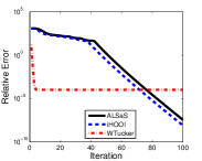
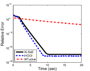
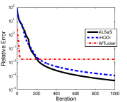
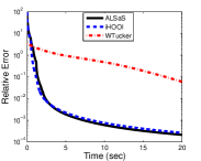
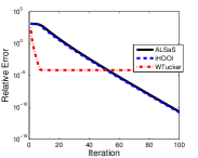
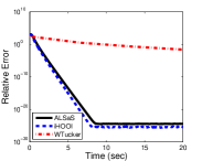
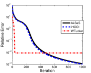
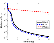
Figure 1: Convergence behavior of ALSaS, iHOOI, and WTucker without using true ranks (first row) and with $r_{n}$’s fixed to true ranks (second row) on $100\times 100\times 100$ (first two columns) and $10\times 10\times 1000$ (last two colums) random tensors.

4.3 Recoverability on factors

In this section, we compare the performance of ALSaS, iHOOI, and WTucker in a different measure. The goal of solving (1) is to get an approximate HOSVD of the underlying tensor $\boldsymbol{{\mathcal{M}}}$, and similarly WTucker is to obtain an approximate Tucker factorization of $\boldsymbol{{\mathcal{M}}}$. For consistent comparison, we normalize the factors given by WTucker in the same way as in (52). Note that the normalization does not change the data fitting. To evaluate the decomposition, we measure the distance of the output factors (after certain rotation) to the original ones. Specifically, suppose that $\boldsymbol{{\mathcal{C}}},\hat{\boldsymbol{{\mathcal{C}}}}\in\mathbb{R}^{r_{1}\times\ldots\times r_{N}}$, and ${\mathbf{A}}_{n},\hat{{\mathbf{A}}}_{n}\in\mathbb{R}^{m_{n}\times r_{n}}$ both have orthonormal columns for all $n$. We let

$${\mathrm{err}}(\boldsymbol{{\mathcal{C}}},{\mathbf{A}};\hat{\boldsymbol{{\mathcal{C}}}},\hat{{\mathbf{A}}})=\frac{\|\boldsymbol{{\mathcal{C}}}\times_{n=1}^{N}{\mathbf{A}}_{n}-\hat{\boldsymbol{{\mathcal{C}}}}\times_{n=1}^{N}\hat{{\mathbf{A}}}_{n}\|_{F}}{\|\boldsymbol{{\mathcal{C}}}\times_{n=1}^{N}{\mathbf{A}}_{n}\|_{F}}+\sum_{n=1}^{N}\frac{\sqrt{r_{n}}-\|{\mathbf{A}}_{n}^{\top}\hat{{\mathbf{A}}}_{n}\|_{F}}{\sqrt{r_{n}}}.$$ (40)

From the following theorem, we have that if ${\mathrm{err}}(\boldsymbol{{\mathcal{C}}},{\mathbf{A}};\hat{\boldsymbol{{\mathcal{C}}}},\hat{{\mathbf{A}}})$ is small, the subspaces spanned by ${\mathbf{A}}_{n}$ and $\hat{{\mathbf{A}}}_{n}$ are close to each other for all $n$, and also after some orthogonal transformation, $\hat{\boldsymbol{{\mathcal{C}}}}$ is close to $\boldsymbol{{\mathcal{C}}}$. It is not difficult to show the theorem, and thus we omit its proof.

Theorem 4.1.

For ${\mathbf{A}}_{n},\hat{{\mathbf{A}}}_{n}\in\mathbb{R}^{m_{n}\times r_{n}}$ with orthonormal columns, it holds that $\|{\mathbf{A}}_{n}^{\top}\hat{{\mathbf{A}}}_{n}\|_{F}\leq\sqrt{r_{n}}$. If the inequality holds with equality, then ${\mathbf{A}}_{n}^{\top}\hat{{\mathbf{A}}}_{n}$ is orthogonal and $\hat{{\mathbf{A}}}_{n}={\mathbf{A}}_{n}{\mathbf{A}}_{n}^{\top}\hat{{\mathbf{A}}}_{n}$. In addition, if $\boldsymbol{{\mathcal{C}}}\times_{n=1}^{N}{\mathbf{A}}_{n}=\hat{\boldsymbol{{\mathcal{C}}}}\times_{n=1}^{N}\hat{{\mathbf{A}}}_{n}$ and $\|{\mathbf{A}}_{n}^{\top}\hat{{\mathbf{A}}}_{n}\|_{F}=\sqrt{r_{n}},\,\forall n$, then $\boldsymbol{{\mathcal{C}}}=\hat{\boldsymbol{{\mathcal{C}}}}\times_{n=1}^{N}({\mathbf{A}}_{n}^{\top}\hat{{\mathbf{A}}}_{n}).$

We test the three algorithms on two random datasets. The first set consists of $50\times 50\times 50$ random tensors and the second one $30\times 30\times 30\times 30$. They are first generated in the same way as that in section 4.2 with ${\hbox{rank}}({\mathbf{M}}_{(n)})=r,\forall n$, and then factor matrix ${\mathbf{A}}_{n}$’s are orthonormalized. We compare the performance of ALSaS, iHOOI, and WTucker on different $r$’s and sample ratios defined as

$$\mathrm{SR}:=\frac{|\Omega|}{\Pi_{i=1}^{N}m_{i}},$$

where $|\Omega|$ denotes the cardinality of $\Omega$. The indices in $\Omega$ are selected uniformly at random. For each pair of $r$ and SR, we generate 30 tensors independently and run the three algorithms with fixed $r_{n}=r,\forall n$ to 2000 iterations or stopping tolerance $10^{-6}$. All three algorithms start from the same random points. Let $(\boldsymbol{{\mathcal{C}}},{\mathbf{A}})$ be the generated factors and $(\hat{\boldsymbol{{\mathcal{C}}}},\hat{{\mathbf{A}}})$ the output of an algorithm. If ${\mathrm{err}}(\boldsymbol{{\mathcal{C}}},{\mathbf{A}};\hat{\boldsymbol{{\mathcal{C}}}},\hat{{\mathbf{A}}})\leq 10^{-2}$, we regard the recovery to be successful. Figure 2 shows the rates of successful recovery by each algorithm. From the figure, we see that iHOOI performs the same as ALSaS in all cases except at $r=21$ and $\mathrm{SR}=30\%$ in the second dataset where the former is slightly better. Both ALSaS and iHOOI perform much better than WTucker in particular for the second dataset.

Figure 2: Rates of successfully recovering factors by ALSaS, iHOOI, and WTucker on $50\times 50\times 50$ (first row) and $30\times 30\times 30\times 30$ (second row) randomly generated tensors for different multilinear ranks and sample ratios.

SR=10%	SR=30%	SR=50%

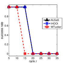
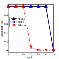
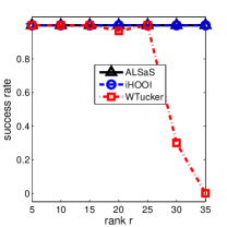
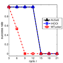
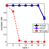
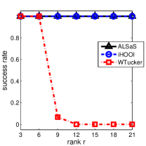
4.4 Application to face recognition

In this subsection, we use the factors obtained from ALSaS, iHOOI, and WTucker for face recognition and compare their prediction accuracies. As in the previous test, we normalize the factors given by WTucker. We use the cropped images in the extended Yale Face Database B [13, 21], which has 38 subjects with each one consisting of 64 face images taken under different illuminations. Each image originally has pixels of $168\times 192$ and is downsampled into $51\times 58$ in our test. We vectorize each downsampled image and form the dataset into a $38\times 64\times 2958$ tensor. Some face images of the first subject are shown in Figure 3.

Figure 3: Selected face images of the first subject in the extended Yale Face Database B corresponding to 16 different illuminations.

We uniformly randomly pick 54 illuminations of images for training and use the remaings for testing. For the training data, we further remove $100(1-\text{SR})$ percent of pixels uniformly at random and then apply the three algorithms to the incomplete training data to get its approximate HOSVD with core size $38\times 54\times r$. Assume the factors of the approximate HOSVD to be $(\hat{\boldsymbol{{\mathcal{C}}}},\hat{{\mathbf{A}}})$. Then $\hat{{\mathbf{A}}}_{3}$ approximately spans the dominant $r$-dimensional subspace of the pixel domain, and $\hat{{\mathbf{B}}}_{3}={\mathbf{unfold}}_{3}(\hat{\boldsymbol{{\mathcal{C}}}}\times_{1}\hat{{\mathbf{A}}}_{1}\times\hat{{\mathbf{A}}}_{2})$ contains the coefficients of images in the training set. For each image ${\mathbf{x}}$ in the testing set, we compare the coefficient vector $\hat{{\mathbf{A}}}_{3}^{\top}{\mathbf{x}}$ to each column of $\hat{{\mathbf{B}}}_{3}$ and classify ${\mathbf{x}}$ to be the subject corresponding to the closest column. We vary SR among $\{10\%,30\%,50\%,70\%\}$ and $r$ among $\{50,75,100\}$. For each pair of SR and $r$, we repeat the whole process (i.e., randomly choosing training dataset, removing pixels, obtaining approximate HOSVD, and performing classification) 3 times independently and take the average of the classification accuracies (i.e., the ratio of the number of correctly recognized face images over the total testing images) and running time. We compare the tensor face recognition methods to EigenFace, a popular matrix face recognition method, which reshapes each face image into a vector, forms a matrix with each column being a reshaped face image, and then performs eigendecomposition to find a basis for recognition. Table 1 shows the average results of each algorithm and also accuracies by EigenFace using incomplete training data as a baseline. From the table, we see that all the three algorithms give similar classification accuracies since they solve similar models, and iHOOI performs slightly better than ALSaS and WTucker in most cases. In addition, ALSaS is the fastest while WTucker costs much more time than that by ALSaS and also iHOOI in every case. Note that larger $r$ gives higher accuracies except at $\text{SR}=10\%$ because too few observations and large $r$ cause overfitting problem.

Table 1: Average classification accuracies (in percentage) and running time (in second) of ALSaS, iHOOI, and WTucker on the extended Yale Database B for face recognition. The numbers in the parenthesis denote the corresponding average running time. The highest accuracies for each pair of SR and $r$ are highlighted in bold.

	$r=50$				$r=75$				$r=100$
SR	ALSaS	iHOOI	WTucker	EigenFace	ALSaS	iHOOI	WTucker	EigenFace	ALSaS	iHOOI	WTucker	EigenFace
10%	64.12(515)	66.31(1606)	63.33(4874)	4.65	62.46(507)	65.88(1506)	57.28(6366)	5.35	59.47(497)	63.51(1396)	55.43(5315)	7.46
30%	73.42(144)	73.60(197)	73.95(2566)	11.84	78.42(166)	78.86(246)	78.25(2833)	17.98	80.70(207)	80.79(401)	80.35(3164)	21.32
50%	71.67(120)	72.02(164)	72.37(2171)	21.14	77.98(136)	77.98(180)	77.72(2331)	31.32	81.05(166)	80.79(207)	81.05(2457)	37.98
70%	76.84(108)	76.93(157)	75.96(1894)	57.72	81.49(131)	81.40(171)	81.23(2038)	65.44	83.60(155)	83.42(200)	83.42(2111)	69.30

4.5 Low-rank tensor completion

Upon recovering factors $\boldsymbol{{\mathcal{C}}}$ and ${\mathbf{A}}$, one can easily estimate missing entries of the underlying tensor $\boldsymbol{{\mathcal{M}}}$. When $\boldsymbol{{\mathcal{M}}}$ has low multilinear rank, it can be exactly reconstructed under certain conditions (see [16, 48] for example). In this subsection, we test ALSaS and iHOOI on reconstructing (approximately) low-multilinear-rank tensors and compare them to WTucker and two other state-of-the-art methods: TMac [45] and geomCG [19]. We choose TMac and geomCG for comparison because their codes are publicly available and also they have been shown superior over several other tensor-completion methods including FaLRTC [23] and SquareDeal [27]. TMac is an alternating least squares method for solving the so-called parallel matrix factorization model:

$$\begin{array}[]{l}\underset{{\mathbf{X}},{\mathbf{Y}},\boldsymbol{{\mathcal{Z}}}}{\min}\sum_{n=1}^{N}\alpha_{n}\|{\mathbf{X}}_{n}{\mathbf{Y}}_{n}^{\top}-{\mathbf{unfold}}_{n}(\boldsymbol{{\mathcal{Z}}})\|_{F}^{2},\\[2.84544pt] \mbox{ s.t. }{\mathcal{P}}_{\Omega}(\boldsymbol{{\mathcal{Z}}})={\mathcal{P}}_{\Omega}(\boldsymbol{{\mathcal{M}}}),\,{\mathbf{X}}_{n}\in\mathbb{R}^{m_{n}\times r_{n}},{\mathbf{Y}}_{n}\in\mathbb{R}^{(\Pi_{i\neq n}m_{i})\times r_{n}},\forall n,\end{array}$$ (41)

and geomCG is a Riemannian conjugate gradient method for

$$\min_{\boldsymbol{{\mathcal{X}}}}\frac{1}{2}\|{\mathcal{P}}_{\Omega}(\boldsymbol{{\mathcal{X}}})-{\mathcal{P}}_{\Omega}(\boldsymbol{{\mathcal{M}}})\|_{F}^{2},\mbox{ s.t. }{\hbox{rank}}\big{(}{\mathbf{unfold}}_{n}(\boldsymbol{{\mathcal{X}}})\big{)}=r_{n},\,n=1,\ldots,N.$$ (42)

In (41), $\sum_{n}\alpha_{n}=1$, and $\alpha_{n}$ acts as a weight on the $n$-th mode fitting and can be adaptively updated. Usually, better low-rankness property leads to better data fitting, and larger $\alpha_{n}$ is put. Since all tensors tested in this subsection are balanced and have similar low-rankness along each mode, we simply fix $\alpha_{n}=\frac{1}{N},\,\forall n$. Both (41) and (42) require estimation on $r_{n}$’s, which can be either fixed or adaptively adjusted in a similar way as that for ALSaS and iHOOI. First, we compare the recoverability of the five methods on randomly generated low-multilinear-rank tensors. Then, we test their accuracies and efficiency on reconstructing a 3D MRI image.

Phase transition plots

A phase transition plot uses greyscale colors to depict how likely a certain kind of low-multilinear-rank tensors can be recovered by an algorithm for a range of different ranks and sample ratios. Phase transition plots are important means to compare the performance of different tensor recovery methods.

We use two random datasets in the test. Each tensor in both sets is $50\times 50\times 50$ and has the form of $\boldsymbol{{\mathcal{M}}}=\boldsymbol{{\mathcal{C}}}\times_{1}{\mathbf{A}}_{1}\times_{2}{\mathbf{A}}_{2}\times_{3}{\mathbf{A}}_{3}$. In the first dataset, entries of $\boldsymbol{{\mathcal{C}}}$ and ${\mathbf{A}}_{n}$’s follow standard normal distribution: $\boldsymbol{{\mathcal{C}}}$ is generated by MATLAB command randn(r,r,r) and ${\mathbf{A}}_{n}$ by randn(50,r) for $n=1,2,3$. In the second dataset, entries of $\boldsymbol{{\mathcal{C}}}$ follow uniform distribution, and ${\mathbf{A}}_{n}$’s have power-law decaying singular values: $\boldsymbol{{\mathcal{C}}}$ is generated by command rand(r,r,r) and ${\mathbf{A}}_{n}$ by orth(randn(50,r))*diag([1:r].^(-0.5)) for $n=1,2,3$. Usually, the tensors in the second dataset is more difficult to recover than those in the first one. For both datasets, we generate $\Omega$ uniformly at random, and we vary $r$ from 5 to 35 with increment 3 and SR from 10% to 90% with increment 5%. We regard the recovery $\boldsymbol{{\mathcal{M}}}^{rec}$ to be successful, if

$$\mathrm{relerr}(\boldsymbol{{\mathcal{M}}}^{rec}):=\frac{\|\boldsymbol{{\mathcal{M}}}^{rec}-\boldsymbol{{\mathcal{M}}}\|_{F}}{\|\boldsymbol{{\mathcal{M}}}\|_{F}}\leq 10^{-2}.$$

We apply rank-increasing and rank-fixing strategies to ALSaS, iHOOI, TMac and geomCG, and we append “-inc” and “-fix” respectively after the name of each algorithm to specify which strategy is applied. The rank-increasing strategy initializes $r_{n}=1$ for all four algorithms and sets $r_{n}^{\max}=50,\forall n$ for the former three and $r_{n}^{\max}=r,\forall n$ for geomCG, and the rank-fixing strategy fixes $r_{n}=r,\,n=1,2,3$. We test WTucker with true ranks (WTucker-true) by fixing $r_{n}=r,\forall n$ and also rank over estimation (WTucker-over) by fixing $r_{n}=r+10,\forall n$. All the algorithms are provided with the same random starting points. For each pair of $r$ and SR, we run all the algorithms on 50 independently generated low-multilinear-rank tensors. To save testing time, we simply regard that if an algorithm succeeds 50 times at some pair of $r$ and SR, it will alway succeeds at this $r$ for larger SR’s, and if it fails 50 times at some pair of $r$ and SR, it will never succeed at this SR for larger $r$’s. Figure 4 depicts the phase transition plot of each method on the Gaussian randomly generated tensors and Figure 5 on random tensors with power-law decaying singular values. From the figures, we see that ALSaS and iHOOI performs comparably well to TMac with both rank-increasing and rank-fixing strategies and also to geomCG with rank-increasing strategy. In addition, even without knowing the true ranks, ALSaS and iHOOI by adaptively increasing rank estimates can perform as well as those by assuming true ranks. Both ALSaS and iHOOI successfully recover more low-multilinear-rank tensors than WTucker, and geomCG with rank-fixing strategy.

Figure 4: Phase transition plots of different methods on 3-way random tensors whose factors have Gaussian random entries. ALSaS and iHOOI are the proposed methods; TMac [45] solves (41); geomCG [19] solves (42); WTucker [8] solves a model similar to (1) without orthogonality constraint on ${\mathbf{A}}_{n}$’s.

ALSaS-inc	iHOOI-inc	TMac-inc	geomCG-inc	WTucker-over
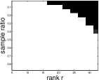
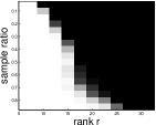
ALSaS-fix	iHOOI-fix	TMac-fix	geomCG-fix	WTucker-true

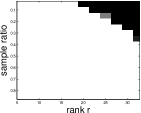
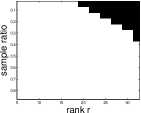
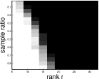
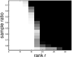
Figure 5: Phase transition plots of different methods on 3-way random tensors whose factors have power-law decaying singular values. ALSaS and iHOOI are the proposed methods; TMac [45] solves (41); geomCG [19] solves (42); WTucker [8] solves a model similar to (1) without orthogonality constraint on ${\mathbf{A}}_{n}$’s.

ALSaS-inc	iHOOI-inc	TMac-inc	geomCG-inc	WTucker-over
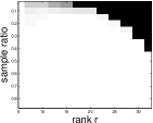
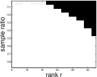
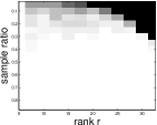
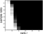
ALSaS-fix	iHOOI-fix	TMac-fix	geomCG-fix	WTucker-true

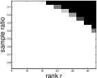
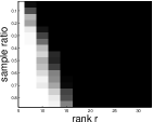
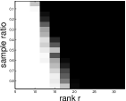
Application to MRI image reconstruction

We compare the performance of the above five algorithms on reconstructing a 3D brain MRI image, which has been used in [23, 45] for low-rank tensor completion test. The MRI dataset has 181 images of resolution $217\times 181$. We form it into a $181\times 217\times 181$ tensor, and Figure 6 plots its scaled singular values of each mode matricization. From the figure, we see that the dataset has very good multilinear low-rankness property, and it can be well approximated by a rank-$(50,50,50)$ tensor. Hence, we set $r_{n}^{\max}=50$ and initialize $r_{n}=1,n=1,2,3$ for ALSaS, iHOOI, TMac, and geomCG and fix $r_{n}=50,n=1,2,3$ for WTucker. Figure 7 depicts three slices of the original and 95% masked data and corresponding reconstructed ones by ALSaS and iHOOI, and Table 2 gives the average relative reconstruction errors and running time of 3 independent trials by the five algorithms from 5% and 10% entries sampled uniformly at random. From the table, we see that ALSaS, iHOOI, TMac, and geomCG can all give highly accurate reconstructions while WTucker achieves a relatively lower accuracy. In addition, geomCG and WTucker takes much more time than the other three and iHOOI is the fastest one among the compared methods.

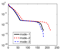
Figure 6: Scaled singular values of each mode matricization of a $181\times 217\times 181$ brain MRI image.

Figure 7: Brain MRI images: three original slices, the corresponding slices with 95% pixels missing, and the reconstructed slices by ALSaS and iHOOI.

Original	95% masked	ALSaS	iHOOI

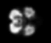
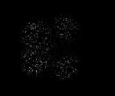
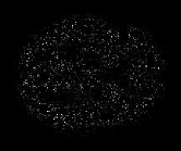
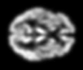
Table 2: Average relative reconstruction errors (abbreviated as relerr) and running time (in second) of ALSaS, iHOOI, TMac, geomCG, and WTucker from 5% and 10% uniformly randomly sampled entries of a $181\times 217\times 181$ MRI dataset. The most accurate solutions are highlighted in bold.

	ALSaS		iHOOI		TMac		geomCG		WTucker
SR	relerr	time	relerr	time	relerr	time	relerr	time	relerr	time
5%	2.04e-4	580	1.97e-4	377	2.94e-4	711	1.80e-4	5055	1.45e-2	4580
10%	2.85e-5	357	2.77e-5	310	3.36e-5	319	4.36e-5	12243	9.78e-3	5652

5 Conclusions

We have formulated an incomplete higher-order singular value decomposition (HOSVD) problem and also presented one algorithm, called iHOOI, for solving the problem based on block coordinate update. Under boundedness assumption on the iterates, we have shown the global convergence of iHOOI in terms of a first-order optimality condition if there is a positive gap between the $r_{n}$-th and $(r_{n}+1)$-th largest singular values of intermediate points. Hence, for the first time, we have given global convergence of the popular higher-order orthogonality iteration (HOOI) method by regarding it as a special case of iHOOI. In addition, we have tested the efficiency and reliability of the proposed method on obtaining dominant factors of underlying tensors and also reconstructing low-multilinear-rank tensors, on both of which we have demonstrated that it can outperform state-of-the-art methods.

Appendix A Alternating least squares

We present another algorithm for finding an approximate higher-order singular value decomposition of an given tensor $\boldsymbol{{\mathcal{M}}}$ from its partial entries. This algorithm is based on the alternating least squares method for solving (8).

Note that in (8), $f$ is convex with respect to each block variable among $\boldsymbol{{\mathcal{C}}},{\mathbf{A}}_{1},\ldots,{\mathbf{A}}_{N}$ and $\boldsymbol{{\mathcal{X}}}$ while keeping the others fixed. In addition, we have $\boldsymbol{{\mathcal{C}}}\times_{i=1}^{N}({\mathbf{A}}_{i}{\mathbf{R}}_{i})=(\boldsymbol{{\mathcal{C}}}\times_{i=1}^{N}{\mathbf{R}}_{i})\times_{i=1}^{N}{\mathbf{A}}_{i}$ from (3). Hence, we propose to solve (8) by first cyclically updating $\boldsymbol{{\mathcal{C}}},{\mathbf{A}}_{1},\ldots,{\mathbf{A}}_{N}$ and $\boldsymbol{{\mathcal{X}}}$ without orthogonality constraint and then normalizing ${\mathbf{A}}_{n}$’s at the end of each cycle. Specifically, let $(\hat{\boldsymbol{{\mathcal{C}}}},\hat{{\mathbf{A}}},\hat{\boldsymbol{{\mathcal{X}}}})$ be the current value of the variables. We renew $({\boldsymbol{{\mathcal{C}}}},{{\mathbf{A}}})$ to $(\tilde{\boldsymbol{{\mathcal{C}}}},\tilde{{\mathbf{A}}})$ by first performing the updates

$$\boldsymbol{\mathcal{C}}^{mid} =\operatorname*{arg\,min}_{\boldsymbol{\mathcal{C}}}f(\boldsymbol{\mathcal{C}},\hat{\mathbf{A}},\hat{\boldsymbol{\mathcal{X}}}),$$ (43a)

$$\mathbf{A}_{n}^{mid} =\operatorname*{arg\,min}_{\mathbf{A}_{n}}f(\boldsymbol{\mathcal{C}}^{mid},\mathbf{A}_{<n}^{mid},\mathbf{A}_{n},\hat{\mathbf{A}}_{>n},\hat{\boldsymbol{\mathcal{X}}}),\ n=1,\ldots,N,$$ (43b)

Assuming the economy QR decomposition of ${\mathbf{A}}_{n}^{mid}$ to be ${\mathbf{A}}_{n}^{mid}={\mathbf{Q}}_{n}{\mathbf{R}}_{n},\,n=1,\ldots,N$, we then let

$$\tilde{\boldsymbol{{\mathcal{C}}}}=\boldsymbol{{\mathcal{C}}}^{mid}\times_{i=1}^{N}{\mathbf{R}}_{i},\quad\tilde{{\mathbf{A}}}_{n}={\mathbf{Q}}_{n},\,n=1,\ldots,N.$$

We renew ${\boldsymbol{{\mathcal{X}}}}$ to $\tilde{\boldsymbol{{\mathcal{X}}}}$ by

$$\tilde{\boldsymbol{\mathcal{X}}}=\operatorname*{arg\,min}_{\mathcal{P}_{\Omega}(\boldsymbol{\mathcal{X}})=\mathcal{P}_{\Omega}(\boldsymbol{\mathcal{M}})}f(\tilde{\boldsymbol{\mathcal{C}}},\tilde{\mathbf{A}},\boldsymbol{\mathcal{X}}),$$ (44)

which can be explicitly written as

$$\tilde{\boldsymbol{\mathcal{X}}}=\mathcal{P}_{\Omega^{c}}(\tilde{\boldsymbol{\mathcal{C}}}\times_{1}\tilde{\mathbf{A}}_{1}\ldots\times_{N}\tilde{\mathbf{A}}_{N})+\mathcal{P}_{\Omega}(\boldsymbol{\mathcal{M}}).$$ (45)

$\boldsymbol{{\mathcal{C}}}$- and ${\mathbf{A}}$-subproblems

According to (5), the problem in (43a) can be written as

$$\boldsymbol{\mathcal{C}}^{mid}=\operatorname*{arg\,min}_{\boldsymbol{\mathcal{C}}}\frac{1}{2}\big{\|}\big{(}\otimes_{n=N}^{1}\hat{\mathbf{A}}_{n}\big{)}{\mathrm{vec}}(\boldsymbol{\mathcal{C}})-{\mathrm{vec}}(\hat{\boldsymbol{\mathcal{X}}})\big{\|}_{2}^{2},$$ (46)

the solution of which can be written as

$${\mathrm{vec}}(\boldsymbol{\mathcal{C}}^{mid})=\left(\big{(}\otimes_{n=N}^{1}\hat{\mathbf{A}}_{n}\big{)}^{\top}\big{(}\otimes_{n=N}^{1}\hat{\mathbf{A}}_{n}\big{)}\right)^{\dagger}\left(\big{(}\otimes_{n=N}^{1}\hat{\mathbf{A}}_{n}\big{)}^{\top}{\mathrm{vec}}(\hat{\boldsymbol{\mathcal{X}}})\right).$$

Using (5) and (7) and noticing $\hat{{\mathbf{A}}}_{n}^{\top}\hat{{\mathbf{A}}}_{n}={\mathbf{I}},\,\forall n$, we have

$$\boldsymbol{\mathcal{C}}^{mid}=\hat{\boldsymbol{\mathcal{X}}}\times_{1}\hat{\mathbf{A}}_{1}^{\top}\ldots\times_{N}\hat{\mathbf{A}}_{N}^{\top}.$$ (47)

Let $\hat{\mathbf{B}}_{n}={\mathbf{unfold}}_{n}(\mathbf{C}^{mid}\times_{i=1}^{n-1}\mathbf{A}_{i}^{mid}\times_{i=n+1}^{N}\hat{\mathbf{A}}_{i}).$ Then according to (4), each problem in (43b) can be written as

$$\mathbf{A}_{n}^{mid}=\operatorname*{arg\,min}_{\mathbf{A}_{n}}\frac{1}{2}\big{\|}\mathbf{A}_{n}\hat{\mathbf{B}}_{n}-\hat{\mathbf{X}}_{(n)}\big{\|}_{F}^{2},$$ (48)

whose solution can be explicitly written as

$$\mathbf{A}_{n}^{mid}=\hat{\mathbf{X}}_{(n)}(\hat{\mathbf{B}}_{n})^{\top}\big{(}\hat{\mathbf{B}}_{n}\hat{\mathbf{B}}_{n}^{\top}\big{)}^{\dagger}.$$ (49)

Summarizing the above discussion, we have the pseudocode of the proposed method in Algorithm 2.

Algorithm 2 Alternating Least Squares for HOSVD with missing values (ALSaS)

1:  Input: index set $\Omega$, observed entries $\mathcal{P}_{\Omega}(\boldsymbol{\mathcal{M}})$, and initial point $(\boldsymbol{\mathcal{C}}^{0},\mathbf{A}^{0},\boldsymbol{\mathcal{X}}^{0})$ with $({\mathbf{A}}_{i}^{0})^{\top}{\mathbf{A}}_{i}^{0}={\mathbf{I}},\forall i$ and $\mathcal{P}_{\Omega}(\boldsymbol{\mathcal{X}}^{0})=\mathcal{P}_{\Omega}(\boldsymbol{\mathcal{M}})$.

2:  for $k=0,1,\ldots$ do

3:     Update $\boldsymbol{{\mathcal{C}}}$ by

$$\boldsymbol{{\mathcal{C}}}^{k+\frac{1}{2}}=\boldsymbol{\mathcal{X}}^{k}\times_{i=1}^{N}(\mathbf{A}_{i}^{k})^{\top}.$$ (50)

4:     for $n=1,\ldots,N$ do

5:        Update ${\mathbf{A}}_{n}$ by

$${\mathbf{A}}_{n}^{k+\frac{1}{2}}=\boldsymbol{{\mathcal{X}}}_{(n)}^{k}({\mathbf{B}}_{n}^{k})^{\top}({\mathbf{B}}_{n}^{k}({\mathbf{B}}_{n}^{k})^{\top})^{\dagger},$$

where

$${\mathbf{B}}_{n}^{k}={\mathbf{unfold}}_{n}\big{(}\boldsymbol{{\mathcal{C}}}^{k+\frac{1}{2}}\times_{i=1}^{n-1}{\mathbf{A}}_{i}^{k+\frac{1}{2}}\times_{i=n+1}^{N}{\mathbf{A}}_{i}^{k}\big{)}.$$ (51)

6:     end for

7:     Let the economy QR decomposition of ${\mathbf{A}}_{n}^{k+\frac{1}{2}}$ be ${\mathbf{Q}}_{n}^{k}{\mathbf{R}}_{n}^{k}$ and do the normalization

$$\boldsymbol{{\mathcal{C}}}^{k+1}=\boldsymbol{{\mathcal{C}}}^{k+\frac{1}{2}}\times_{i=1}^{N}{\mathbf{R}}_{i}^{k},\quad{\mathbf{A}}_{n}^{k+1}={\mathbf{Q}}_{n}^{k},\,n=1,\ldots,N.$$ (52)

8:     Update $\boldsymbol{{\mathcal{X}}}$ by

$$\boldsymbol{\mathcal{X}}^{k+1}=\mathcal{P}_{\Omega^{c}}(\boldsymbol{\mathcal{C}}^{k+1}\times_{i=1}^{N}\mathbf{A}_{i}^{k+1})+\mathcal{P}_{\Omega}(\boldsymbol{\mathcal{M}}).$$ (53)

9:     if stopping criterion is satisfied then

10:        Return $(\boldsymbol{\mathcal{C}}^{k+1},\mathbf{A}^{k+1},\boldsymbol{\mathcal{X}}^{k+1})$.

11:     end if

12:  end for

Following the convergence analysis of [45], it is not difficult to show the global convergence of Algorithm 2, and we summarize the result as follows with no proof.

Theorem A.1 (Global convergence of Algorithm 2).

Let $\{(\boldsymbol{{\mathcal{C}}}^{k},{\mathbf{A}}^{k},\boldsymbol{{\mathcal{X}}}^{k})\}_{k=1}^{\infty}$ be the sequence generated from Algorithm 2. Also, let $\boldsymbol{{\mathcal{Y}}}^{k}={\mathcal{P}}_{\Omega}(\boldsymbol{{\mathcal{C}}}^{k}\times_{i=1}^{N}{\mathbf{A}}_{i}^{k})-{\mathcal{P}}_{\Omega}(\boldsymbol{{\mathcal{M}}})$ and $\boldsymbol{\Lambda}^{k}=\mathbf{0}$ for all $k$. Then any finite limit point of $\{(\boldsymbol{{\mathcal{C}}}^{k},{\mathbf{A}}^{k},\boldsymbol{{\mathcal{X}}}^{k},\boldsymbol{\Lambda}^{k},\boldsymbol{{\mathcal{Y}}}^{k})\}_{k=1}^{\infty}$ satisfies the first-order optimality conditions of (8). Furthermore, if $\{{\mathcal{P}}_{\Omega^{c}}(\boldsymbol{{\mathcal{X}}}^{k})\}_{k=1}^{\infty}$ is bounded, then

$$\lim_{k\to\infty}\nabla{\mathcal{L}}_{f}(\boldsymbol{{\mathcal{C}}}^{k},{\mathbf{A}}^{k},\boldsymbol{{\mathcal{X}}}^{k},\boldsymbol{\Lambda}^{k},\boldsymbol{{\mathcal{Y}}}^{k})=\mathbf{0}.$$ (54)

Appendix B Proof of (14)

Let ${\mathbf{D}}_{1},{\mathbf{D}}_{2}$ be diagonal matrices such that $\mathrm{vec}({\mathcal{P}}_{\Omega}(\boldsymbol{{\mathcal{X}}}))={\mathbf{D}}_{1}\mathrm{vec}(\boldsymbol{{\mathcal{X}}})$ and $\mathrm{vec}({\mathcal{P}}_{\Omega^{c}}(\boldsymbol{{\mathcal{X}}}))={\mathbf{D}}_{2}\mathrm{vec}(\boldsymbol{{\mathcal{X}}})$ respectively. Then from (5), it follows that

$$h(\boldsymbol{{\mathcal{X}}};\tilde{{\mathbf{A}}})=\frac{1}{2}\big{\|}{\mathbf{D}}_{2}\mathrm{vec}(\boldsymbol{{\mathcal{X}}})\big{\|}^{2}-\frac{1}{2}\big{\|}(\otimes_{i=N}^{1}\tilde{{\mathbf{A}}}_{i}^{\top})({\mathbf{D}}_{2}\mathrm{vec}(\boldsymbol{{\mathcal{X}}})+{\mathbf{D}}_{1}\mathrm{vec}(\boldsymbol{{\mathcal{M}}}))\big{\|}^{2}.$$

Hence,

$${\mathrm{vec}}\big{(}\nabla_{\boldsymbol{{\mathcal{X}}}}h(\hat{\boldsymbol{{\mathcal{X}}}};\tilde{{\mathbf{A}}})\big{)}= \,{\mathbf{D}}_{2}^{\top}{\mathbf{D}}_{2}{\mathrm{vec}}(\hat{\boldsymbol{{\mathcal{X}}}})-{\mathbf{D}}_{2}^{\top}(\otimes_{i=N}^{1}\tilde{{\mathbf{A}}}_{i}^{\top})^{\top}(\otimes_{i=N}^{1}\tilde{{\mathbf{A}}}_{i}^{\top})({\mathbf{D}}_{2}\mathrm{vec}(\hat{\boldsymbol{{\mathcal{X}}}})+{\mathbf{D}}_{1}\mathrm{vec}(\boldsymbol{{\mathcal{M}}}))$$

$$= \,{\mathbf{D}}_{2}{\mathrm{vec}}(\hat{\boldsymbol{{\mathcal{X}}}})-{\mathbf{D}}_{2}(\otimes_{i=N}^{1}\tilde{{\mathbf{A}}}_{i}\tilde{{\mathbf{A}}}_{i}^{\top})({\mathbf{D}}_{2}\mathrm{vec}(\hat{\boldsymbol{{\mathcal{X}}}})+{\mathbf{D}}_{1}\mathrm{vec}(\boldsymbol{{\mathcal{M}}}))$$

$$= \,{\mathbf{D}}_{2}{\mathrm{vec}}(\hat{\boldsymbol{{\mathcal{X}}}})-{\mathbf{D}}_{2}(\otimes_{i=N}^{1}\tilde{{\mathbf{A}}}_{i}\tilde{{\mathbf{A}}}_{i}^{\top})\mathrm{vec}(\hat{\boldsymbol{{\mathcal{X}}}})\qquad(\text{because }{\mathcal{P}}_{\Omega}(\hat{\boldsymbol{{\mathcal{X}}}})={\mathcal{P}}_{\Omega}(\boldsymbol{{\mathcal{M}}})).$$

Using (5), we have

$$\nabla_{\boldsymbol{{\mathcal{X}}}}h(\hat{\boldsymbol{{\mathcal{X}}}};\tilde{{\mathbf{A}}})={\mathcal{P}}_{\Omega^{c}}(\hat{\boldsymbol{{\mathcal{X}}}})-{\mathcal{P}}_{\Omega^{c}}(\hat{\boldsymbol{{\mathcal{X}}}}\times_{i=1}^{N}\tilde{{\mathbf{A}}}_{i}\tilde{{\mathbf{A}}}_{i}^{\top}),$$

which completes the proof.

References

- [1] E. Acar, D. M. Dunlavy, T. G. Kolda, and M. Mørup, Scalable tensor factorizations with missing data., in Proceedings of the SIAM International Conference on Data Mining, (2010), pp. 701–712.
- [2] A. Beck and M. Teboulle, A fast iterative shrinkage-thresholding algorithm for linear inverse problems, SIAM Journal on Imaging Sciences, 2 (2009), pp. 183–202.
- [3] D. P. Bertsekas, Nonlinear Programming, Athena Scientific, September 1999.
- [4] A. M. Buchanan and A. W. Fitzgibbon, Damped newton algorithms for matrix factorization with missing data, in IEEE Computer Society Conference on Computer Vision and Pattern Recognition, 2 (2005), pp. 316–322.
- [5] Y. Chen, C. Hsu, and H. Liao, Simultaneous tensor decomposition and completion using factor priors, (2013).
- [6] L. De Lathauwer, B. De Moor, and J. Vandewalle, A multilinear singular value decomposition, SIAM Journal on Matrix Analysis and Applications, 21 (2000), pp. 1253–1278.
- [7] , On the best rank-1 and rank- approximation of higher-order tensors, SIAM Journal on Matrix Analysis and Applications, 21 (2000), pp. 1324–1342.
- [8] M. Filipović and A. Jukić, Tucker factorization with missing data with application to low-n-rank tensor completion, Multidimensional Systems and Signal Processing, (2013), pp. 1–16.
- [9] K. R. Gabriel and S. Zamir, Lower rank approximation of matrices by least squares with any choice of weights, Technometrics, 21 (1979), pp. 489–498.
- [10] S. Gandy, B. Recht, and I. Yamada, Tensor completion and low--rank tensor recovery via convex optimization, Inverse Problems, 27 (2011), pp. 1–19.
- [11] X. Geng and K. Smith-Miles, Facial age estimation by multilinear subspace analysis, in IEEE International Conference on Acoustics, Speech and Signal Processing (ICASSP), (2009), pp. 865–868.
- [12] X. Geng, K. Smith-Miles, Z.-H. Zhou, and L. Wang, Face image modeling by multilinear subspace analysis with missing values, IEEE Transactions on Systems, Man, and Cybernetics, Part B: Cybernetics, 41 (2011), pp. 881–892.
- [13] A. S. Georghiades, P. N. Belhumeur, and D. Kriegman, From few to many: Illumination cone models for face recognition under variable lighting and pose, IEEE Transactions on Pattern Analysis and Machine Intelligence, 23 (2001), pp. 643–660.
- [14] G. H. Golub and C. F. Van Loan, Matrix computations, Johns Hopkins Studies in the Mathematical Sciences, Johns Hopkins University Press, Baltimore, MD, third ed., 1996.
- [15] R. Horn and C. Johnson, Topics in matrix analysis, Cambridge Univ. Press Cambridge etc, 1991.
- [16] B. Huang, C. Mu, D. Goldfarb, and J. Wright, Provable low-rank tensor recovery, Pacific Journal of Optimization, 11 (2015), pp. 339–364.
- [17] T. Kolda and B. Bader, Tensor decompositions and applications, SIAM review, 51 (2009), pp. 455–500.
- [18] N. Kreimer and M. D. Sacchi, A tensor higher-order singular value decomposition for prestack seismic data noise reduction and interpolation, Geophysics, 77 (2012), pp. 113–122.
- [19] D. Kressner, M. Steinlechner, and B. Vandereycken, Low-rank tensor completion by riemannian optimization, BIT Numerical Mathematics, (2013), pp. 1–22.
- [20] M. Kurucz, A. A. Benczúr, and K. Csalogány, Methods for large scale svd with missing values, in Proceedings of KDD Cup and Workshop, vol. 12, Citeseer, 2007, pp. 31–38.
- [21] K.-C. Lee, J. Ho, and D. Kriegman, Acquiring linear subspaces for face recognition under variable lighting, IEEE Transactions on Pattern Analysis and Machine Intelligence, 27 (2005), pp. 684–698.
- [22] Q. Ling, Y. Xu, W. Yin, and Z. Wen, Decentralized low-rank matrix completion, in IEEE International Conference on Acoustics, Speech and Signal Processing (ICASSP), (2012), pp. 2925–2928.
- [23] J. Liu, P. Musialski, P. Wonka, and J. Ye, Tensor completion for estimating missing values in visual data, IEEE Transactions on Pattern Analysis and Machine Intelligence, (2013), pp. 208–220.
- [24] Y. Liu, F. Shang, H. Cheng, J. Cheng, and H. Tong, Factor matrix trace norm minimization for low-rank tensor completion, Proceedings of the 2014 SIAM International Conference on Data Mining, (2014).
- [25] L. Mirsky, A trace inequality of John von Neumann, Monatshefte für mathematik, 79 (1975), pp. 303–306.
- [26] M. Mørup, L. Hansen, and S. Arnfred, Algorithms for sparse nonnegative Tucker decompositions, Neural computation, 20 (2008), pp. 2112–2131.
- [27] C. Mu, B. Huang, J. Wright, and D. Goldfarb, Square deal: Lower bounds and improved relaxations for tensor recovery, arXiv preprint arXiv:1307.5870, (2013).
- [28] L. Omberg, G. H. Golub, and O. Alter, A tensor higher-order singular value decomposition for integrative analysis of dna microarray data from different studies, Proceedings of the National Academy of Sciences, 104 (2007), pp. 18371–18376.
- [29] P. Paatero, A weighted non-negative least squares algorithm for three-way ‘parafac’factor analysis, Chemometrics and Intelligent Laboratory Systems, 38 (1997), pp. 223–242.
- [30] Z. Peng, T. Wu, Y. Xu, M. Yan, and W. Yin, Coordinate Friendly Structures, Algorithms and Applications, Annals of Mathematical Sciences and Applications, 1 (2016), pp. 57–119.
- [31] A. Phan, P. Tichavsky, and A. Cichocki, Damped gauss-newton algorithm for nonnegative tucker decomposition, in IEEE Statistical Signal Processing Workshop (SSP), (2011), pp. 665–668.
- [32] B. Romera-Paredes and M. Pontil, A new convex relaxation for tensor completion, arXiv preprint arXiv:1307.4653, (2013).
- [33] A. Ruhe, Numerical computation of principal components when several observations are missing, University of Umea, Institute of Mathematics and Statistics Report, (1974).
- [34] B. Savas and L. Eldén, Handwritten digit classification using higher order singular value decomposition, Pattern recognition, 40 (2007), pp. 993–1003.
- [35] L. Sorber, M. Van Barel, and L. De Lathauwer, Structured data fusion, ESAT-STADIUS, KU Leuven, Belgium, Tech. Rep, (2013), pp. 13–177.
- [36] N. Srebro and T. Jaakkola, Weighted low-rank approximations, in Machine Learning International Workshop, 20 (2003), pp. 720–727.
- [37] J.-T. Sun, H.-J. Zeng, H. Liu, Y. Lu, and Z. Chen, Cubesvd: a novel approach to personalized web search, in Proceedings of the 14th international conference on World Wide Web, ACM, 2005, pp. 382–390.
- [38] G. Tomasi and R. Bro, Parafac and missing values, Chemometrics and Intelligent Laboratory Systems, 75 (2005), pp. 163–180.
- [39] A. Uschmajew, A new convergence proof for the high-order power method and generalizations, Arxiv preprint arXiv:1407.4586, (2014).
- [40] M. A. O. Vasilescu, Human motion signatures: Analysis, synthesis, recognition, in Proceedings of IEEE 16th International Conference on Pattern Recognition, 3 (2002), pp. 456–460.
- [41] M. A. O. Vasilescu and D. Terzopoulos, Multilinear image analysis for facial recognition, in IEEE Computer Society International Conference on Pattern Recognition, 2 (2002), pp. 20511–20511.
- [42] B. Walczak and D. Massart, Dealing with missing data: Part i, Chemometrics and Intelligent Laboratory Systems, 58 (2001), pp. 15–27.
- [43] Z. Wen, W. Yin, and Y. Zhang, Solving a low-rank factorization model for matrix completion by a nonlinear successive over-relaxation algorithm, Mathematical Programming Computation, (2012), pp. 1–29.
- [44] Y. Xu, Alternating proximal gradient method for sparse nonnegative tucker decomposition, Mathematical Programming Computation, 7 (2015), pp. 39–70.
- [45] Y. Xu, R. Hao, W. Yin, and Z. Su, Parallel matrix factorization for low-rank tensor completion, Inverse Problems and Imaging, 9 (2015), pp. 601–624.
- [46] Y. Xu and W. Yin, A block coordinate descent method for regularized multiconvex optimization with applications to nonnegative tensor factorization and completion, SIAM Journal on Imaging Sciences, 6 (2013), pp. 1758–1789.
- [47] Y. Xu, W. Yin, Z. Wen, and Y. Zhang, An alternating direction algorithm for matrix completion with nonnegative factors, Frontiers of Mathematics in China, 7 (2012), pp. 365–384.
- [48] M. Yuan and C.-H. Zhang, On tensor completion via nuclear norm minimization, Foundations of Computational Mathematics, (2015), pp. 1–38.
- [49] T. Zhang and G. H. Golub, Rank-one approximation to high order tensors, SIAM Journal on Matrix Analysis and Applications, 23 (2001), pp. 534–550.
- [50] Q. Zhao, L. Zhang, and A. Cichocki, Bayesian CP factorization of incomplete tensors with automatic rank determination, arXiv preprint arXiv:1401.6497, (2014).