Modeling Hidistribution and kinematics in the edge-on dwarf irregular galaxy KK250

Abstract

We model the observed vertical distribution of the neutral hydrogen (Hi) in the faint (M${}_{\rm B}\sim-13.7$ mag) edge-on dwarf irregular galaxy KK250. Our model assumes that the galaxy consists of axi-symmetric, co-planar gas and stellar discs in the external force-field of a spherical dark matter halo, and in vertical hydrostatic equilibrium. The velocity dispersion of the gas is left as a free parameter in the model. Our best fit model is able to reproduce the observed vertical distribution of the Hi gas, as well as the observed velocity profiles. The best fit model has a large velocity dispersion ($\sim 22$ kms^-1) at the centre of the galaxy, which falls to a value of $\sim 8$ kms^-1 by a galacto-centric radius of 1 kpc, which is similar to both the scale-length of the stellar disc, as well as the angular resolution of the data along the radial direction. Similarly we find that the thickness of the Hi disc is also minimum at $\sim 1$kpc, and increases by about a factor of $\sim 2$ as one goes to the centre of the galaxy or out to $\sim 3$kpc. The minimum intrinsic HWHM of the Hi vertical distribution in KK250 is $\sim 350$pc. For comparison the HWHM of the vertical distribution of the Hi  in the solar neighbourhood is $\sim 70-140$ pc. Our results are hence consistent with other observations which indicate that dwarf galaxies have significantly puffier gas discs than spirals.

1 Introduction

The equilibrium vertical gas distribution in a galaxy is determined by the balance between the vertical pressure gradients and the net gravitational potential of the galaxy. Measurements of the Hi scale-heights of nearby edge-on disc galaxies hence allow one to infer the vertical gravitational field. Further, since the Hi disc generally extends to galacto-centric radii where the gravity due to stars is negligible, both the flaring of the Hi disc as well as its rotational velocity can be used as diagnostic probes of the underlying potential of the dark matter halo (see e.g. Olling, 1995; Becquaert & Combes, 1997; Narayan, Saha, & Jog, 2005; Banerjee & Jog, 2008; Banerjee, Matthews, & Jog, 10; Banerjee & Jog, 2011). While modelling of the vertical distribution of the gas can be used to infer the properties of the dark matter distribution, comparison of models with observations is complicated by the following problem. The Hi disc scale-height can be constrained from observations of edge on galaxies. In such a situation it is however difficult to measure the gas velocity dispersion ${\sigma}_{g}$, which is a critical parameter for the model. Banerjee & Jog (2011) show that the uncertainty in ${\sigma}_{g}$ is an important contributor to the uncertainty in the scale-height computed from the model. The calculated Hi scale-height is highly sensitive to the assumed value of ${\sigma}_{g}$; a 10% change in ${\sigma}_{g}$ can lead to $\sim$ 15% change in the calculated Hi scale-height. While $\sigma_{g}$ can be measured for face on galaxies, in such cases it is diffuclt to directly measure the scale-height. The fact that it is difficult to simultaneously measure both the scale-height and the velocity dispersion makes it difficult to build completely data driven models of the vertical distribution of the Hi.

In this paper we use GMRT observations of the dwarf irregular galaxy KK250 to model the scale-height of the Hi distribution. The dark matter halo is assumed to be spherically symmetric and its parameters are fixed from modelling of the observed rotation curve. Unlike the earlier studies, we do not assume a fixed value for the gas velocity dispersion, but instead allow it to be a free parameter in the fitting. We pick the model that best fits the observed vertical Hi distribution. Although the observed velocity widths were not used as an input to the model, we also compare the observed line of sight profiles with the model ones, to check for consistency. The rest of this paper is arranged as follows. In §2, we present the Hi data, in §3 the modelling procedure. §4 contains a comparison of the model with the observational data, and a discussion of the results.

2 Hi observations and analysis

KK250 was observed as part of the Faint Irregular GMRT Galaxy Survey (FIGGS; Begum et al., 2008). Throughout this paper we assume a distance of 5.9  Mpc to the galaxy (Karachentsev, Makarov, & Kaisina, 2013). At this distance, an angular separation of 1${}^{{}^{\prime}}$ corresponds to a linear separation of 1.7 kpc. The observations, data analysis as well as the rotation curve and mass decomposition for this galaxy are presented in Begum & Chengalur (2004). The galaxy is close to edge-on, meaning that a circular beam gives far fewer independent measurements along the minor axis than the major axis. In this paper we are interested in modeling the scale-height of the Hi. We would hence like to have as good a resolution as possible along the minor axis. The hybrid configuration of the GMRT (Swarup et al., 1991) allows one to use a single GMRT observation to make images at a range of angular resolutions (varying from $\sim 40^{{}^{\prime\prime}}$ for data from the central square antennas alone to $\sim 2^{{}^{\prime\prime}}$ for data from the full array). However, the signal to noise ratio at the higher resolutions is generally modest. To get an optimum between the angular resolution along the minor axis and the signal to noise ratio, we choose to image the galaxy with an elliptical beam, with the major axis of the ellipse aligned with the major axis of the galaxy. We used the task UVSRT in AIPS to rotate the visibility data so that the major and minor axis of the beam are aligned with the galaxy axes. The desired ellipticity of the beam can then be obtained using the UVTAPER parameters to the AIPS task IMAGR. For the analysis below, the images were made with a synthesized beam having full width half maximum (FWHM) of 32${}^{{}^{\prime\prime}}~{}\times$ 13${}^{{}^{\prime\prime}}$ (or 0.91 kpc $\times$ 0.37 kpc). The resulting image is shown in Fig. 1, along with the Hi intensity profile at two different galacto-centric radii.

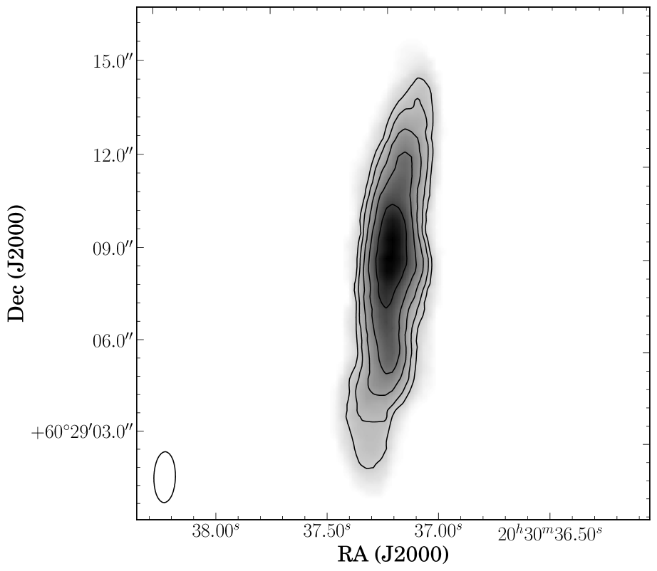
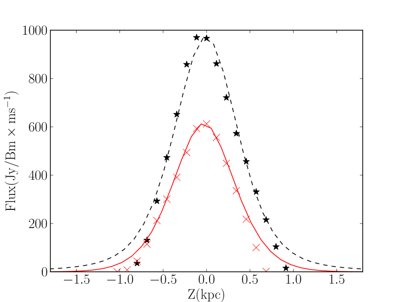
Figure 1: Left Panel GMRT Hi 21 cm radio synthesis image of the dwarf irregular galaxy KK250. The image has been made using an elliptical beam with FWHM $32^{\prime\prime}\times 13^{\prime\prime}$. The contour levels are $(1,1.4,2,2.8,...)~{}5\times 10^{20}$ $\rm atoms~{}cm^{-2}$. See the text for more details. Right Panel This shows the intensity profiles along two vertical cuts through the disc of KK250. The stars are at a galacto-centric distance of 0.1 kpc, while the crosses are at a galacto-centric distance of -1.9 kpc. The dashed and solid lines are the corresponding model profiles at these two locations.

3 Modeling the galactic disc

3.1 Formulation of the Equations

Our model for the galaxy is based on similar modeling of edge-on galaxies done earlier by (Narayan & Jog, 2002; Banerjee & Jog, 2011). Details of the model can be found in those papers, and is also briefly summarized below. The discs of the galaxy are modeled as a 2-component system of gravitationally-coupled stars and gas in the force field of a fixed dark matter halo. We assume that each of the two components is present in a form of a disc, the discs being concentric, and coplanar. We further assume the discs to be axi-symmetric and the halo to be spherically symmetric. The joint Poisson’s equation for the disc plus dark matter halo in cylindrical polar coordinates ($R$, $\phi$, $z$) therefore reduces to

$$\frac{1}{R}\frac{\partial}{\partial R}\left(R\frac{\partial\Phi_{total}}{\partial R}\right)+\frac{\partial^{2}\Phi_{total}}{\partial z^{2}}=4\pi G\left(\sum_{i=1}^{2}\rho_{i}+\rho_{h}\right)$$ (1)

where $\Phi_{total}$ is the total potential due to all the components and dark matter halo. $\rho_{i}$ with $i=s,g$ denotes the mass density of stars and gas respectively. (Following Begum & Chengalur (2004) we correct the observed Hi gas density by a factor of 1.4 to account for the presense of Helium.) $\rho_{h}$ denotes the mass density of the dark matter halo. In their modeling of the rotation curve of this galaxy, Begum & Chengalur (2004) found that the dark matter halo is well fit by a pseudo-isothermal halo, and not well fit by an NFW (Navarro, Frenk, & White, 1996) type halo. We hence take the density distribution in the dark matter halo to be pseudo-isothermal, i.e. with a density profile given by

$$\rho_{h}(R,z)=\frac{\rho_{0}}{1+\frac{R^{2}+z^{2}}{R_{c}^{2}}}$$ (2)

where $\rho_{0}$ and $R_{c}$ are the central core density and core radius respectively (Binney & Tremaine, 1987).

The equation of hydrostatic equilibrium in the $z$ direction for each of the two disc components, is given by

$$\frac{\partial}{\partial z}\left(\rho_{i}{\langle{\sigma}_{z}^{2}\rangle}_{i}\right)+\rho_{i}\frac{\partial\Phi_{total}}{\partial z}=0$$ (3)

where ${\langle{\sigma}_{z}\rangle}_{i}$ is the vertical velocity dispersion of the $i^{th}$ component ($i=s,g$), again an input parameter .

Eliminating ${\Phi}_{total}$ between Equation (1) and (3) we get

$$\begin{split}{\langle{\sigma}_{z}^{2}\rangle}_{i}\frac{\partial}{\partial z}\left(\frac{1}{\rho_{i}}\frac{\partial\rho_{i}}{\partial z}\right)&=-4\pi G\left(\rho_{s}+\rho_{g}+\rho_{h}\right)\\ &+\frac{1}{R}\frac{\partial}{\partial R}\left(R\frac{\partial\phi_{total}}{\partial R}\right)\end{split}$$ (4)

Equation (4) can be further simplified using the fact

$${\left(R\frac{\partial\phi_{total}}{\partial R}\right)}_{R,z}={(v_{rot}^{2})}_{R,z}$$ (5)

Assuming that the vertical gradient in ${(v_{rot})}_{R,z}$ is small, we approximate ${(v_{rot})}_{R,z}$ by the observed rotation curve $v_{rot}$, which is a function of $R$ alone. Thus Equation (4) reduces to

$$\begin{split}{\langle{\sigma}_{z}^{2}\rangle}_{i}\frac{\partial}{\partial z}\left(\frac{1}{\rho_{i}}\frac{\partial\rho_{i}}{\partial z}\right)&=-4\pi G\left(\rho_{s}+\rho_{g}+\rho_{h}\right)\\ &+\frac{1}{R}\frac{\partial}{\partial R}\left(v_{rot}^{2}\right)\end{split}$$ (6)

Therefore Equation (6) now represents two coupled, second-order ordinary differential equations in the variables ${\rho}_{s}$ and ${\rho}_{g}$. The solution of Equation (6) at a given $R$ gives ${\rho}_{s}$ and ${\rho}_{g}$ as a function of $z$ at that $R$. Thus solving Equation (6) at all $R$ gives the model three dimensional density distribution of the stars and gas in the galaxy.

3.2 Input Parameters

As mentioned above, Begum & Chengalur (2004) present mass models for this galaxy, based on the Hi rotation curve. We take the parameters from the mass model of Begum & Chengalur (2004) as inputs to the current model. Specifically, the stellar surface density $\sum_{*}(R)$ is taken to be an exponential with a scale-length $R_{D}$ $\sim\ 1.1$ kpc with the total stellar mass $3.4\times 10^{7}M_{\odot}$. The Hi surface density $\sum_{HI}$ is modeled as a double Gaussian and given by

$${\Sigma}_{HI}={\Sigma}_{01}e^{-r^{2}/2r_{01}^{2}}+{\Sigma}_{02}e^{-r^{2}/2r_{02}^{2}}$$ (7)

with $r_{01}=2.11\pm 0.05$ kpc, $r_{02}=0.41\pm 0.02$ kpc, ${\Sigma}_{01}=5.0\pm 0.1\ M_{\odot}$pc^-2 and ${\Sigma}_{02}=4.2\pm 0.2\ M_{\odot}$pc^-2. As mentioned above, the Hi surface density is scaled to account for the presense of helium to get the total gas density. The dark matter halo is modelled as a pseudo-isothermal halo (Eqn. 2) with $\rho_{0}=37.6\times 10^{-3}\ M_{\odot}$pc^-3 and $R_{c}=1.5$ kpc.

The remaining parameters that need to be specified are the vertical velocity dispersions in the stellar and gaseous discs. These cannot be directly measured from the data for edge-on galaxies. Banerjee & Jog (2011) show that while modelling the structure of the gaseous disc, the accuracy of the assumed value of stellar velocity dispersion ${\sigma}_{z,s}$ has a marginal effect on the calculated Hi scale-height. We hence assume the stellar dispersion ($\sigma_{z,s}$) to be the same as obtained analytically for that of an isothermal stellar disc in vertical hydrostatic equilibrium in the net potential of the stars and the dark matter halo (Leroy et al., 2008). The assumed value of Hi velocity dispersion, ${\sigma}_{g}$ however strongly regulates the calculated Hi scale-height (Banerjee & Jog, 2011). Therefore using an accurate value of ${\sigma}_{g}$ is fundamental to obtaining the correct value of the Hi scale-height. Unlike earlier studies, we have not assumed an ad-hoc value for ${\sigma}_{g}$ for our calculations. Instead, as described below, we have treated ${\sigma}_{g}$ as a free parameter and constrained it using the observed data.

3.3 Solution of the Equations

We solve the two coupled, second-order ordinary differential equations given by Equation (6) in an iterative manner using a Eighth-Order Runge Kutta method as implemented in the scipy package.

$$\left(\rho_{i}\right)_{z=0}=\rho_{i,0}\ \ \ \ {\rm and}\ \ \ \frac{d\rho_{i}}{dz}=0$$ (8)

The observations constrain the observed surface density ${\Sigma}_{i}$ and not the midplane density $\rho_{i,0}$. We hence take a trial value of $\rho_{i,0}$, and iterate until the model matches the observed $\Sigma_{i}$. We are able to measure the Hi vertical distribution only within a projected galacto-centric radius of 3 kpc, beyond that the signal to noise ratio is too poor to allow a realiable estimate to be made. Accordingly we solve Equation (6) for 0 $<$ $R$ $<$ 3 kpc at steps of 100 pc in the radial direction, and an adaptive (scale-height sensitive) resolution along the vertical axis. The resolution along the vertical direction was always better than 10 pc. The solution at the intermediate radii is estimated by interpolation. Since $v_{rot}$ is fixed, Equation(6) can be solved independently for each value of the radius $R$. Instead of assuming a fixed value of $\sigma_{g}$ at each $R$, we treat it as a free parameter satisfying the following two constraints: (i) 1 $<$ ${\sigma}_{g}$ $<$ 24 kms^-1(ii) ${\sigma}_{g}$ does not increase with $R$. The upper limit of $\sim 24$ kms^-1was set by increasing the upper limit to the range of $\sigma_{g}$ being searched until we found a value that bracketed the best fit $\sigma_{g}$. We then explored the entire available parameter space in velocity dispersion using a grid with cell size in velocity of 2 kms^-1and radial cell size of 500 pc. In practice we generated a set of solutions for $\rho_{i}(R,z)$; each solution was for a fixed value of $\sigma_{g}$, with the $\sigma_{g}$ being varied in steps of 2 kms^-1between the different solutions. Combinations of these solutions were then made for all possible $\sigma_{g}$ profiles that satisfy the constraints listed above. Since, as noted earlier, Eqn(6) needs to be solved only as a function of $z$, combining the solutions is equivalent to solving the equation for each possible $\sigma_{g}$ profile. From the $\rho_{g}(R,z)$ and the rotation curve we constructed a 3D model of the galaxy. This was then projected to the adopted morphological inclination ($i$ = $85^{o}$, see the discussion below), and convolved with the telescope beam to produce a model data cube.

Begum & Chengalur (2004) estimated the morphological inclination to be $i$ = $80^{o}\pm 4^{o}$. A value of $80^{o}$ for the inclination requires an extremely large velocity dispersion ($\sigma_{g}\sim 40$ kms^-1) at the centre to reproduce the observed morphology. In deriving the inclination, Begum & Chengalur (2004) assumed the intrinsic axial ratio to be $q_{0}$ = 0.2, however Roychowdhury et al. (2013) show that dwarf galaxies tend to have somewhat larger intrinsic axial ratios. For galaxies with luminosity M_B between $-12.6$ and $-14.8$ the mean axial ratio is $0.36$ with a scatter of $\sim 0.15$. A larger intrinsic axial ratio would lead to a higher value of the inclination. The inclination adopted here ($i=85^{o}$) is consistent with this expectation. We note however that there is some uncertainty in deriving inclinations of dwarf galaxies, and our adopted value is in some sense a best guess.

Since the Hi emission is optically thin, the integrated Hi flux image has folded into it the distribution of all of the gas along the given line of sight. This means that for an edge on galaxy there is no one to one mapping between the observed thickness of the Hi distribution at a given projected galacto-centric radius and the intrinsic Hi scale-height. In order to compare the model distribution with the observations, we hence generate a model integrated flux image from the model data cube and measure the FWHM of the Hi vertical distribution computed in exactly the same way as was done with the observed “moment 0” image. The $\sigma$ profile that produced the best fit (smallest $\chi^{2}$) fit to the observed data was picked as the best fit model. This is the most compute intesive step of the model fitting, and it was implemented using MPI based code and run on a 32 node IBM sandybridge cluster. A run using 400 processors takes about 8 hours. The best fit model had $\sigma_{g}$ tending to a constant value of $8$ kms^-1outside of $R\geq 1.5$ kpc, and rises steeply inside this. To resolve this better, a second set of models were produced, with $\sigma_{g}$ set to $8$ kms^-1outside $R=1.5$ kpc, and with $\sigma$ varying from $7-24$ km/s inside. The cells of fixed $\sigma_{g}$ were reduced to 300 pc instead of the earlier value of 500 pc. The best fit of these models is then picked as our final model.

4 Results and Discussion

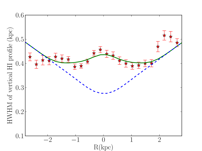
Figure 2: Plot of the obseved (points with error bars) half-width-at-half-maxima (HWHM) of the Hi vertical intensity profile of the edge-on dwarf irregular galaxy KK250 as a function of galactocentric radius $R$ overlaid with the best fit model (solid line), as well as a model in which the gas velocity dispersoion, $\sigma_{g}$ is fixed at 8 kms^-1(blue dashed line).

In Fig. 2, we compare the half-width-at-half-maximum (HWHM) of the observed vertical Hi intensity distribution (points with error bars) with that from the best fit model (solid line). For comparison we also plot the HWHM profile for the constant $\sigma_{g}=8$ kms^-1model (blue dashed line). As can be seen, the match between our model and the data is excellent inside a galacto-centric radius of 2 kpc. Between 2 kpc and 3 kpc the observed disc is slightly asymmetric. In this region one can see that the model represents some kind of average of the two halves. The model with constant $\sigma_{g}=8$ kms^-1fails to produce the observed HWHM profile at the central region of the galaxy, though it merges with our model at $\sim R>2$ kpc.

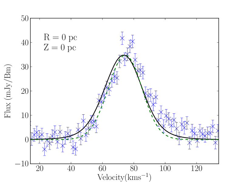
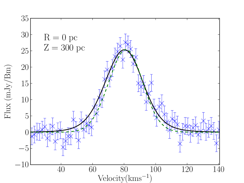
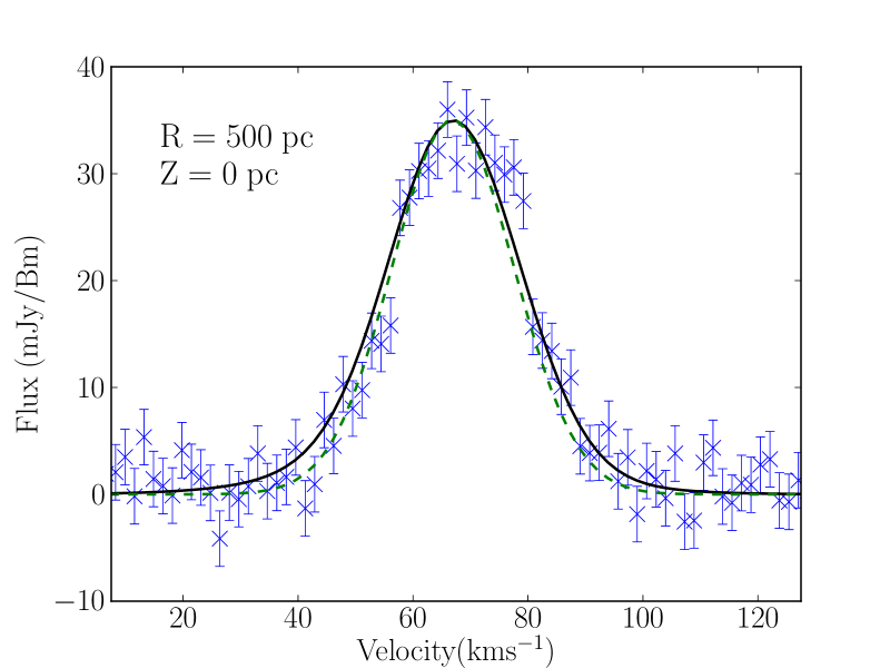
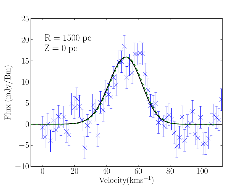
Figure 3: Observed versus model Hi spectra at different locations in the galaxy. The solid and dotted lines show the best fit model and a model with a constant velocity dispersion of 8 kms^-1respectively. The model was fit only using the morphological data and not the kinematical data. Comparison of the model and observed spectra is hence an independent cross check of the model.

In Fig. 3 we compare the observed velocity profiles with the model profiles. Since the aim of this exercise is to see if the data provides some independent support for the existence of high velocity dispersion gas in the central regions of the galaxy, we have slightly shifted and scaled the model spectra so that they align exactly with the observed spectra. Recall that our model fitting used only the morphological data, this comparison provides an independent check. As can be seen from the figure, the velocity profiles in the central regions of the galaxy show an excess flux at $v\sim 100$ kms^-1as compared to the best fit model spectrum. This could perhaps be due to some low level non-circular motions which are not captured in our model. Several mechanism like feedback from star-formation, inflow or outflow of gas from the central region etc. could lead to this kind of non-circular motion. We also note in passing that the total amount of gas with high velocity dispersion is relatively small, and the existence of this gas is difficult to determine from the moment 2 maps that are often used as a measure of the velocity dispersion.

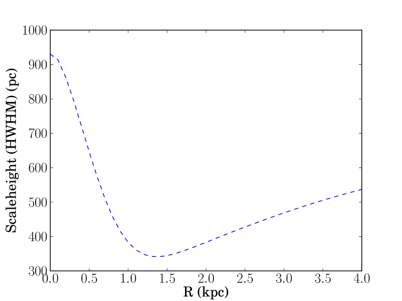
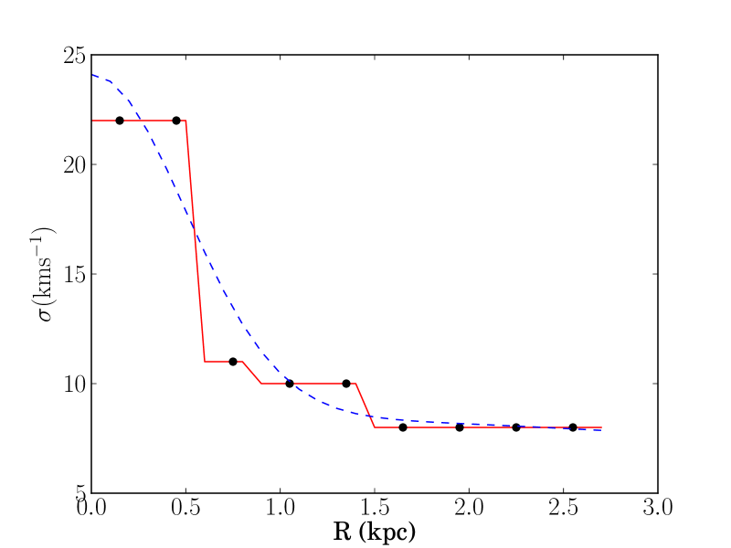
Figure 4: Left Panel: Plot of the calculated intrinsic scale-height (half-width-at-half-maxima) versus $R$ corresponding to the Gaussian fits to the best-fit $\sigma_{g}$ profile. Right Panel: Best-fit intrinsic Hi velocity dispersion ${\sigma}_{g}$ versus $R$ overlaid with a double gaussian fit to the same. The velocity dispersion ${\sigma}_{g}$ takes a value of $\sim$ 22 kms^-1at the galaxy centre and falls steeply with increasing galacto-centric radius $R$ reaching to $\sim 8$ kms^-1beyond $R$ $\sim$ 1 kpc.

As discussed above, since the Hi is optically thin, the observed vertical distribution of the Hi reflects the scale-height distribution of all of the gas along the line of sight. If the scale-height does not vary with radius then the observed vertical distribution can be used to determine the intrinsic scale-height of the gas. If the scale-height varies with radius then determination of the true scale-height from the observed vertical distribution is not so straight forward. In the current case, since we have modelled the galaxy, we can use the model to determine how the scale-height varies with radius. In Fig. 4 (Left Panel), we plot the calculated model scale-height (defined as the HWHM of the model Hi vertical density profile) versus $R$ for the best-fit ${\sigma}_{g}$ profile. As can be seen the HWHM varies significantly with galacto-centric radius. At $R$ $\sim$ 0, the HWHM is $\sim$ 700 pc, it drops to a minimum value of $\sim$ 350 pc at $R$ = 1 kpc. This is similar to both the scale-length of the stellar disc, as well as the spatial resolution of the data along the galaxy major axis. Beyond 1 kpc the gas disc flares by almost a factor of 2 by $R$ = 4 kpc. Hi flaring in the outer parts of galaxies is a common phenomenon and can be attributed to the decreasing importance of the self gravity of the disc components (see for example the study by Banerjee & Jog, 2011). However the large HWHM seen in the central regions of the galaxy is unusual. To understand this better, it is useful to look at the radial variation of the velocity dispersion in our best fit model. In Fig. 4 (Right Panel), we plot our best-fit ${\sigma}_{g}$ versus $R$ along with a double-gaussian fit to the same. The velocity dispersion at the center of the galaxy is $\sim 22$ kms^-1and it falls steeply to a value of 8 kms^-1by $R$ $\sim$ 1 kpc, which is equal to one exponential stellar disc scale-length $R_{D}$ . The earlier studies (Banerjee & Jog, 2011) of the scale-height in dwarf galaxies assumed a constant velocity dispersion of $\sigma_{g}=8$ kms^-1. In Figure 2 we show the HWHM derived from a model in which we have assumed $\sigma_{g}=8$ kms^-1. As can be seen, this provides a poor fit to the data in the central regions of the galaxy. Clearly the high velocity dispersion in the best fit model is driven by the fact that the observed HWHM is roughly constant towards the center of the galaxy, while the vertical gravitational force gets larger as one approaches the galaxy center. The decrease in velocity dispersion as one goes from the center to the edge of the disc in KK250 is also consistent with earlier results that in most galaxies the velocity dispersion either remains constant or decreases with radius (Tamburro et al., 2009). Our inferred value of ${\sigma}_{g}$ of 22 kms^-1at the centre of galaxy is however somewhat high compared to the typical values obtained from other studies of dwarf galaxies. For e.g. Johnson et al. (2012) find ${\sigma}_{g}$ $\sim$ 10 kms^-1for galaxies in the LITTLE THINGS survey and Stilp et al. (2013) obtain values $\sim$ 6 - 12 kms^-1for the dwarf irregulars in the Local Group. We note however that apart from the center most region, the velocity dispersion in KK250 is similar to the values reported in these other works.

One of the input parameters to our model was the mass distribution as derived from the rotation curve by Begum & Chengalur (2004). In that paper the asymmetric drift correction (viz. the correction for the support against collapse provided by the pressure gradient in the gas) was derived by assuming the velocity dispersion to have a constant value of 8 kms^-1. Since the value we get near the centre of the galaxy is somewhat higher, we recalculated the asymmetric drift-corrected rotation curve using the velocity dispersion as estimated here. The corrected curve lies within the error bars of the original rotation curve of Begum & Chengalur (2004), which justifies the use of the mass decomposition derived in that paper.

What is the origin of the velocity dispersion that we observe? The one dimension thermal velocity dispersion associated with 8000 K gas (i.e. a reasonable upper limit to the kinetic temperature of the Warm Neutral Medium) is $\sim 8$ kms^-1. So while it is possible that the velocity dispersion that we see in the outer parts of the galaxy are entirely due to thermal motions of the particles, in central regions there must be an extra contribution due to small scale bulk motions of the gas. Velocity spreads in excess of thermal in the neutral ISM are often attributed to turbulence. In the case of dwarf galaxies, further evindence for the exisitence of turbulence in the atomic ISM comes from studies of the power spectrum of the Hi intensity fluctuations (Begum, Chengalur, & Bhardwaj, 2006; Dutta et al., 2009; Block et al., 2010; Dutta et al., 2013). Turbulence in the atomic gas in galaxies can arise from energy input from star formation and supernovae explosions (Mac Low & Klessen, 2004), magneto-rotational instabilities (MRI) in differentially rotating discs, (Sellwood & Balbus, 1999), gravitational instabilities (Wada, Meurer, & Norman, 2002) and mass accretion Klessen & Hennebelle (2010). KK250 has a linearly rising rotation curve, and hence the magneto-rotational instability does not appear to be relevant here. KK250 has a nearby companion dwarf galaxy, KK251, and tidal interaction could be a possible reason for the increased velocity dispersion. However, the Hi distributions of KK250 and KK251 show no obvious sign of interaction or disturbance, and the rotation curves of the galaxies also appear fairly regular (Begum & Chengalur, 2004). It is hence appears that tidal interactions may not be playing an important role in this system. Which, if any, of the remaining mechanisms are responsible for driving turbulence in dwarf irregulars is currently unclear (see for e.g. Stilp et al., 2013).

Regardless of the origin of the velocity dispersion, the fact that the estimated velocity dispersion in dwarfs is comparable to that in much larger spiral galaxies will have consequences for the structures of the gaseous discs in dwarfs. The larger ratio of ${\sigma}_{g}/v_{\rm rot}$ in dwarfs will lead to their gas discs being thicker that those of spiral galaxies. Indeed, the typical HWHM for the Hi that we determine for KK250 is significantly larger than the value of $\sim 70-140$pc determined for the inner disc of the Milky way (Malhotra, 1995). Similarly large scale-heights for dwarf galaxies have also been indicated by studies of the power spectrum of the Hi intensity fluctuations (Dutta et al., 2009). These results are based on the expectation that the slope of the power spectrum will change on scales comparable to the scale-height of the galaxy (Elmegreen, Kim, & Staveley-Smith, 2001). Finally, studies of the axial ratio distribution of the gas and stellar discs of dwarf galaxies (Roychowdhury et al., 2010, 2013) do indeed show that their stellar and gaseous discs are significantly thicker than those of spirals. The more diffuse gas distribution has several implications for galaxy evolution, including being likely to be one of the causes for the observed low efficiency of conversion of stars to gas in dwarf galaxies (Roychowdhury et al., 2009, 2011).

5 Conclusion

We use GMRT Hi 21cm observations of the dwarf irregular galaxy KK250 to model the vertical distribution of the atomic gas. Our model consists of a 2-component galactic disc model of gravitationally-coupled stars and gas in the force field of a dark matter halo. The dark matter halo parameters are derived from fitting to the observed rotation curve. We allow the velocity dispersion of the gas to be a free parameter in the model, and constrain it using the observed half width half maximum of the vertical distribution of the Hi. For the best fit model we also compare the observed line of sight velocity widths with the model ones, and find the two to be in good agreement. This provides a further consistency check to the derived velocity dispersion. From our best fit model, we find that the velocity dispersion is maximum at the center, but rapidly falls to a value of $\sim 8$ kms^-1at $R\sim 1$ kpc. This is similar to both the scale-length of the stellar disc, as well as the spatial resolution along the radial direction. The intrinsic Hi scale-height also reaches its minimum value at $R\sim 1$ kpc. The scale-height that we measure for KK250 is significantly larger than the scale-height of the Hi in the central regions of the Milk way, consistent with earlier observations that dwarf galaxies have significantly thicker gas discs than typical spiral galaxies.

References

- Banerjee & Jog (2011) Banerjee A., Jog C. J., 2011, ApJ, 732, L8
- Banerjee, Matthews, & Jog (10) Banerjee A., Matthews L. D., Jog C. J., 2010, NewA, 15, 89
- Banerjee & Jog (2008) Banerjee A., Jog C. J., 2008, ApJ, 685, 254
- Becquaert & Combes (1997) Becquaert J.-F., Combes F., 1997, A&A, 325, 41
- Begum et al. (2008) Begum A., Chengalur J. N., Karachentsev I. D., Sharina M. E., Kaisin S. S., 2008, MNRAS, 386, 1667
- Begum, Chengalur, & Bhardwaj (2006) Begum A., Chengalur J. N., Bhardwaj S., 2006, MNRAS, 372, L33
- Begum & Chengalur (2004) Begum A., Chengalur J. N., 2004, A&A, 424, 509
- Binney & Tremaine (1987) Binney, J., Tremaine, S. 1987, Galactic Dynamics, Princeton Univ. Press, Princeton, NJ
- Block et al. (2010) Block D. L., Puerari I., Elmegreen B. G., Bournaud F., 2010, ApJ, 718, L1
- Dutta et al. (2013) Dutta P., Begum A., Bharadwaj S., Chengalur J. N., 2013, NewA, 19, 89
- Dutta et al. (2009) Dutta P., Begum A., Bharadwaj S., Chengalur J. N., 2009, MNRAS, 398, 887
- Elmegreen, Kim, & Staveley-Smith (2001) Elmegreen B. G., Kim S., Staveley-Smith L., 2001, ApJ, 548, 749
- Johnson et al. (2012) Johnson M., Hunter D. A., Oh S.-H., Zhang H.-X., Elmegreen B., Brinks E., Tollerud E., Herrmann K., 2012, AJ, 144, 152
- Karachentsev, Makarov, & Kaisina (2013) Karachentsev I. D., Makarov D. I., Kaisina E. I., 2013, AJ, 145, 101
- Klessen & Hennebelle (2010) Klessen R. S., Hennebelle P., 2010, A&A, 520, A17
- Leroy et al. (2008) Leroy A. K., Walter F., Brinks E., Bigiel F., de Blok W. J. G., Madore B., Thornley M. D., 2008, AJ, 136, 2782
- Mac Low & Klessen (2004) Mac Low M.-M., Klessen R. S., 2004, RvMP, 76, 125
- Malhotra (1995) Malhotra S., 1995, ApJ, 448, 138
- Narayan, Saha, & Jog (2005) Narayan C. A., Saha K., Jog C. J., 2005, A&A, 440, 523
- Narayan & Jog (2002) Narayan C. A., Jog C. J., 2002, A&A, 394, 89
- Navarro, Frenk, & White (1996) Navarro J. F., Frenk C. S., White S. D. M., 1996, ApJ, 462, 563
- Olling (1995) Olling R. P., 1995, AJ, 110, 591
- Roychowdhury et al. (2013) Roychowdhury S., Chengalur J. N., Karachentsev I. D., Kaisina E. I., 2013, MNRAS, 436, L104
- Roychowdhury et al. (2011) Roychowdhury S., Chengalur J. N., Kaisin S. S., Begum A., Karachentsev I. D., 2011, MNRAS, 414, L55
- Roychowdhury et al. (2010) Roychowdhury S., Chengalur J. N., Begum A., Karachentsev I. D., 2010, MNRAS, 404, L60
- Roychowdhury et al. (2009) Roychowdhury S., Chengalur J. N., Begum A., Karachentsev I. D., 2009, MNRAS, 397, 1435
- Stilp et al. (2013) Stilp A. M., Dalcanton J. J., Skillman E., Warren S. R., Ott J., Koribalski B., 2013, ApJ, 773, 88
- Sellwood & Balbus (1999) Sellwood J. A., Balbus S. A., 1999, ApJ, 511, 660
- Swarup et al. (1991) Swarup G., Ananthakrishnan S., Kapahi V. K., Rao A. P., Subrahmanya C. R., Kulkarni V. K., 1991, CuSc, 60, 95
- Tamburro et al. (2009) Tamburro D., Rix H.-W., Leroy A. K., Mac Low M.-M., Walter F., Kennicutt R. C., Brinks E., de Blok W. J. G., 2009, AJ, 137, 4424
- Wada, Meurer, & Norman (2002) Wada K., Meurer G., Norman C. A., 2002, ApJ, 577, 197