Exact results for models of multichannel quantum nonadiabatic transitions

Abstract

We consider nonadiabatic transitions in explicitly time-dependent systems with Hamiltonians of the form $\hat{H}(t)=\hat{A}+\hat{B}t+\hat{C}/t$, where $t$ is time and $\hat{A}$, $\hat{B}$, $\hat{C}$ are Hermitian $N\times N$ matrices. We show that in any model of this type, scattering matrix elements satisfy nontrivial exact constraints that follow from the absence of the Stokes phenomenon for solutions with specific conditions at $t\rightarrow-\infty$. This allows one to continue such solutions analytically to $t\rightarrow+\infty$, and connect their asymptotic behavior at $t\rightarrow-\infty$ and $t\rightarrow+\infty$. This property becomes particularly useful when a model shows additional discrete symmetries. In particular, we derive a number of simple exact constraints and explicit expressions for scattering probabilities in such systems.

I Introduction

Quantum nonadiabatic transitions have been studied for a long time with numerous applications in physics of atomic and molecular collisions book . This field of research has strongly benefited from the discovery of exact formulas that describe dynamics of two-state systems in specific but frequently encountered situations. The most famous such a theoretical result is the Stueckelberg-Majorana-Landau-Zener (LZ) formula maj ; landau ; LZ . However, many other exact results, such as the solution of the Rosen-Zener model and its generalizations rozen ; nikitin ; osherov , have also been very influential and frequently used.

More recently, the interest in quantum nonadiabatic transitions has been revived due to the new applications in ultra-cold atomic systems app-bose ; chain1 , quantum coherence coher , Landau-Zener interferometry LZ-interferometry , and quantum control of mesoscopic systems qcontrol , which typically deal with quantum systems of mesoscopic size and a large phase space.

The multistate version of the LZ model is one of the most frequently emerging problems in these studies book . It considers interactions among $N$ states during the time evolution described by the Schödinger equation with time-dependent parameters that change according to simple power laws. Specifically, here we will discuss the evolution equations of the form:

$$i\frac{d\psi}{dt}=\left(\hat{A}+\hat{B}t+\frac{\hat{C}}{t}\right)\psi,$$ (1)

where $\psi$ is the state vector in a space of $N$ states; $\hat{A}$, $\hat{B}$ and $\hat{C}$ are constant Hermitian $N\times N$ matrices.

In this article, we will assume that matrices are written in the, so-called, diabatic basis, in which the matrix $\hat{B}$ is diagonal and if some of its diagonal elements $\beta_{i}$, $i=1,\ldots,N$, are degenerate then diabatic basis states are chosen to make constant couplings among such states equal to zero, i.e. in the diabatic basis we have:

$$\hat{B}={\rm diag}\{\beta_{1},\ldots\beta_{N}\},\quad A_{nm}=0\,\,\,{\rm if}\,\,\,\beta_{n}=\beta_{m}.$$ (2)

Diagonal elements of the Hamiltonian

$$\hat{H}(t)=\hat{A}+\hat{B}t+\hat{C}/t$$ (3)

can be generally written in the diabatic basis as

$$\varepsilon_{i}^{d}=\beta_{i}t+\epsilon_{i}+k_{i}/t,\quad i=1,\ldots N,$$ (4)

where $k_{i}$ are diagonal elements of $\hat{C}$ and $\epsilon_{i}$ are diagonal elements of $\hat{A}$. Off-diagonal elements of $\hat{A}$ and $\hat{C}$ in the diabatic basis are called the coupling constants.

The goal of the theory is to find the scattering $N\times N$ matrix $\hat{S}$, whose element $S_{nn^{\prime}}$ is the amplitude of the diabatic state $n$ at $t\rightarrow+\infty$, given that at $t\rightarrow 0_{+}$ the system was in the $n^{\prime}$-th eigenstate of the Hamiltonian. In most cases, only the related matrix $\hat{P}$, $P_{n^{\prime}\rightarrow n}=|S_{nn^{\prime}}|^{2}$, called the matrix of transition probabilities, is of interest.

Even the case of Eq. (1) for only two states ($N=2$) generally does not reduce to the hypergeometric equation, and its analytical solution, e.g. in the form of a contour integral of a simple function, is unknown. Situation may look even less promising at larger $N$ because Eq. (1) is then equivalent to an $N$-th order differential equation with polynomial time-dependent coefficients that quickly grow in complexity.

Although the general solution of the model (1) has not been found, a number of exactly solvable cases with specific forms of matrices $\hat{A}$, $\hat{B}$ and $\hat{C}$ have been derived. Exact results provided useful intuition about the behavior of strongly driven quantum systems. The models of type (1) with $\hat{C}=0$ have been discussed rather extensively in the past be ; shytov ; no-go ; mlz-1 ; do ; reducible ; bow-tie ; chain . In contrast, the addition of the last term in (1), with $\hat{C}\neq 0$, has been introduced relatively recently in physics literature coulomb1 , and it will be the main focus of the present work.

We will refer to an arbitrary model of the type (1) with a nonempty matrix $\hat{C}$ as an LZC-model, named after Landau, Zener and Coulomb. Exactly solvable LZC models have been shown to capture very complex patterns of behavior, including counterintuitive transitions and wild oscillations of transition probabilities as functions of parameters sinitsyn-13prl ; sinitsyn-13jpa ; sinitsyn-14jpa . Physically, they show a lot of common features with nonadiabatic transitions in Rydberg atoms stark and molecular collision models singular .

The goal of this article is to explore an unusual phenomenon that appears to be common for all models of the type (1). We will demonstrate that no matter how big is the complexity of such a model, there are always nontrivial but simple exact constraints on its scattering matrix elements in addition to the trivial constraints that follow from the unitarity and elementary discrete symmetries. We will provide tests of such constraints by numerical simulations and comparisons with available exact results, and demonstrate how they can be used to derive new relations between transition probabilities in specific systems.

The structure of our article is as follows. In section 2, we will explore the Stokes phenomenon in systems of the type (1) and derive the exact constraints for the scattering matrix for such systems. In section 3, we explore the case $N=2$ in more detail and demonstrate how constraints on the scattering matrix can lead to constraints on transition probabilities in elementary LZC-type models. Section 4 describes specific examples with $N>2$ for which simple constraints on transition probabilities can be derived. We summarize our results in the conclusion section 5, in which we also discuss possible directions for the future research. Appendix A connects our results with previous studies of the special case of $\hat{C}=0$ in (1). Appendix B presents the derivation of exact transition probabilities in a specific model with arbitrary $N$ that we use to check the validity of some of our results in the main text.

II Asymptotic behavior of extremal amplitudes in LZC models

Our treatment of the general case of the LZC model will closely follow the proof of the Brundobler-Elser formula and derivation of the no-go theorem in no-go . The major difference from that work is that now we include a nonzero value of the matrix $\hat{C}$ into account. Let us define the extremal amplitude as the amplitude of the diabatic state that has the highest or the lowest slope at $t\rightarrow\pm\infty$ i.e. that has the largest or the lowest eigenvalue of the matrix $\hat{B}$.

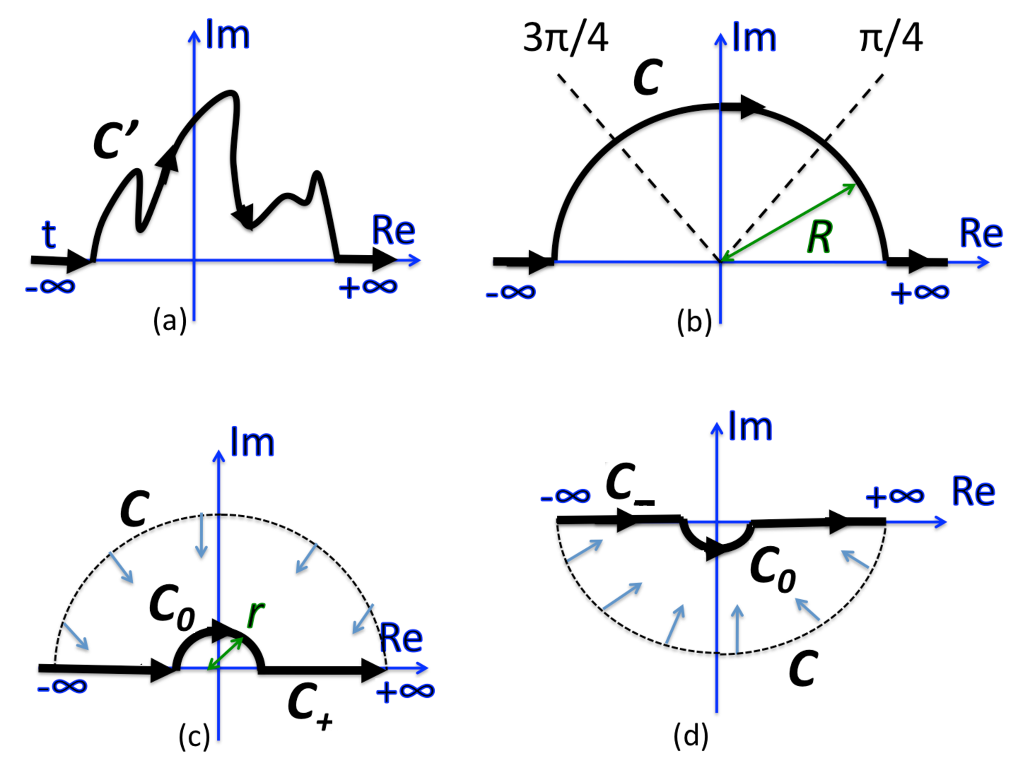
Figure 1: Contours of complex time for evolution with Eq. (1) connecting real points at $t\rightarrow\pm\infty$. (a) Arbitrary contour ${\bm{C}^{\prime}}$ laying in the upper half plane can be deformed without encountering singularities into the contour ${\bm{C}}$ shown in (b) that has the shape of a semicircle with radius $R$. This contour crosses two rays, $t=Re^{i\phi}$, at $\phi=3\pi/4$ and $\phi=\pi/4$. Along those rays, the highest slope amplitude has the highest rate of, respectively, decay and growth with increasing $R$. (c) Without changing asymptotic values of the solution at real $t\rightarrow\pm\infty$, the contour ${\bm{C}}$ can be deformed to the contour that is placed almost everywhere on the real time axis, except an infinitely small semicircle that avoids the singularity of the Hamiltonian (3) at $t=0$. (d) Applying the same arguments to the extremal amplitude with the lowest slope of diabatic energy, we arrive at a contour ${\bm{C}}$ at the lower complex half-plane that can be deformed to a contour along the real axis except an infinitely small semicircle around $t=0$ in the lower half-plane.

We can now prove the following rule:

II.1 Connection formula

Without loss of generality, let $1$ be the index of the extremal slope with $\beta_{1}=\max(\beta_{1}\ldots\beta_{N})$ and let ${\bm{C}^{\prime}}$ be an arbitrary contour that connects asymptotic values $t\rightarrow\pm\infty$ on the real axis but otherwise it makes arbitrary continuous path in the upper half of the complex plain avoiding the singular point of the Hamiltonian at $t=0$, as shown in Fig. 1(a). Suppose also that at real $t\rightarrow-\infty$ the asymptotic values of the amplitudes of diabatic states are given by

$$|\psi_{1}^{-\infty}(t)|=1,\quad|\psi_{i}^{-\infty}(t)|=0,\quad i\neq 1.$$ (5)

We are going to show now that the value of the extremal amplitude at real $t\rightarrow+\infty$ is given by

$$\psi_{1}^{+\infty}(t) = S^{\rm up}_{11}\psi_{1}^{-\infty}(t),$$ (6)

$$S^{\rm up}_{11} = \exp\left(-\pi k_{1}-\pi\sum\limits_{i\,(i\neq 1)}\frac{|A_{1i}|^{2}}{|\beta_{1}-\beta_{i}|}\right),$$ (7)

where parameters are introduced in Eqs. (1)-(4), and index “up” indicates that evolution went along the time contour in the upper half of the complex plane.

Respectively, let $N$ be the index of the extremal slope with $\beta_{N}=\min(\beta_{1}\ldots\beta_{N})$ and ${\bm{C}^{\prime}}$ connects real $t\rightarrow\pm\infty$ in the lower half of the complex plane with initial conditions

$$|\psi_{N}^{-\infty}(t)|=1,\quad|\psi_{i}^{-\infty}(t)|=0,\quad i\neq N,$$ (8)

then

$$\psi_{N}^{+\infty}(t) = S^{\rm dn}_{NN}\psi_{N}^{-\infty}(t),$$ (9)

$$S^{\rm dn}_{NN} = \exp\left(+\pi k_{N}-\pi\sum\limits_{i\,(i\neq N)}\frac{|A_{Ni}|^{2}}{|\beta_{i}-\beta_{N}|}\right),$$ (10)

where the index “dn” indicates that evolution went along the time contour in the lower half of the complex plane.

Proof: Consider nodegerate $\beta_{i}$, $i=1,\ldots N$. We will prove the case of the highest slope first. Since we are interested in the asymptotic magnitude of the amplitudes of states at large time, we do not have to find the evolution matrix for Eq. (1) at arbitrary time point of ${\bm{C}^{\prime}}$. Moreover, since the solution is analytic everywhere except $t=0$, the deformations of the contour that do not change its asymptotic poins at the real axis do not change asymptotics of the solution. Hence, we can analytically extend the evolution (1) to the path ${\bm{C}}$ that always has $|t|\rightarrow\infty$, as shown in Fig. 1(b) i.e.

$${\bm{C}}:t=Re^{i\phi}\quad R\rightarrow\infty,\quad\phi\in[\pi,0],$$ (11)

where $R$ is real and positive.

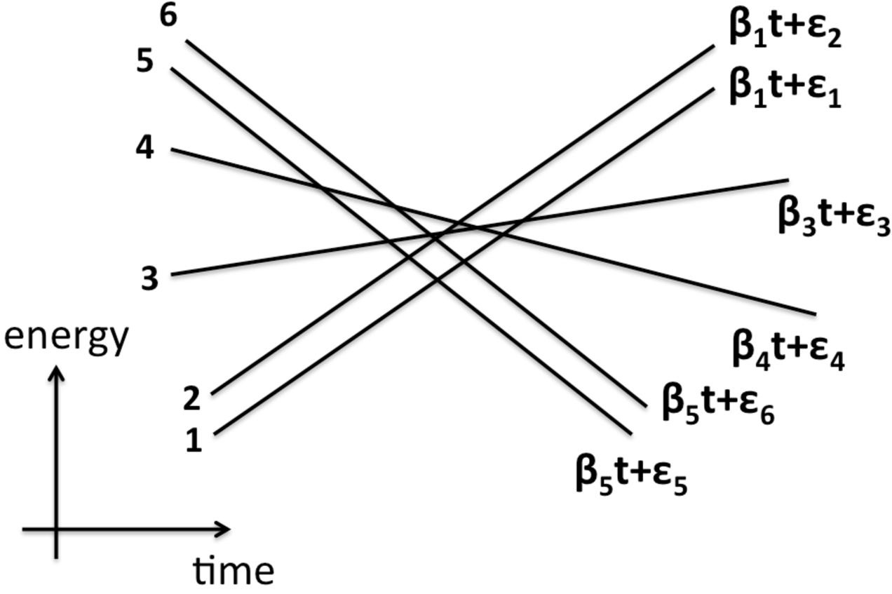
Figure 2: Plot of diagonal elements of the matrix $\hat{B}t+\hat{A}$ in the diabatic basis can be used to identify extremal states and counterintuitive transitions. For the shown system of six states, levels 1 and 2 have the highest slope, levels 5 and 6 have the lowest slope, and transitions from level 6 to level 5 and from level 1 to level 2 are counterintuitive.

Along the contour ${\bm{C}}$, diabatic states coincide with eigenstates of the Hamiltonian. The distances between corresponding instantaneous eigenenergies $E_{i}(t)$ of the Hamiltonian (3) remain always large in this case, namely of the order of $|(\beta_{i}-\beta_{j})t|>>|A_{ij}|,\,|C_{ij}/t|$ for the states $i\neq j$ and hence one can use the adiabatic approximation for the amplitudes $\psi_{i}$ of the diabatic states:

$$\psi_{i}(t)=e^{-i\int_{-\infty}^{t}E_{i}(t)dt}\psi_{i}(-\infty),\quad i=1,\ldots,N.$$ (12)

To the leading orders in $1/R$, the Hamiltonian eigenenergy that corresponds to the amplitude of the highest slope is given by

$$E_{1}=\beta_{1}t+\frac{1}{t}\left(k_{1}+\sum\limits_{j\,(j\neq 1)}\frac{|A_{1j}|^{2}}{|\beta_{1}-\beta_{j}|}\right)+O(1/R^{2}).$$ (13)

Now, as it was done in shytov ; no-go for the case of $\hat{C}=0$, we make the observation that by substituting (13) into (12) and integrating over time along the semi-cycle $t=Re^{i\phi}$, where $\phi\in[\pi,0]$, we obtain (7).

This observation, however, cannot be considered as the proof yet because, generally, the adiabatic approximation (12) may break down for complex values of time, which is the essence of the Stokes phenomenon. The evolution along a complex time path is no longer unitary so that some of the amplitudes can become exponentially large in comparison to $\psi_{k}$. In such a case, approximation (12) cannot be applied because even a weak coupling to states with exponentially large amplitudes cannot be treated perturbatively.

In principle, to justify (12), one can apply arguments akin to Landau’s derivation of the LZ-formula and the treatment of over-barrier transitions landau , as it was suggested in shytov for systems with $\hat{C}=0$. However, such arguments are intrinsically semiclassical and generally predict only the leading exponential factor for a transition amplitude. For example, the semiclassical formula for the over-barrier reflection fails in the limit of a weak barrier, i.e. in the domain of applicability of the Born approximation. In order to make exact statements, one has to explore the Stokes phenomenon in this problem in more detail.

In order to prove that the perturbative expansion (13) can be used in Eq. (12) everywhere along the path ${\bm{C}}$, we should show that the amplitude with energy $E_{1}$ remains either exponentially larger or at least of the same order with other state amplitudes. The latter means here that the ratio of the extremal amplitude to any other one is not suppressed exponentially in the limit $R\rightarrow\infty$.

It is sufficient for this proof to consider only the leading order terms in the exponents

$$\psi_{i}\sim\exp(-i\beta_{i}t^{2}/2),\quad i=1,\ldots,N.$$ (14)

Stokes phenomenon, i.e. sharp changes of the behavior of the values of the amplitudes at $R\rightarrow\infty$, can happen at crossing the Stokes lines, i.e. rays along which some of the amplitudes are growing/decaying with extremal rate. In our case, those lines are the rays $\phi=\pi/4$ and $\phi=3\pi/4$. It is sufficient to prove that the extremal amplitude behaves continuously at crossing those rays.

Consider the ray at $\phi=3\pi/4$ and assume that $\psi_{1}$ is of the same order or exponentially larger than all other state amplitudes at some very large $R$. This is the ray of the slowest growth of the extremal amplitude. Hence, by continuing asymptotics (14) to larger values of $\phi$, the amplitude $\psi_{1}$ is exponentially growing in comparison to all other amplitudes up to $\phi=\pi$. This means that this solution can be normalized to satisfy initial conditions (5) and the extremal amplitude does not become suppressed in comparison to other states in the sector ($\pi,3\pi/4$). Similarly, moving to the right from the ray $\phi=3\pi/4$, we find that up to the ray $\phi=\pi/4$, the amplitude $\psi_{1}$ is exponentially growing in comparison to other amplitudes. Finally, at interval $\phi\in(\pi/4,0)$ other amplitudes start growing but from exponentially suppressed value at $\phi=\pi/4$. Therefore, it is safe to continue the extremal amplitude analytically to the right of this ray and hence to the whole sector up to $\phi=0$. This completes our proof of the absence of the Stokes phenomenon for the extremal amplitude along the contour ${\bm{C}}$ and initial conditions (5). The proof for the level with the lowest slope is analogous but with the contour ${\bm{C}}$ placed in the lower half of the complex plane.

II.2 No-Go Rule for LZC models

Equations (7) and (10) are generalizations of the Brundobler-Elser formula in multi-state Landau-Zener models with linear time dependence of parameters, which we review briefly in Appendix A. Our inclusion of the Coulomb term in (1) changed the result but did not change basic steps discussed in no-go for derivation of the connection formula for the case $\hat{C}=0$. Indeed, at large time values, the Coulomb term introduces only marginally relevant contribution, which produces a geometric-phase-like pre-factor, which does not influence the Stokes phenomenon. This observation can be used to derive another exact constraint. Namely, in no-go , the so-called “No-Go Rule” was derived for the case when instead of one state with the highest (or one lowest) slope of the diabatic energy level there is a band of an arbitrary number of states having the same highest slope so that diabatic energies in this band are different only by constant energy parameters, as shown in Fig. 2.

The No-Go Rule states that the so-called counterintuitive transitions are exactly forbidden. Generally for the model (1), if $\beta_{m}=\beta_{n}=\max(\beta_{1}\ldots\beta_{N})$ then the transition from the state $m$ to the state of the same band $n$ is defined to be “counterintuitive” if $\epsilon_{m}<\epsilon_{n}$, where $\epsilon_{i}$ is defined in (4). Correspondingly, if $\beta_{n}=\beta_{m}=\min(\beta_{1}\ldots\beta_{N})$ then the transition is counterintuitive if $\epsilon_{m}>\epsilon_{n}$. For example, in Fig. 2, transitions from the state $1$ to the state $2$ and from the state $6$ to the state $5$ are counterintuitive. Note that this definition allows arbitrary form of the matrix $\hat{C}$.

According to the No-Go Rule, the amplitude of a counterintuitive transition is vanishingly small, i.e. for a specific element of the evolution matrix, we have

$$S^{\rm up/dn}_{nm}=0$$ (15)

when $n$ and $m$ are extremal amplitudes, and transition from $m$ to $n$ is counterintuitive in the sense described above, and the choice of “up” or “dn” index is according to whether levels $m$ and $n$ have, respectively, the highest or the lowest slope.

The no-go rule (15) was proved in no-go by exploring the Stokes phenomenon and therefore it is equally valid for the LZC model (1). Indeed, suppose that we have more than one states with the highest slopes. Then the magnitudes of their amplitudes at the contour ${\bm{C}}$ are dominated by the exponents:

$$\psi_{n,m}\sim\exp(-i\epsilon_{n,m}t-i\beta_{1}t^{2}/2).$$ (16)

Along the ray $\phi=\pi/2$, the amplitude $\psi_{n}$ is growing faster than $\psi_{m}$ when $R$ is growing because $\epsilon_{n}>\epsilon_{m}$. Consider a situation when for some very large $R$ we have the boundary condition that both amplitudes are comparable along this ray. Then the solution with $\epsilon_{m}<\epsilon_{n}$ is growing if $\phi$ is continued either to the right or to the left along the contour ${\bm{C}}$. Hence, it is possible to normalize this solution so that at real $t\rightarrow-\infty$ the state $m$ has a unit amplitude and state $n$ is vanishing. Continuation to the real positive time, $t\rightarrow+\infty$, will produce that $\psi_{m}$ is not influenced by state $n$ and satisfies (7) and $\psi_{n}$ has a vanishing amplitude.

II.3 Constraints on quantum mechanical evolution operator

The connection formulas (7)-(10), as well as the no-go rule (15) apply to arbitrary contour that can be obtained by a continuous deformation of a contour ${\bm{C}}$ without crossing the singular point at $t=0$. Therefore, at least part of this contour has to lie at nonzero imaginary part of the time $t$, which makes the evolution along this contour non-unitary. However, depending on whether ${\bm{C}}$ is in the upper or the lower parts of the complex plain, one can deform ${\bm{C}}$ into one of the contours, either ${\bm{C}_{+}}$ or ${\bm{C}_{-}}$, as shown in Fig. 1(c,d), such that during real time intervals $t\in(-\infty,-r)$ and $t\in(r,+\infty)$ the evolution is unitary. We will choose to connect those intervals by a half-circle path ${\bm{C}_{0}}$ and assume that the radius $r$ of this path is infinitesimally small

$${\bm{C}_{0}}:t=re^{\pm i\phi},\quad r\rightarrow 0,\quad\phi\in[\pi,0],$$ (17)

where $r$ is real and positive and the choice of the sign of the phase corresponds to the choice of the semi-plane of the contour ${\bm{C}}$.

In the limit $r\rightarrow 0$, the evolution along ${\bm{C}_{0}}$ is totally dominated by the singular term with matrix $\hat{C}$ in the Hamiltonian (3). Hence the evolution operator over ${\bm{C}_{0}}$ can be easily found:

$$\hat{S}_{0}^{\rm up/dn}=\exp\left({-i\int_{\bm{C}_{0}}dt\frac{\hat{C}}{t}}\right)=\exp\left(\mp\pi\hat{C}\right),$$ (18)

where “up” and “dn” indexes refer to the contour ${\bm{C}_{0}}$ is placed, respectively, above or below the real axis.

Let $\hat{S}^{\rm up}$ and $\hat{S}^{\rm dn}$ be the $N\times N$ matrix scattering operators for evolution along the contours, respectively, ${\bm{C}_{+}}$ and ${\bm{C}_{-}}$, illustrated in Fig. 1(c,d); and let $\hat{S}_{-}$ and $\hat{S}_{+}$ be the operators for unitary quantum mechanical evolution along the real time during intervals, respectively, $t\in(-\infty,0_{-})$ and $t\in(0_{+},+\infty)$. Then:

$$\hat{S}^{\rm up/dn}=\hat{S}_{+}\hat{S}_{0}^{\rm up/dn}\hat{S}_{-},$$ (19)

so that connection formulas and the no-go rule can be expressed as follows:

$$\left[\hat{S}_{+}\hat{S}_{0}^{\rm up}\hat{S}_{-}\right]_{11}=\exp\left(-\pi k_{1}-\pi\sum\limits_{i\,(i\neq 1)}\frac{|A_{1i}|^{2}}{|\beta_{1}-\beta_{i}|}\right),$$ (20)

$$\left[\hat{S}_{+}\hat{S}_{0}^{\rm dn}\hat{S}_{-}\right]_{NN}=\exp\left(\pi k_{1}-\pi\sum\limits_{i\,(i\neq N)}\frac{|A_{Ni}|^{2}}{|\beta_{N}-\beta_{i}|}\right),$$ (21)

$$\left[\hat{S}_{+}\hat{S}_{0}^{\rm up/dn}\hat{S}_{-}\right]_{nm}=0,$$ (22)

where the transition from state $m$ to state $n$ is counterintuitive in the sense that was defined in previous subsection.

Equations (18)-(22) are the most general central result of this work. They say that for any Hamiltonian (3) there are exact nonperturbative constraints on the scattering matrices $\hat{S}_{+}$ and $\hat{S}_{-}$ of the quantum mechanical evolution. At current stage, those constraints are not looking particularly useful because they do not provide an explicit expression for any particular matrix element of the physically useful scattering matrices $\hat{S}_{\pm}$. In fact, constraints (20)-(22) are expressed via the products of scattering matrices that describe evolution over disjoined time intervals.

Nevertheless, we will show that Eqs. (18)-(22) become quite useful when sub-classes of LZC models with specific discrete symmetries are considered. In those cases, it is possible to connect the elements of $\hat{S}_{-}$ with elements of $\hat{S}_{+}$, and hence rewrite the matrices $\hat{S}^{\rm up/dn}$ only in terms of $\hat{S}_{+}$. After this, Eqs. (20)-(22) usually can be expressed as nontrivial constraints on the desired transition probabilities between states of an LZC system during the evolution in $t\in(0_{+},+\infty)$.

III Two-state systems

The goal of this section is to provide elementary demonstrations of how transition probabilities in LZC models can be found by using connection rules (20)-(22).

III.1 Case 1: Diagonal $\hat{C}$ and off-diagonal $\hat{A}$

Consider the following evolution of two states:

$$i\frac{d}{dt}\left(\begin{array}[]{c}a\\ b\end{array}\right)=\left(\begin{array}[]{cc}k/t&g\\ g&\beta t\end{array}\right)\left(\begin{array}[]{c}a\\ b\end{array}\right).$$ (23)

Equation (23) is symmetric under simultaneous

(i) reflection of time: $t\rightarrow-t$, and

(ii) change of the sign of the first amplitude: $a(t)\rightarrow-a(t)$.

In terms of the evolution matrices, symmetries (i)-(ii) mean that if we write the evolution operator from $t=0_{+}$ to $t=+\infty$ in the matrix form,

$$\hat{S}_{+}\equiv\hat{S}(+\infty|0_{+})=\left(\begin{array}[]{cc}s_{11}&s_{12}\\ s_{21}&s_{22}\end{array}\right),$$ (24)

then the evolution operator for backward in time evolution, starting from $t=0_{-}$ and ending at $t=-\infty$ is given by

$$\hat{S}(-\infty|0_{-})=\left(\begin{array}[]{cc}s_{11}&-s_{12}\\ -s_{21}&s_{22}\end{array}\right).$$ (25)

(iii) Finally, we recall the symmetry, which is always present. Due to the unitarity, backward and forward in time evolutions are related by complex conjugation of the evolution matrices, i.e.

$$\hat{S}(-\infty|0_{-})=\hat{S}^{\dagger}(0_{-}|-\infty).$$ (26)

Since $\hat{S}(0_{-}|-\infty)\equiv\hat{S}_{-}$, (i)-(iii) mean that

$$\hat{S}_{-}=\left(\begin{array}[]{cc}s_{11}^{*}&-s_{21}^{*}\\ -s_{12}^{*}&s_{22}^{*}\end{array}\right).$$ (27)

Consider the case with $\beta>0$. The evolution over the infinitesimal contour around $t=0$ below the real axis gives:

$$\hat{S}_{0}^{\rm dn}=\left(\begin{array}[]{cc}e^{\pi k}&0\\ 0&1\end{array}\right).$$ (28)

Substituting (27)-(28) into (19), (22), for the contour ${\bm{C}_{-}}$, and noting that $|s_{ij}|^{2}\equiv p_{j\rightarrow i}$ we find:

$$p_{1\rightarrow 1}e^{\pi k}-p_{1\rightarrow 2}=e^{\pi k-\pi g^{2}/\beta}.$$ (29)

Due to the unitarity of quantum mechanical evolution, the transition probability matrix is doubly stochastic, which means that $p_{1\rightarrow 1}+p_{1\rightarrow 2}=1$. Combining this property with (29) we find

$$p_{1\rightarrow 1} = p_{2\rightarrow 2}=\frac{e^{-\pi g^{2}/\beta}+e^{-\pi k}}{1+e^{-\pi k}},$$ (30)

$$p_{1\rightarrow 2} = p_{2\rightarrow 1}=\frac{1-e^{-\pi g^{2}/\beta}}{1+e^{-\pi k}}.$$ (31)

This result coincides with the solution of this model discussed in sinitsyn-13prl . The case of $\beta<0$ can be worked out similarly but using either the rule for the contour ${\bm{C}_{+}}$ or applying the connection rule to the other state.

III.2 Case 2: $\hat{A}=0$

The most general, irreducible by elementary phase transformations, 2-state case with $\hat{A}=0$ reads:

$$i\frac{d}{dt}\left(\begin{array}[]{c}a\\ b\end{array}\right)=\left(\begin{array}[]{cc}\beta t&g/t\\ g/t&k/t\end{array}\right)\left(\begin{array}[]{c}a\\ b\end{array}\right).$$ (32)

Equation (32) is symmetric under reflection of time (i), which means that $\hat{S}_{-}=(\hat{S}_{+})^{\dagger}$. However, a small complication in comparison to the previous case follows from the fact that, at $t\rightarrow 0_{\pm}$, the diabatic states are not eigenstates of the Hamiltonian. Physically, it is expected that the evolution starts from some eigenstate of the Hamiltonian, and at $t\rightarrow 0_{\pm}$, the Hamiltonian eigenstates coincide with the eigenstates of the matrix $\hat{C}$. Let $|+\rangle$ and $|-\rangle$ be the two eigenstates that correspond to eigenvalues

$$E_{\pm}=\frac{k\pm\sqrt{k^{2}+4g^{2}}}{2}$$ (33)

of the matrix

$$\hat{C}=\left(\begin{array}[]{rr}0&g\\ g&k\end{array}\right).$$ (34)

In the basis of states $|\pm\rangle$, the evolution around the contour ${\bm{C}_{0}}$ in the upper half-plane has a simple form:

$$\hat{S}_{0}^{\rm up}=\left(\begin{array}[]{cc}e^{-\pi E_{+}}&0\\ 0&e^{-\pi E_{-}}\end{array}\right).$$ (35)

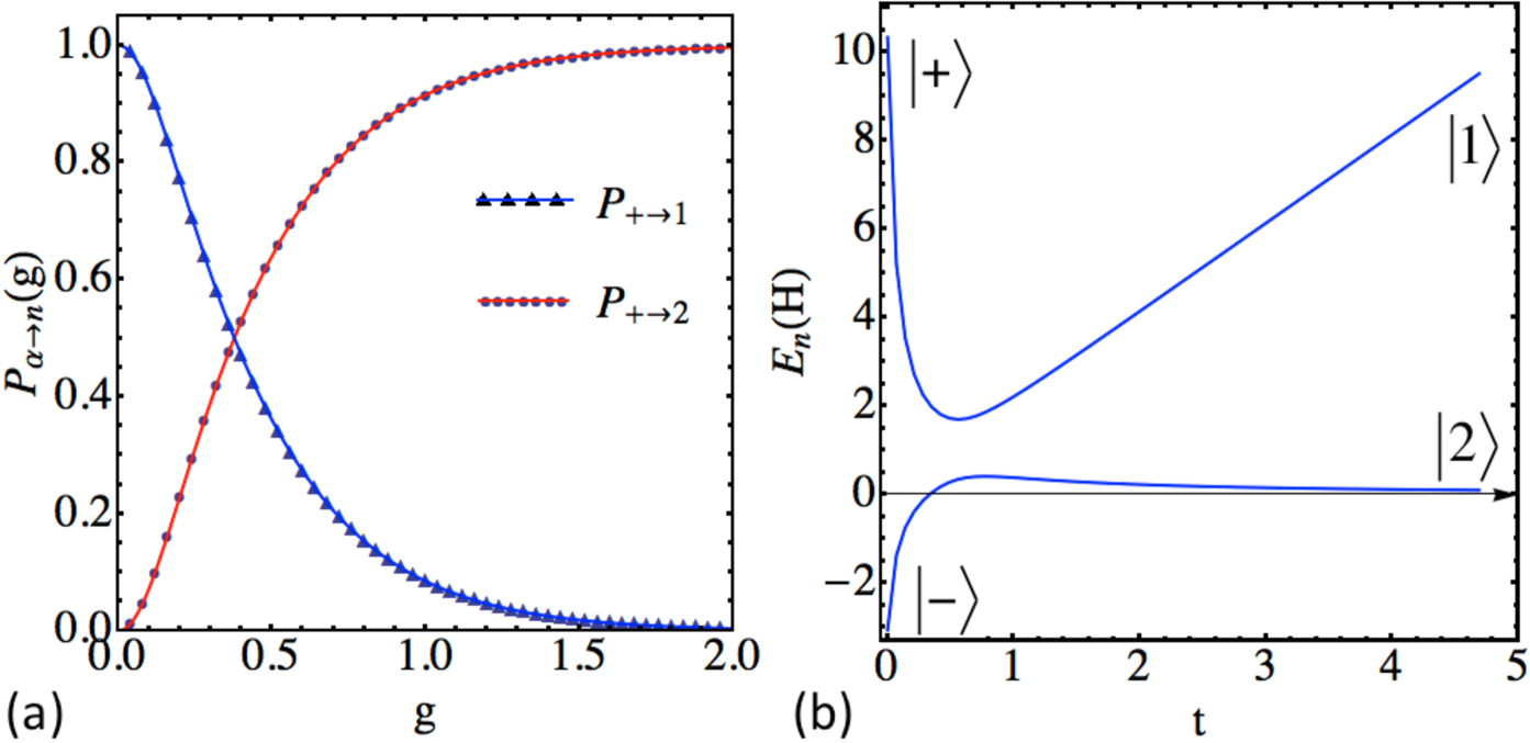
Figure 3: (a) Numerical test of Eq. (38). Solid curves are theoretical predictions and discrete points are numerical results. Parameters: $\beta=2$, $k=0.5$. Solution of Eq. (1) was obtained for the time interval $t\in(0.001,1000)$ with initial condition $|\psi\rangle=|+\rangle$. Details of the numerical program are discussed in supplementary file for Ref. sinitsyn-13prl . (b) Plot of eigenvalues of the Hamiltonian for the model (32) as functions of time at $g=0.4$. At $t\rightarrow 0$, eigenstates coincide with states $|\pm\rangle$, while at $t\rightarrow+\infty$, eigenstatates approach the diabatic states $|1\rangle$ and $|2\rangle$.

Scattering amplitudes from states $|\pm\rangle$ and diabatic states are then well defined for evolution during $t\in(0_{+},+\infty)$. Let $\hat{S}_{+}$ be such a scattering matrix with elements $s_{j\alpha}$, where $j=1,2$ and $\alpha=+,-$. In combination with symmetry (i), the connection formula for the diabatic state $|1\rangle$, i.e. for the state that has the highest slope $\beta>0$, reads:

$$\left(\hat{S}_{+}\hat{S}_{0}^{\rm up}\hat{S}^{\dagger}_{+}\right)_{11}=1,$$ (36)

which can be written in terms of transition probabilities, $p_{\alpha\rightarrow j}\equiv|s_{j\alpha}|^{2}$, as

$$e^{-\pi E_{+}}p_{+\rightarrow 1}+e^{-\pi E_{-}}p_{-\rightarrow 1}=1.$$ (37)

Using the unitarity constraint, $p_{+\rightarrow 2}+p_{-\rightarrow 2}=1$, we finally find:

$$p_{+\rightarrow 1} = p_{-\rightarrow 2}=\frac{e^{-\pi E_{-}}-1}{e^{-\pi E_{-}}-e^{-\pi E_{+}}},$$ (38)

$$p_{-\rightarrow 1} = p_{+\rightarrow 2}=\frac{1-e^{-\pi E_{+}}}{e^{-\pi E_{-}}-e^{-\pi E_{+}}}.$$ (39)

In appendix B, we solve a multistate model that includes result (38) at $k=0$ as a special case. In Fig. 3, we verify predictions of Eqs. (38) numerically by simulating the evolution (1) with the Hamiltonian (32).

III.3 Case 3: $\hat{B}=0$

Here we will explore two possibilities.

${\bf(I)}$ First, we consider the evolution without diagonal elements of the matrix $\hat{C}$:

$$i\frac{d}{dt}\left(\begin{array}[]{c}a\\ b\end{array}\right)=\left(\begin{array}[]{cc}\epsilon&g/t\\ g/t&-\epsilon\end{array}\right)\left(\begin{array}[]{c}a\\ b\end{array}\right),$$ (40)

where $\epsilon>0$.

Since at $t\rightarrow+\infty$ the off-diagonal terms vanish, diabatic states become eigenstates of the Hamiltonian and one can define the scattering matrix from eigenstates of the corresponding matrix $\hat{C}$,

$$|\pm\rangle=\frac{|1\rangle\pm|2\rangle}{\sqrt{2}},$$

to the diabatic states.

The model (40) has interesting property: since the matrix $\hat{B}$ is zero, all diabatic states can be considered as having both the highest and the lowest slope. Moreover, in addition to the previously used connection rules (20)-(21) we have also the option to use the no-go rule (22). Equation (40) is also symmetric under two, simultaneously applied, discrete operations: time reversal $t\rightarrow-t$ and a new discrete operation:

(iv) exchange of indexes: $1\rightarrow 2$, $2\rightarrow 1$. Consider the evolution matrix during time $t\in(0_{+},+\infty)$ from states $|\pm\rangle$ to diabatic states $|1\rangle$, $|2\rangle$:

$$\hat{S}_{+}=\left(\begin{array}[]{cc}s_{1+}&s_{1-}\\ s_{2+}&s_{2-}\end{array}\right).$$ (41)

Under the symmetry (iv), state $|-\rangle$ changes sign and states $|1\rangle$ and $|2\rangle$ transfer into each other. Combining this fact with symmetry operations (i) and (iii), which were defined for previous models, we find the expression for the evolution matrix in negative times in terms of elements $s_{j\alpha}$:

$$\hat{S}_{-}=\left(\begin{array}[]{cc}s_{2+}^{*}&s_{1+}^{*}\\ -s_{2-}^{*}&-s_{1-}^{*}\end{array}\right).$$ (42)

Finally, in the basis $|\pm\rangle$ we have:

$$\hat{S}_{0}^{\rm up}=\left(\begin{array}[]{cc}e^{-\pi g}&0\\ 0&e^{\pi g}\end{array}\right).$$ (43)

For evolution in the upper complex half-plane, it will be easiest to use the no-go rule (22) that reads:

$$\left(\hat{S}_{+}\hat{S}_{0}^{\rm up}\hat{S}_{-}\right)_{12}=0,$$ (44)

or explicity:

$$|s_{1+}|^{2}e^{-\pi g}-|s_{1-}|^{2}e^{\pi g}=0.$$

Combining this with the definition of transition probabilities and the unitarity constraint (i.e. that the matrix of transition probabilities is doubly stochastic), we finally obtain:

$$p_{+\rightarrow 2} = p_{-\rightarrow 1}=\frac{1}{1+e^{2\pi g}},$$ (45)

$$p_{-\rightarrow 2} = p_{+\rightarrow 1}=\frac{1}{1+e^{-2\pi g}}.$$ (46)

${\bf(II)}$ Next, we consider the most general case of evolution with zero matrix $\hat{B}$:

$$i\frac{d}{dt}\left(\begin{array}[]{c}a\\ b\end{array}\right)=\left(\begin{array}[]{cc}\epsilon+k/t&g/t\\ g/t&-\epsilon\end{array}\right)\left(\begin{array}[]{c}a\\ b\end{array}\right),$$ (47)

where $\epsilon>0$. In such a case, there is no obvious symmetry that connects evolution at negative and positive times. However, the number of constraints that we can use includes two constraints (20)-(21) that can be applied to each diabatic level. The latter is because each level can be considered having both the highest and the lowest slope in this model. In addition, there are two no-go constraints (22) depending on whether we choose the contour ${\bm{C}}$ in the upper or the lower half-plane. It turns out, that not all of those constraints are independent of each other but their number is sufficient to estimate transition probabilities, both for negative and positive time evolution.

As in Case 2, we will explore transition probabilities from states $|\pm\rangle$ that are eigenstates of the matrix $\hat{C}$, with eigenvalues $E_{\pm}$ defined in (33), to the diabatic states.

To derive transition probabilities, we will use the fact that any $2\times 2$ unitary matrix can be parametrized by three parameters, $p_{1}$, $\phi_{1}$ and $\theta_{1}$ as follows:

$$\hat{S}_{+}=\left(\begin{array}[]{cc}\sqrt{p_{1}}e^{i\phi_{1}}&\sqrt{1-p_{1}}e^{i\theta_{1}}\\ -\sqrt{1-p_{1}}e^{-i\theta_{1}}&\sqrt{p_{1}}e^{-i\phi_{1}}\end{array}\right).$$ (48)

Similarly, we can parametrize scattering matrix for negative in time evolution:

$$\hat{S}_{-}=\left(\begin{array}[]{cc}\sqrt{p_{2}}e^{i\phi_{2}}&\sqrt{1-p_{2}}e^{i\theta_{2}}\\ -\sqrt{1-p_{2}}e^{-i\theta_{2}}&\sqrt{p_{2}}e^{-i\phi_{2}}\end{array}\right),$$ (49)

and the evolution around $t=0$ is given by

$$\hat{S}_{0}^{\rm up/dn}=\left(\begin{array}[]{cc}e^{\mp\pi E_{+}}&0\\ 0&e^{\mp\pi E_{-}}\end{array}\right).$$ (50)

The no-go rule applied to the contour in the upper half-plane gives

$$\left(\hat{S}_{+}\hat{S}_{0}^{\rm up}\hat{S}_{-}\right)_{12}=0,$$ (51)

which in terms of the introduced parametrization reads:

$$e^{-\pi E_{-}}\sqrt{p_{2}(1-p_{1})}e^{-i(\phi_{2}-\theta_{1})}+$$

$$+e^{-\pi E_{+}}\sqrt{p_{1}(1-p_{2})}e^{i(\phi_{1}+\theta_{2})}=0.$$ (52)

Moving one of the terms in (52) to the rhs and comparing absolute values, we obtain the relation between probabilities:

$$p_{1}(1-p_{2})e^{-2\pi E_{+}}=p_{2}(1-p_{1})E^{-2\pi E_{-}}.$$ (53)

Another equation for probabilities is obtained by applying connection formulas (20)-(21) to the 2nd diabatic state. Subtracting results for the upper and the lower contours from each other we find

$$\left(\hat{S}_{+}\left[\hat{S}_{0}^{\rm up}-\hat{S}_{0}^{\rm dn}\right]\hat{S}_{-}\right)_{22}=0,$$ (54)

which leads to

$$(1-p_{1})(1-p_{2})\left(e^{\pi E_{+}}-e^{-\pi E_{+}}\right)^{2}=p_{1}p_{2}\left(e^{\pi E_{-}}-e^{-\pi E_{-}}\right)^{2}.$$ (55)

Solving (53), and (55) we find:

$$p_{2}=\frac{e^{2\pi E_{-}}(e^{2\pi E_{+}}-1)}{e^{2\pi E_{+}}-e^{2\pi E_{-}}},$$ (56)

$$p_{1}=\frac{e^{2\pi E_{+}}-1}{e^{2\pi E_{+}}-e^{2\pi E_{-}}}.$$ (57)

Note that $p_{1}\neq p_{2}$, i.e. we were able to find nontrivial transition probabilities simultaneously for the negative and the positive evolution time intervals. Finally, with unitarity constraints, we can identify transition probabilities for positive time:

$$p_{+\rightarrow 1}=p_{-\rightarrow 2}=p_{1},\quad p_{+\rightarrow 2}=p_{-\rightarrow 1}=1-p_{1}.$$ (58)

This example shows that it is not always necessary to use discrete symmetries in order to obtain interesting results with connection formulas.

IV Multistate LZC systems

The two-state systems that were solved analytically in previous section can, in principle, be solved by other means. For example, all of them can be reduced to the well-understood confluent hypergeometric equation. In contrast, much less is known about how to solve systems with $N>2$. Therefore, this section contains most important results that demonstrate how connection formulas can make a nontrivial insight in the behavior of transition probabilities in multistate models.

IV.1 Special State Model

Consider a model in which arbitrary number $N$ of states interact with a single special state, to which we will give zero index, and

(i) matrix $\hat{B}$ is not degenerate;

(ii) matrix $\hat{A}$ contains nonzero elements only as couplings of the special state to the other states, i.e. $A_{i0}=A_{0i}=g_{i}$ and all other elements of $\hat{A}$ are zero;

(iii) matrix $\hat{C}$ has arbitrary nonzero elements except couplings to the special state, i.e. $C_{i0}=C_{0i}=0$.

The Hamiltonian of such a system in the diabatic basis has the form:

$$\hat{H}(t)=\left(\begin{array}[]{ccccc}k_{0}/t&g_{1}&g_{2}&\ldots&g_{N}\\ g_{1}&\beta_{1}t+k_{1}/t&g_{12}/t&\ldots&g_{1N}/t\\ g_{2}&g_{12}/t&\beta_{2}t+k_{2}/t&\ldots&\ldots\\ \vdots&\vdots&\vdots&\ddots&\vdots\end{array}\right).$$ (59)

Let $s_{j\alpha}$, where $\alpha,j\in(0,\ldots N)$, be the transition amplitude from the $\alpha$-th eigenstate of $\hat{C}$ to the $j$-th diabatic state for positive in time evolution from $t\rightarrow 0_{+}$ to $t\rightarrow+\infty$, i.e.

$$\hat{S}_{+}=\left(\begin{array}[]{cccc}s_{00}&s_{01}&\ldots&s_{0N}\\ s_{10}&s_{11}&\ldots&\vdots\\ \vdots&\vdots&\ddots&\vdots\end{array}\right).$$ (60)

Evolution equation (1) with the Hamiltonian (59) is symmetric under the time reflection, $t\rightarrow-t$, followed by the change of the sign of the amplitude of the special state. In turn, this means that the scattering matrix for the evolution from $t\rightarrow-\infty$ to $t\rightarrow 0_{-}$ has the form:

$$\hat{S}_{-}=\left(\begin{array}[]{ccccc}s^{*}_{00}&-s^{*}_{10}&\ldots&\ldots&-s^{*}_{N0}\\ -s_{01}^{*}&s^{*}_{11}&s^{*}_{21}&\ldots&\vdots\\ -s_{02}^{*}&s^{*}_{12}&s^{*}_{22}&\ldots&\vdots\\ \vdots&\vdots&\vdots&\ddots&\vdots\end{array}\right).$$ (61)

Suppose, first, that the state $|0\rangle$ has the highest/lowest slope. Then in the basis of eigenstates of $\hat{C}$, we have: $\hat{S}_{0}^{\rm up}={\rm diag}\{e^{\mp\pi k_{0}},e^{\mp\pi E_{1}},\ldots e^{\mp\pi E_{N}}\}$, where $E_{i}$ are eigenvalues of the matrix $\hat{C}$, and the choice of $-/+$ depends on whether the state has the highest/lowest slope, which in turn determines whether the contour ${\bm{C}_{0}}$ should be in the upper or in the lower complex half-plane. Substituting this and (60)-(61) into (20)-(21) we obtain:

$$e^{\mp\pi k_{0}}p_{0\rightarrow 0}-\sum_{i=1}^{N}e^{\mp\pi E_{i}}p_{i\rightarrow 0}=e^{\pi(\mp k_{0}-\sum_{i=1}^{N}g_{i}^{2}/|\beta_{i}|)}.$$ (62)

If, instead, a level with $n\neq 0$ has the highest/lowest slope, then (20)-(21) lead to the constraint:

$$-e^{\mp\pi k_{0}}p_{0\rightarrow n}+\sum_{i=1}^{N}e^{\mp\pi E_{i}}p_{i\rightarrow n}=e^{\pi(\mp k_{n}-g_{n}^{2}/|\beta_{n}|)}.$$ (63)

Although Eqs. (62)-(63) do not determine a particular element of the transition probability matrix, they represent exact nonperturbative constraints that reduce the number of unknown independent parameters of the transition probability matrix. In special cases these equations can be used to derive specific probabilities. Consider, e.g., the situation in which only one element of the matrix $\hat{C}$ is nonzero, i.e. $C_{00}=k_{0}$. In such a case, $E_{i}=0$ for $i=1,\ldots N$. Using the unitarity condition, $\sum_{i=0}^{N}p_{i\rightarrow 0}=1$, Eqs. (62)-(63) tell that if the level $0$ is extremal then

$$p_{0\rightarrow 0}=\frac{1+e^{\pi(\mp k_{0}-\sum_{i=1}^{N}g_{i}^{2}/|\beta_{i}|)}}{1+e^{\mp\pi k_{0}}},$$ (64)

and if a level with $n\neq 0$ is extremal then

$$p_{0\rightarrow n}=\frac{1-e^{-\pi g_{n}^{2}/|\beta_{n}|}}{1+e^{\mp\pi k_{0}}},$$ (65)

where $-/+$ corresponds to the situation in which a given level has the highest/lowest slope. Probabilities (64)-(65) coincide with their values known from the exact solution of this model sinitsyn-13prl .

IV.2 Model with two special states

Consider now a generalization of the previous model in which two states, with indexes $0$ and $0^{\prime}$, equally interact with other states. Diabatic energies of those states are separated by a finite distance: $A_{00}=-A_{0^{\prime}0^{\prime}}=\epsilon$ and those states are allowed to interact with each other with a decaying coupling: $C_{00^{\prime}}=C_{0^{\prime}0}=g/t$. The Hamiltonian of this system can be written in the following matrix form:

$$\hat{H}(t)=\left(\begin{array}[]{ccccc}\epsilon&g/t&g_{1}&\ldots&g_{N}\\ g/t&-\epsilon&g_{1}&\ldots&g_{N}\\ g_{1}&g_{1}&\beta_{1}t+k_{1}/t&g_{12}/t&\ldots\\ g_{2}&g_{2}&g_{12}/t&\beta_{2}t+k_{2}/t&\ldots\\ \vdots&\vdots&\vdots&\ddots&\vdots\end{array}\right).$$ (66)

Matrix $\hat{C}$ has two eigenvectors that can be written explicitly:

$$|\pm\rangle=\frac{1}{\sqrt{2}}\left(|0\rangle\pm|0^{\prime}\rangle\right),$$ (67)

with eigenvalues $E_{\pm}=\pm g$. For other eigenvalues of $\hat{C}$ we will use notation of the previous model. For example, $\hat{S}_{0}^{\rm up/dn}={\rm diag}\{e^{\mp\pi E_{+}},e^{\mp\pi E_{-}},e^{\mp\pi E_{1}},\ldots e^{\mp\pi E_{N}}\}$.

Evolution equation (1) with the Hamiltonian (66) is symmetric under simultaneous time reversal, change of sign of special state amplitudes, and exchange of their indexes: $0\rightarrow 0^{\prime}$ and $0^{\prime}\rightarrow 0$. The latter operation leaves the state $|+\rangle$ invariant and changes the sign of $|-\rangle$. Consequently, if the scattering matrix for positive time has the form

$$\hat{S}_{+}=\left(\begin{array}[]{ccccc}s_{0+}&s_{0-}&s_{01}&\ldots&s_{0N}\\ s_{0^{\prime}+}&s_{0^{\prime}-}&s_{0^{\prime}1}&\ldots&\vdots\\ s_{1+}&s_{1-}&s_{11}&\ldots&\vdots\\ \vdots&\vdots&\ldots&\ddots&\vdots\end{array}\right),$$ (68)

then the scattering matrix for the negative time evolution has the form:

$$\hat{S}_{-}=\left(\begin{array}[]{ccccc}s_{0^{\prime}+}^{*}&s^{*}_{0+}&-s_{1+}^{*}&\ldots&-s_{N+}^{*}\\ -s_{0^{\prime}-}^{*}&-s_{0-}^{*}&s_{1-}^{*}&\ldots&\vdots\\ -s_{0^{\prime}1}^{*}&-s_{01}^{*}&s_{11}^{*}&\ldots&\vdots\\ \vdots&\vdots&\ldots&\ddots&\vdots\end{array}\right).$$ (69)

Suppose that the special levels have the highest slope. Then the transition from the state $|0^{\prime}\rangle$ to the state $|0\rangle$ is counterintuitive. The No-Go Rule then produces a simple relation for transition probabilities:

$$e^{-\pi g}p_{+\rightarrow 0}-e^{\pi g}p_{-\rightarrow 0}-\sum_{i=1}^{N}e^{-\pi E_{i}}p_{i\rightarrow 0}=0.$$ (70)

If, in this situation, the level with index $n\neq\{0,0^{\prime}\}$ has the lowest slope then the connection rule (21) gives:

$$-e^{\pi g}p_{+\rightarrow n}+e^{-\pi g}p_{-\rightarrow n}+\sum_{i=1}^{N}e^{\pi E_{i}}p_{i\rightarrow n}=e^{\pi(k_{n}-2g_{n}^{2}/|\beta_{n}|)}.$$ (71)

For example, consider a special case: $C_{ii}=-g$ and $C_{ij}=0$, for $i,j=1,\ldots N$. In such a case, $E_{i}=k_{i}=-g$, and after using the doubly stochastic character of the transition probability matrix, Eqs. (70)-(71) produce simple results:

$$p_{+\rightarrow 0}=\frac{1}{1+e^{-2\pi g}},\quad p_{+\rightarrow n}=\frac{1-e^{-2\pi g_{n}^{2}/|\beta_{n}|}}{1+e^{2\pi g}}.$$ (72)

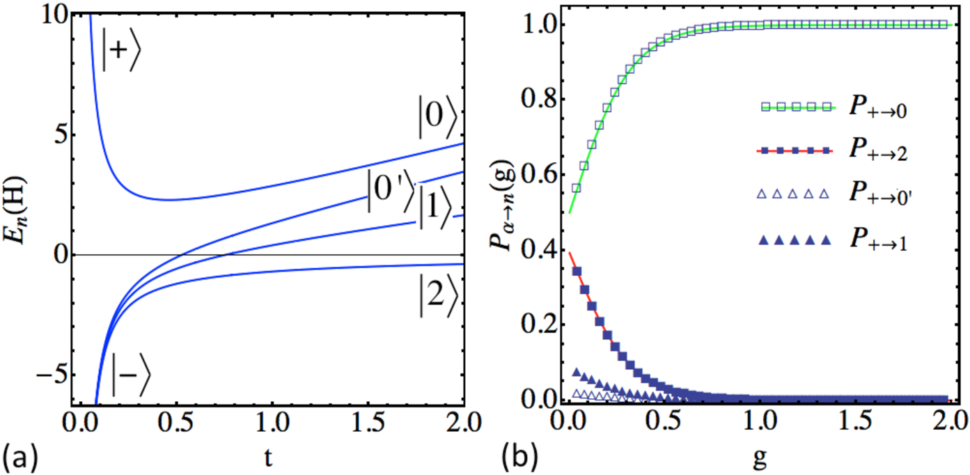
Figure 4: (a) Plot of eigenvalues of the Hamiltonian (73). (b) Numerical test of Eq. (72). Parameters for numerical simulations: $g_{1}=0.5$, $g_{2}=0.7$, $\epsilon=0.5$. Evolution time interval is $t\in(0.001,1000)$. Solid curves are theoretical predictions and discrete points are numerical results.

For a numerical check, we consider the latter model with $N=4$ and the Hamiltonian

$$\hat{H}=\left(\begin{array}[]{cccc}\epsilon+2t&g/t&g_{1}&g_{2}\\ g/t&-\epsilon+2t&g_{1}&g_{2}\\ g_{1}&g_{1}&t-g/t&0\\ g_{2}&g_{2}&0&-g/t\end{array}\right).$$ (73)

In Fig. 4, we illustrate eigenvalues of this Hamiltonain as functions of $t$ and compare Eq. (72) with results of numerical simulations, which are found to be in perfect agreement with each other.

IV.3 Chain models

There are numerous physical applications, in which diabatic states are coupled by a constant coupling in a chain-like fashion with all other elements of matrix $\hat{A}$ being zero chain1 . In such a case, Eq. (1) transforms into the set of coupled equations:

$$i\dot{\psi}_{n}=(k_{n}/t+\beta_{n}t)\psi_{n}+g_{n}\psi_{n+1}+g_{n-1}\psi_{n-1},$$ (74)

where $n=1,\ldots,N$, and where we define $g_{0}=g_{N}=0$. For evolution (74), diabatic states coincide with eigenstates both at $t\rightarrow 0$ and at $t\rightarrow\infty$. Equation (74) is symmetric under simultaneous time reversal $t\rightarrow-t$ and the change of the sign of the amplitudes with even indexes. Therefore, the scattering matrix for negative time is written in terms of matrix elements $s_{ij}$, $i,j=1,\ldots,N$, for positive time as

$$\hat{S}_{-}=\left(\begin{array}[]{cccc}s_{11}^{*}&-s^{*}_{21}&s_{31}^{*}&\ldots\\ -s_{12}^{*}&s_{22}^{*}&-s_{32}^{*}&\vdots\\ s_{13}^{*}&-s_{23}^{*}&s_{33}^{*}&\vdots\\ \vdots&\vdots&\ldots&\ddots\end{array}\right),$$ (75)

Consider the case when a state with index $n$ has the highest/lowest slope. Then if $n$ is odd, Eqs. (20)-(21) return:

$$\sum_{i=1}^{N}(-1)^{i+1}p_{i\rightarrow n}e^{\mp\pi k_{i}}=e^{-\pi\left(\pm k_{n}+\frac{g_{n}^{2}}{|\beta_{n}-\beta_{n+1}|}+\frac{g_{n-1}^{2}}{|\beta_{n}-\beta_{n-1}|}\right)}.$$ (76)

If $n$ is even then

$$\sum_{i=1}^{N}(-1)^{i}p_{i\rightarrow n}e^{\mp\pi k_{i}}=e^{-\pi\left(\pm k_{n}+\frac{g_{n}^{2}}{|\beta_{n}-\beta_{n+1}|}+\frac{g_{n-1}^{2}}{|\beta_{n}-\beta_{n-1}|}\right)},$$ (77)

where $-/+$ corresponds to the highest/lowest slope of the extremal level.

Here we note also that the same symmetry and, hence, the form of the scattering matrix (75) is obtained if we generalize the chain model to include (a) constant couplings between states with arbitrary even and odd indexes and (b) decaying with time couplings between states of the same index parity. Equasions (76)-(77) are straightforward to generalize to these situations.

IV.4 Models with $\hat{A}=0$

Equation (1), in the case of $\hat{A}=0$, arbitrary $\hat{C}$, and non-degenerate $\hat{B}$, is symmetric under reflection $t\rightarrow-t$. Let $E_{\alpha}$, $\alpha=1,\ldots,N$ be the eigenvalues of the matrix $\hat{C}$. Then for the extremal state with index $n$, (20) gives:

$$\sum_{\alpha=1}^{N}e^{\mp\pi E_{\alpha}}p_{\alpha\rightarrow n}=e^{\mp\pi k_{n}},$$ (78)

where $+/-$ corresponds to the highest/lowest slope.

As an example, consider the case when all levels are coupled to each other according to the rule

$$C_{ij}=q_{i}q_{j},\quad i,j=1,\ldots,N,$$ (79)

with $N$ independent constants $q_{i}$. In such a case, matrix $\hat{C}$ has all zero eigenvalues except the one that corresponds to the state vector

$$|+\rangle=\frac{1}{\sqrt{E_{+}}}\left(q_{1}|1\rangle+\ldots+q_{N}|N\rangle\right),$$ (80)

with a single nonzero eigenvalue $E_{+}=\sum_{i=1}^{N}q_{i}^{2}$. Note also that $k_{n}=q_{n}^{2}$. Substituting this into (78) and using the unitarity condition we find

$$p_{+\rightarrow n}=\frac{1-e^{\mp\pi q_{n}^{2}}}{1-e^{\mp\pi\sum_{i=1}^{N}q_{i}^{2}}}.$$ (81)

In Appendix B, we show that, for the latter model, one can derive explicit expressions for transition probabilities from the state $|+\rangle$ to any other state by an alternative approach. The final result is in perfect agreement with (81).

IV.5 Models with $\hat{B}=0$

Here we will explore two specific 3-state systems.

IV.5.1 Case-1: Equal Coupling Model

Consider a 3-state model with the Hamiltonian

$$\hat{H}(t)=\left(\begin{array}[]{ccc}\epsilon&g/t&g/t\\ g/t&0&g/t\\ g/t&g/t&-\epsilon\end{array}\right),$$ (82)

which eigenvalues as functions of time are shown in Fig. 5(a). Matrix $\hat{C}$ has an eigenvalue $E_{+}=2g$ with an eigenvector

$$|+\rangle=\frac{1}{\sqrt{3}}\left(|1\rangle+|2\rangle+|3\rangle\right),$$ (83)

and two degenerate eigenvalues $E_{0}=E_{0^{\prime}}=-g$ with eigenvectors

$$|0\rangle=\frac{|1\rangle-|3\rangle}{\sqrt{2}},\quad|0^{\prime}\rangle=\frac{|1\rangle-2|2\rangle+|3\rangle}{\sqrt{6}}.$$ (84)

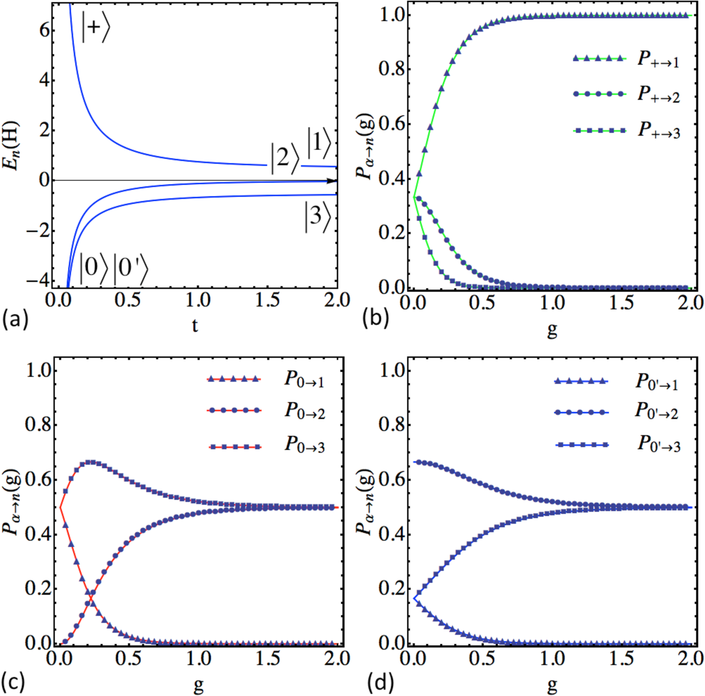
Figure 5: (a) Plot of eigenvalues of the Hamiltonian (82) as functions of time at $g=0.3$, $\epsilon=0.5$. (b-d) Numerical test of Eqs. (91), (96) at $\epsilon=0.5$ for different couplings $g$. Evolution time interval is $t\in(0.001,1000)$. Solid curves are theoretical predictions and discrete points are results of the numerical solution of the evolution equation with the Hamiltonian (82).

Equation (1) with the Hamiltonian (82) is symmetric under the time reversal and, simultaneously, exchange of indexes $1\rightarrow 3$ and $3\rightarrow 1$. Note that the index exchange leaves states $|+\rangle$ and $|0^{\prime}\rangle$ invariant but changes the sign of $|0\rangle$.

Let the scattering matrix for the positive time evolution have the form

$$\hat{S}_{+}=\left(\begin{array}[]{ccc}s_{1+}&s_{10}&s_{10^{\prime}}\\ s_{2+}&s_{20}&s_{20^{\prime}}\\ s_{3+}&s_{30}&s_{30^{\prime}}\end{array}\right),$$ (85)

then the negative time scattering matrix reads:

$$\hat{S}_{-}=\left(\begin{array}[]{ccc}s_{3+}^{*}&s_{2+}^{*}&s_{1+}^{*}\\ -s_{30}^{*}&-s_{20}^{*}&-s_{10}^{*}\\ s_{30^{\prime}}^{*}&s_{20^{\prime}}^{*}&s_{10^{\prime}}^{*}\end{array}\right),$$ (86)

and in the basis of states (83)-(84)

$$\hat{S}_{0}^{\rm up/dn}={\rm diag}\{e^{\mp\pi E_{+}},e^{\mp\pi E_{0}},e^{\mp\pi E_{0^{\prime}}}\}.$$ (87)

Here we note again that the case with $\hat{B}=0$ is, in some sense, unusual: all its states can be simultaneously considered as having both the highest and the lowest slope and all off-diagonal transitions can be considered counterintuitive, although depending on whether levels are considered having the highest or the lowest slope. Applying the No-Go Rule to transitions between levels $3$ and $1$, we find constraints on probabilities:

$$p_{+\rightarrow 1}e^{-2\pi g}-p_{0\rightarrow 1}e^{\pi g}+p_{0^{\prime}\rightarrow 1}e^{\pi g}=0,$$ (88)

$$p_{+\rightarrow 3}e^{2\pi g}-p_{0\rightarrow 3}e^{-\pi g}+p_{0^{\prime}\rightarrow 3}e^{-\pi g}=0,$$ (89)

and applying the connection formulas (20)-(21) to the state $|2\rangle$ we find

$$p_{+\rightarrow 2}e^{\pm 2\pi g}-p_{0\rightarrow 2}e^{\mp\pi g}+p_{0^{\prime}\rightarrow 2}e^{\mp\pi g}=1.$$ (90)

In combination with the unitarity rule: $p_{+\rightarrow 2}+p_{0\rightarrow 2}+p_{0^{\prime}\rightarrow 2}=1$, Eq. (90) leads to explicit expressions for transitions to the 2nd state:

$$p_{+\rightarrow 2}=\frac{1}{1+2\cosh(2\pi g)},\quad p_{0\rightarrow 2}=\frac{\cosh(\pi g)-1}{2\cosh(\pi g)-1},\quad p_{0^{\prime}\rightarrow 2}=\frac{\cosh(\pi g)+1}{2\cosh(\pi g)+1}.$$ (91)

At a first view, it seems that rules (88)-(89) are insufficient to determine the remaining unknown elements of the transition probability matrix, while the interpretation of the unused constraints in terms of the probabilities seems obscure. However, below, we will show that the model with $\hat{B}=0$ contains one extra useful property that, in our case, produces new simple constraints on transition probabilities.

IV.5.2 Duality between $\hat{B}=0$ and $\hat{A}=0$ models

Consider arbitrary model (1) with $\hat{A}=0$:

$$i\frac{d\psi}{dt}=\left(\hat{B}t+\frac{\hat{C}}{t}\right)\psi.$$ (92)

For strictly positive time, $t>0$, we can make a change of variables: $t^{2}/2=\tau$. Transition from $t$ to $\tau$ does not change the scattering matrix for evolution during $t\in(0_{+},+\infty)$. Using that $d/dt=td/d\tau$, we then find:

$$i\frac{d\psi}{d\tau}=\left(\hat{B}+\frac{\hat{C}}{2\tau}\right)\psi,$$ (93)

i.e. the change of variables that does not affect transition probability matrix for $t>0$ transforms the model with ($\hat{A}=0$) into the model with ($\hat{B}=0$) but with elements of the matrix $\hat{C}$ rescaled by a factor $1/2$.

This means that we can apply Eq. (78) to the levels having the extremal (largest or lowest) value of the parameter $\epsilon_{i}$ in any model of the $\hat{B}=0$ type. In particular, application of this rule to the extremal levels of the model (82) gives:

$$e^{-4\pi g}p_{+\rightarrow 1}+e^{2\pi g}p_{0\rightarrow 1}+e^{2\pi g}p_{0^{\prime}\rightarrow 1}=1,$$ (94)

$$e^{4\pi g}p_{+\rightarrow 3}+e^{-2\pi g}p_{0\rightarrow 3}+e^{-2\pi g}p_{0^{\prime}\rightarrow 3}=1.$$ (95)

In fact, one of expressions (94)-(95) is redundant, as only one of them is sufficient to reconstruct all remaining transition probabilities:

$$p_{+\rightarrow 1} = \frac{e^{4\pi g}}{1+e^{2\pi g}+e^{4\pi g}},\quad p_{0\rightarrow 1}=\frac{1}{2-2e^{\pi g}+2e^{2\pi g}},\quad p_{0^{\prime}\rightarrow 1}=\frac{1}{2(1+e^{\pi g}+e^{2\pi g})},$$

$$\quad p_{+\rightarrow 3} = \frac{1}{1+e^{2\pi g}+e^{4\pi g}},\quad p_{0\rightarrow 3}=\frac{e^{\pi g}}{4\cosh(\pi g)-2},\quad\,\,\,p_{0^{\prime}\rightarrow 3}=\frac{e^{\pi g}}{4\cosh(\pi g)+2}.$$ (96)

In Fig. 5(b-d) we provide numerical test of (91) and (96) that shows perfect agreement of theory and numerics.

IV.5.3 Case-2: Chain model with decaying couplings

Consider another example of a 3-state model with the Hamiltonian

$$\hat{H}(t)=\left(\begin{array}[]{ccc}\epsilon&g/t&0\\ g/t&k/t&g/t\\ 0&g/t&-\epsilon\end{array}\right),$$ (97)

which eigenvalues, as functions of $t$, are shown in Fig. 6(a). Corresponding matrix $\hat{C}$ has one eigenstate

$$|0\rangle=\frac{1}{\sqrt{2}}\left(|1\rangle-|3\rangle\right)$$ (98)

that corresponds to the zero eigenvalue, and two eigenstates, $|+\rangle$ and $|-\rangle$, that correspond to eigenvalues

$$E_{\pm}=\frac{1}{2}\left(k\pm\sqrt{k^{2}+8g^{2}}\right).$$ (99)

One can check that under exchange of indexes $1\rightarrow 3$ and $3\rightarrow 1$, eigenstate $|0\rangle$ changes sign, while eigenstates $|\pm\rangle$ remain invariant. The No-Go Rule then produces constraints:

$$p_{+\rightarrow 1}e^{-\pi E_{+}}-p_{0\rightarrow 1}+p_{-\rightarrow 1}e^{-\pi E_{-}}=0,$$ (100)

$$p_{+\rightarrow 3}e^{\pi E_{+}}-p_{0\rightarrow 3}+p_{-\rightarrow 3}e^{\pi E_{-}}=0.$$ (101)

The connection formulas (20)-(22) applied to the diabatic state $|2\rangle$ produces

$$p_{+\rightarrow 2}e^{\mp\pi E_{+}}-p_{0\rightarrow 2}+p_{-\rightarrow 2}e^{\mp\pi E_{-}}=e^{\mp\pi k},$$ (102)

and the duality produces an additional constraint:

$$p_{+\rightarrow 1}e^{-2\pi E_{+}}+p_{0\rightarrow 1}+p_{-\rightarrow 1}e^{-2\pi E_{-}}=1.$$ (103)

Altogether, Eqs. (100)-(103) and the doubly stochastic character of the transition probability matrix produce the set of transition probabilities:

$$p_{+\rightarrow 2} = \frac{e^{-\pi E_{-}}(1+e^{\pi k})(e^{\pi k}-e^{\pi E_{-}})}{(1+e^{\pi E_{+}})(e^{\pi E_{+}}-e^{\pi E_{-}})},\quad p_{0\rightarrow 2}=\frac{e^{\pi E_{+}}+e^{\pi E_{-}}-1-e^{\pi k}}{1+e^{\pi E_{+}}+e^{\pi E_{-}}+e^{\pi k}},\quad p_{-\rightarrow 2}=\frac{e^{-\pi E_{+}}(1+e^{\pi k})(e^{\pi E_{+}}-e^{\pi k})}{(1+e^{\pi E_{-}})(e^{\pi E_{+}}-e^{\pi E_{-}})},\quad$$ (104)

$$\quad\quad\quad\quad p_{-\rightarrow 3}=e^{-2\pi E_{-}}p_{-\rightarrow 1},\quad\quad p_{+\rightarrow 3}=e^{-2\pi E_{+}}p_{+\rightarrow 1},$$

$$p_{+\rightarrow 1} = \frac{e^{2\pi E_{+}}(1-e^{\pi E_{-}})}{(e^{\pi E_{+}}+1)(e^{\pi E_{+}}-e^{\pi E_{-}})},\quad p_{-\rightarrow 1}=\frac{e^{2\pi E_{-}}(e^{\pi E_{+}}-1)}{(e^{\pi E_{-}}+1)(e^{\pi E_{+}}-e^{\pi E_{-}})},\quad p_{0\rightarrow 1}=p_{0\rightarrow 3}=\frac{1+e^{\pi k}}{1+e^{\pi E_{+}}+e^{\pi E_{-}}+e^{\pi k}}.$$

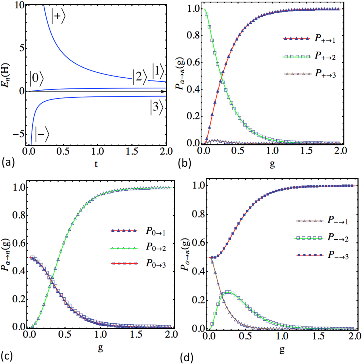
Figure 6: (a) Plot of eigenvalues of the Hamiltonian (97) as functions of time at $g=\epsilon=0.5$, $k=2$. (b-d) Numerical test of Eqs. (104) at $\epsilon=0.5$, $k=0.3$ for different couplings $g$. Evolution time interval is $t\in(0.001,1000)$. Solid curves are theoretical predictions and discrete points are results of the numerical solution of the evolution equation with the Hamiltonian (97).

In Fig. 6(b-d) we compare theoretical predictions (104) with transition probabilities obtained with numerical simulations and find perfect agreement between them.

V Discussion and Conclusion

In this work, we demonstrated that the absence of the Stokes phenomenon is the property of solutions in a large class of LZC-systems (1). For any such a model, it is possible to obtain exact nontrivial constraints on the elements of the scattering matrix. Generally, those constraints do not show a simple interpretation in terms of transition probabilities for evolution from $t\rightarrow 0_{+}$ to $t\rightarrow+\infty$. However, there is quite a large subclass of LZC systems that contain additional discrete symmetries that eventually lead to simple linear constraints on elements of the transition probability matrix and, sometimes, even to analytical expressions for probabilities of particular transitions.

Certainly, it is likely that examples found in this article do not exhaust the set of tricks that can be applied to derive new interesting solutions of LZC models. So the future progress in this direction is expected. Here we would like to point to alternative research directions, which have not been explored in the present article.

First, we note that the proof of the absence of the Stokes phenomenon can be applied to even larger class of systems. For example, one can consider the Generalized LZC Model with the Hamiltonian

$$\hat{H}=\hat{A}+\hat{B}t+\sum_{i=0}^{L}\frac{\hat{C}_{i}}{t-t_{i}}$$ (105)

that has similar, to the LZC model, behavior of asymptotic solutions near points $t_{i}$ and $t\rightarrow\infty$. In such a case, a contour at $R\rightarrow\infty$ that connects asymptotics at $t\rightarrow\pm\infty$ can be continuously deformed to lay along the real axis except the points $t_{i}$ that it should encircle. It would be interesting to find out whether it is possible to derive useful constraints on transition probabilities for models of the type (105) by imposing additional symmetries of the Hamiltonian, as we did in the present work for the LZC model.

The second observation that can be useful is that even if only one of the amplitudes is completely known along a contour then all other solutions can be found as integrals of this known amplitude. For example, an arbitrary evolution of a two-state system with time-dependent coefficients can be written in the following form:

$$i\dot{a} = e(t)a+g^{*}(t)b,$$

$$i\dot{b} = g(t)a.$$

Let ${\bm{C}}$ be a contour that goes around the infinite time semicircle connecting $t\rightarrow\pm\infty$ asymptotics at the real axis as we discussed before. If for some reason the amplitude $a(t)$ is known along ${\bm{C}}$ with initial conditions $(a,b)=(1,0)$ at $t\rightarrow-\infty$, then one can also connect asymptotic values for $b(t)$ as

$$b(t\rightarrow+\infty)=-i\int_{\bm{C}}dt^{\prime}g(t^{\prime})a(t^{\prime}).$$ (106)

Applying this idea to the extremal amplitude of an LZC model, one would find, however, that it is not enough to know the leading terms in $1/t$ for the amplitude $a(t)$ along ${\bm{C}}$ because subleading terms in the expansion of $a(t)$ over the small parameter $1/t$ generally produce a finite contribution to (106). Nevertheless, imagine that one can find a formal solution for the amplitude $a(t)$ of an extremal state in an LZC-type model in terms of a formal series in powers of the small parameter $1/t$ along ${\bm{C}}$. One can then directly substitute this formal solution in expressions like (106) and, after evaluating Gaussian integrals over time, obtain the series that determines the asymptotic values of other elements of the evolution matrix. So the problem reduces to the question whether interesting LZC models can be found for which not only leading asymptotics but the whole series in powers of $1/t$ can be written explicitly, i.e. not in terms of recursion relations but rather in terms of explicit expressions for coefficients of this expansion over $1/t$, e.g. in the form of the Tailor series for the generalized hypergeometric function.

The Stokes phenomenon in systems of differential equations with polynomial in time coefficients has been extensively discussed in mathematical literature math . However, mathematical results have been usually formalized to include too general equations that lack a transparent physical interpretation. In contrast, the major goal of exactly solvable models in physics is to obtain the intuition about a complex nonperturbative regime. Hence, valuable formulas must be written in terms of physically measurable characteristics, such as transition probabilities. Usually most interesting exact results can be expressed via elementary functions of model’s parameters. It can be also useful when a solvable model can produce an insight into numerically challenging situations with a macroscopic number of interacting states ($N\gg 1$).

We hope that explicit examples that we provided will raise the interest in quantum mechanical properties of LZC modes, and this article will be used as the bridge between mathematical literature and physically interesting applications.

Appendix A Multistate Landau-Zener models with linear level crossings

Consider the Hamiltonian with linear time dependence of parameters:

$$\hat{H}=\hat{A}+\hat{B}t.$$ (107)

Since the Hamiltonian (107) has no singularity at $t=0$, typically the scattering problem is formulated for the evolution from $t\rightarrow-\infty$ to $t\rightarrow+\infty$, and we will focus on this case here too.

A.1 Brundobler-Elser Formula and No-Go Theorem

It was observed, initially in numerical simulations be , that for any model of the form (107) there are elements of the transition probability matrix, for evolution during $t\in(-\infty,+\infty)$, that can be found by a simple application of the two state Landau-Zener formula at every intersection of diabatic energies. Ref. be presented a formula for the diagonal element of the scattering matrix for the state whose diabatic energy level has the extremal slope, i.e. if $k$ is the index of the state with $B_{kk}=\max(\beta_{1}\ldots\beta_{N})$ or $B_{kk}=\min(\beta_{1}\ldots\beta_{N})$ then

$$|S_{kk}(+\infty,-\infty)|=\exp\left(-\pi\sum\limits_{i\,(i\neq k)}\frac{|A_{ki}|^{2}}{|\beta_{k}-\beta_{i}|}\right).$$ (108)

In no-go another exact result, called the “no-go theorem”, was found in the case when instead of one state with the highest (or one lowest) slope of the diabatic energy level there is a band of an arbitrary number of states having the same highest slope so that diabatic energies in this band are different only by constant energy parameters. The no-go theorem states that the counterintuitive transitions, as they are defined in the main text, are exactly forbidden:

$$P_{n\rightarrow m}\equiv|S_{mn}(-\infty,+\infty,)|=0.$$ (109)

One can easily verify that (108)-(109) are direct consequences of the rules (20)-(22) applied to the systems with the Hamiltonian (107). We note also that validity of (108)-(109) was proved by an alternative approach in mlz-1 .

A.2 Discrete symmetries in systems with linear level crossings

Discrete symmetries of evolution equations with the Hamiltonian (107) can be useful to derive constraints on transition probabilities. Here we will show two examples.

First, consider the class of models of transitions on a linear chain chain with evolution of amplitudes $a_{n}(t)$, $n=1,\ldots,N$, of the form:

$$i\dot{a}_{n}=\beta_{n}ta_{n}+g_{n}a_{n+1}+g_{n-1}a_{n},\quad g_{0}=g_{N}=0.$$ (110)

As we discussed in section IV.C, this system is symmetric under the sign change of time and, simultaneously, the sign change of amplitudes with even indexes. Applying this symmetry to off-diagonal elements of the scattering matrix for evolution from $t\rightarrow-\infty$ to $t\rightarrow+\infty$, we find that $s_{ij}=\pm s_{ji}^{*}$. The latter symmetry means that the transition probability matrix is symmetric:

$$p_{i\rightarrow j}=p_{j\rightarrow i},$$ (111)

which explains some observations in chain .

Second, consider a 3-state model with equal couplings between any pair of states:

$$\hat{H}(t)=\left(\begin{array}[]{ccc}\beta t&g&g\\ g&0&g\\ g&g&-\beta t\end{array}\right).$$ (112)

Exact solution for this model has not been found. However, this model is symmetric under three simultaneously applied operations:

(i) time reversal $t\rightarrow-t$;

(ii) change of indexes, $1\rightarrow 3$ and $3\rightarrow 1$;

(iii) complex conjugation of the evolution equation.

Let the scattering matrix have the form

$$\hat{S}(+\infty|-\infty)=\left(\begin{array}[]{ccc}s_{11}&s_{12}&s_{13}\\ s_{21}&s_{22}&s_{23}\\ s_{31}&s_{32}&s_{33}\end{array}\right),$$ (113)

then applying a sort of CPT symmetry (i)-(iii) in combination with unitarity, $S(t_{1}|t_{2})=S^{\dagger}(t_{2}|t_{1})$, we find that

$$\hat{S}(+\infty|-\infty)=\left(\begin{array}[]{ccc}s_{33}&s_{23}&s_{13}\\ s_{32}&s_{22}&s_{12}\\ s_{31}&s_{21}&s_{11}\end{array}\right).$$ (114)

Comparing (113) and (114), we find constraints on transition probabilities:

$$p_{2\rightarrow 1}=p_{3\rightarrow 2},\quad p_{2\rightarrow 3}=p_{1\rightarrow 2}.$$ (115)

Unfortunately, conditions (115) and the Brundobler-Elser formula, which provides two additional constraints, are still insufficient to determine all transition probabilities in this model.

Appendix B Exactly solvable multi-state LZC-like model with all nonzero pairwise couplings

Here, we present an exactly solvable system of the type (1) that admits the possibility of an arbitrary number of interacting states. Its solution contains some of the results in sections III.C and IV.D as special cases and hence can be considered as independent verification of connection formulas.

Our model has $\hat{A}=0$, and we assume that elements of the matrix $\hat{C}$ can be factorized as $C_{ij}=q_{i}q_{j}$ with $i,j=1,\ldots,N$, where $q_{i}$ are characteristic coupling constants. Matrix $\hat{B}$ is assumed to be non-degenerate. $\hat{B}={\rm diag}\{\beta_{1},\ldots,\beta_{N}\}$. We will also assume that state indexes are ordered so that $\beta_{i}>\beta_{j}$ if $i<j$. Evolution equation for amplitudes $a_{n}(t)$ of those states can be written in the form:

$$i\frac{d}{dt}a_{n}=\beta_{n}ta_{n}+\frac{q_{n}}{t}u,\quad u=\sum_{m=1}^{N}q_{m}a_{m}.$$ (116)

where $n=1,\ldots N$. Matrix $\hat{C}$ has $N-1$ zero eigenvalues and one nonzero eigenvalue

$$E_{+}=\sum_{m=1}^{N}q_{m}^{2}$$ (117)

that corresponds to the eigenstate

$$|+\rangle=\frac{1}{\sqrt{E_{+}}}\sum_{m=1}^{N}q_{m}|m\rangle.$$ (118)

Our goal will be to find transition probabilities from this special eigenstate of the Hamiltonian at $t\rightarrow 0_{+}$ to all possible diabatic states.

First, we perform the change of variables: $u\rightarrow t^{2}v$ and $\tau=t^{2}/2$, leading to

$$i\frac{d}{d\tau}a_{n}=\beta_{n}a_{n}+q_{n}v,\quad 2\tau v=\sum_{m=1}^{N}q_{m}a_{m},$$ (119)

where $n=1,\ldots N$.

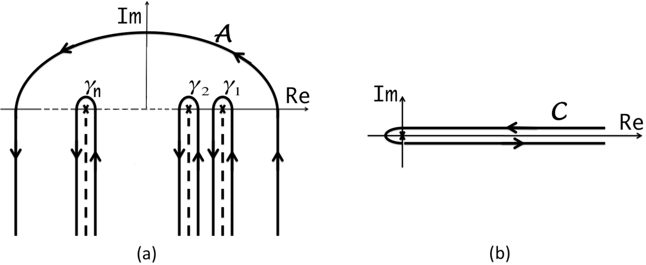
Figure 7: (a) The integration contour ${\bm{A}}$ inclosing all branch cuts (dashed lines) from a large distance. (b) Each integral over ${\bm{\gamma}_{n}}$ can be transformed into the integral over the contour ${\bm{C}}$ by a change of variables.

We introduce the anzatz

$$a_{n}(\tau)=\int_{{\bm{A}}}dse^{-is\tau}\alpha_{n}(s),\quad v(\tau)=\int_{{\bm{A}}}dse^{-is\tau}V(s),$$ (120)

where ${\bm{A}}$ is a contour such that the integrand vanishes at this contour limits. Substituting (120) in (119) we obtain a 1st order differential equation for $a_{n}(s)$, which is trivially solvable. Substituting the result back to (120) we find

$$v(\tau) = Q\int_{{\bm{A}}}ds\,e^{-is\tau}\prod_{n=1}^{N}(-s+\beta_{n})^{\frac{iq_{n}^{2}}{2}},$$

$$a_{m}(\tau) = -Qg_{m}\int_{{\bm{A}}}ds\,\frac{e^{-is\tau}}{-s+\beta_{m}}\prod_{n=1}^{N}\left(-s+\beta_{n}\right)^{\frac{iq_{n}^{2}}{2}},$$

where $Q$ is a normalization constant.

Consider a contour ${\bm{A}}$, shown in Fig. 7(a), that incloses branch cuts at $s=\{\beta_{n}\}$ from a large distance and goes to infinities at $s=-i\infty\pm R$, where $R$ is a large real number. In this limit, we can disregard terms $\beta_{n}$ in comparison with $s$, so that integrals in (LABEL:sol11) simplify, e.g.,

$$v(\tau)\rightarrow Q\int_{{\bm{A}}}e^{-is\tau}(-s)^{\frac{iE_{+}}{2}}\,ds.\\$$ (122)

In (122), the contour ${\bm{A}}$ can be transformed into the contour ${\bm{C}}$ in Fig. 7(b) by switching to the variable $z=iut$ and shrinking the contour to run around the branch cut of $z$. We can then use the formula

$$\Gamma(z)=-\frac{1}{2i{\rm sin}(\pi z)}\int_{\bm{C}}(-\tau)^{z-1}e^{-\tau}d\tau$$ (123)

to evaluate the integral. We find that, at $\tau\rightarrow 0_{+}$, this solution behaves as the state $|+\rangle$, i.e. it corresponds to the desired initial condition if one introduces the normalization factor

$$|Q|=\frac{1}{\sqrt{4\pi}\sqrt{1-e^{-\pi E_{+}}}}.$$ (124)

In order to find transition probabilities at $\tau\rightarrow+\infty$ limit, we continuously deform the contour ${\bm{A}}$ into the combination of contours ${\bm{\gamma}_{n}}$ that inclose the branch cuts at $s=\beta_{n}$ as shown in Fig. 7(a). In the limit $\tau\rightarrow+\infty$, only the vicinity of the branching points contribute essentially to each integral over ${\bm{\gamma}_{n}}$. Hence one can change variables $s\rightarrow u+\beta_{n}$, keeping the dependence on $s$ only for terms that are singular near the origin of the ${\bm{\gamma}_{n}}$-th cut. In all other factors, we can substitute $s$ by its value at this point. The $m$-th integral in (LABEL:sol11) over ${\bm{\gamma}_{m}}$ provides the asymptotic at $t\rightarrow+\infty$ for $a_{m}(t)$, i.e.

$$a_{m}(t)_{\rightarrow+\infty}=-Qg_{m}\prod_{n=1,\,n\neq j}^{N}(\beta_{n}-\beta_{m})^{i\frac{q_{n}^{2}}{2}}\int_{\bm{\gamma}_{0}}ds\,e^{-ist}(-s)^{-1+i\frac{q_{m}^{2}}{2}},$$ (125)

where we should assume that $(-i)=e^{-i\pi/2}$ and $-1=e^{-i\pi}$. Remaining integrals again can be evaluated with Eq. (123). Transition probabilities can be obtained by taking squares of the absolute values of transition amplitudes. In order to write them, it is convenient to introduce LZ-like probabilities:

$$p_{j}=e^{-\pi q_{j}^{2}},\quad j=1,\ldots,N.$$ (126)

The transition probabilities from the initially populated $|+\rangle$ state to all possible diabatic states are then given by

$$\noindent P_{+\rightarrow m}=\frac{\left((1-p_{m})\prod\limits_{n}^{\beta_{m}<\beta_{n}}p_{n}\right)}{1-e^{-\pi E_{+}}}.$$ (127)

One can verify that for the special case of $N=2$ and the case when $m$ is the index of the extremal level, Eq. (127) transfers into results presented in sections III.C and IV.D. We also note that Eq. (127) predicts that the transition probabilities do not depend on the slopes of the levels $\beta_{i}$ as far as the ordering of $\beta_{i}$ according to their magnitudes is preserved.

References

- (1) H. Nakamura, “Nonadiabatic Transition”, World Scientific Publishing Company, 2nd Edition (2012)
- (2) E. Majorana, Nuovo Cimento 9 (2), 43 (1932)
- (3) L. D. Landau, Physik Z. Sowjetunion 2, 46 (1932)
- (4) C. Zener, Proc. R. Soc. A 137, 696 (1932); E. C. G. Stückelberg, Helv. Phys. Acta 5, 369 (1932)
- (5) N. Rosen, and C. Zener, Phys. Rev. 40 502 (1932); J B. Delos and W. R. Thorson, Phys. Rev. A 6, 728 (1972); Phys. Rev. A 17, 1343 1356 (1978)
- (6) E. E. Nikitin, Adv. Quantum Chem. 5 135 (1970)
- (7) V. I. Osherov, and H. Nakamura, J. Chem. Phys. 105, 2770 (1996)
- (8) V. A. Yurovsky, A. Ben-Reuven, and P. S. Julienne, Phys. Rev. A 65, 043607 (2002); V Shahnazaryan, O Kyriienko, I Shelykh, Preprint arXiv/1410.1379 (2014); W. H. Zurek, U. Dorner, and P. Zoller, Phys. Rev. Lett. 95, 105701 (2005); B. Damski and W. H. Zurek Phys. Rev. A 73, 063405 (2006); B. Damski, H. T. Quan, and W. H. Zurek, Phys. Rev. A 83, 062104 (2011); V. Gurarie, Phys. Rev. A 80, 023626 (2009); B. E. Dobrescu, and V. L. Pokrovsky, Phys. Letters A 350, 154 (2006); M. Schecter, and A. Kamenev, Phys. Rev. A 85, 043623 (2012)
- (9) D. Sun and A. Abanov and V. L. Pokrovsky EPL 83, 16003 (2008); A. Altland, V. Gurarie, T. Kriecherbauer, and A. Polkovnikov, Phys. Rev. A 79, 042703 (2009); A. P. Itin, and P. Törmä, Phys. Rev. A 79, 055602 (2009)
- (10) M. N. Kiselev, K. Kikoin and M. B. Kenmoe, EPL 104, 57004 (2013); F. Forster et al Phys. Rev. Lett. 112, 116803 (2014); Sriram Ganeshan, Edwin Barnes, and S. Das Sarma, Phys. Rev. Lett. 111, 130405 (2013); Hugo Ribeiro, J. R. Petta, and G. Burkard, Phys. Rev. B 87, 235318 (2013)
- (11) K. Saito, M. Wubs, S. Kohler, Y. Kayanuma, and P. Hänggi, Phys. Rev. B 75, 214308 (2007); P. Ao and J. Rammer, Phys. Rev. B 43, 5397 (1991) ; M. H. S. Amin, D. V. Averin, and J. A. Nesteroff, Phys. Rev. A 79, 022107 (2009); V. N. Ostrovsky and M. V. Volkov, Phys. Rev. B 73, 060405 (2006); J. Keeling, A. V. Shytov, and L. S. Levitov, Phys. Rev. Lett. 101, 196404 (2008); M. Wubs, K. Saito, S. Kohler, P. Hänggi, and Y. Kayanuma, Phys. Rev. Lett. 97, 200404 (2006) .
- (12) C. M. Quintana, K. D. Petersson, L. W. McFaul, S. J. Srinivasan, A. A. Houck, J. R. Petta, Phys. Rev. Lett. 110, 173603 (2013); S. Masuda, K. Nakamura, and A. del Campo, Phys. Rev. Lett. 113, 063003 (2014); S. Deffner, C. Jarzynski, and A. del Campo, Phys. Rev. X 4, 021013 (2014); A. del Campo, M. M. Rams, and W. H. Zurek, Phys. Rev. Lett. 109, 115703 (2012)
- (13) S. Brundobler and V. Elser, J. Phys. A 26, 1211 (1993)
- (14) A. V. Shytov, Phys. Rev. A 70, 052708 (2004)
- (15) N. A. Sinitsyn, J. Phys. A 37 (44), 10691 (2004)
- (16) B. E. Dobrescu and N. A. Sinitsyn, J. Phys. B: At. Mol. Opt. Phys. 39, 1253 (2006); M. V. Volkov and V. N. Ostrovsky, J. Phys. B: At. Mol. Opt. Phys. 37, 4069 (2004); M. V. Volkov and V. N. Ostrovsky, J. Phys. B: At. Mol. Opt. Phys. 38, 907 (2005)
- (17) Yu. N. Demkov and V. I. Osherov, Zh. Exp. Teor. Fiz. 53, 1589 (1967) [Sov. Phys. JETP 26, 916 (1968)]; A. A. Rangelov, J. Piilo, and N. V. Vitanov, Phys. Rev. A 72, 053404 (2005)
- (18) N. A. Sinitsyn, Phys. Rev. B 66, 205303 (2002); J. Dziarmaga, Phys. Rev. Lett. 95, 245701 (2005); M. V. Volkov and V. N. Ostrovsky, Phys. Rev. A 75, 022105 (2007)
- (19) Y. N. Demkov and V. N. Ostrovsky, Phys. Rev. A 61, 032705 (2000); Yu. N. Demkov and V. N. Ostrovsky, J. Phys. B 28, 403 (1995); V. N. Ostrovsky and H. Nakamura, J. Phys. A 30, 6939 (1997); Y. N. Demkov and V. N. Ostrovsky, J. Phys. B 34, 2419 (2001); C. E. Carroll and F. T. Hioe, J. Phys. A 19, 1151 (1986)
- (20) N. A. Sinitsyn,, Phys. Rev. A, 87, 032701 (2013); V. L. Pokrovsky and N. A. Sinitsyn, Phys. Rev. B 65, 153105 (2002)
- (21) V. N. Ostrovsky, Phys. Rev. A 68, 012710 (2003)
- (22) N. A. Sinitsyn, Phys. Rev. Lett. 110, 150603 (2013)
- (23) J. Lin, and N. A. Sinitsyn, J. Phys. A: Math. Theor. 47 015301 (2014)
- (24) J. Lin, and N. A. Sinitsyn, J. Phys. A: Math. Theor. 47 175301 (2014)
- (25) J. S. Cabral et. al, New J. Phys. 12, 093023 (2010); F. Baumgartner, and H. Helm, Phys. Rev. Lett. 104, 103002 (2010); J. M. Menendez, I. Martin, and A. M. Velasco, J. Chem. Phys. 119, 12926 (2003); V. A. Nascimento, L. L. Caliri, A. Schwettmann, J. P. Shaffer, and L. G. Marcassa, Phys. Rev. Lett. 102, 213201 (2009); F. Robicheaux, C. Wesdorp, and L. D. Noordam, Phys. Rev. A 62, 043404 (2000); Yong-Lin He, J. Phys. B: At. Mol. Opt. Phys. 45 015001 (2012)
- (26) R. S. Tantawi, A. S. Sabbah, J. H. Macek, and S. Yu. Ovchinnikov Phys. Rev. A 62, 042710 (2000); J. S. Cohen, L. A. Collins, and N. F. Lane, Phys. Rev. A 17, 1343 (1978); T. R. Dinterman and J. B. Delos, Phys. Rev. A 15, 463 474 (1977)
- (27) V. P. Gurarii and V. I. Matsaev, Teoret. Mat. Fiz. 100 (1994), no. 2, 173 182; English transl., Theoret. and Math. Phys. 100 (1994), no. 2, 928 936 (1995)